the Creative Commons Attribution 4.0 License.
the Creative Commons Attribution 4.0 License.
 | 11 Apr 2022
Drought impact links to meteorological drought indicators and predictability in Spain
Herminia Torelló-Sentelles
Christian L. E. Franzke
Drought affects many regions worldwide, and future climate projections imply that drought severity and frequency will increase. Hence, the impacts of drought on the environment and society will also increase considerably. Monitoring and early warning systems for drought rely on several indicators; however, assessments of how these indicators are linked to impacts are still lacking. Here, we explore the links between different drought indicators and drought impacts within six sub-regions in Spain. We used impact data from the European Drought Impact Report Inventory database and provide a new case study to evaluate these links. We provide evidence that a region with a small sample size of impact data can still provide useful insights regarding indicator–impact links. As meteorological drought indicators, we use the Standardised Precipitation Index and the Standardised Precipitation Evapotranspiration Index; as agricultural and hydrological drought indicators, we use a Standardised Soil Water Content Index and a Standardised Streamflow Index and a Standardised Reservoir Storage Index. We also explore the links between drought impacts and teleconnection patterns and surface temperature by conducting a correlation analysis, and then we test the predictability of drought impacts using a random forest model. Our results show that meteorological indices are best linked to impact occurrences overall and at long timescales between 15 and 33 months. However, we also find robust links for agricultural and hydrological drought indices, depending on the sub-region. The Arctic Oscillation, Western Mediterranean Oscillation, and the North Atlantic Oscillation at long accumulation periods (15 to 48 months) are top predictors of impacts in the northwestern and northeastern regions, the community of Madrid, and the southern regions of Spain, respectively. We also find links between temperature and drought impacts. The random forest model produces skilful models for most sub-regions. When assessed using a cross-validation analysis, the models in all regions show precision, recall, or R2 values higher than 0.97, 0.62, and 0.68, respectively. Thus, our random forest models are skilful in predicting drought impacts and could potentially be used as part of an early warning system.
- Article
(3781 KB) - Full-text XML
-
Supplement
(184 KB) - BibTeX
- EndNote


Drought, as defined by Wilhite and Glantz (1985), “is a condition relative to some long-term average condition of balance between rainfall and evapotranspiration in a particular area, a condition often perceived as 'normal”'. The prediction of drought onset or end is a complex task. Drought severity is also difficult to measure or quantify. This is because drought depends on several factors, for instance, the duration, intensity, and the geographical extent of the event. Additional factors specific to each region also play a large role, such as the water demand with respect to water supply. All of these characteristics make drought difficult to identify and quantify. Drought has far-reaching impacts on society and the environment that may last for long time periods (Wilhite and Glantz, 1985).
There is not a common and straightforward definition of drought; however, all types of drought originate from a lack of precipitation. Many different definitions of drought have been developed by different disciplines. There are four main types of disciplinary definitions, i.e. meteorological, agricultural, hydrological, and socioeconomic. Meteorological drought often uses precipitation as its atmospheric parameter. Agricultural drought considers links between meteorological drought and its impacts on agriculture. Hydrological drought accounts for the repercussions of dry periods on surface and subsurface hydrology, for instance, on streamflow, groundwater, and reservoirs. Finally, socioeconomic drought considers the effects that drought has on the supply and demand of economic goods (Wilhite and Glantz, 1985).
There is already evidence that climate change, as a result of anthropogenic actions, has increased the risk of meteorological drought in southern Europe (Gudmundsson and Seneviratne, 2016). Similarly, warmer temperatures have increased atmospheric evaporative demand, which has in turn increased drought severity over the past 50 years (Vicente-Serrano et al., 2014b). Climate change projections point towards a reduction in the water resources in Spain. Hydraulic infrastructures have been designed with safety margins; however, these may be surpassed due to the effects of climate change. Increased evapotranspiration, as a result of increased temperatures, together with a possible increase in the length of the irrigation period, might increase the water demand for irrigation and for agricultural use, which currently accounts for more than 70 % of total water demand. In addition, the energy sector is also dependent on the availability of water, which also makes it vulnerable to increased drought risk (Ministerio para la Transición Ecológica y el Reto Demográfico, 2020). Vulnerability to water scarcity and drought is also likely to increase due to challenges such as a growing population, population migration to more arid regions, urbanisation, increasing tourism, and pollution (Rossi and Cancelliere, 2013). As a result, the consequences of drought on the environment and society are becoming more important. Spain is a country that already has an intense use of water resources; hence, it is crucial to reinforce water management to provide future water security.
In order to lessen the impacts of drought on society and the environment, efficient mitigation measures are necessary. This means that effective drought monitoring and early warning systems (DEWSs) are essential. DEWSs reduce societal vulnerability to drought by maximising the lead time of early warnings to allow more time for the implementation of mitigation measures (Pozzi et al., 2013). These systems usually rely on different drought indicators that represent different parts of the water cycle. Drought indicators describe drought conditions, and examples of commonly used variables are precipitation, temperature, streamflow, groundwater and reservoir levels, soil moisture, and snowpack (Svoboda et al., 2016). DEWSs use a large variety of drought indicators, and the most commonly used one is the Standardised Precipitation Index (SPI; McKee et al., 1993). DEWSs usually use indicators based on variables that can be measured with ease and that are readily obtainable in time (Bachmair et al., 2016a). However, Bachmair et al. (2016a) revealed that although there has been increasing efforts on the research and practice of drought indicators, DEWSs are still not well linked with assessments on how drought impacts the environment and society. This is because links between drought indicators and impacts have not been sufficiently studied. This means that impact data are not being used to determine whether indicators are linked to the impacts of drought. The authors call for drought to be framed as a coupled dynamical system of the environment and society to fully understand drought impacts.
Drought-related impacts are complex to study and document because many sectors depend on water availability to produce goods and provide services. Bachmair et al. (2016a) also revealed that there are very few systematic approaches for the collection of impact data, except for agricultural drought. A good example of efforts to improve such documentation exists in Europe, where a drought impact inventory has been created, i.e. the European Drought Impact Report Inventory (EDII; Stahl et al., 2016). This database collects reported drought impacts for different European countries. Impacts are classified into major impact categories (e.g. agriculture and livestock farming, wildfires, public water supply, and forestry), and each category has several sub-types. Also, each drought impact event has, at the very least, information on the source of information, location, duration, and impact category and has a description.
Here, we investigate the links between different drought indicators and reported impacts from the EDII database for Spain. The time period studied is from August 1975 to May 2013. We aim to assess two meteorological indicators, the SPI and the Standardised Precipitation Evapotranspiration Index (SPEI; Vicente-Serrano et al., 2010), two hydrological indicators, streamflow and reservoir storage levels, and an agricultural indicator, soil water content. The main motivation for this study is to provide a new case study for the evaluation of these links and to test the usefulness of impact data in this region. Impact data from the EDII has already shown links with drought indicators in similar studies (Bachmair et al., 2015, 2016b; Stagge et al., 2015).
The first objective of the study is to investigate how strong and robust the link between drought indicators and drought impacts is. We conduct a correlation analysis, and to further examine these indicator–impact links, we then use machine learning (a random forest model) to model and predict drought impact occurrences. Another goal of this analysis is to test the potential of such a method, with the available data, to predict future impacts. We aim to determine whether drought impacts can be skilfully predicted in this region.
To our knowledge, links between teleconnection patterns or temperature and drought impacts using the EDII database have not been studied before. We therefore investigate five teleconnection patterns (Feldstein and Franzke, 2017), the El Niño–Southern Oscillation (ENSO), the North Atlantic Oscillation (NAO), the East Atlantic (EA) pattern, the Western Mediterranean Oscillation (WeMO), and the Arctic Oscillation (AO), as well as a surface temperature index, as possible predictors of drought impact occurrences. We aim to investigate whether these climate indices show links and are better predictors of impacts than the previously presented drought indicators. Our next objective is to determine what type of indicators are the best predictors of impacts in each sub-region. Last, the incompleteness of the impact reports from the EDII database challenges the quantification of impact occurrences, hence, we also investigate different ways to take incomplete reports into account. We investigate whether different impact quantification methods change the results in a significant way and, if so, how.
Our paper is structured as follows: in Sect. 2, we introduce the study area, the drought indicators, climate indices ,and vulnerability factors used and their data sets. Also, we show how we deal with incomplete impact data and the methods for the data analysis. In Sect. 3, we present the results of our correlation and random forest analyses. In Sect. 4, we provide a discussion of our results and conclude.
2.1 Study area
Spain is located in a geographical area with a high recurrence of drought events due to it being in a transition zone between polar and subtropical atmospheric circulation influences (Sivakumar et al., 2011). Its precipitation and runoff patterns are highly diverse and complex, which is characteristic of the Mediterranean area. As described by Vide (1994), the characteristic climate of Spain has the following:
-
modest rainfall overall,
-
high interannual variability, with a high amount of rainfall occurring during relatively few days,
-
long dry periods,
-
an arid climate, meaning the amount of potential evapotranspiration is greater than rainfall,
-
large regional variations in seasonal rainfall patterns, and
-
anomalies that may be related to atmospheric teleconnection patterns.
Because of the chaotic patterns of precipitation, Spaniards have been attempting to increase water availability for at least the last 2000 years (del Moral and Saurí, 1999). Water scarcity and frequent droughts are recurrent problems that Spain suffers, and this is mainly because the spatial and temporal distribution of its water resources is irregular. This also occurs because water demands are highest in the more water scarce areas and during the seasons when precipitation is the lowest and evapotranspiration the highest. Climate change will most likely exacerbate the existing problems with water resources (Estrela and Vargas, 2012; Ministerio de Medio Ambiente, 2005).
Droughts cause extensive impacts in Spain; for instance, during a very intense drought event in 1991–1995, the water supply was restricted for more than 25 % of the total population (12 million people). In the most affected regions, evacuation plans were enacted. Agricultural production was also severely affected (del Moral and Hernandez-Mora, 2015). The major drought event in 2004–2005 led to social unrest and created disputes over future water infrastructure (Iglesias et al., 2009). Drought periods can impose significant costs on farmers and affect crop productivity (e.g. Iglesias et al., 2003; Austin et al., 1998; Páscoa et al., 2017; Peña-Gallardo et al., 2019). Moreover, vegetation activity has been shown to be linked to the interannual variability in drought (Vicente-Serrano et al., 2019), and drought has been related to burned areas from wildfires (Russo et al., 2017). Drought events have also shown links with daily mortality across Spain (Salvador et al., 2020). Overall, the economic damages of drought are severe. According to the international Emergency Events Database (EM-DAT; Guha-Sapir et al., 2016), Spain ranked fourth worldwide and first in Europe for total economic damages resulting from drought events from 1990 to 2018 (USD 7.7 billion).
We chose to perform this study in the specific region of Spain because this region is severely impacted by droughts; hence, a better understanding of indicator–impact links here is urgently needed. Such links have been already been successfully investigated in five other European regions (Bachmair et al., 2015, 2016b; Stagge et al., 2015). We focus on characterising these links in six sub-regions within Spain because studying a small region means that indicator–impact links can be better detected and quantified (Blauhut et al., 2016).
We also chose this region to investigate indicator–impact links in a region that has a very dense network of reservoirs and to investigate the timescales at which drought conditions lead to drought impacts. As described by González-Hidalgo et al. (2018), Spain has a high density of hydraulic reservoirs. Spain has, after China, the second largest number of dams in the world. This is because Spain's climate is characterised by dry summers and high interannual variability. Such a dense network increases Spain's resilience to short-term droughts by guaranteeing water supply during these events. However, at longer timescales, drought conditions still produce severe drought impacts to water supply; conditions that last more than 2 or 3 years have been shown to reach the limits of the capacity of these infrastructures (González-Hidalgo et al., 2018).
2.2 Drought indicators and data sets
As drought indicators, we considered the SPI, the SPEI, and a streamflow index because these are commonly used in DEWSs (Bachmair et al., 2016a). The SPI and especially SPEI have also shown higher correlations than other drought indices with crop yields in Spain (Peña-Gallardo et al., 2019). Furthermore, we included an additional hydrological indicator (using reservoir storage data) and an agricultural drought index (using soil water content data) to compare their performance against the other types. Soil moisture has been found to be an important factor when studying drought impacts on the productivity of some agricultural crops in Spain (Sainz de la Maza and Del Jesús, 2020). Furthermore, the multi-scalar nature of all these drought indicators is useful when assessing the timescales of drought impacts. We also explored the use of several teleconnection patterns (Feldstein and Franzke, 2017) as predictors of drought impacts.
The SPI is a commonly used drought index that is simple to compute. It can be used to compare droughts in different regions, and it can be temporally aggregated over different timescales (Guttman, 1999). It calculates “the precipitation deviation for a normally distributed probability density with a mean of zero and standard deviation of unity” (McKee et al., 1993). It is computed by fitting precipitation data to a distribution and then transforming it to a normal distribution (McKee et al., 1993). In this study, we calculated the SPI using the SPEI R package (Vicente-Serrano et al., 2010; Beguería et al., 2014). We used a gamma probability distribution to model the observed precipitation values.
The SPEI is a similar index to the SPI, but instead of being computed with precipitation values only, it is based on climatic water balance. The climatic water balance is a monthly difference between precipitation and potential evapotranspiration (PET) at different timescales. This provides a measure of the accumulated water surplus or deficit. We used the approach of Vicente-Serrano et al. (2014b) to calculate the PET; this is a simple approach that only requires data for monthly mean temperature and uses the Thornthwaite equation (Thornthwaite, 1948). To obtain the final index, the same procedure as for the SPI was followed; however, a log-logistic probability distribution was used to model the precipitation–PET values. We also calculated the SPEI with the SPEI R package. This index accounts for the effects of temperature variability on drought. The advantages of this index, especially under global warming conditions, are that it identifies increased drought severity when the water demand is higher as a result of increased evapotranspiration. In addition, its multi-scalar nature allows its use for drought analysis and monitoring (Vicente-Serrano et al., 2010).
Volumetric soil water is the volume of water (m3) in a soil layer (m3). We used this variable to create an agricultural drought indicator, a Standardised Soil Water Content Index (SSWI), using the Standardised Drought Analysis Toolbox (Hao and AghaKouchak, 2014; Farahmand and AghaKouchak, 2015a). This toolbox provides a generalised framework for deriving nonparametric univariate indices that can be interpreted similarly to the rest of the indices used in this study. This index was calculated at four different soil depths (defined by the data set used), hereafter referred to as SSWI1, SSWI2, SSWI3, and SSWI4. To create a Standardised Streamflow Index (SSFI) and a Standardised Reservoir Storage Index (SRSI), we standardised streamflow and reservoir values using the same methodology as for SPI. We also computed a Standardised Temperature Index (STI) using the same methodology, with surface temperature data only.
All of the indices were aggregated over different timescales. The aggregation of the SPI, SPEI, SSFI, and SRSI was done prior to fitting them to a distribution and transforming to the normal distribution. This means that the data for the current month and past X months was used to compute the value for a given month. The aggregation period is hereafter labelled with the suffix “-X” (e.g. SPI-X). Similarly, for the SSWI, the aggregation was done prior to computing the empirical distribution.
We chose teleconnection patterns that could potentially be relevant as drought predictors. The chosen climate indices have shown correlations with precipitation in Spain (e.g. Rodó et al., 1997; Martinez‐Artigas et al., 2021; Ríos-Cornejo et al., 2015), and the NAO, EA, AO, and WeMO have also shown links with the drought index, SPEI (Manzano et al., 2019). The effects of the NAO on droughts using the SPI and/or SPEI at the European scale are also well studied (Vicente-Serrano et al., 2011; Kingston et al., 2015). Furthermore, empirical links between drought impacts and ENSO and NAO in Spain have already been established. For instance, Gimeno et al. (2002) looked at the influence of ENSO and the NAO on the most important Spanish crops. They detected significant effects on the yield for most of these crops. They found low yields during La Niña years and higher yields during positive NAO phases. All of the climate indices were aggregated by computing a moving average over X months.
We used the Iberia01 daily precipitation and temperature observational gridded data set to calculate the SPI and SPEI (http://hdl.handle.net/10261/183071, last access: 9 March 2020; Gutiérrez et al., 2019; Herrera et al., 2019). This is a high-resolution data set produced using a dense network of stations over the Iberian Peninsula, with 3481 and 276 stations for precipitation and temperature, respectively. Gridded values are provided at a spatial resolution of 0.1∘, and they cover the entire time period studied here. This data set has been shown to produce more realistic patterns in the case of precipitation than other frequently used data sets. We used data from individual streamflow and reservoir-level monitoring stations from Ministerio para la Transición Ecológica y el Reto Demográfico (2022) to calculate the SSFI and SRSI. There were a total of 1447 and 367 streamflow and reservoir storage monitoring stations, respectively; however, after removing stations with more than 20 % missing data, data from 786 and 322 stations remained. We obtained volumetric soil water content data from the ERA5-Land data set (Muñoz Sabater, 2019). This is a reanalysis data set that provides estimates for land variables. It has a horizontal spatial resolution of and has a vertical resolution that consists of four levels of the surface at 0–7 cm (layer 1), 7–28 cm (layer 2), 28–100 cm (layer 3), and 100–289 cm (layer 4). We obtained data for the NAO, EA, AO, and ENSO from the NOAA Climate Prediction Center (https://psl.noaa.gov/data/climateindices/list/, last access: 2 August 2021 and https://www.cpc.ncep.noaa.gov/data/teledoc/ea.shtml, last access: 2 August 2021) and data for the WeMO (Martin-Vide and Lopez-Bustins, 2006) from http://www.ub.edu/gc/wemo/ (last access: 2 August 2021). We used data from these data sets for the period 1975–2013, except for volumetric soil water content data, where we used data from 1981–2013, since data were only available starting from 1981. We also aggregated all the indices over a range of timescales. These ranges differed depending on up to which timescales the indicator–impact correlation strengths were greatest. These were 1–33 months for the SPI, SPEI, and SRSI and 1–48 months for the SSWI, STI, and teleconnection patterns.
The nomenclature of territorial units for statistics (Nomenclature des Unités territoriales statistiques – NUTS) classification divides economic territories of the European Union (Eurostat, 2020). NUTS-1 regions represent major socioeconomic regions, and these were the sub-regions we considered in this study. These were the northwest (NW), northeast (NE), community of Madrid (MA), centre (CE), east (E), and south (S). The Canary Islands were excluded due to a lack of impact data in this region. We aggregated all of the indicators studied over each NUTS-1 region and produced a mean monthly time series for each sub-region using the R package panas (De Felice, 2020).
2.3 Drought vulnerability and data sets
To understand how a region is impacted by drought, drought risk needs to be considered as a function of the hazard, vulnerability, and exposure to drought events. “Vulnerability refers to the propensity of exposed elements such as human beings, their livelihoods, and assets to suffer adverse effects when impacted by hazard events” and “exposure refers to the inventory of elements in an area in which hazard events may occur” (Cardona et al., 2012). Exposure varies spatially, and vulnerability depends on social and economic factors of a region, which can greatly change over time (Wilhite, 2000).
To explain the drought impacts beyond the hazard, we also investigated whether adding vulnerability factors as drought impact predictors would increase the predictability of drought impact models. We used data for public water supply, unemployment rate, population density, gross domestic product (GDP) per capita, and gross value added (GVA) by industry (except construction), by agriculture, forestry, and fishing, and by the Statistical Classification of Economic Activities in the European Community (NACE) activities. We also used land cover data from the CORINE Land Cover data set and calculated the percentage of each land cover class per NUTS-1 region. A monthly time series was created for each vulnerability factor from yearly or 6-year data by linearly interpolating the data points. We obtained the data from the Instituto Nacional de Estadística (https://www.ine.es, last access: 6 September 2021), Eurostat (https://ec.europa.eu/eurostat/, last access: 10 November 2021), and the CORINE Land Cover data set (https://land.copernicus.eu/pan-european/corine-land-cover, last access: 12 November 2021). Most of these factors have been reviewed and tested as drought vulnerability factors by Blauhut et al. (2016).
2.4 Drought impact data
We retrieved drought impact information from the EDII. This database had 388 impact report entries for Spain, which covered the time period from August 1975 to May 2013. Each reported impact has three spatial references which correspond to the three levels of the NUTS regions. We aggregated the impact information by NUTS-1 region and did not differentiate impact types from one another; hence, we treated all impacts as equal and of a general type. The impact categories considered in the EDII were as follows:
-
Agriculture and livestock farming
-
Forestry
-
Freshwater aquaculture and fisheries
-
Energy and industry
-
Waterborne transportation
-
Tourism and recreation
-
Public water supply
-
Water quality
-
Freshwater ecosystem: habitats, plants and wildlife
-
Terrestrial ecosystem: habitats, plants and wildlife
-
Soil system
-
Wildfires
-
Air quality
-
Human health and public safety
-
Conflicts.
In order to evaluate links between indicators and impacts, we mainly followed the methodology by Bachmair et al. (2015, 2016b), who assessed links between hydro-meteorological indicators and impacts for Germany and the UK. We first explored correlations between indicators and impacts, and we then used a random forest model to evaluate the predictive potential and predictor importance of the different indicators. Before conducting the analysis, we first converted impact reports into a monthly time series of the number of drought impact occurrences for each sub-region. To do this, we imposed criteria to convert a single drought impact report (an entry from the EDII) into a drought impact occurrence, which will be referred to as DIO. We converted impact reports into a monthly time series by creating a DIO for every month in between the start and end date. However, a large proportion of the reports were incomplete. The data had the following five main problems:
-
The specific sub-region affected was not indicated.
-
The start and the end year were indicated, but there was no indication of the start and end month.
-
The start year was indicated, but there was no indication of the end year or start and end month.
-
The start month was indicated, but there was no indication of the end month and year.
-
The start month and the end year were indicated, but there was no indication of the end month.
In total, 24 % of the reports had problem 1, 33 % had problem 2, 37 % had problem 3, 9 % had problem 4, and 3 % had problem 5. Therefore, to overcome and estimate the uncertainty in our analysis as a result of the incompleteness of the data, we developed different counting methods. This meant that we tested the effects of including or excluding reports with these problems. The counting methods (CM) are described in Table 1.
We visually examined impact reports, specifically their durations and descriptions, to make sure that their quantification to impact occurrences was sensible regarding the nature of each impact. For instance, we made sure that impacts that usually do not last more than 1 month by nature were reported in such a way. Some of these impact types were wildfires, air quality, human health, and public safety. Quantifying more long-lasting impacts, such as impacts on agriculture and livestock and freshwater and terrestrial ecosystems, was more challenging, since determining their exact start and end dates is not possible. However, we still used the start and end dates of these reports, since we believe that these represent the period during which sectors were most affected by drought impacts. For example, for a report that stated that “livestock farming economic losses are estimated to be EUR 39.372 million for the period 1 November 2004–30 April 2005” (Stahl et al., 2016), we assumed that the occurrence of these economic losses corresponds to the period during which the sector was most affected by drought impacts.
Table 1How drought impact occurrences (DIOs) are counted in each counting method.
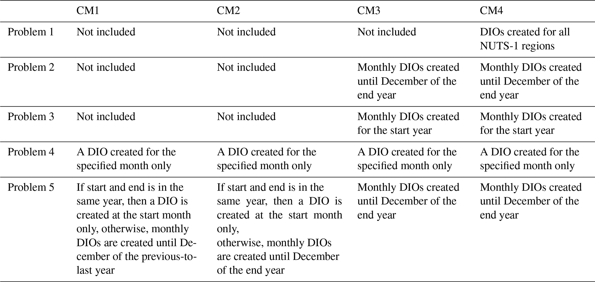
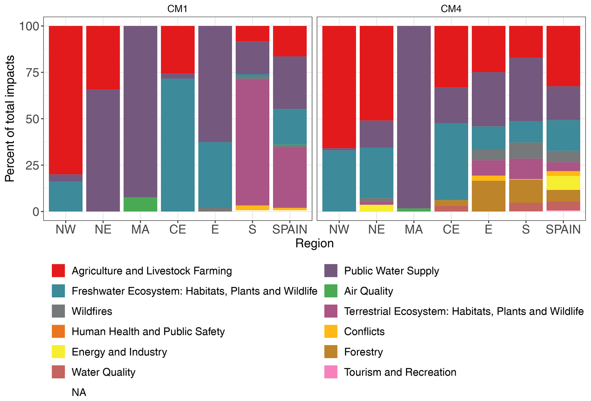
Figure 1Distribution of impact types for Spain and the sub-regions studied. Results for the most and least censoring counting methods (CM1 and CM4) are shown.
Figure 1 shows the distribution of impacts types for each NUTS-1 region and for the whole of Spain using the most and least censoring counting methods. It shows that most of the impacts recorded in the EDII for Spain were on agriculture and livestock farming, public water supply, and freshwater ecosystems. Also, depending on the censoring criteria, the distribution of impact types varied slightly. For instance, the most censoring counting methods showed a larger proportion of impacts on terrestrial ecosystems in the S region and for the whole of Spain. The least censoring methods also had a larger variety of impact types.
Aggregating all impact types to a single category is not an optimal choice, since focusing on sector-specific drought impact occurrences separately would produce more informative results. However, each sub-region contains three or fewer types of impact categories, except the S region which contains eight (Fig. 1, CM1). This meant that there were not enough data points to investigate categories separately.
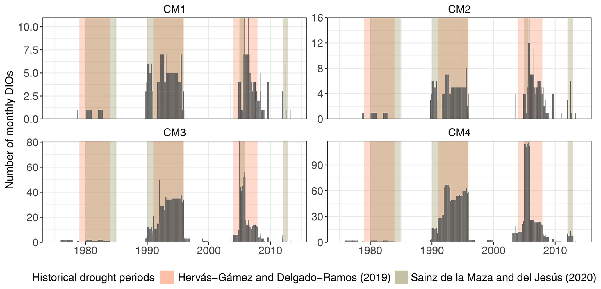
Figure 2Total monthly DIOs in Spain (bars) from 1975 to 2013, using different counting methods (CM1–CM4). Important historical drought periods identified in other studies are highlighted.

Figure 3Monthly DIOs (bars) in each sub-region from 1975 to 2013, using the most censoring counting methods (CM1 and CM2). Important historical drought periods identified in other studies are highlighted.
Figure 2 shows the time series of total DIOs for Spain and also shows identified precipitation deficit episodes in which Spain suffered major impacts due to severe drought and water scarcity events (Hervás-Gámez and Delgado-Ramos, 2019). Historical drought periods identified by Sainz de la Maza and Del Jesús (2020), determined from economic impacts of past droughts, are also shown. The latter authors identified these by using data from the EM-DAT and from another study (Ollero Lara et al., 2018) that used insurance data by the Entidad Estatal de Seguros Agrarios (National Agricultural Insurance Agency). Figure 2 shows that most of the DIOs occurred during the identified historical drought periods by the authors mentioned. A slight disagreement occurs in 2008 until late 2009, where DIOs continue to occur even though the reported drought episodes end in 2007. Moreover, Fig. 3 shows the time series of DIOs for all sub-regions (see Fig. S1 in the Supplement for DIOs when using the two least censoring counting methods). We observe that, during each drought episode, DIOs do not always occur in all sub-regions, and that the amounts and patterns of DIOs do change between counting methods, depending on the harshness of the censoring criteria.
2.5 Correlation analysis
Table 2Information on DIOs for the different sub-regions and the length of the time series for analysis for the most censoring counting method (CM1).
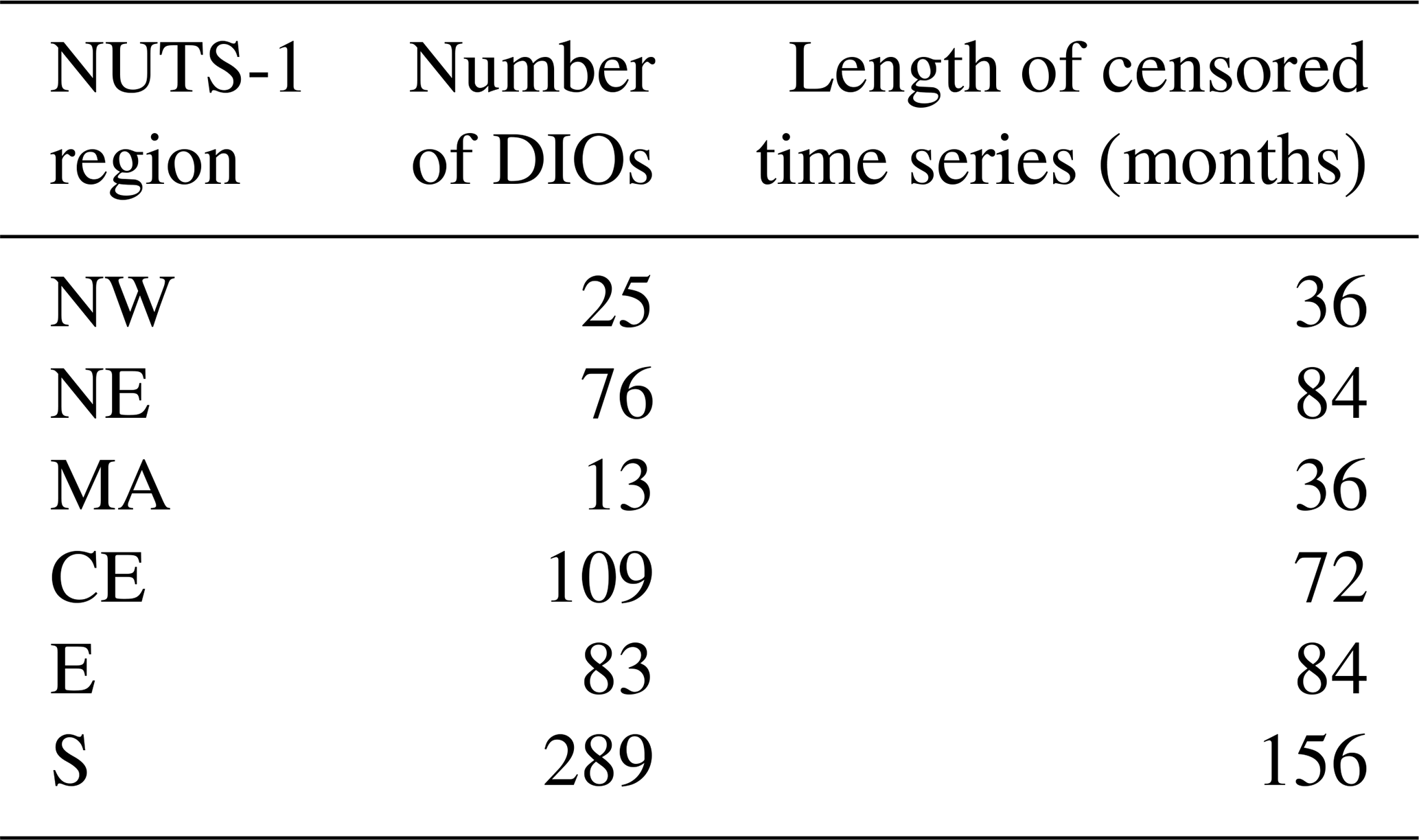
For each NUTS-1 region, we selected a subset of years from August 1975 to December 2013 for the analysis. This selection excluded years where no impact occurrences were reported. We then included each month of each selected year in a censored time series. We did this to exclude years in which regions may have experienced drought impacts but which may not have been recorded in the EDII. The lengths of the censored time series are shown in Table 2. To determine the relationship between drought indicators and drought impacts, we first conducted a cross-correlation analysis. We calculated the Spearman rank correlation coefficients (Spearman, 1961) and the significance levels for the time series of different indicator versus the time series of DIOs for each NUTS-1 region. For each indicator, we spatially aggregated the indicators over each NUTS-1 region using their mean.
2.6 Random forest analysis
A random forest (Breiman, 2001) is a machine learning approach that uses ensemble trees. This approach has already been used to link drought indicators to impacts (Bachmair et al., 2016b, 2017) and even to forecast drought impacts (Sutanto et al., 2019). A random forest is a tree-based ensemble; each tree depends on a random sample of predictor variables and a random response variable. The model then creates a prediction function to predict the response variable by constructing ensembles of trees. The predictions over all trees are combined by being averaged (in regression models) or by selecting the class that is more frequently predicted (in classification models) (Cutler et al., 2012). Random forest models are appealing because the predictor and response variables can either be continuous or categorical variables. It is a fast model to run computationally, and very few tuning parameters are required. Apart from training and making predictions, they can also provide variable importance measures. Random forest models also require minimal human supervision (Cutler et al., 2012).
In this study, we used random forest models to model drought impacts, using the R package randomForest (Liaw and Wiener, 2002). We trained two models for each NUTS-1 region, i.e. a regression and a classification model. For the regression models, we used a time series of normalised DIOs as the response variable and the monthly time series of drought indicators as predictors. The number of DIOs was normalised by dividing them by the total number of DIOs for each region. This allowed for a fair comparison of the model errors between regions and counting methods. For the classification models, we used a binary time series of impacts, which was constructed by categorising the response variable by setting DIO =0 to no impact and DIO >0 to impact. Including this binary signal time series also considered the fact that the reporting of drought impacts might have changed over the years due to improvements in reporting and data collection. For instance, it excluded a potential bias in DIOs (upward trend observable in Fig. 2).
Unlike the correlation analysis, the DIO time series were not censored in this analysis. As predictors, we included all the indicators mentioned earlier aggregated over the different timescales. We identified the best predictors for each region using the variable importance feature. The algorithm estimates the variable importance by examining by how much the prediction error increases when that variable is excluded from the model (Liaw and Wiener, 2002).
The main input parameters in a random forest model are the number of trees, ntree, and the number of variables randomly sampled at each split, mtry. As Breiman (2001) mentions, for a large number of trees, and as the number of trees increases, the generalisation error converges to its limiting value. We set ntree equal to 1000. In order to select the optimal mtry parameter for each model, we used the R package caret (Kuhn, 2008) for tuning the models. We also used this package to perform a cross-validation analysis.
To assess the predictive potential of the random forest models, we first conducted a 10-fold cross-validation analysis using all of the available data (June 1983 to December 2013) repeated five times. We used the root mean squared error (RMSE) and R2 performance metrics to evaluate the regression models. To assess the classification models, we used receiver operating characteristic (ROC) curves and area under the ROC curve (AUC). The AUC assesses the quality of a forecast of binary outcomes. These measures consider the proportion of impact occurrences correctly predicted and the proportion of (wrongly) predicted occurrences when there were none (Mason and Graham, 2002). Because we found large imbalances in the event classes (a large number of no impact events with respect to impact events), we also used precision, recall, and F score metrics to assess the models. These metrics better assess model performance in this case (Davis and Goadrich, 2006). Precision is the number of impact occurrences correctly predicted as a proportion of the total impact occurrence predictions made, and recall is the proportion of impact occurrences correctly predicted (Davis and Goadrich, 2006). The F score is a combination of precision and recall as their harmonic mean (Hripcsak and Rothschild, 2005).
In order to further evaluate the performance of the models, we randomly partitioned the data into a training and testing part, with a 75:25 split. We tuned and trained the models (using a 10-fold repeated cross-validation) to then predict the testing set. In this analysis, we also compared the two types of models, i.e. classification and regression. We did this by converting the outputs of the regression model into binary classes. The threshold to classify the outputs was set to 0.5, 1, 1.25, and 1.5; outputs below each threshold were classified as no impact, and outputs above each threshold as impact. These thresholds were then normalised by dividing by the total number of impact occurrences in each region.
3.1 Correlation analysis
Figure 4 shows significant correlations for the indicators in most regions. This indicates that there are clear links between drought indicators and impact occurrences for most regions. Overall, the results from this analysis show that drought impact occurrences are negatively correlated to the drought indicators studied, and when not, the correlation values were usually weak or not significant. Drought indices are negative during a period of drought; this means that when the drought indicator severity increases, then the impact occurrences tend to increase and vice versa. The NE and CE regions show the lowest correlations for all indicators; this indicates that these regions show the weakest links with impact occurrences. In this analysis, neither the total number of impact occurrences nor the length of the censored time series (see Table 2) seemed to be related to correlation strength. For instance, these two regions were the regions with the fourth- and second-highest number of impact occurrences, respectively, but they showed the weakest links. As mentioned earlier, the drought risk is also affected by a region's exposure to drought. This could explain why we find the weakest hazard–impact correlations in two of the least populated regions (NE and CE), since the impacts are reported by a region only when it has been exposed to the hazard and has been vulnerable to it.
The SPI and SPEI showed a similar performance to one another, with the exception of the S region, where the SPI showed a larger number of significant and strong correlations. Aggregations over timescales of 18–21 months showed the highest correlations for both indicators. Moreover, the agricultural indicator, SSWI3 showed the greatest number of significant and strong correlations out of the remaining soil layers. SSWI4 outperformed SPI and SPEI in the S region at a timescale of 18 months; however, its overall performance was lower, especially in the CE and NE regions. The hydrological indicator, SSFI, showed strong and significant correlations in most regions but underperformed in the CE region, when compared to the SPI and SPEI. It also showed very similar patterns to the SSWI but with a slightly better performance in the NE region. SRSI showed strong significant correlations in the MA and S regions and had slightly lower strength in the NE and E regions.

Figure 4Correlation coefficients (ρ) between time series of drought indicators and impact occurrences for each sub-region, using one of the most censoring counting methods (CM1). Asterisks indicate the significance (p<0.05).
Table 3Correlation coefficients (ρ) between drought indicators and climate indices, and impact occurrences for the two most censoring counting methods (CM1 and CM2). The indices are ordered by decreasing correlation strength and the timescale at which the indices are aggregated (sc) is shown.
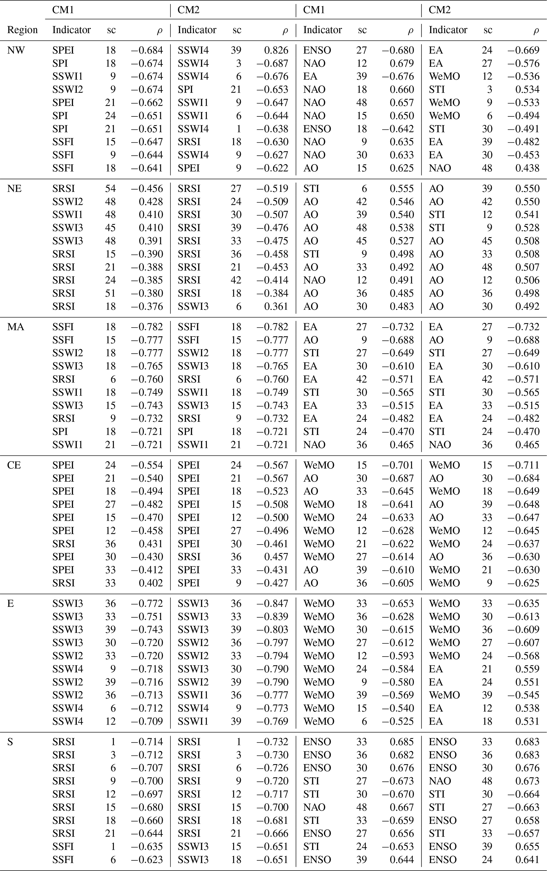
When comparing the correlation patterns across different counting methods, we found that, overall, the two most censoring counting methods had the highest average correlation coefficients and smallest average p values over all regions, indicators, and aggregation timescales. Correlation patterns remained very similar for the two most censoring counting methods, except for the SRSI, in that one method showed significant correlations in one region (NW) and did not show this when using the other method. The two least censoring methods showed similar patterns to the two other methods in four sub-regions (MA, CE, E, and S); however, most significant correlations disappeared in the remaining two regions (NW and NE; see Fig. S2). We found that, generally, the less censoring the method, the lower the correlation strengths. These results indicate that counting methods do, to some extent, affect correlation patterns and strengths between indicators and impact occurrences. The results obtained here indicate that it is important to investigate different counting methods when working with incomplete impact data. In the following, we will use the two most censoring counting methods to determine the links between indicators and impacts, since the results were most consistent when using these two counting methods. The predictors that showed the highest correlation strengths using these counting methods are displayed in Table 3. A comparison of the correlations of CM1 and CM2 in Table 3 shows that correlations are usually very close in value. The two counting methods also show similar results, since the same indicators are usually present in both columns, especially for the drought indices.
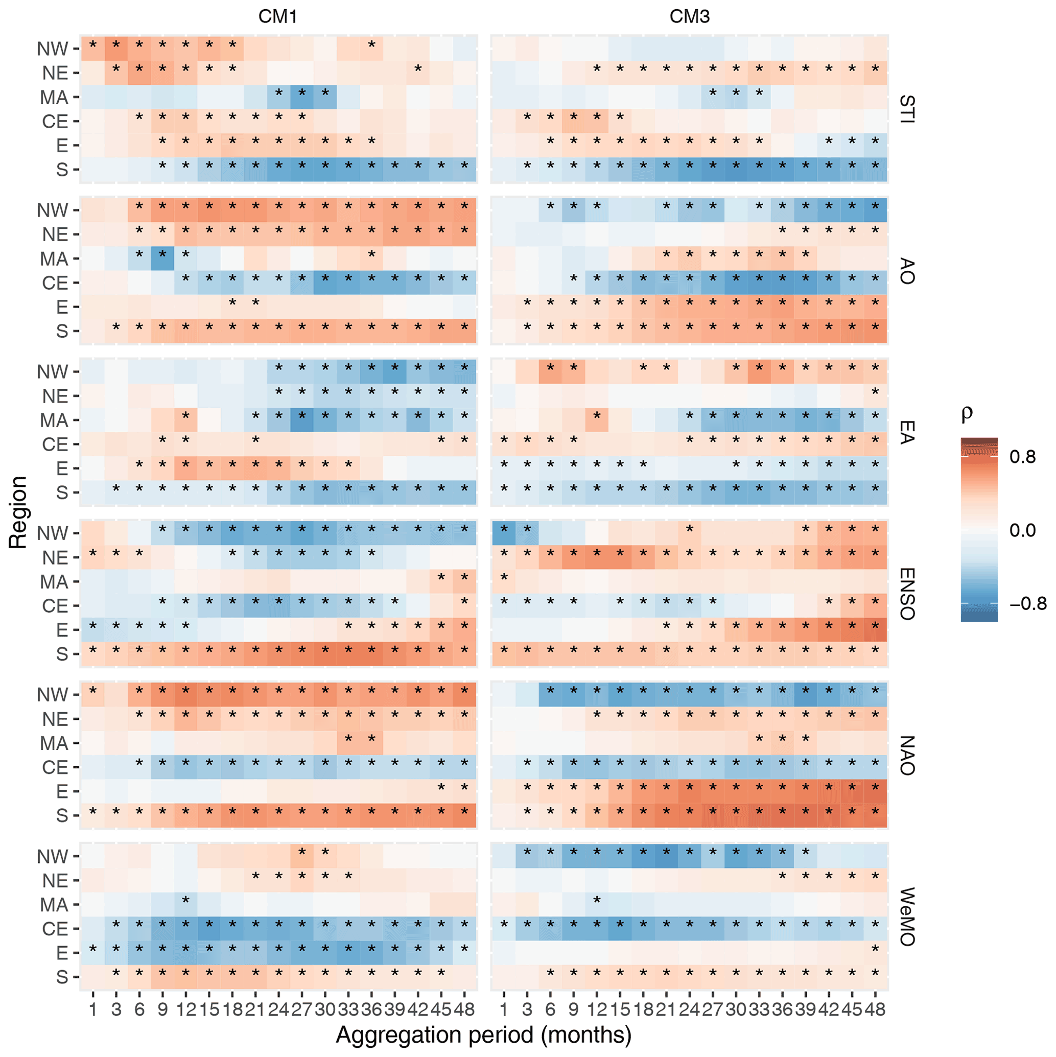
Figure 5Correlation coefficients (ρ) between time series of climate indices and impact occurrences for each sub-region using one of the most (CM1) and the third most (CM3) censoring counting methods. Asterisks indicate the significance (p<0.05).
Overall, the teleconnection patterns and STI (Fig. 5) showed strong and significant correlations with impact occurrences for many sub-regions and timescale aggregations when using the two most censoring counting methods. However, the main difference when compared to the correlation patterns with the drought indicators in Figs. 4 and S2, is that the correlation directions varied across the different sub-regions and counting methods here. This behaviour can be due to there being a negative linear relationship between the two variables or due to a lag between indices and impact occurrences. For example, although STI correlated negatively with impacts in the MA region, when we compared both time series (not shown) we saw that impact occurrences appeared during an abnormally hot period but appeared at a time when there was a short period of decreasing temperatures. This suggests that there is lag between elevated temperatures and impact occurrences in this region. Excluding the MA and S regions, the STI and impact occurrences showed positive correlations. This suggests that there is a positive linear relationship between temperature anomalies and drought impact occurrences.
The correlation patterns using the two most censoring counting methods (Fig. 5) showed that EA at 24–39 months has the strongest correlations in the NW region, with AO at 39–48 months and STI at 6–12 months in the NE region, EA at 27–39 months, AO at 9 months and STI at 27–30 months in the MA region, WeMO at 12–24 months and AO at 30–39 months in the CE region, WeMO at 27–36 months in the E region, and ENSO at 30–36 months, STI at 27–30 months, and NAO at 48 months in the S region. These results are also displayed in Table 3. Out of all the teleconnection patterns, the NAO and AO showed very similar correlation patterns to each other, which is to be expected since both are dynamically related (Feldstein and Franzke, 2006).
The third most censoring counting method showed similar patterns to the two most censoring methods, except for two sub-regions (NW and NE) where the most significant correlation patterns disappeared or changed direction. The least censoring method overall still showed significant correlations but with decreased strength. Therefore, we again find that counting methods sometimes affected correlation patterns. We must also take into account that a correlation analysis only assesses links between two variables; however, the pathways by which these patterns affect drought conditions and the propagation to impacts are usually complex. Possible interactions between different teleconnection patterns or other atmospheric phenomena were not modelled in this analysis due to its bivariate nature.
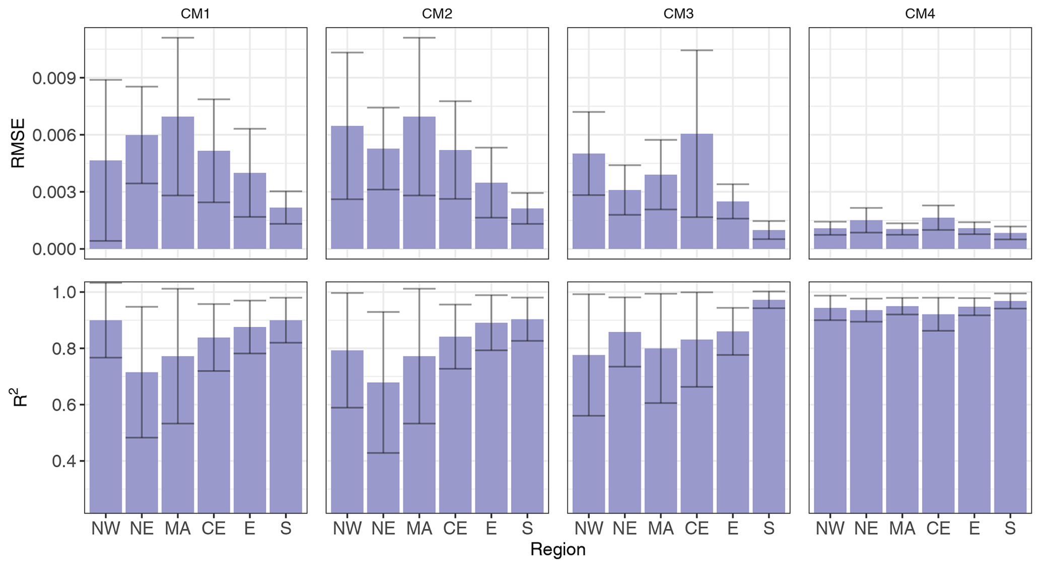
Figure 6Performance metrics (RMSE and R2) of the regression random forest model when performing a repeated 10-fold cross-validation using all the data. All counting methods are shown. The error bars show the standard deviation of these metrics.
3.2 Random forest analysis
3.2.1 Cross-validation analysis
The performance of the regression random forest models is shown in Fig. 6. RMSE values ranged from 0.0008 to 0.007 across all counting methods. Since impact occurrences were normalised in this analysis, these values should be interpreted as a fraction of the total number of the impact occurrences for each model. Overall, R2 values ranged from 0.68 to 0.97; this meant that the models explained the variance observed relatively well. However, when interpreting these results, one must note that a metric such as RMSE is expected to be small. This is because (as explained further in this section) the models tended to underpredict the number of DIOs. We need to consider that the time series of occurrences does not contain a lot of DIOs compared to the (larger) number of time steps with zero DIOs. The RMSE is expected to be relatively small, especially because the model is good at not predicting DIOs when there are none (high specificity) and because there were more actual DIOs than those predicted.

Figure 7Performance metrics (recall, precision, F score, and AUC) of the classification random forest model when performing a repeated 10-fold cross-validation using all the data. All counting methods are shown. The error bars show the standard deviation of these metrics.
In Fig. 7 we assess the performance of the classification of random forests. The classification model outputs predictions as either probabilities for each class or directly outputs the class. For this reason, the performance measures are different than in Fig. 6. We see that, generally, the precision of all models was higher than the recall. This means that the models predicted fewer than actual impact occurrences (low/moderate recall), but the predictions of impact occurrences were usually correct (high precision). In other words, the model had a low false positive rate and a slightly higher false negative rate. Moreover, recall generally appeared to be highest for the models with more balanced data sets; this was not the case for precision. AUC values were very high for all models (>0.95). However, this seems to be because specificity values were very high when compared to sensitivity values, and AUC is based on both of these measures. This means that there were very few incorrect predictions of DIOs, and there were more DIOs than those predicted.
Precision values were very high for all the models; when the models predicted an impact occurrence, the predictions were correct for 97 %–100 % of the time. Recall values varied more than precision between regions, and the standard errors were higher. However, all models predicted at least 62 % and up to 98 % of the impact occurrences. Since the F score metric combines both precision and recall, we used this measure to conclude that the best-performing counting method was the one with the least censoring criteria. However, the rest of the methods had very similar average F scores, and their censoring level did not notably affect their F scores. Furthermore, the results from the two most censoring counting methods showed that the three regions with the largest number of impact occurrences showed higher recall values than the rest of the regions. The precision across the different sub-regions did not show much variation. These regions also showed the best performance overall when using the regression models (Fig. 6). This suggests that, in order to have models with better skill and especially better recall, we need data sets with a greater number of impact occurrences, which means longer impact time series. When interpreting the model performance metrics in Figs. 6, 7, and 8, one must be aware that a new model was run each time (for each plot), which was tuned using the corresponding performance metric (see Sect. S1 for further details).
When comparing counting methods, we also found that a small sample size (low numbers of impact occurrences) limits the model's performance. We found that, generally, the less strict the censoring criteria, the better the model performance; this is displayed in Figs. 6 and 7. When using the classification models, the balance between the two class types affected model performance; the more balanced the class type is, the better the performance will be. However, although the least censoring method shows the best performance, this method could be excluding specific indicator–impact links at the NUTS-1 level, since this method counts impacts that affected the whole country as impacts that occurred independently in all sub-regions. This shows that the choice of a counting method is important when modelling impacts and can significantly affect model performance.
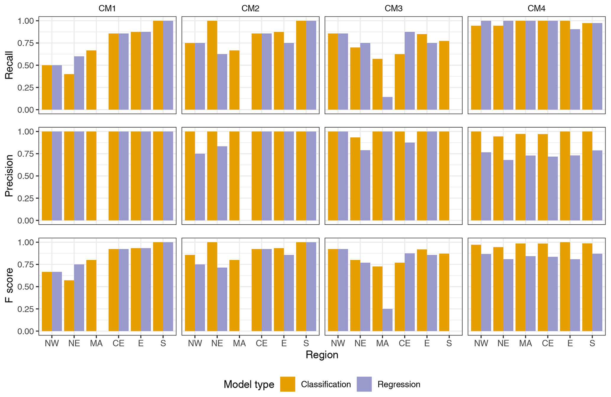
Figure 8Performance metrics (recall, precision, and F score) of the random forest models when training and validating the models on 75 % and 25 % of the data. All counting methods are shown. The regression model test predictions were converted into binary outcomes using a threshold of 1.25 DIOs.
3.2.2 Comparison of regression and classification models using a train–test analysis
Figure 8 shows the performance of the regression and classification random forest models after being trained and tested on 75 % and 25 % of the data, respectively. To do this, the regression model's output was converted to the categorical classes of impact or no impact. We tested different thresholds to convert the model outputs and found that, when the threshold was lowered, the recall increased, and the precision decreased. The opposite happened when the threshold was increased. We tested the following thresholds: 0.5, 1, 1.25, and 1.5. Model performance in this analysis was found to be slightly worse than in the cross-validation analysis. It is important to note that model performance for a region can vary, depending on how the data are partitioned for testing and training the model. Hence, model performance does not only depend on the strengths between the predictor and the response variable but also on the particular splitting. For instance, if an important event or pattern remains in the testing set, it will not be used in the training of the model; hence, it will decrease the model's predictive ability.
Although classification models appear to be better at predicting impact events in this analysis, these models did not contain any information on impact severity, whereas regression models did. Since both the model types performed well, we suggest further evaluation of these to predict impacts, for example, by using a classification model with more classes (to represent different impact severities) or using a different threshold to divide the two classes in this study. Also, similar to the previous cross-validation analysis (Sect. 3.1), here we see more clearly that, overall, regions with a higher number of total impact occurrences performed best here; these are the S, CE, and E regions.

Figure 9Predictor importance when using the regression random forest models and the two most censoring counting methods. The top 10 predictors for each counting method and sub-region are shown.
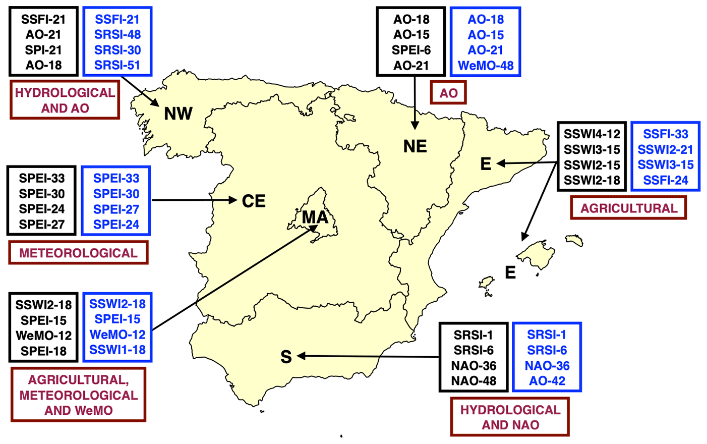
Figure 10Map with the top four predictors for each sub-region when using the regression random forest models and the two most censoring counting methods, in blue and black, respectively. The best type of predictors for each sub-region are in red.
3.3 Predictor importance
Figure 9 shows the predictor importance using the two most censoring counting methods and regression random forest models. The overall patterns of predictor importance did not change significantly when we compared them to the classification models (not shown). This, and the fact that both regression and classification models showed similar performance (Sect. 3.2.2), also confirms that the discussed potential bias in reporting culture over time does not seem to affect our random forest results. The top predictors for each region are summarised in Fig. 10.
Overall, the meteorological indicator, SPEI, was a top predictor in the CE and MA, at timescales between 24–33 and 15–18 months, respectively. In the E and in MA, agricultural indices were top predictors at timescales of 12–21 and 18 months, respectively. The hydrological indicator, SSFI, was a top predictor in the NW at a timescale of 21 months. The other hydrological indicator, SRSI, was a top predictor in the S region, at timescales of 1–6 months. Out of all the teleconnection patterns, AO, NAO, and WeMO were the top predictors, with the AO in the NW and NE at timescales between 15–21 months, the NAO in the S region between 36–48 months, and the WeMO in MA aggregated at 12 months.
We found that both analyses (correlation strength and random forest variable importance) tended to show similar predictor importance results in most sub-regions. When assessing the best drought indicators using both methods, the MA, CE, E, and S regions showed similar results. For the climate indices, the NE, followed by the S, showed the most agreement. These results indicate that, for these top predictors, the indicator–impact relationship is linear.
The results presented here are based on the most censoring counting methods (CM1 and CM2), since these showed the highest correlation strengths in the correlation analysis. Even though these two methods showed a lower predictive skill in the random forest models, we attribute this to the reduced number of impact occurrences. If we compare these results to the ones using CM3, the results remain mostly the same in half of the regions. We excluded CM4 from this analysis.
3.4 Drought vulnerability analysis
Including drought vulnerability factors when modelling drought impacts has been shown to increase model performance (Blauhut et al., 2016); however, because most of the vulnerability factors studied here (e.g. GDP per capita, public water supply, unemployment, GVA by industry except construction, agriculture, forestry, and fishing, and by all NACE activities) were only available starting from the years 1999 or 2000, models built with these factors were not as robust as the rest of our models. Therefore, we cannot assume that the results found would reproduce themselves for the rest of the study period.
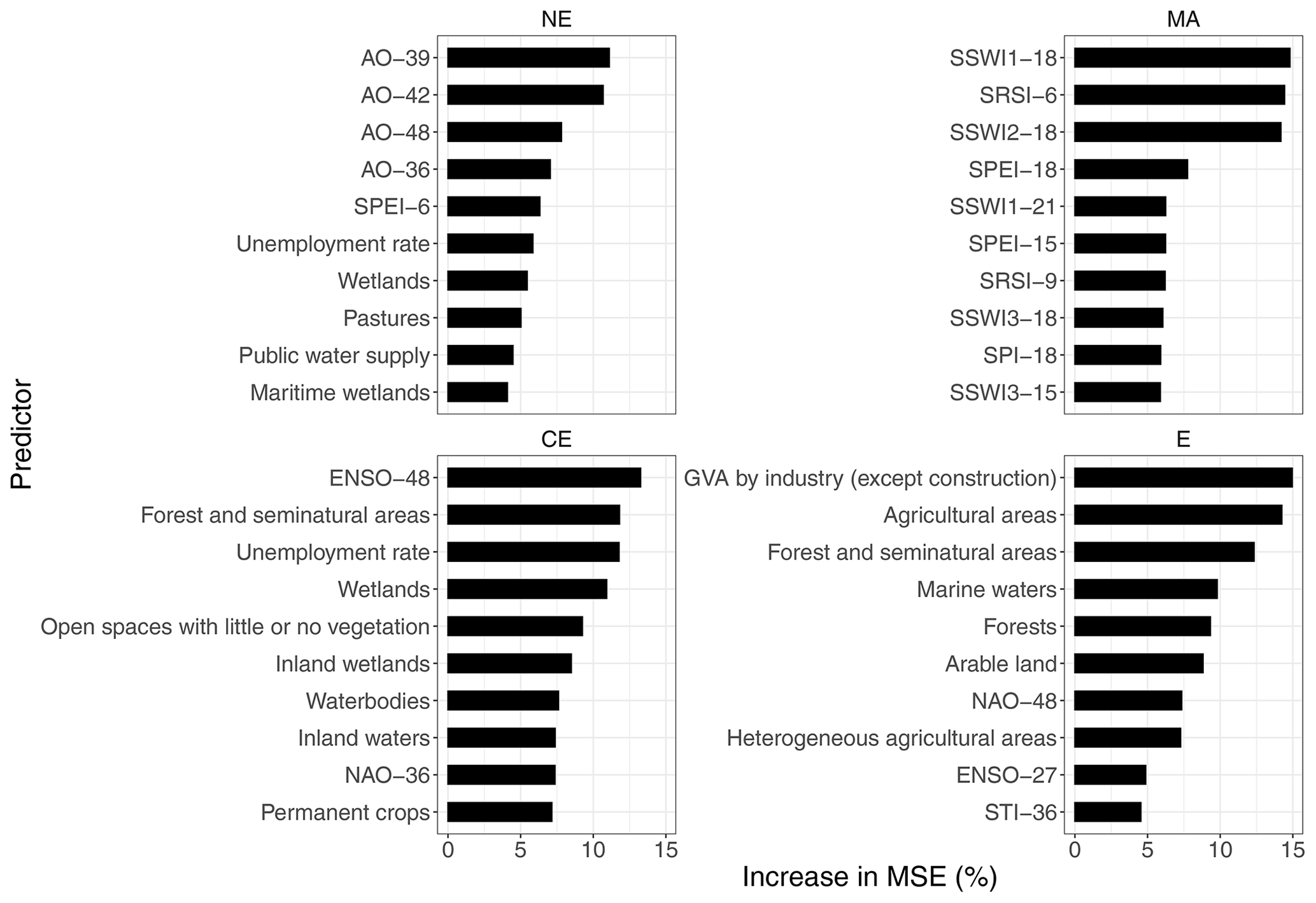
Figure 11Predictor importance when using regression random forest models built with vulnerability factors in addition to the drought indices. Counting method CM1 is used. Models are built with data from 2000–2012.
However, from an exploratory analysis, we find that vulnerability factors, in particular the land cover types of forest and seminatural areas and agricultural areas, and factors, such as unemployment rate and GVA by industry (except construction), do increase the accuracy of the models when they are included in especially two regions (CE and E). Also, the exclusion of the drought indices does not substantially decrease the model performance in either the regression or classification random forest models. Therefore, we conclude that including drought vulnerability factors, in some cases, does seem to improve the accuracy of some models. This is shown in the variable importance results (Fig. 11). Regions that had very few DIOs (NW and S) were not considered in this analysis. Since this analysis is limited by the availability of vulnerability data (the period studied here missed the first two drought events), we cannot assume that these conclusions hold true for our main results, especially considering that these models are not as robust.
In this study, we systematically investigated the link between drought impacts in Spain and drought indicators and teleconnection patterns. We also investigated the potential for vulnerability factors to be used as impact drivers. This means that we used a hybrid data approach, as defined by Blauhut (2020), to investigate drought risk as a function of hazard indicators, exposure and vulnerability factors, and impact information using a statistical model. We found significant links between the drought indicators and climate indices, and drought impact reports from the EDII database. We assessed these links by, first, using a correlation analysis and, second, by modelling drought impacts using drought indicators and teleconnection patterns as predictors in a random forest model. While random forest models seemed to be limited by the amount of impact occurrence data, they were skilful in predicting drought impact occurrences. Furthermore, we have shown that using drought impact reports from the EDII with a random forest model for Spain, a region with a reduced number of impact report entries, already provides good predictability of impacts for several sub-regions, making us confident in the robustness of our results. Drought impact information from this database has already been successfully linked to drought hazards and shown to have potential for impact forecasting (Blauhut et al., 2015, 2016; Stagge et al., 2015; Sutanto et al., 2019; Bachmair et al., 2015, 2016b); it also proves to be useful here when assessing links between different drought indicators and impacts.
We found strong and significant correlations between drought indicators and reported impacts in most regions. We also found spatial differences in indicator–impact correlations. Out of all the indices, the SPI (followed by SPEI) showed the strongest correlations overall and significant correlations in all regions. Therefore, we recommend the use of these indicators if only one indicator is to be used for predictive purposes. These meteorological indices have already been linked to drought impacts in Spain or the Mediterranean region in several studies. For example, the SPI has been used to successfully forecast above-normal summer wildfire activity (Gudmundsson et al., 2014). The SPEI has been used to detect drought impacts on vegetation activity (Gouveia et al., 2017), and the SPI has been correlated to tree ring widths to determine the impacts of drought on forest growth (Pasho et al., 2011).
When comparing the most important predictors from both analyses (correlation strength and random forest variable importance), we found a general agreement for most sub-regions. In the random forest analysis, the top predictors for each region were the SSFI and AO in the NW, AO in the NE, SSWI1-2, SPEI and WeMO in MA, SPEI in the CE, SSWI2-4 in the E, and SRSI and NAO in the S region (see Fig. 10). Our results show strong links between impacts and drought indices and teleconnection patterns. Drought and its links to teleconnection patterns is studied well in the literature (see Sect. 2.2); however, links between EDII impacts and teleconnection patterns have not been investigated before, and here we show that, in some regions, they are better predictors of drought impacts than commonly used drought indices.
By including the STI we also investigated links between temperature and impact occurrences. The correlation results showed mainly positive and significant correlations, which suggest a relationship between these two variables. However, the STI neither showed the strongest correlations nor greatest variable importance (in the random forest analysis) when compared to other drought indicators or teleconnection patterns, except for the NE region, where it showed higher correlation strengths than the rest of the indicators. Although we do not recommend the use of this index as a single drought predictor, we believe that its observed connection to drought impacts is important and might become more important as temperatures in Spain continue to increase, especially since there already is evidence of increasing trends in evapotranspiration in most meteorological stations in Spain due to decreased relative humidity and increased maximum temperature that has occurred since the 1960s (Vicente-Serrano et al., 2014a). Moreover, González-Hidalgo et al. (2018) pointed out that, since 1990, the role of atmospheric evaporative demand has been playing a large role in drought development. They state that drought is being driven by temperature conditions that affect atmospheric evaporative demand independently of precipitation evolution. In our study, the SPEI, which includes the effects that temperature has on evapotranspiration, showed higher correlations than the SPI in four out of six regions (NW, NE, CE, and E), which again suggests that including the effects of temperature when investigating drought and its impacts is important.
Adequate drought management requires knowledge of the time that different drought types take to propagate through different water resource systems. Both of our analyses mostly agreed on the timescales at which different types of drought started to cause impacts. The timescales that showed the strongest links with impact occurrences depended on the sub-region and the method for its analysis. However, using both analyses, we found the strongest links overall to be at timescales between 15–33 months for the meteorological indices, between 6–33 months for the hydrological indicator SSFI, between 1–18 months for the hydrological indicator SRSI, and between 6–21 months for layers 1–3 of the agricultural index. For the deepest soil layer, the correlation analysis showed strongest correlations at shorter timescales, i.e. from 1–9 months. The timescales at which the meteorological indices showed the strongest links were usually longer than those found in Germany and similar to the UK (Bachmair et al., 2016b). In these regions, SPI and SPEI showed the best links with impact occurrences at accumulation periods of 12–24 months for the UK and at accumulation periods of 2–4 months for Germany. Stagge et al. (2015) found that Norway, Bulgaria, and Slovenia responded even more rapidly to meteorological drought than Germany and the UK, which shows that Spain has the longest impact response out of these countries.
Furthermore, our results show that systems that respond to precipitation anomalies at the shortest timescales take longer to propagate to impacts. For instance, we have shown that the meteorological indices correlated with impacts at long timescales. The agricultural index in the top three layers (1–3) showed correlations at long timescales. Viewed differently, the hydrological index showed strong correlations overall at the earliest timescales. In our analysis, this indicates that drought impacts respond to hydrological droughts faster than meteorological and shallow layer soil moisture droughts. This drought propagation chain has been suggested by Van Loon and Laaha (2015), who detected propagation signals from meteorological to hydrological droughts. Our results indicate that if we want to predict drought impacts at short timescales, we should use hydrological drought indices.
The agricultural index showed more significant and negative correlations in the two shallowest soil layers. A weaker link between lower layer soil moisture and drought impacts can be explained by the fact that the soil moisture content of these layers, which are usually below the root zone of most crops, has a slower and more aggregated behaviour. Aggregating these indices then creates a more averaged time series with fewer anomalies, which then leads to lower correlations. The agricultural indicator also revealed an anomalous pattern in the NE region; it showed positive and significant correlations at all soil depths. This may be explained by a lower exposure to drought due to lower population density, which also explains the weaker indicator–impact correlations shown by the meteorological and hydrological drought indicators. However, this pattern may also be (partly) explained by the fact that this region reported drought impact occurrences in July–October 2009 (see Fig. 3), a period in which there were no reports in other regions. A region can still be suffering from drought impacts during a period where precipitation levels are above the climatological mean due to long-lasting impacts of a previous drought (e.g. Boletín Oficial del Estado, 2009) and, hence, results in positive (or weak negative) correlations.
Spain's resilience to short-term droughts, due to its extensive network of hydraulic reservoirs, could explain why we found most indicator–impact links at long timescales (especially meteorological indicators and teleconnection patterns). We found that most of the links between meteorological indicators and teleconnection patterns, and impact occurrences were strongest at timescales between 1–3 years and 1–4 years, respectively, depending on the specific indicator and sub-region. As mentioned earlier, drought conditions that last more than 2 or 3 years have been shown to limit the capacity of Spain's hydraulic infrastructures (González-Hidalgo et al., 2018). In addition to reservoir systems, groundwater storage also provides resilience (water supply to satisfy demands) during periods of drought. Therefore, groundwater droughts may play a role and be an additional factor that contributes to these long accumulation periods. Especially since 15 %–20 % of all water used in Spain is provided by groundwater (Hernández-Mora et al., 2003).
It is important to note that considering that there are not many drought events within the study period and that impacts are often clustered due to the nature of drought events, the observed tendency for longer aggregation periods to show stronger links to impacts can also be attributed to the methods used. This could be due to (or partly due to) aggregated indices being more smoothed out and consequently extending the periods that are above and below the normal.
The most frequent types of reported impacts were agriculture and livestock farming and public water supply (Fig. 1). Both of these sectors depend on reservoir systems for storing water, since irrigation and public water supply are the two sectors that consume most of the stored water from reservoirs. Our results show that SRSI is the best predictor of impacts, outperforming all other indicators, in the S region. The correlation analysis also showed strong and significant correlations between SRSI and impacts for several regions. This suggests that drought impacts in Spain depend on reservoir resilience, and this could explain why it takes a long time for precipitation anomalies to propagate to impacts (and the response to less frequent but longer drought periods). Reservoir storage has been shown to respond to anomalies in SPI and SPEI at long timescales in some Spanish regions (Vicente-Serrano and López-Moreno, 2005; Lorenzo-Lacruz et al., 2010). This further demonstrates that, to understand drought impacts at local scales, we need to consider the effects of local reservoir systems in addition to studying other water resource systems.
The accuracy of our results is dependent on the accuracy of the impact data used which is, specifically, the method of quantification, the completeness of the data, and potential sources of error. Since many impact reports were incomplete and their quantification is subjective, we tested four different versions of counting methods and investigated whether they had an effect on the results. We mainly tested (1) whether to count an impact that affects the entire country equally as if it only occurred in one sub-region and (2) whether and how to count impacts that lacked information on the start or end date of the impact report. In the correlation analysis, different counting methods mainly produced differences in the strength of the correlations. The least censoring counting methods showed weaker correlations overall, and significant correlations disappeared in one-third of the regions. However, in the random forest analysis, the least censoring counting methods produced models with higher predictive skill than the more censoring counting methods. Regions with the most impact data also performed best. We infer that this is because the performance of a random forest model highly depends on the quantity of data used for its training. We therefore conclude that, when working with impact data, it is important to compare counting methods and to investigate their effect on the results to overcome potential biases due to subjectivity.
The vulnerability analysis revealed that some vulnerability factors may also be appropriate drought impact drivers. When we compare our vulnerability analysis results to the results from Blauhut et al. (2016), who investigated drought risk in Europe using vulnerability factors and drought hazard indices, we find some similarities. For instance, they found that, for the western Mediterranean region, some of the best performing vulnerability factors included the area of agriculture, seminatural areas, and wetlands. These results agree with our findings (see Fig. 11). They also did not find factors such as GDP per capita or public water supply to be good predictors. They also showed that, overall, vulnerability factors improved model accuracy.
The results of this study are limited by the availability of drought impact data because there was just a small number of impact occurrences recorded for each drought event (when compared to other countries) and because the data used only covered events until 2013. A later major drought event (2017–2018) was not included because those data are, so far, not publicly available and quality checked. Therefore, we encourage future studies to (1) focus on conducting sector-specific analyses of impacts (e.g. Blauhut et al., 2015, 2016; Stagge et al., 2015; Bachmair et al., 2016b), (2) explore different types of impact data, for instance, agricultural and economic data (e.g. Sainz de la Maza and Del Jesús, 2020), and (3) model exposure and vulnerability (in addition to drought hazard) to understand how future drought risk will change (Blauhut, 2020).
The R package randomForest is available at https://cran.r-project.org/web/packages/randomForest/randomForest.pdf (Liaw and Wiener, 2002). The R package caret is available at https://doi.org/10.18637/jss.v028.i05 (Kuhn, 2008). The R package panas is available at https://github.com/matteodefelice/panas/ (De Felice, 2020). The R package SPEI is available at http://sac.csic.es/spei (Beguería and Vicente-Serrano, 2014). The Standardised Drought Analysis Toolbox (SDAT) is available at http://amir.eng.uci.edu/software.php (Hao et al., 2014; Farahmand and AghaKouchak, 2015a, b). The research data used in this study are all publicly accessible. The precipitation and temperature data sets used are available at http://hdl.handle.net/10261/183071, last access: 5 March 2022 (Gutiérrez et al., 2019; Herrera et al., 2019). Data for streamflow and reservoir levels are available at https://sig.mapama.gob.es/redes-seguimiento/index.html?herramienta=Aforos (Ministerio para la Transición Ecológica y el Reto Demográfico, 2022). Volumetric soil water content data from the ERA5-Land data set are available at https://doi.org/10.24381/cds.68d2bb30 (Muñoz Sabater, 2019). Data for the climate indices of NAO, EA, AO, and ENSO, from the NOAA Climate Prediction Center, are available at https://psl.noaa.gov/data/climateindices/list/ (NOAA, 2021a) and https://www.cpc.ncep.noaa.gov/data/teledoc/ea.shtml (NOAA, 2021b), and the data for the WeMO are available at http://www.ub.edu/gc/wemo/ (Martin-Vide and Lopez-Bustins, 2006). The data for the drought vulnerability factors are available at https://www.ine.es (Instituto Nacional de Estadística, 2022a, b, c), https://ec.europa.eu/eurostat/ (Eurostat, 2022a, b, c, d) and https://land.copernicus.eu/pan-european/corine-land-cover (European Environment Agency, 2022). The results from the cross-validation analysis and an explanation on how to tune the random forest models can be obtained at https://doi.org/10.5281/zenodo.6322803 (Torelló-Sentelles, 2022).
The supplement related to this article is available online at: https://doi.org/10.5194/hess-26-1821-2022-supplement.
HTS and CLEF contributed to the design of the study, the interpretation of the results, and the writing of the paper. HTS performed the analysis and prepared the paper.
The contact author has declared that neither they nor their co-author has any competing interests.
Publisher's note: Copernicus Publications remains neutral with regard to jurisdictional claims in published maps and institutional affiliations.
We thank the two reviewers, Claudia Teutschbein and Veit Blauhut, for their helpful and constructive comments. We thank the following data providers: the European Drought Impact Report Inventory database, Ministerio para la Transición Ecológica y el Reto Demográfico, NOAA Climate Prediction Center, Copernicus Climate Change Service (C3S) Climate Data Store, DIGITAL.CSIC, Instituto Nacional de Estadística, Eurostat, Copernicus Land Monitoring Service and EM-DAT, the Emergency Events Database, Université Catholique de Louvain (UCL) – CRED, and Debarati Guha-Sapir (https://www.emdat.be/, last access: 1 April 2021), Brussels, Belgium, for providing us with the data. We also thank Sophie Bachmair, for her initial technical help and suggestions.
This work has been supported by the ClimXtreme project funded by the German Federal Ministry for Education and Research (BMBF) and by the Institute for Basic Science (IBS), Republic of Korea (grant no. IBS-R028-D1).
This paper was edited by Micha Werner and reviewed by Veit Blauhut and Claudia Teutschbein.
Austin, R., Cantero-Martínez, C., Arrúe, J., Playán, E., and Cano-Marcellán, P.: Yield–rainfall relationships in cereal cropping systems in the Ebro river valley of Spain, Eur. J. Agron., 8, 239–248, https://doi.org/10.1016/S1161-0301(97)00063-4, 1998. a
Bachmair, S., Kohn, I., and Stahl, K.: Exploring the link between drought indicators and impacts, Nat. Hazards Earth Syst. Sci., 15, 1381–1397, https://doi.org/10.5194/nhess-15-1381-2015, 2015. a, b, c, d
Bachmair, S., Stahl, K., Collins, K., Hannaford, J., Acreman, M., Svoboda, M., Knutson, C., Smith, K. H., Wall, N., Fuchs, B., Crossman, N. D., and Overton, I. C.: Drought indicators revisited: the need for a wider consideration of environment and society: Drought indicators revisited, Wiley Interdiscip. Rev.: Water, 3, 516–536, https://doi.org/10.1002/wat2.1154, 2016a. a, b, c, d
Bachmair, S., Svensson, C., Hannaford, J., Barker, L. J., and Stahl, K.: A quantitative analysis to objectively appraise drought indicators and model drought impacts, Hydrol. Earth Syst. Sci., 20, 2589–2609, https://doi.org/10.5194/hess-20-2589-2016, 2016b. a, b, c, d, e, f, g
Bachmair, S., Svensson, C., Prosdocimi, I., Hannaford, J., and Stahl, K.: Developing drought impact functions for drought risk management, Nat. Hazards Earth Syst. Sci., 17, 1947–1960, https://doi.org/10.5194/nhess-17-1947-2017, 2017. a
Beguería, S., Vicente-Serrano, S. M., Reig, F., and Latorre, B.: Standardized precipitation evapotranspiration index (SPEI) revisited: parameter fitting, evapotranspiration models, tools, datasets and drought monitoring, Int. J. Climatol., 34, 3001–3023, https://doi.org/10.1002/joc.3887, 2014. a
Beguería, S. and Vicente-Serrano, S. M.: Calculation of the Standardised Precipitation-Evapotranspiratoin Index, CRAN [code], http://sac.csic.es/spei (last access: 5 April 2022), 2017. a
Blauhut, V.: The triple complexity of drought risk analysis and its visualisation via mapping: a review across scales and sectors, Earth-Sci. Rev., 210, 103345, https://doi.org/10.1016/j.earscirev.2020.103345, 2020. a, b
Blauhut, V., Gudmundsson, L., and Stahl, K.: Towards pan-European drought risk maps: quantifying the link between drought indices and reported drought impacts, Environ. Res. Lett., 10, 014008, https://doi.org/10.1088/1748-9326/10/1/014008, 2015. a, b
Blauhut, V., Stahl, K., Stagge, J. H., Tallaksen, L. M., De Stefano, L., and Vogt, J.: Estimating drought risk across Europe from reported drought impacts, drought indices, and vulnerability factors, Hydrol. Earth Syst. Sci., 20, 2779–2800, https://doi.org/10.5194/hess-20-2779-2016, 2016. a, b, c, d, e, f
Boletín Oficial del Estado: Real Decreto 14/2009, de 5 de diciembre, por el que se adoptan medidas urgentes para paliar los efectos producidos por la sequía en determinadas cuencas hidrográficas, Boletín Oficial del Estado, 293, 103532–103544, https://www.boe.es/boe/dias/2009/12/05/pdfs/BOE-A-2009-19563.pdf, 2009. a
Breiman, L.: Random Forests, Mach. Learn., 45, 5–32 https://doi.org/10.1023/A:1010933404324, 2001. a, b
Cardona, O. D., Van Aalst, M. K., Birkmann, J., Fordham, M., Mc Gregor, G., Rosa, P., Pulwarty, R. S., Schipper, E. L. F., and Sinh, B. T.: Determinants of risk: exposure and vulnerability, in: Managing the risks of extreme events and disasters to advance climate change adaptation. A Special Report of Working Groups I and II of the Intergovernmental Panel on Climate Change, IPCC, Cambridge University Press, 65–108, 2012. a
Cutler, A., Cutler, D. R., and Stevens, J. R.: Random Forests, in: Ensemble Machine Learning: Methods and Applications, edited by Zhang, C. and Ma, Y., Springer US, Boston, MA,, 157–175, https://doi.org/10.1007/978-1-4419-9326-7_5, 2012. a, b
Davis, J. and Goadrich, M.: The relationship between Precision-Recall and ROC curves, in: Proceedings of the 23rd international conference on Machine learning, Association for Computing Machinery, Pittsburgh, Pennsylvania, USA, 15 June 2006, 233–240 https://doi.org/10.1145/1143844.1143874, 2006. a, b
De Felice, M.: Reduce the friction when working with maps and time-series, GitHub [code], https://rdrr.io/github/matteodefelice/panas/ (last access: 9 April 2021), 2020. a, b
del Moral, L. and Hernandez-Mora, N.: La experiencia de sequías en España: inercias del pasado y nuevas tendencias en la gestión de riesgos, in: 5∘ Water Governance International Meeting, Water Governance Practices under Water Scarcity, Universidade de São Paulo, São Paulo, Brazil, 10–13 November 2015, 2015. a
del Moral, L. and Saurí, D.: Changing Course: Water Policy in Spain, Environment: Science and Policy for Sustainable Development, 41, 12–15, https://doi.org/10.1080/00139159909604640, 1999. a
Estrela, T. and Vargas, E.: Drought Management Plans in the European Union. The Case of Spain, Water Resour. Manage., 26, 1537–1553, https://doi.org/10.1007/s11269-011-9971-2, 2012. a
European Environment Agency: CORINE Land Cover (CLC), Copernicus Services [data set], https://land.copernicus.eu/pan-european/corine-land-cover (last access: 12 November 2021), 2022. a
Eurostat: https://ec.europa.eu/eurostat/web/nuts/background, last access: 12 February 2020. a
Eurostat: Your key to European statistics, https://ec.europa.eu/eurostat/, last access: 5 April 2022a. a
Eurostat: Unemployment rates by sex, age, educational attainment level and NUTS 2 regions (%), eurostat Data Browser [data set], http://appsso.eurostat.ec.europa.eu/nui/show.do?lang=en&dataset=lfst_r_lfu3rt, last access: 5 April 2022b. a
Eurostat: Population density by NUTS3 region, eurostat Data Browser [data set], https://ec.europa.eu/eurostat/databrowser/view/DEMO_R_D3DENS/default/table?lang=en&category=reg.reg_dem.reg_dempoar, last access: 5 April 2022c. a
Eurostat: Gross value added at basic prices by NUTS 3 regions, eurostat Data Browser [data set], http://appsso.eurostat.ec.europa.eu/nui/show.do?dataset=nama_10r_3gva, last access: 5 April 2022d. a
Farahmand, A. and AghaKouchak, A.: A generalized framework for deriving nonparametric standardized drought indicators, Adv. Water Resour., 76, 140–145, https://doi.org/10.1016/j.advwatres.2014.11.012, 2015a. a, b
Farahmand, A. and AghaKouchak, A.: Standardized Drought Analysis Toolbox (SDAT) Software Package, [code], http://amir.eng.uci.edu/software.php (last access: 5 April 2022), 2015b. a
Feldstein, S. B. and Franzke, C.: Are the North Atlantic Oscillation and the northern annular mode distinguishable?, J. Atmos. Sci., 63, 2915–2930, https://doi.org/10.1175/JA3798.1, 2006. a
Feldstein, S. B. and Franzke, C. L. E.: Atmospheric Teleconnection Patterns, in: Nonlinear and Stochastic Climate Dynamics, edited by Franzke, C. L. E. and O'Kane, T. J., Cambridge University Press, Cambridge, 54–104, https://doi.org/10.1017/9781316339251.004, 2017. a
Gimeno, L., Ribera, P., Iglesias, R., de la Torre, L., García, R., and Hernández, E.: Identification of empirical relationships between indices of ENSO and NAO and agricultural yields in Spain, Clim. Res., 21, 165–172, https://doi.org/10.3354/cr021165, 2002. a
González-Hidalgo, J. C., Vicente-Serrano, S. M., Peña-Angulo, D., Salinas, C., Tomas-Burguera, M., and Beguería, S.: High-resolution spatio-temporal analyses of drought episodes in the western Mediterranean basin (Spanish mainland, Iberian Peninsula), Acta Geophys., 66, 381–392, https://doi.org/10.1007/s11600-018-0138-x, 2018. a, b, c, d
Gouveia, C., Trigo, R., Beguería, S., and Vicente-Serrano, S.: Drought impacts on vegetation activity in the Mediterranean region: An assessment using remote sensing data and multi-scale drought indicators, Global Planet. Change, 151, 15–27, https://doi.org/10.1016/j.gloplacha.2016.06.011, 2017. a
Gudmundsson, L. and Seneviratne, S. I.: Anthropogenic climate change affects meteorological drought risk in Europe, Environ. Res. Lett., 11, 044005, https://doi.org/10.1088/1748-9326/11/4/044005, 2016. a
Gudmundsson, L., Rego, F. C., Rocha, M., and Seneviratne, S. I.: Predicting above normal wildfire activity in southern Europe as a function of meteorological drought, Environ. Res. Lett., 9, 084008, https://doi.org/10.1088/1748-9326/9/8/084008, 2014. a
Guha-Sapir, D., Below, R., and Hoyois, P.: EM-DAT: the CRED/OFDA international disaster database, Université Catholique de Louvain [data set], https://www.emdat.be/ (last access: 1 April 2021), 2016. a
Gutiérrez, J. M., Herrera, S., Cardoso, R. M., Soares, P. M. M., Espírito-Santo, F., and Viterbo, P.: Iberia01: Daily gridded (0.1∘ resolution) dataset of precipitation and temperatures over the Iberian Peninsula, DIGITAL.CSIC [data set], https://doi.org/10.20350/DIGITALCSIC/8641, http://hdl.handle.net/10261/183071 (last access: 5 March 2022), 2019. a, b
Guttman, N. B.: Accepting the Standardized Precipitation Index: a calculation algorithm, JAWRA J. Am. Water Resour. Assoc., 35, 311–322, https://doi.org/10.1111/j.1752-1688.1999.tb03592.x, 1999. a
Hao, Z. and AghaKouchak, A.: A Nonparametric Multivariate Multi-Index Drought Monitoring Framework, J. Hydrometeorol., 15, 89–101, https://doi.org/10.1175/JHM-D-12-0160.1, 2014. a
Hao, Z., AghaKouchak, A., Nakhjiri, N., and Farahmand, A.: Global integrated drought monitoring and prediction system, Sci. Data, 1, 140001, https://doi.org/10.1038/sdata.2014.1, 2014. a
Hernández-Mora, N., Martínez Cortina, L., and Fornés, J.: Intensive groundwater use in Spain, in: Intensive Use of Groundwater: Challenges and Opportunities, edited by Llamas, M. and Custodio, E., Swets and Zeitlinger BV, The Netherlands, 387–414, 2003. a
Herrera, S., Cardoso, R. M., Soares, P. M., Espírito-Santo, F., Viterbo, P., and Gutiérrez, J. M.: Iberia01: a new gridded dataset of daily precipitation and temperatures over Iberia, Earth Syst. Sci. Data, 11, 1947–1956, https://doi.org/10.5194/essd-11-1947-2019, 2019. a, b
Hervás-Gámez, C. and Delgado-Ramos, F.: Drought Management Planning Policy: From Europe to Spain, Sustainability, 11, 1862, https://doi.org/10.3390/su11071862, 2019. a
Hripcsak, G. and Rothschild, A. S.: Agreement, the F-Measure, and Reliability in Information Retrieval, J. Am. Med. Inf. Assoc., 12, 296–298, https://doi.org/10.1197/jamia.M1733, 2005. a
Iglesias, A., Moneo, M., Garrote, R., and Flores, F.: Drought and climate risks, in: Water policy in Spain, edited by Garrido, A. and Llamas, R. M., 63–75, CRC Press, Cambridge, 2009. a
Iglesias, E., Garrido, A., and Gomez-Ramos, A.: Evaluation of drought management in irrigated areas, Agric. Econ., 29, 211–229, https://doi.org/10.1111/j.1574-0862.2003.tb00158.x, 2003. a
Instituto Nacional de Estadística: https://www.ine.es/, last access: 5 April 2022a. a
Instituto Nacional de Estadística: Estadística sobre el suministro y saneamiento del agua, Serie 2000–2018, INEbase [data set], https://www.ine.es/jaxi/Datos.htm?path=/t26/p067/p01/serie/l0/&file=01003.px#!tabs-tabla, last access: 5 April 2022b. a
Instituto Nacional de Estadística: PIB y PIB per cápita, Serie 2000–2020, INEbase [data set], https://www.ine.es/dyngs/INEbase/es/operacion.htm?c=Estadistica_C&cid=1254736167628&menu=resultados&idp=1254735576581#, last access: 5 April 2022c. a
Kingston, D. G., Stagge, J. H., Tallaksen, L. M., and Hannah, D. M.: European-Scale Drought: Understanding Connections between Atmospheric Circulation and Meteorological Drought Indices, J. Clim., 28, 505–516, https://doi.org/10.1175/JCLI-D-14-00001.1, 2015. a
Kuhn, M.: Building Predictive Models in R using the caret Package, CRAN [code], https://doi.org/10.18637/jss.v028.i05, 2008. a, b
Liaw, A. and Wiener, M.: Classification and regression by randomForest, R news, 2, 18–22, https://cran.r-project.org/web/packages/randomForest/randomForest.pdf (last access: 5 April 2022), 2002. a, b, c
Lorenzo-Lacruz, J., Vicente-Serrano, S., López-Moreno, J., Beguería, S., García-Ruiz, J., and Cuadrat, J.: The impact of droughts and water management on various hydrological systems in the headwaters of the Tagus River (central Spain), J. Hydrol., 386, 13–26, https://doi.org/10.1016/j.jhydrol.2010.01.001, 2010. a
Manzano, A., Clemente, M. A., Morata, A., Luna, M. Y., Beguería, S., Vicente-Serrano, S. M., and Martín, M. L.: Analysis of the atmospheric circulation pattern effects over SPEI drought index in Spain, Atmos. Res., 230, 104630, https://doi.org/10.1016/j.atmosres.2019.104630, 2019. a
Martin-Vide, J. and Lopez-Bustins, J.-A.: The Western Mediterranean Oscillation and rainfall in the Iberian Peninsula, Int. J. Climatol., 26, 1455–1475, https://doi.org/10.1002/joc.1388, 2006. a, b
Martinez‐Artigas, J., Lemus‐Canovas, M., and Lopez‐Bustins, J. A.: Precipitation in peninsular Spain: Influence of teleconnection indices and spatial regionalisation, Int. J. Climatol., 41, E1320–E1335, https://doi.org/10.1002/joc.6770, 2021. a
Mason, S. J. and Graham, N. E.: Areas beneath the relative operating characteristics (ROC) and relative operating levels (ROL) curves: Statistical significance and interpretation, Q. J. Roy. Meteorol. Soc., 128, 2145–2166, https://doi.org/10.1256/003590002320603584, 2002. a
McKee, T. B., Doesken, N. J., and Kleist, J.: The relationship of drought frequency and duration to time scales, Proceedings of the 8th Conference on Applied Climatology, Anaheim, California, USA, 17–22 January 1993, 179–183, 1993. a, b, c
Ministerio de Agricultura, Pesca y Alimentación: Recurrencia y Efectos de las Sequías, 2022. a
Ministerio de Medio Ambiente: A Preliminary Assessment of the Impacts in Spain due to the Effects of Climate Change, 2005. a
Ministerio para la Transición Ecológica y el Reto Demográfico: Redes de Seguimiento del Estado e Información Hidrológica, https://sig.mapama.gob.es/redes-seguimiento/index.html?herramienta=Aforos (last access: 12 February 2020), 2022. a, b
Ministerio para la Transición Ecológica y el Reto Demográfico: Plan Nacional de Adaptación al Cambio Climático 2021–2030, https://www.miteco.gob.es/es/cambio-climatico/temas/impactos-vulnerabilidad-y-adaptacion/plan-nacional-adaptacion-cambio-climatico/default.aspx, (last access: 5 April 2021), 2020. a
Muñoz Sabater, J.: ERA5-Land monthly averaged data from 1981 to present, Copernicus Climate Change Service (C3S) Climate Data Store (CDS) [data set], https://doi.org/10.24381/cds.68d2bb30, 2019. a, b
NOAA Climate Prediction Centre: Climate Indices: Monthly Atmospheric and Ocean Time-Series, Physical Sciences Laboratory [data set], https://psl.noaa.gov/data/climateindices/list/, last access: 2 August 2021a. a
NOAA Climate Prediction Centre: East Atlantic (EA), National Weather Service [data set], https://www.cpc.ncep.noaa.gov/data/teledoc/ea.shtml, last access: 2 August 2021b. a
Ollero Lara, A., Crespo Vergara, S. I., and Pérez Cimas, M.: Las sequías y España. La respuesta del seguro agrario a un problema intermitente, Entidad Estatal de Seguros Agrarios (ENESA), Ministerio de Agricultura, Pesca y Alimentación, 2018. a
Páscoa, P., Gouveia, C. M., Russo, A., and Trigo, R. M.: The role of drought on wheat yield interannual variability in the Iberian Peninsula from 1929 to 2012, Int. J. Biometeorol., 61, 439–451, https://doi.org/10.1007/s00484-016-1224-x, 2017. a
Pasho, E., Camarero, J. J., de Luis, M., and Vicente-Serrano, S. M.: Impacts of drought at different time scales on forest growth across a wide climatic gradient in north-eastern Spain, Agric. For. Meteorol., 151, 1800–1811, https://doi.org/10.1016/j.agrformet.2011.07.018, 2011. a
Peña-Gallardo, M., Vicente-Serrano, S. M., Domínguez-Castro, F., and Beguería, S.: The impact of drought on the productivity of two rainfed crops in Spain, Nat. Hazards Earth Syst. Sci., 19, 1215–1234, https://doi.org/10.5194/nhess-19-1215-2019, 2019. a, b
Pozzi, W., Sheffield, J., Stefanski, R., Cripe, D., Pulwarty, R., Vogt, J. V., Heim Jr., R. R., Brewer, M. J., Svoboda, M., Westerhoff, R., van Dijk, A. I. J. M., Lloyd-Hughes, B., Pappenberger, F., Werner, M., Dutra, E., Wetterhall, F., Wagner, W., Schubert, S., Mo, K., Nicholson, M., Bettio, L., Nunez, L., van Beek, R., Bierkens, M., de Goncalves, L. G. G., de Mattos, J. G. Z., and Lawford, R.: Toward Global Drought Early Warning Capability: Expanding International Cooperation for the Development of a Framework for Monitoring and Forecasting, B. Am. Meteorol., 94, 776–785, https://doi.org/10.1175/BAMS-D-11-00176.1, 2013. a
Ríos-Cornejo, D., Penas, Á., Álvarez-Esteban, R., and del Río, S.: Links between teleconnection patterns and precipitation in Spain, Atmos. Res., 156, 14–28, https://doi.org/10.1016/j.atmosres.2014.12.012, 2015. a
Rodó, X., Baert, E., and Comín, F. A.: Variations in seasonal rainfall in Southern Europe during the present century: relationships with the North Atlantic Oscillation and the El Niño-Southern Oscillation, Clim. Dyn., 13, 275–284, https://doi.org/10.1007/s003820050165, 1997. a
Rossi, G. and Cancelliere, A.: Managing drought risk in water supply systems in Europe: a review, Int. J. Water Resour. Dev., 29, 272–289, https://doi.org/10.1080/07900627.2012.713848, 2013. a
Russo, A., Gouveia, C. M., Páscoa, P., DaCamara, C. C., Sousa, P. M., and Trigo, R. M.: Assessing the role of drought events on wildfires in the Iberian Peninsula, Agric. For. Meteorol., 237–238, 50–59, https://doi.org/10.1016/j.agrformet.2017.01.021, 2017. a
Sainz de la Maza, M. and Del Jesús, M.: Análisis de sequías históricas a través de los impactos derivados, Ingeniería del agua, 24, 141, https://doi.org/10.4995/ia.2020.12182, 2020. a, b, c
Salvador, C., Nieto, R., Linares, C., Díaz, J., and Gimeno, L.: Short-term effects of drought on daily mortality in Spain from 2000 to 2009, Environ. Res., 183, 109200, https://doi.org/10.1016/j.envres.2020.109200, 2020. a
Sivakumar, M. V., Motha, R., Wilhite, D., and Wood, D.: Agricultural Drought Indices. Proceedings of an Expert Meeting, WMO, Murcia, Spain, 2–4 June 2010, 219 pp., 2011. a
Spearman, C.: The Proof and Measurement of Association Between Two Things., in: Studies in individual differences: The search for intelligence., edited by Jenkins, J. J. and Paterson, D. G., Appleton-Century-Crofts, East Norwalk, 45–58, https://doi.org/10.1037/11491-005, 1961. a
Stagge, J. H., Kohn, I., Tallaksen, L. M., and Stahl, K.: Modeling drought impact occurrence based on meteorological drought indices in Europe, J. Hydrol., 530, 37–50, https://doi.org/10.1016/j.jhydrol.2015.09.039, 2015. a, b, c, d, e
Stahl, K., Kohn, I., Blauhut, V., Urquijo, J., De Stefano, L., Acácio, V., Dias, S., Stagge, J. H., Tallaksen, L. M., Kampragou, E., Van Loon, A. F., Barker, L. J., Melsen, L. A., Bifulco, C., Musolino, D., de Carli, A., Massarutto, A., Assimacopoulos, D., and Van Lanen, H. A. J.: Impacts of European drought events: insights from an international database of text-based reports, Nat. Hazards Earth Syst. Sci., 16, 801–819, https://doi.org/10.5194/nhess-16-801-2016, 2016. a, b
Sutanto, S. J., van der Weert, M., Wanders, N., Blauhut, V., and Van Lanen, H. A. J.: Moving from drought hazard to impact forecasts, Nat. Commun., 10, 4945, https://doi.org/10.1038/s41467-019-12840-z, 2019. a, b
Svoboda, M., Fuchs, B. A., Integrated Drought Management Programme, World Meteorological Organization, Global Water Partnership, University of Nebraska–Lincoln, and National Drought Mitigation Center: Handbook of drought indicators and indices, http://www.droughtmanagement.info/handbook-drought-indicators-and-indices/ (last access: 23 March 2021), 2016. a
Thornthwaite, C. W.: An Approach toward a Rational Classification of Climate, Geographical Review, 38, 55, https://doi.org/10.2307/210739, 1948. a
Torelló-Sentelles, H.: herminiats/DroughtImpactsSpain: Drought impact links to meteorological drought indicators and predictability in Spain, Zenodo [data set], https://doi.org/10.5281/zenodo.6322803, 2022. a
Van Loon, A. and Laaha, G.: Hydrological drought severity explained by climate and catchment characteristics, J. Hydrol., 526, 3–14, https://doi.org/10.1016/j.jhydrol.2014.10.059, 2015. a
Vicente-Serrano, S. M. and López-Moreno, J. I.: Hydrological response to different time scales of climatological drought: an evaluation of the Standardized Precipitation Index in a mountainous Mediterranean basin, Hydrol. Earth Syst. Sci., 9, 523–533, https://doi.org/10.5194/hess-9-523-2005, 2005. a
Vicente-Serrano, S. M., Beguería, S., and López-Moreno, J. I.: A Multiscalar Drought Index Sensitive to Global Warming: The Standardized Precipitation Evapotranspiration Index, J. Clim., 23, 1696–1718, https://doi.org/10.1175/2009JCLI2909.1, 2010. a, b, c
Vicente-Serrano, S. M., López-Moreno, J. I., Lorenzo-Lacruz, J., Kenawy, A. E., Azorin-Molina, C., Morán-Tejeda, E., Pasho, E., Zabalza, J., Beguería, S., and Angulo-Martínez, M.: The NAO Impact on Droughts in the Mediterranean Region, Springer Netherlands, Dordrecht, 23–40, https://doi.org/10.1007/978-94-007-1372-7_3, 2011. a
Vicente-Serrano, S. M., Azorin-Molina, C., Sanchez-Lorenzo, A., Revuelto, J., Morán-Tejeda, E., López-Moreno, J. I., and Espejo, F.: Sensitivity of reference evapotranspiration to changes in meteorological parameters in Spain (1961–2011), Water Resour. Res., 50, 8458–8480, https://doi.org/10.1002/2014WR015427, 2014a. a
Vicente-Serrano, S. M., Lopez-Moreno, J.-I., Beguería, S., Lorenzo-Lacruz, J., Sanchez-Lorenzo, A., García-Ruiz, J. M., Azorin-Molina, C., Morán-Tejeda, E., Revuelto, J., Trigo, R., Coelho, F., and Espejo, F.: Evidence of increasing drought severity caused by temperature rise in southern Europe, Environ. Res. Lett., 9, 044001, https://doi.org/10.1088/1748-9326/9/4/044001, 2014b. a, b
Vicente-Serrano, S. M., Azorin-Molina, C., Peña-Gallardo, M., Tomas-Burguera, M., Domínguez-Castro, F., Martín-Hernández, N., Beguería, S., El Kenawy, A., Noguera, I., and García, M.: A high-resolution spatial assessment of the impacts of drought variability on vegetation activity in Spain from 1981 to 2015, Nat. Hazards Earth Syst. Sci., 19, 1189–1213, https://doi.org/10.5194/nhess-19-1189-2019, 2019. a
Vide, J. M.: Diez características de la pluviometría española decisivas en el control de la demanda y el uso del agua, Asoc. de Geogr. Espanoles, 18, 9–16, 1994. a
Wilhite, D.: Drought as a Natural Hazard: Concepts and Definitions, in: Drought: A Global Assessment, edited by: Wilhite, D., Drought Mitigation Center Faculty Publications, London, 3–18 pp., https://digitalcommons.unl.edu/droughtfacpub/69/ (last access: 5 April 2022), 2000. a
Wilhite, D. A. and Glantz, M. H.: Understanding: the Drought Phenomenon: The Role of Definitions, Water Int., 10, 111–120, https://doi.org/10.1080/02508068508686328, 1985. a, b, c