Delineation of discrete conduit networks in karst aquifers via combined analysis of tracer tests and geophysical data

Assessment of the karst network geometry based on field data is an important challenge in the accurate modeling of karst aquifers. In this study, we propose an integrated approach for the identification of effective three-dimensional (3D) discrete karst conduit networks conditioned on tracer tests and geophysical data. The procedure is threefold: (i) tracer breakthrough curves (BTCs) are processed via a regularized inversion procedure to determine the minimum number of distinct tracer flow paths between injection and monitoring points, (ii) available surface-based geophysical data and borehole-logging measurements are aggregated into a 3D proxy model of aquifer hydraulic properties, and (iii) single or multiple tracer flow paths are identified through the application of an alternative shortest path (SP) algorithm to the 3D proxy model. The capability of the proposed approach to adequately capture the geometrical structure of actual karst conduit systems mainly depends on the sensitivity of geophysical signals to karst features, whereas the relative completeness of the identified conduit network depends on the number and spatial configuration of tracer tests. The applicability of the proposed approach is illustrated through a case study at the Hydrogeological Experimental Site (HES) in Poitiers, France.

1 Introduction

Karst conduits in carbonate aquifers provide low-hydraulic resistance paths, which exert a strong control on the spatiotemporal propagation of pressure-head perturbations (e.g., pumping-induced drawdowns) and the transport of solutes in groundwater (Goldscheider and Drew, 2007; Worthington and Ford, 2009; Kresic, 2012; Ronayne, 2013). It is therefore advisable that karst conduit networks be explicitly represented in numerical hydrogeological models (Worthington, 2009; Saller et al., 2013; Malard et al., 2015). However, due to the relative inaccessibility of aquifers, accurate characterization of the karst network geometry is a challenging task. Even in cases where portions of the karst system can be explored and mapped by speleologists and/or cave divers (Gallegos et al., 2013; Lauber et al., 2014; Scharping et al., 2018; Vuilleumier et al., 2019), it is widely acknowledged that known and accessible karst conduits represent only a small fraction of the whole drainage network. In most karst aquifer studies, the spatial occurrence of karst conduits is only known at sparse locations corresponding to their intersection with the ground surface (sinkholes and springs) and/or with boreholes.

A number of approaches have been proposed to delineate karst networks according to their observed location. Among the methods is the generation of plausible conduit networks either through analog templates (Pardo-Igúzquiza et al., 2012; Fournillon et al., 2012; Le Coz et al., 2017) or via the simulation (mimicking) of the action of speleogenetic processes considering pre-existing rock discontinuities (fractures, bedding planes, and inception horizons), e.g., Jaquet et al. (2004), Borghi et al. (2012), and de Rooij and Graham (2017). Other approaches strive to infer the spatial distribution of karst conduits through the inversion of multiple pumping test and/or tracer test data, also referred to as hydraulic or tracer tomography (Borghi et al., 2016; Mohammadi and Illman, 2019; Fischer et al., 2020). Regardless of the method pursued, any data describing the likely occurrence and location of karst conduits in the subsurface should be supplied to a given model. Geophysical methods are appealing for this purpose because of their potential to image the subsurface in a noninvasive and quasi-continuous manner. However, the detection and mapping of karst features (conduits and/or cavities) based on geophysical surveys remains a challenging task due to their volumetrically small proportion in rock volumes that may be intrinsically associated with other types of spatial heterogeneity, e.g., sedimentary facies variations. Bechtel et al. (2007) and Chalikakis et al. (2011) reviewed the strengths and weaknesses of different geophysical methods that can be considered for locating karst features in the subsurface. To date, reported field applications of surface geophysical methods to locate known or suspected water-filled karst conduits have only been successful in regard to large-diameter (>1 m) conduits at shallow depths (<20 m), e.g., Guérin et al. (2009), Zhu et al. (2011) and Sawyer et al. (2015). Relying on geophysical surveys alone for the delineation of karst networks is therefore hardly conceivable. More generally, it has been increasingly agreed that geophysical data should be analyzed conjointly with hydrogeological data for a more accurate characterization of flow- and transport-relevant heterogeneities (Hyndman and Gorelick, 1996; Rubin and Hubbard, 2005).

In the present study, we investigate the delineation of karst conduit networks via the joint analysis of tracer test data, three-dimensional (3D) seismic images, and borehole flow measurements. To the authors' knowledge, the only previous study to map karst conduit networks based on geophysical data is that of Vuilleumier et al. (2013). In that study, two-dimensional (2D) airborne electromagnetic data were processed with the pseudogenetic karst simulator of Borghi et al. (2012). At the core of the method is the computation of the shortest paths (SPs) (minimum effort) in the heterogeneous medium depicted by geophysical surveys with a fast marching algorithm (Sethian, 1996). The above SP search is also central to the approach developed in the present study. However, our approach differs from the work of Vuilleumier et al. (2013) in three main aspects. First, instead of processing 2D electromagnetic data, we process 3D seismic data supplemented by borehole flow measurements. Second, rather than applying a single-path routing algorithm in the delineation of karst conduits between pairs of source-target locations, we adopt a multiple (alternative) path finding algorithm. The applied routing scheme allows for the mapping of diverging-converging paths, which are common in karst systems, e.g., Collon et al. (2017) and Jouves et al. (2017). Finally, interwell tracer test data are considered to maximize the information value of geophysical data. More precisely, tracer breakthrough curves (BTCs) are inverted with recently developed software (Bodin, 2020a) prior to the processing of geophysical data. BTC inversion allows us to identify the minimum number of flow paths between the tracer injection and monitoring locations, which is subsequently applied in the multiple path routing formulation.

The paper is organized as follows. Section 2 develops the method for the determination of the minimum number of distinct flow paths involved in a tracer experiment. In Sect. 3, we examine the use of geophysical data as a surrogate (proxy) for aquifer hydraulic properties and we present the multiple path finding algorithm applied to the proxy model. Section 4 illustrates the application of the proposed approach to map the conduit network within the karst aquifer at the Hydrogeological Experimental Site (HES) in Poitiers, France. A discussion and conclusions are provided in Sect. 5.

2 Assessing the minimum number of distinct flow paths involved in a tracer experiment

Artificial tracer testing is a widely adopted method for the characterization of karst aquifers. Experiments are typically conducted by injecting a tracer solution into a sinkhole or well and subsequently monitoring the tracer concentration response at one or several downstream locations, usually spring(s) or pumping well(s). In the following, we will restrict the discussion to the case of tracer tests performed using nonreactive tracer species under steady-flow conditions and with a much shorter duration of the injection signal than the mean tracer transit time. This last assumption is there to support the approximation of a pulse injection as a boundary condition in the analytical transport models used later in this work.

Given the possibly complex conduit network patterns in karst aquifers, the tracer may follow different routes between the injection and monitoring points. As a result, tracer BTCs often exhibit multiple local peaks and/or extensive backward tailing, e.g., Kübeck et al. (2013), Labat and Mangin (2015), and Barberá et al. (2018). The determination of the actual number of transport flow paths involved in a tracer experiment is a challenging task because a given flow system containing N transport flow paths may produce a BTC exhibiting 1 to N concentration peaks. The number of distinguishable peaks depends on three factors: (i) the difference between the mean travel times (advection), (ii) the variance in the travel time distribution (dispersion) along each flow path, and (iii) the relative exchange (mixing) between the flow paths. On the other hand, unimodal long-tailed BTCs do not necessarily indicate the occurrence of multiple overlapping pathway responses. The long-tail behavior of a BTC may also indicate solute mass exchange between a single flow pathway and adjacent stagnant water zones, which may reflect various features: primary rock porosity, dissolution vugs, pool volumes, fragmented rock areas, transverse dead-end conduits or fractures, etc.

We propose to assess the number of distinct tracer flow paths via an inverse modeling procedure implemented in MFIT software (Bodin, 2020a). MFIT is a BTC fitting tool that combines different analytical transport models with PEST optimization routines (Doherty, 2019a, b). The general modeling approach is based on the multiflow framework first introduced by Maloszewski et al. (1992), which assumes that the karst network structure between the injection and monitoring points can be approximated by a combination of independent one-dimensional channels (Fig. 1). The four analytical models implemented in MFIT to describe the transport process at the scale of individual channels include (i) the solution of the classical advection-dispersion equation (ADE) for an instantaneous point source (Kreft and Zuber, 1978), (ii) the solution of the ADE regarding an exponentially decaying injection pulse (Marino, 1974), (iii) the single-fracture dispersion model (SFDM) of Maloszewski and Zuber (1990), and (iv) the two-region nonequilibrium (2RNE) model of Toride et al. (1993). Both the SFDM and 2RNE models are double-porosity models that consider solute mass exchange between channels and adjacent stagnant water zones. A fundamental difference between these two models is the mathematical description of the exchange between the mobile and immobile regions, which is assumed to be governed by a first-order process in the 2RNE model and by a second-order (diffusion) process in SFDM. A complete mathematical description of these models has been provided by Bodin (2020a) and is not repeated here for conciseness. While it is acknowledged that the actual geometry of the karst conduit system experienced by a tracer could be much more complex than that depicted in Fig. 1, it is assumed that this approach allows us to capture the effects of tracer mass routing through distinct pathways. In other words, channels are not assumed to represent individual karst conduits but are rather regarded as lumped submodels of the main flow routes through the karst network.

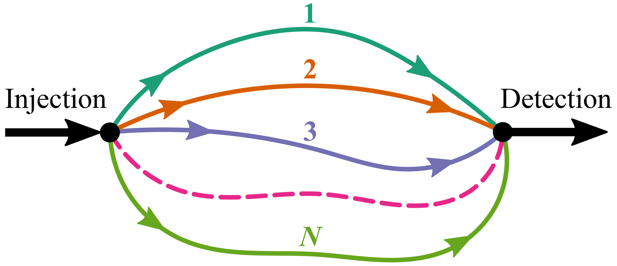
Figure 1 Schematic layout of the multiflow modeling approach implemented in MFIT software (Bodin, 2020a). The tracer transport from the injection site to the monitoring point is assumed to occur in a flow network comprising N independent one-dimensional channels.

The fitting process of a model curve to an experimental tracer BTC first requires specification of the number of channels N, followed by optimization of the model parameters pertaining to each channel. The main features of the PEST optimization algorithm are summarized below. We refer interested readers to Doherty and Hunt (2010) and Doherty (2015) for a more comprehensive presentation of theoretical concepts and associated methods, and to Bodin (2020a) for their specific implementation in MFIT software dedicated to tracer BTC fitting.

The PEST optimization routines are primarily based on the Gauss-Marquardt-Levenberg algorithm (GMLA). The objective function that is minimized during the optimization process is defined as the sum of two terms. The first term is the “measurement objective function” PHI, which is defined as the sum of the squared differences between the tracer BTC and the model-simulated curve. The second term is referred to as the “Tikhonov regularization objective function” and acts as a penalty function for deviations from some preferred parameter conditions. In the present study, we used regularization constraints that promote a solution of minimum variance for the model parameters pertaining to the different channels. The Tikhonov regularization contributes to the stability of the numerical optimization scheme, jointly with the singular value decomposition (SVD) method that removes from the estimation process the combinations of model parameters for which the tracer BTC is uninformative. Tikhonov regularization also allows us to prevent any overfitting of the tracer BTC. The regularization is controlled by a PEST variable called PHIMLIM, which defines a threshold for the objective function below which we consider that the model is calibrated. The PHIMLIM value should be congruent with both the uncertainty in the measured concentrations and the structural noise resulting from the inability of the models to perfectly simulate real-world processes. Mainly because of this last feature, it is generally not obvious to estimate a priori what is a suitable PHIMLIM value. In the present study, we used a strategy suggested by Doherty and Hunt (2010), which consists of setting PHIMLIM to a value slightly higher than the minimum objective function that can be achieved without applying regularization constraints. We chose to set PHIMLIM 15 % above the minimum value of PHI that could be obtained using 15 channels. The main cost of this method is having to perform at least two optimization runs each time: first without and then with regularization. In fact, the actual number of optimization runs is much higher because MFIT also includes a “multistart” procedure that consists of repeating the optimization process starting from different initial parameter value sets. This procedure is intended to improve the chances of converging to the global minimum of the objective function rather than a local minimum, which is a well-known potential issue with the GMLA.

The determination of the minimum number of distinct tracer flow paths between injection and monitoring points, hereafter referred to as N^*, is achieved through analysis of the curve representing the minimum PHI value obtained at different N values. The typical shape of a PHI(N) curve is that of a monotonic decreasing function converging to a horizontal asymptote, which corresponds to the PHIMLIM threshold (Fig. 2). The N^* value corresponds to the smallest value of N such that PHI(N) ≈ PHIMLIM. The N^* value is also a model-dependent parameter, as fewer channels are required to fit a long-tailed BTC with a double-porosity model (SFDM or 2RNE) rather than with the ADE instantaneous injection model.

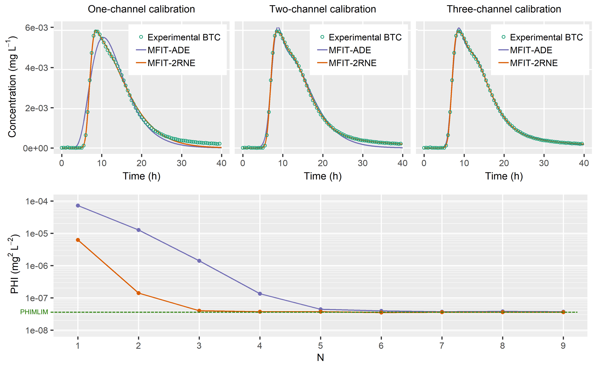
Figure 2 Example of BTC fitting analysis with the multiflow ADE and 2RNE models for different numbers of channels N. The experimental BTC corresponds to a tracer test performed in 2016 at the HES between wells M16 (injection) and M22 (pumping and observation). PHI is the fitting error objective function (sum of the squared errors between the tracer BTC and model-simulated curve) minimized with the regularization routines in PEST. The decreasing trend of the PHI(N) curves indicates the improvement in model fit with increasing number of channels N. PHIMLIM is a threshold for PHI that prevents overfitting of the tracer BTC. The optimal numbers of channels determined with the ADE and 2RNE models are $N^{*}=\mathrm{5}$ and $N^{*}=\mathrm{3}$, respectively.

3 Proxy model of the aquifer hydraulic properties and multiple path finding

Considering that karst conduits provide paths with the lowest hydraulic resistance within a given aquifer, an N^*-conduit system between a pair of tracer injection and monitoring points can be identified by searching the N^* optimal (most efficient) paths within the corresponding hydraulic conductivity field. The karst network can then be sequentially constructed by abutting and joining the subconduit systems identified based on different pairs of tracer injection and monitoring points. As our knowledge of the hydraulic conductivity field is often incomplete and uncertain, it is convenient to substitute geophysical survey data for the hydraulic conductivity field in the search for optimal paths. A necessary assumption for this approach is that a monotonic and spatially stationary relationship exists between the geophysical and hydraulic conductivity fields. However, the relationship between both parameters does not need to be explicitly modeled, which is of particular interest given the notoriously complex and site-specific nature of the problem, e.g., Pride (2006), Hyndman and Tronicke (2006), and Brauchler et al. (2012). It is beyond the scope of this paper to examine the potential strengths and weaknesses of the different existing geophysical methods for the characterization of hydrogeological heterogeneity. We refer the reader to the comprehensive review conducted by Binley et al. (2015). Of course, the reliability of the conduit networks identified with our approach largely depends on the sensitivity of geophysical measurements to karst features. It is also possible to combine different types of geophysical data into a single proxy model of aquifer hydraulic properties. In the application example presented in Sect. 4, we adopted both seismic imaging and borehole flow logging techniques.

Once a proxy model of the aquifer hydraulic properties has been established, the main challenge is the identification of the optimal paths with this model. The determination of the most efficient path between two points is a classical problem in graph theory and is commonly referred to as the SP problem. Basically, a graph is specified by a set of vertices (nodes) and a set of edges (links) connecting the vertices. Each edge is assigned a weight (cost) of traversing. This abstraction can be applied to any gridded model by mapping the vertices onto the centers of model grid cells and by connecting each vertex to its neighbors via a regular edge network. Building on the assumed (positive or negative) relationship between the geophysical and hydraulic conductivity fields, pseudolocal hydraulic resistance coefficients can be assigned to the edges as the mean (or inverse mean) geophysical property value of the two connected grid cells. A number of SP algorithms have been developed since the early 1960s, e.g., the reviews by Cherkassky et al. (1996) and Fu et al. (2006) and the recent works of Song et al. (2018) and Arslan and Manguoglu (2019). A classical and widely adopted algorithm is that of Dijkstra (1959), which was used, e.g., by Knudby and Carrera (2006) and more recently by Rizzo and de Barros (2017), in the determination of the path of least hydraulic resistance in synthetic hydraulic conductivity fields. Borghi et al. (2012) applied the fast marching algorithm of Sethian (1996) to simulate karst conduit networks as least-resistance paths based on 3D scalar grids of pseudovelocity fields empirically derived from different geological indicators. The fast marching method can be regarded as an extension of Dijkstra's method to the continuous domain. In a study parallel to that of Borghi et al. (2012), Collon-Drouaillet et al. (2012) adopted the A^* algorithm (Hart et al., 1968), which utilizes a heuristic function to guide the search process. For our purpose, we are interested not only in determining the SP between two vertices but also in determining a finite number (N^*) of distinct paths, as revealed by tracer BTC inversion. In graph theory, this problem is known as the k-shortest path (KSP) problem, and many algorithms have been proposed to solve this problem, e.g., Yen (1971), Lawler (1972), Brander and Sinclair (1996), Eppstein (1998), Hershberger et al. (2007), Scano et al. (2015), and Chondrogiannis et al. (2015, 2017) and the references therein. In the present study, we selected the OnePass+ algorithm of Chondrogiannis et al. (2015, 2017) as implemented in the Alternative Routing Library for Boost Graph (ARLib) developed by Leonardo Arcari (https://github.com/leonardoarcari/arlib, last access: 25 February 2022). The main interest of this algorithm is that it allows the user to specify a maximum overlap ratio between alternative paths. During the search process, a candidate alternative path is successively compared to the previously retained paths by computing the ratio between the sum of the weights of the shared edges and the total cost of each of the previously retained paths, omitting the starting and ending edges. The candidate path is added to the KSP solution set only if its overlap ratio is below a predefined θ threshold value between 0 and 1. Such a threshold is particularly relevant for dense graphs retrieved from a continuous geophysical model. Otherwise, the KSP search process typically results in a set of very similar paths with only minor deviations with respect to the SP. An open issue is the specification of the threshold value. As already noted, the N^* paths yielded by the inversion of tracer test data are not supposed to be as disconnected as in Fig. 1, but their overlap must nevertheless be small enough to produce a detectable signature in the BTC. Further theoretical and/or numerical investigations could be pursued to narrow, if possible, the value range of θ, but such developments are beyond the scope of the present study. Alternatively, θ may be considered a calibration parameter whose value may be adjusted to produce a good geometrical match between the computed conduit network and independently observed karst features. In the case study presented below, we adopted an empirical threshold of 0.5.

4 Case study: Hydrogeological Experimental Site (HES) in Poitiers, France

The investigations conducted at the HES focus on a confined limestone aquifer extending approximately 35 to 130 m below the ground surface. Detailed information on the hydrogeology of the site can be found in the article by Audouin et al. (2008) and is not repeated here for the sake of conciseness. Only information considered relevant to the present study is included below. To date, the facility consists of 45 boreholes in an overall area of 15 ha, of which 28 boreholes are located within a square area of 210 m × 210 m (Fig. 3). The technical characteristics of the boreholes are described by Nauleau et al. (2022). Borehole camera surveys revealed the presence of karst conduits in the aquifer, with sections of up to 3 ,m². The karst features seem to preferentially occur in three specific lithostratigraphic units, which are subhorizontal (dip smaller than 2^∘), between 2 and 5 m thick, and located 50, 90, and 115 m below the ground surface. According to Mari et al. (2009), the seismic surveys suggest the existence of an additional karst horizon between 35 and 40 m depth, but since most of the boreholes are equipped with solid steel or PVC casing at this depth, no interwell tracer test data are associated with this horizon. Since our approach for the delineation of karst networks is preconditioned by the analysis of such tracer test data, the karst features at 35–40 m depth are basically unidentifiable and will not be addressed below.

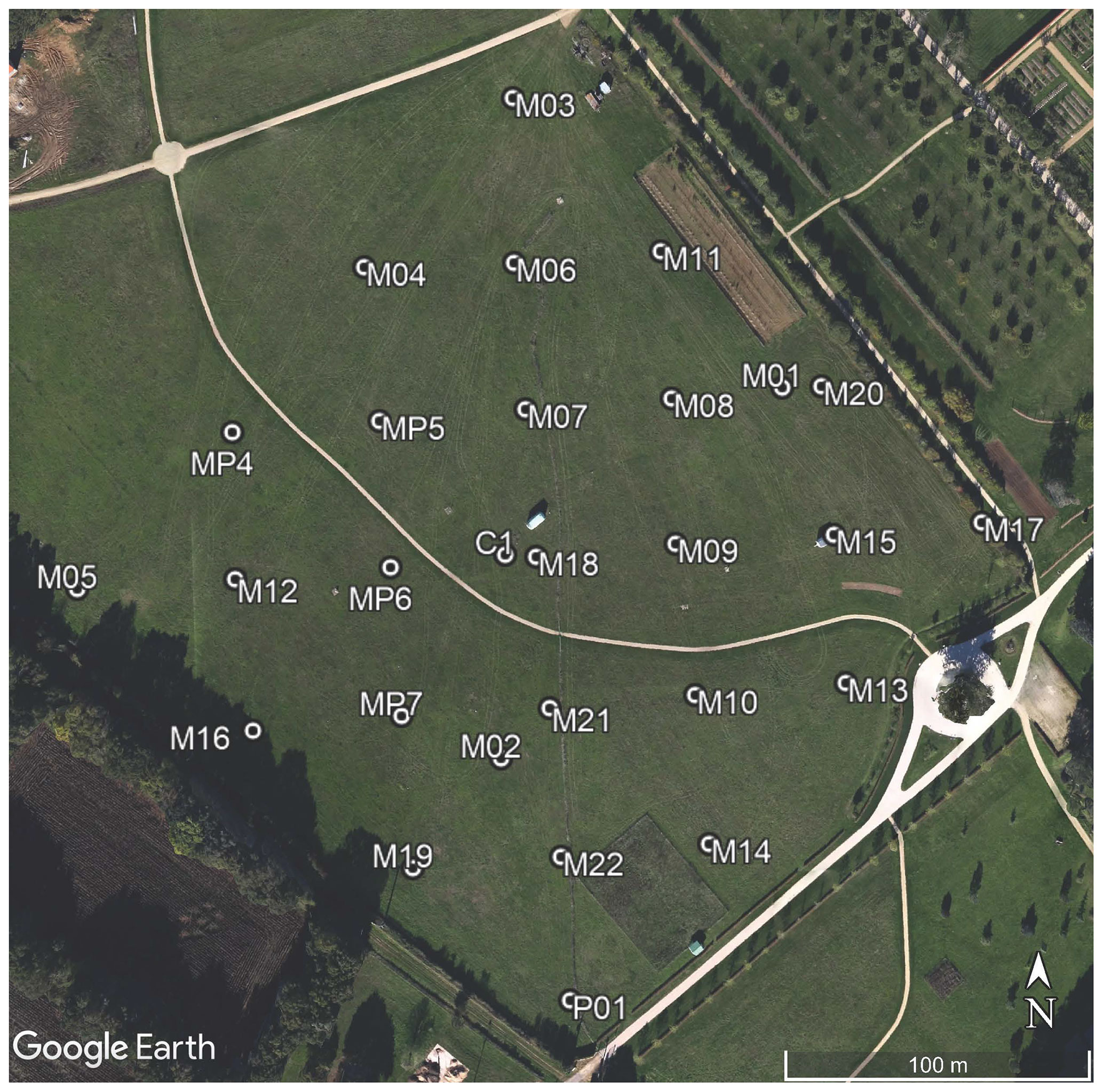
Figure 3 Location of the boreholes at the HES in Poitiers, France. Map data retrieved from © Google.

The bedded structure of the karst conduits is supported by observations of rock outcrops located a few km from the HES in the same lithostratigraphic horizons (Fig. 4). It is difficult to state whether the karst conduits present in a given horizon are all interconnected or whether they form different disconnected clusters. Similarly, it is difficult to determine whether natural high-permeability connections occur between the different karst layers, for example, through vertical fractures. However, there is evidence that certain boreholes provide connections by intersecting karst conduits in the different horizons. Even in the absence of pumping, vertical flows can be measured in these boreholes at velocities of up to several meters per minute, thus indicating a natural difference in hydraulic head between the various karst horizons.

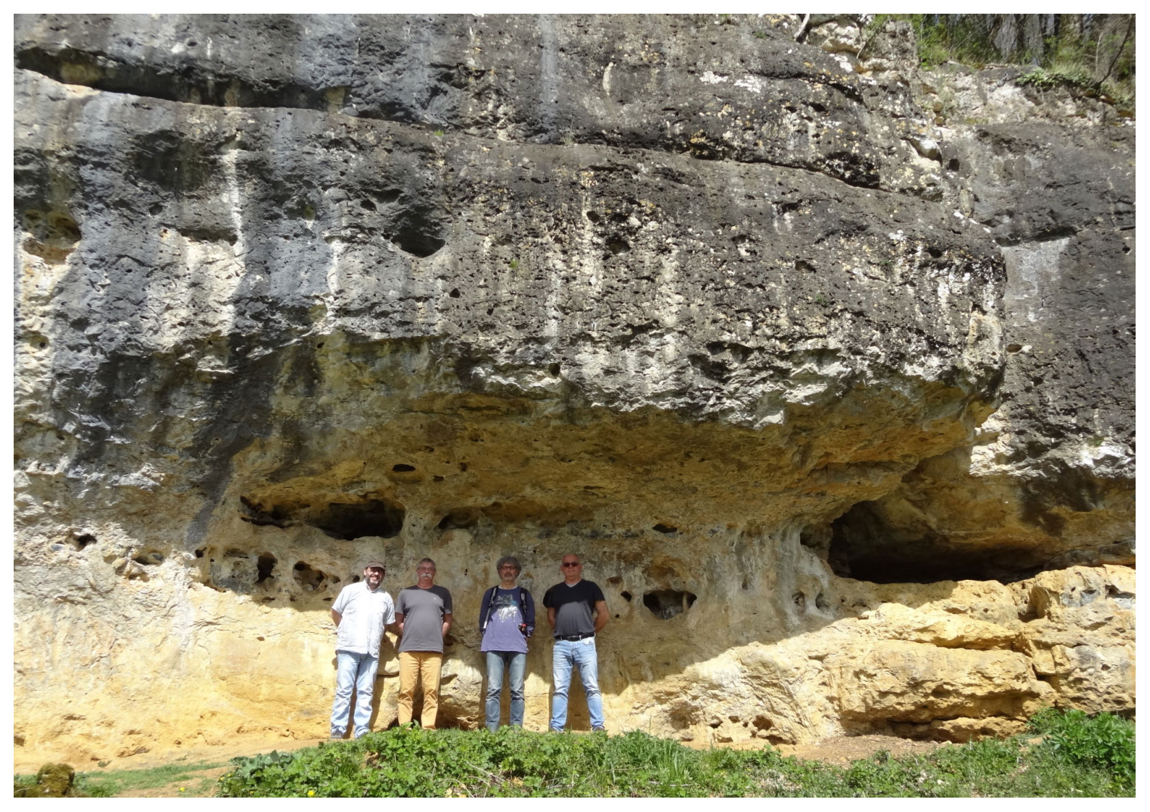
Figure 4 Bedded structure of karst conduits as observed on a rock outcrop located 5 km south of the HES.

A number of interwell tracer tests have been carried out at the HES over the last 5 years. The routine protocol applied in these tests can be summarized as follows:

1. A pumping operation is initiated at a constant rate ranging from 50–65 m³ h⁻¹, and a pseudosteady-state flow regime is eventually established, i.e., stabilization of the hydraulic head gradient over the HES area. The typical time for this regime to be reached is approximately 6 h, but usually a minimum of 24 h is observed before moving on to the next step.

2. Borehole flowmeter surveys are performed in the candidate wells for tracer injection: vertical flow velocities are measured, and possible inflow and outflow horizons are identified (Fig. 5).

3. The well and injection depth of the tracer are selected. The targeted injection depth is generally a few tens of cm upstream of an outflow (from the well to the aquifer) horizon. For instance, Fig. 5 indicates that a suitable injection depth for a tracer experiment between M02 and MP6 would be between 58 and 60 m depth.

4. Pipes 2.5 m in length and 1.5 cm in internal diameter are connected down to the targeted injection depth. This pipeline ends with a screened cap that ensures horizontal diffusion of the tracer at the outlet.

5. The tracer solution (typically 5 g of uranine diluted in 2 L of water) is injected, followed by a water flush volume of 40 L. The total injection duration, including flushing, is always less than 3 min.

6. The concentration at the outlet of the pumped well is monitored with a flow-through fluorometer (Albillia GGUN) connected to a bypass of the discharge pipeline.

The BTC dataset adopted in the present study corresponds to 50 tracer tests conducted between wells located in the area covered by seismic surveys. Four pumping wells were employed in the tracer experiments: M06, M07, M22, and MP6. Each BTC was processed with MFIT using both the multiflow ADE and 2RNE transport models. The multiflow SFDM was not adopted here because the typical duration of the considered tracer experiments, from a few hours to a few days, was insufficient for diffusion processes to be of influence. Actually, more precisely, this model could be fitted to the obtained HES tracer BTCs but without a better performance than that of the multiflow ADE model, which is simpler, or only if unrealistic diffusion parameter values were considered, e.g., Bodin (2020a). The optimal (minimum) number of channels N^* required to fit the above BTCs with the multiflow ADE and 2RNE models was determined as described in Sect. 2. The results are summarized as box plots in Fig. 6. The median N^* values obtained with the multiflow ADE and 2RNE models are 5 and 3, respectively. Rather than considering any form of competition between these two models, which are based on two different conceptual and mathematical approaches to the description of tracer migration in a heterogeneous medium, we instead believe that the N^* values associated with the multiflow ADE and 2RNE models allow us to differentiate between primary and secondary karst paths. The primary paths are those identified by the multiflow 2RNE model, while the secondary paths are the additional low-flow velocity channels explicitly required by the multiflow ADE model to fit the curves, where the multiflow 2RNE model simulates the exchange between the primary channels and surrounding stagnant water zones.

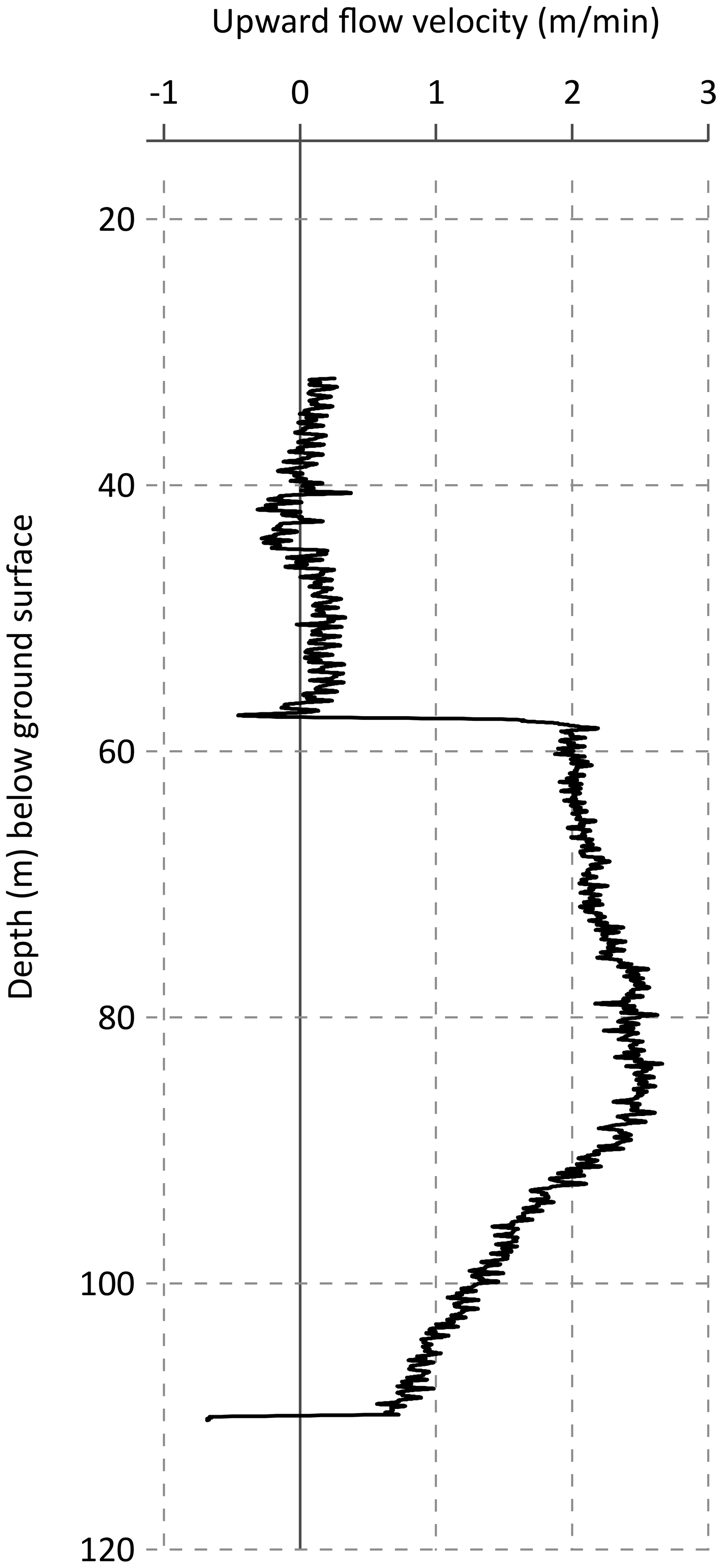
Figure 5 Example of borehole flowmeter data. The logged well is M02, while pumping is active in MP6 at a flow rate of 60 m³ h⁻¹. The flow velocity measurements indicate an upward flow from approximately 110 to 55 m below the ground surface. In this same pumping experiment, downward flows are measured in other boreholes. In this case, the curve is to the left of the vertical axis (negative upward flow velocity values).

A 3D seismic survey was conducted at the HES in 2004. The data were acquired along 21 parallel profiles running SW–NE and equidistant by 15 m. The SW–NE direction corresponds to a locally known structural (i.e., fracturation and karst) direction and is that of a small topographic valley in which boreholes M03, M04, MP4, and M05 were drilled. Each profile consisted of 48 geophones with an interdistance of 5 m. Five dynamite shots (25 g per shot) were fired for each line, one shot at each end and three perpendicular shots at 40, 50, and 60 m from the center of the line. In addition to the surface seismic surveys, full waveform acoustic logs were acquired in five boreholes (C01, MP5, MP6, M08, M09), and a vertical seismic profile (VSP) was acquired in C01. The procedure used to build the 3D seismic velocity model from the acquired data includes amplitude recovery, deconvolution, wave separation, normal move-out corrections, and time versus depth conversion based on VSP measurements. The acoustic logs in wells C01, MP5, MP6, M08, and M09 were used as calibration constraints for the seismic depth model. The interested reader can find further details in Mari and Porel (2008). The original seismic model grid consisted of 96 columns of 2.5 m in the SW–NE direction, 60 rows of 5 m in the NW–SE direction, and 512 layers of 0.5 m in the vertical direction from 0 to 256 m below the ground surface. In the present study, we truncated this model vertically by retaining only the 190 layers corresponding to the extension of the aquifer from 35 to 130 m below the ground surface (Fig. 7). As discussed by Mari and Porel (2008), the cross analysis of the 3D seismic model and the well logs shows a close relationship between low-seismic velocity zones and the main inflow and outflow horizons associated with high hydraulic conductivity features. The work presented below is based on the generalized assumption of a negative correlation between the seismic velocity and hydraulic conductivity.

Figure 6 Minimum number N^* of flow paths between the tracer injection and pumping well pairs identified with the multiflow 2RNE model and multiflow ADE model.

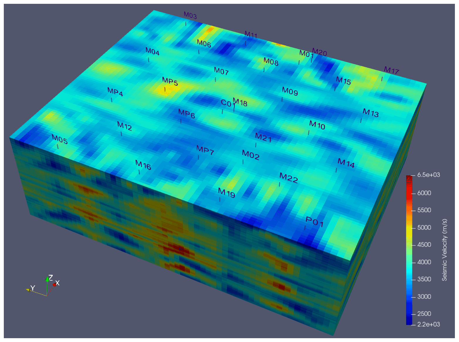
Figure 7 Three-dimensional seismic velocity model of the HES aquifer from 35 to 130 m below the ground surface.

The graph structure applied in pathfinding was acquired with (i) the 3D seismic velocity model and (ii) the borehole vertical flow velocity profiles measured prior to the tracer experiments. The Boost Graph Library (Siek et al., 2001) was adopted to generate a bidirectional graph whose vertices were mapped onto the centers of subseismic model grid cells. The vertices were connected with the 26-neighborhood rule. Each pair of neighboring vertices was connected by two edges, one in each direction. This option is primarily useful for the implementation of borehole flow patterns, as discussed below. In regard to all vertex pairs located between the boreholes and/or corresponding to borehole sections without major vertical flow, the two connecting edges were assigned identical weights. The weights were calculated as the arithmetic mean of the seismic velocity values multiplied by the Euclidean distance between the two vertices. This second factor corrected for the nonuniformity of the seismic model grid in all three spatial directions. In regard to the other edges, i.e., those corresponding to borehole sections where vertical flows were identified, the weights were calculated in two steps. First, the method described above was adopted, and a correction factor was then applied to promote any edges oriented along the flow direction and conversely penalize edges in the reverse direction. Since the vertical flow patterns and velocities in boreholes are basically dependent on the active pumping well, different edge-weight corrections were applied to the graph prior to searching for the optimal paths to wells M06, M07, M22, and MP6. The maximum velocity measured during the borehole flowmeter surveys was 3.5 m min⁻¹. Edge-weight corrections were applied to any borehole sections with a flow velocity higher than 0.1 m min⁻¹. The (multiplication and division) correction factor was empirically set to 15 times the velocity in m/min. This correction was also applied to the pumped well considering a vertical flow velocity calculated based on the pumping flow rate divided by the borehole cross section. The implemented graph structure comprised 1 094 400 vertices and 15 039 782 edges.

The conduit network obtained with the ARLib OnePass+ algorithm (please refer to Sect. 3) is shown in Fig. 8. As is the rule when modeling real groundwater systems, the results obtained cannot be validated but can only (eventually) be invalidated (Konikow and Bredehoeft, 1992). More specifically, strict validation would require new boreholes to be drilled to verify if they actually intersect the identified conduits. This operation is not envisaged at the HES, both because of its financial cost and because the creation of new boreholes could modify the flow-path structure by creating new bypasses between the different karst horizons.

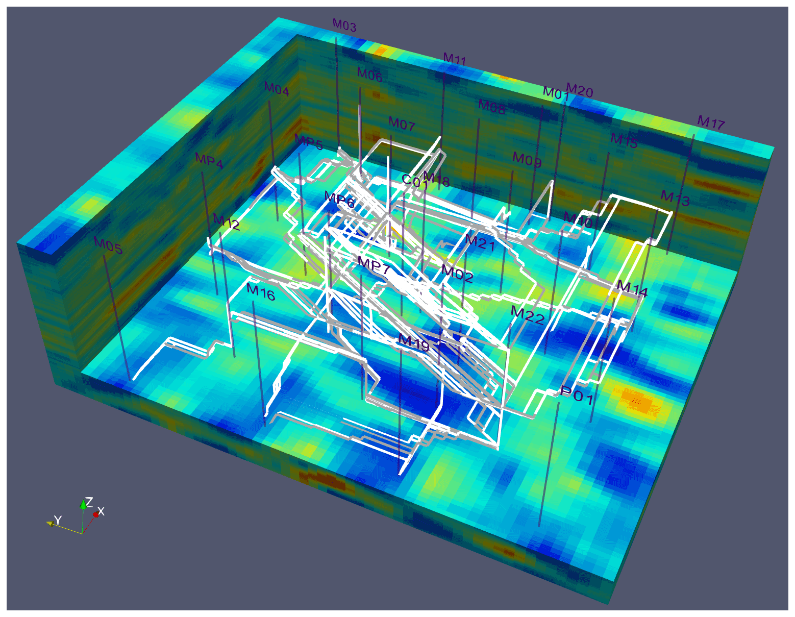
Figure 8 HES karst conduit network obtained from the combined analysis of interwell tracer tests, borehole flowmeter logs, and 3D seismic imaging data. The white and gray lines represent the main and secondary paths, respectively. The main paths are those identified via multiflow 2RNE inversion of the tracer BTCs, and the secondary paths are the additional paths identified via multiflow ADE inversion; please refer to Fig. 6.

Of the independent data against which the results can be confronted, it can be noted that (i) the computed network shows a layered structure that is consistent with the known karst horizons at 50, 90, and 115 m depth, and (ii) the statistical directional analysis of the conduits is also consistent with the local structural directions (Fig. 9). The N130–140 direction is not locally expressed on this outcrop, but it is a well-known regional karst direction, e.g., Bodin and Razack (1997). Conversely, the N–S and N110–120 fracture directions not found in the karst conduit inversion should not be considered to be of concern as it is well known that karst exploits only part of the original rock discontinuities (Bodin and Razack, 1997; Häuselmann et al., 1999).

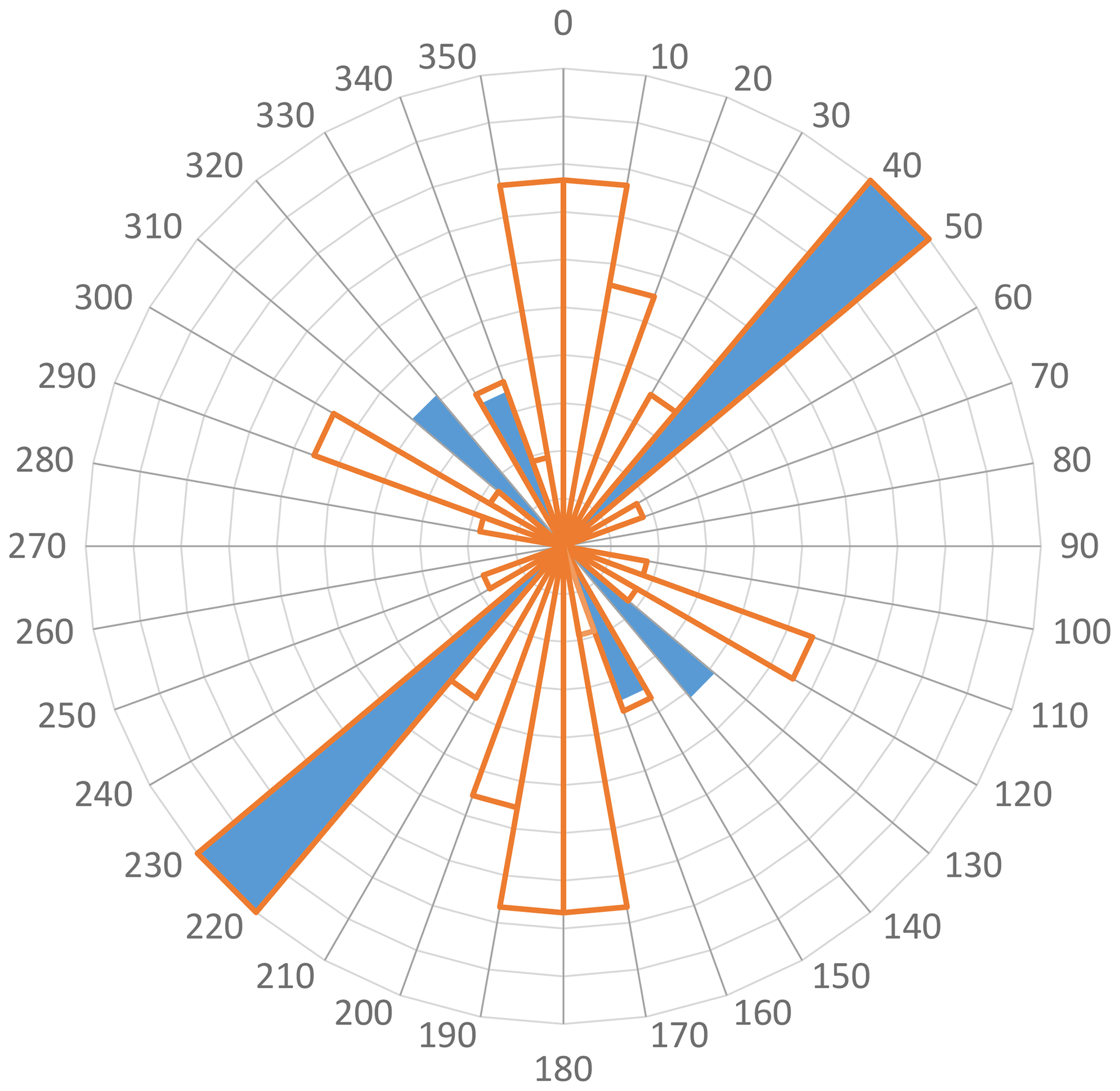
Figure 9 Normalized rose diagram of computed conduits (solid sectors) and measured fractures on a rock outcrop located 4 km west of the HES (empty sectors).

A very partial but direct verification of the computed network is also possible where the paths follow the vertical portions of boreholes. In the network, three boreholes likely play a vertical relay role between the different subhorizontal karst horizons: borehole MP7 between well M12 and pumped well M22, borehole M12 between M05 and MP6, and borehole M02 between M19 and MP6. As a pump was still present in MP6 when the network computation was completed, tracing experiments from M05 and M19 were again performed but with complementary concentration monitoring in intermediate boreholes M12 and M02 by means of fluorometers installed at depth. Other fluorometers were also installed at depth in nearby boreholes not expected to be in the tracer path. In terms of tracer experiment M05–MP6, the concentrations were monitored in MP4, M16, MP6, and M12. In terms of tracer experiment M19–MP6, boreholes MP7, M16, and M21 were monitored in addition to boreholes MP6 and M02. The results obtained, as shown in Fig. 10, are mostly as expected since the tracer actually flowed through intermediate boreholes M12 and M02 and was not detected in boreholes M16, MP4, and MP7. The only surprise was the observed unforeseen vertical transfer of the tracer through M21. These experimental results support the overall reliability of the calculated network but also expose its incompleteness. To test whether this incompleteness could occur due to the settings of the ARLib OnePass+ algorithm, the paths between M19 and MP6 were recalculated by lowering the value of parameter θ from 0.5 to 0.05 to increase interpath diversification. No path passing through M21 was identified. It is therefore likely that the incompleteness (or partial incorrectness) of the conduit network is primarily due to the resolution limits of the seismic data.

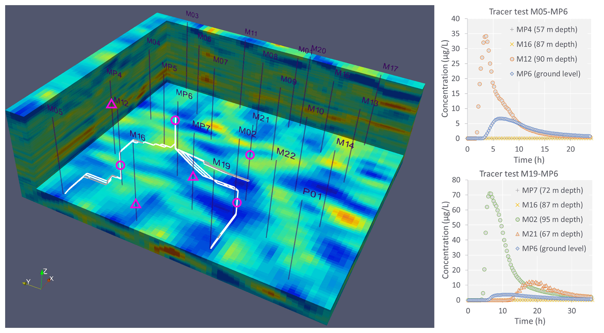
Figure 10 Verification tracer tests conducted between wells M05 (tracer injected at a 111 m depth), M19 (tracer injected at a 111 m depth), and MP6 (pumping well). The circles and triangles indicate the location of the fluorometer probes (Albillia GGUN FL22) that were or were not in the tracer path, respectively. The paths shown are those that have potentially been used by the tracer. The results obtained thus partially validate the paths M05–M12–MP6 and M19–M02–MP6. The main unknown is the connection between M19 and M21, especially as the vertical flow in M21 is downward.

5 Discussion and conclusions

The approach outlined in this paper aims to improve the assessment of conduit network geometry in karst aquifers. The prerequisite data for the application of the method are (i) a set of BTCs corresponding to tracer experiments conducted between different points in the karst network whose geometry is to be specified, and (ii) a 3D model of subsurface heterogeneity derived from geophysical methods sensitive to karst features. As discussed in the review of Chalikakis et al. (2011), most geophysical investigation methods are to a certain extent sensitive to karst features because the physical properties of a karst conduit filled with water are generally different from those of the surrounding rock. However, the downside is that the amplitude of the anomalies associated with karst conduits is often small, which results in an insufficient resolving capacity of geophysical methods to capture the geometry of karst networks unambiguously and accurately. The main strength of the approach we propose is to supplement the information content of geophysical surveys with the results of tracer BTC analysis. Part of the ambiguity in the identification of karst conduits based on geophysical data can be alleviated by building on the prior estimation of the number of conduits between pairs of point locations. The first step of the method is therefore to analyze each BTC using a regularized multiflow inversion method, as implemented in the MFIT software, to determine the minimum number of distinct paths used by the tracer between injection and monitoring points. The second step consists of implementing a graph based on the 3D geophysical model of subsurface heterogeneity and calculating the previously enumerated paths via the application of an alternative SP algorithm.

With the use of HES tracer test data, 3D seismic data, and borehole flowmeter logs to illustrate our approach, we have demonstrated the feasibility of delineating discrete karst conduit networks. The reliability of the identified network was locally verified through new tracer experiments performed after completion of the computations. To our knowledge, the present paper is the first to combine tracer and geophysical data to identify the discrete geometry of a karst network. Another conceivable approach would be the joint inversion of both types of data, but inversion methods based on a discrete approach to flow and/or transport paths are still at an early stage of development (e.g., Somogyvári et al., 2017; Fischer et al., 2020).

The main limitations of the proposed approach are (i) the spatial density of the tracer tests required to constrain the number of paths between the nodes of the network, and (ii) the sensitivity and/or spatial resolution problems inherent to geophysical methods. The M19–M21–MP6 pathway not identified from the HES data but highlighted a posteriori during the verification tracer tests is a concrete illustration of the limitations of the method. It must also be acknowledged that this approach allows the determination of only the backbone structure of the network and not the complete geometry of the karst conduit system, including the cross-sectional dimension and shape of conduits. Nevertheless, the implemented approach achieves substantial progress toward the characterization and subsequent modeling of karst aquifers. To complement the transport parameters of the individual karst conduits already inverted with MFIT, the computed network may be readily incorporated into hybrid discrete conduit-continuum models such as MODFLOW-USG (Panday et al., 2013) to calibrate the hydraulic parameters of the determined karst conduits and surrounding rock matrix against pumping test data. Finally, the approach may also be applicable to other types of aquifers in the delineation of preferential flow paths induced by subsurface heterogeneity provided that geophysical methods are sensitive to this heterogeneity.