the Creative Commons Attribution 4.0 License.
the Creative Commons Attribution 4.0 License.
 | 23 Mar 2022
Towards hybrid modeling of the global hydrological cycle
Martin Jung
Marco Körner
Sujan Koirala
Markus Reichstein
State-of-the-art global hydrological models (GHMs) exhibit large uncertainties in hydrological simulations due to the complexity, diversity, and heterogeneity of the land surface and subsurface processes, as well as the scale dependency of these processes and associated parameters. Recent progress in machine learning, fueled by relevant Earth observation data streams, may help overcome these challenges. But machine learning methods are not bound by physical laws, and their interpretability is limited by design.
In this study, we exemplify a hybrid approach to global hydrological modeling that exploits the data adaptivity of neural networks for representing uncertain processes within a model structure based on physical principles (e.g., mass conservation) that form the basis of GHMs. This combination of machine learning and physical knowledge can potentially lead to data-driven, yet physically consistent and partially interpretable hybrid models.
The hybrid hydrological model (H2M), extended from Kraft et al. (2020), simulates the dynamics of snow, soil moisture, and groundwater storage globally at 1∘ spatial resolution and daily time step. Water fluxes are simulated by an embedded recurrent neural network. We trained the model simultaneously against observational products of terrestrial water storage variations (TWS), grid cell runoff (Q), evapotranspiration (ET), and snow water equivalent (SWE) with a multi-task learning approach.
We find that the H2M is capable of reproducing key patterns of global water cycle components, with model performances being at least on par with four state-of-the-art GHMs which provide a necessary benchmark for H2M. The neural-network-learned hydrological responses of evapotranspiration and grid cell runoff to antecedent soil moisture states are qualitatively consistent with our understanding and theory. The simulated contributions of groundwater, soil moisture, and snowpack variability to TWS variations are plausible and within the ranges of traditional GHMs. H2M identifies a somewhat stronger role of soil moisture for TWS variations in transitional and tropical regions compared to GHMs.
With the findings and analysis, we conclude that H2M provides a new data-driven perspective on modeling the global hydrological cycle and physical responses with machine-learned parameters that is consistent with and complementary to existing global modeling frameworks. The hybrid modeling approaches have a large potential to better leverage ever-increasing Earth observation data streams to advance our understandings of the Earth system and capabilities to monitor and model it.
- Article
(16070 KB) - Full-text XML
- BibTeX
- EndNote


Physically based global hydrological models (GHMs) are an essential tool to understand, monitor, and forecast the water cycle, with an array of societal implications (Jiménez Cisneros et al., 2014). Yet, GHMs and land surface models face many challenges related to process representations and parameterizations, resulting in large uncertainties (Schellekens et al., 2017). The existing state-of-the-art GHMs still disagree across all spatial and temporal scales, which may be attributed to limited, biased, and uncertain data, the heterogeneity of considered processes, or a lack of process understanding (Haddeland et al., 2011; Beck et al., 2017). While global water cycle observations are increasing rapidly, a thorough integration with a GHM to overcome uncertainties is rarely facilitated due to the model complexity and computational expenses, even though some GHMs use data, e.g., river discharge, to calibrate model parameters (e.g., Van Beek et al., 2011).
Different pathways have been proposed to utilize additional Earth observation data in hydrological modeling. For instance, physically based models benefit from using spatially explicit parameters, which can be retrieved from Earth observation data. It is, for example, common to use spatiotemporally varying leaf area index as a model parameter (e.g., Van Der Knijff et al., 2010) to account for vegetation dynamics. Furthermore, upscaling of locally estimated or measured parameters to global scale – such as catchment parameters (Beck et al., 2016) or soil properties (Hengl et al., 2017) – can improve model accuracy. Using model–data integration approaches, it has been shown that relatively simple conceptual hydrological models can yield state-of-the-art performance when calibrated simultaneously on multiple observational data constraints (Trautmann et al., 2018), which opens new avenues for targeted, partially data-driven experiments to parameterize hydrological processes.
Other approaches to integrate additional observations and physically based models have been developed in the domain of data assimilation (McLaughlin, 2002; Reichle, 2008). While classic data assimilation aims to correct model states or provide initial conditions using additional observational data (Sun et al., 2016), promising concepts exist to learn time-varying model parameters from data (Moradkhani et al., 2005; Geer, 2021). If system understanding and out-of-sample performance (e.g., long-term prediction) are not central, then the use of (purely data-driven) deep learning approaches has been proposed and applied recently in hydrology, and experimental methods for gaining (so far only qualitative) insights exist (Shen et al., 2018).
Recently, it has been proposed to fuse process models with machine learning into one end-to-end modeling system in the so-called hybrid modeling approaches (Reichstein et al., 2019). The hybrid approaches aim at harvesting the information in Earth observation data efficiently by replacing uncertain parameters and processes with a machine learning model, while still maintaining model interpretability and physical consistency. Furthermore, the approach facilitates the incorporation and integration of information from multiple data sources, which is a bottleneck in GHMs. Hybrid modeling can be employed to improve the predictability of the Earth system or components thereof, such as sea surface temperature (de Bézenac et al., 2019) or subgrid atmospheric processes (Rasp et al., 2018). Alternatively, but not mutually exclusive, hybrid modeling can leverage the flexibility of machine learning models with the goal to retrieve data-driven, yet interpretable, physical coefficients and latent variables.
One of the key hydrological data products for diagnosing and understanding global land water cycle variations is total terrestrial water storage (TWS). The TWS is an observation-based rasterized product that integrates all water storage components and is used for calibration and validation of process-based models (Güntner et al., 2007; Schellekens et al., 2017; Trautmann et al., 2018; Scanlon et al., 2019) and in data-driven studies (Humphrey et al., 2016; Andrew et al., 2017; Rodell et al., 2018). An attribution of TWS variations to its components is still unclear, as current model simulations do not produce consistent spatiotemporal patterns due to uncertainties in the model structure and process description, forcing data, and parameter values (Güntner, 2008). Such attribution is not trivial, especially as contiguous observations of the storage components are not available separately on a global scale (e.g., groundwater) or limited (e.g., soil moisture, where satellite observations are only representative of the top soil layers). Thus, decomposition of TWS components is either done with large-scale hydrological modeling (Schellekens et al., 2017), locally using in situ data (e.g., Swenson et al., 2008), or with data-driven approaches without a strict constraint on physical consistency (Andrew et al., 2017).
This study aims to complement and bridge the previous global-scale hydrological modeling and observation-based syntheses by comprehensively evaluating the potential of hybrid modeling at the global scale. In particular, it provides a much-needed data-driven perspective on the global water cycle and its spatiotemporal variability based on carefully designed cross-validation analysis, together with a crucial consideration of the basic physical principle of mass conservation. To do so, we have further developed the model proposed by Kraft et al. (2020), especially with regards to model robustness and physical consistency. The overarching goal of this study is to provide a comprehensive description and assessment of the applicability of the hybrid modeling approach as a potential novel avenue for global hydrological simulation. Particular emphasis are put on benchmarking against and complementing state-of-the-art hydrological models and assessing the plausibility and interpretability of the machine-learning-based data-driven hydrological responses going beyond the typical focus on predictive skills. Furthermore, we examine the potential applications and limitations on a challenging use case of decomposing the contributions of different water storage components to the variations of TWS.
We first describe the datasets used, the hybrid hydrological model (H2M), and the model training and evaluation approach in Sect. 2. We then show the H2M performance in Sect. 3.1 and present the benchmarking against a set of GHM simulations from the eartH2Observe ensemble in Sect. 3.2. Section 3.3 provides the data-driven perspective on hydrological responses, followed by Sect. 3.4, which focuses on the TWS decomposition. Additional plausibility and interpretability of the H2M simulations are presented in Sects. 4.1 and 4.2. Last, we provide a more general assessment of the challenges and opportunities of the hybrid approach in Sect. 4.3.
2.1 Datasets
2.1.1 Meteorological forcing
A total of three time-varying meteorological datasets were used to force H2M as follows (Table 1):
- i.
Precipitation observations, obtained from the Global Precipitation Climatology Project dataset (GPCP-1DD) v1.2 (Huffman et al., 2012),
- ii.
Net radiation, provided by the SYN1deg Ed3A product (Doelling, 2017) of the Clouds and the Earth's Radiant Energy Systems (CERES) program (Wielicki et al., 1996), and
- iii.
Air temperature, obtained from CRUNCEP v8 dataset, a product of the observation-based Climatic Research Unit (CRU) and the National Centers for Environmental Prediction (NCEP) reanalysis data (Harris et al., 2014; Viovy, 2018).
Table 1Dataset overview, including water cycle constraints, meteorological forcing, and static variables with their native and aggregated spatial and temporal resolution. We use upper case for state variables and lower case for fluxes in the mathematical notation.
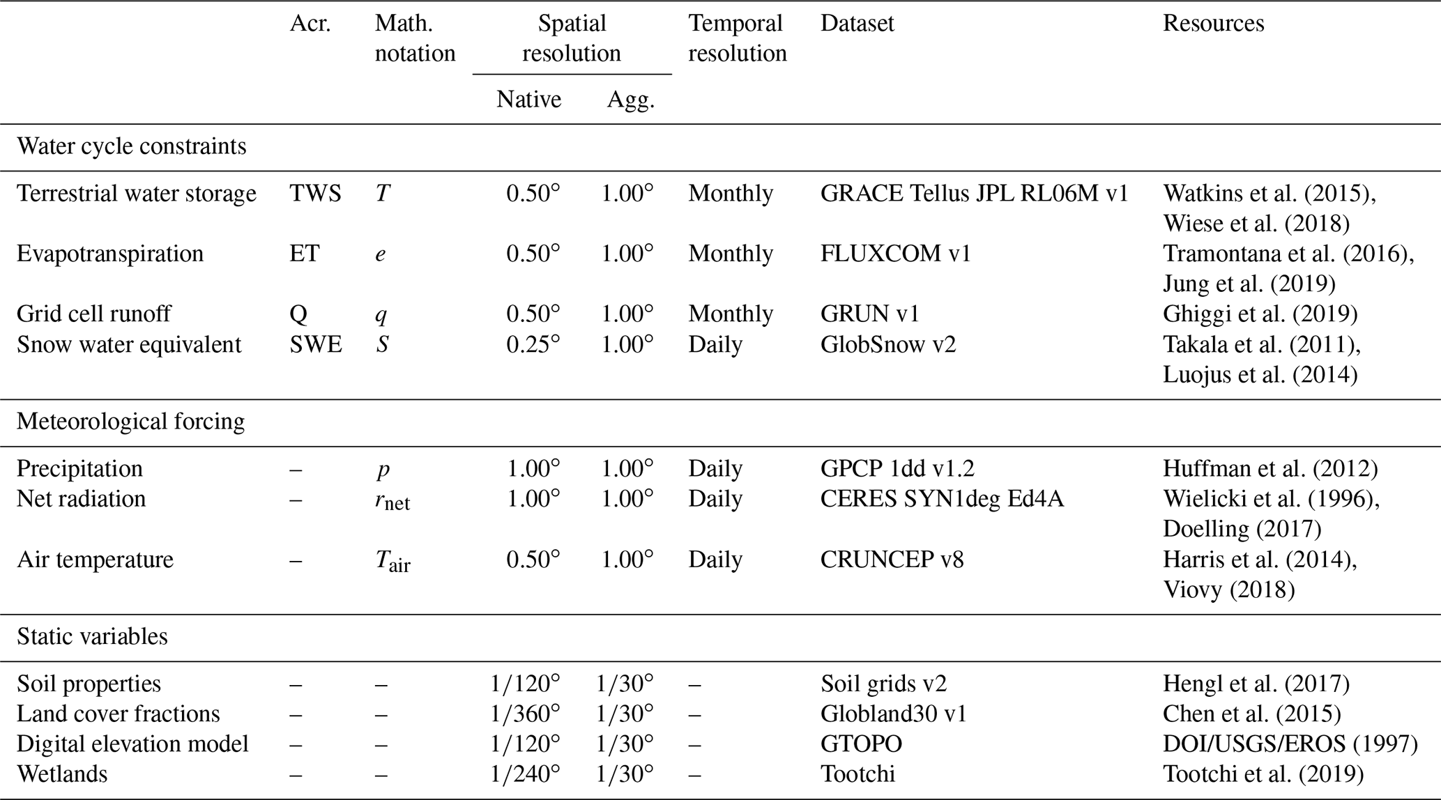
Note: Acr. – acronym; Agg. – aggregated.
To test the impact of the model forcings on the comparison with GHMs (Sect. 3.2), we carried out additional H2M simulation with forcing datasets from the WATCH Forcing Data–ERA-Interim (WFDEI) dataset (Weedon et al., 2014) in an independent setup (Appendix D).
2.1.2 Static variables
A set of temporally static variables was used to represent land surface characteristics as follows (Table 1):
- i.
The soil properties from the SoilGrids dataset (Hengl et al., 2017), including absolute depth to bedrock and the average (along depth) of the bulk density, coarse fragments, clay, silt, and sand (six variables in total).
- ii.
The land cover fractions from the GlobeLand30 dataset (Chen et al., 2015) for the 10 classes of water bodies, wetlands, artificial surfaces, tundra, permanent snow and ice, grasslands, barren, cultivated land, shrublands, and forests.
- iii.
The digital elevation model from GTOPO30 (DOI/USGS/EROS, 1997).
- iv.
The fractions of groundwater-driven wetlands, regularly flooded wetlands, and the intersection of them (Tootchi et al., 2019), i.e., a total of three variables.
These 20 static variables were spatially aggregated from their finer resolution to ∘ to maintain sub-grid variations, yielding a block of 30 latitude cells times 30 longitude cells times 20 variables, i.e., a total of 18 000 values per 1∘ grid cell, which is the spatial resolution of the forcing data. Due to the high dimensionality of the static variables, the data were compressed in a preprocessing step using a simple convolutional auto-encoder, consisting of an encoder, a bottleneck layer, and a decoder. The encoder is a stack of consecutively smaller convolutional neural network (CNN) layers that reduce the input block to a vector of size 30, i.e., the bottleneck layer. This process is then reverted in the decoder model, mapping the vector back to the input data. The CNN model is optimized to reconstruct the input data but is forced to find a low-dimensional representation enforced by the bottleneck (e.g., Goodfellow et al., 2016). The resulting compressed dataset consists of 30 latent variables per grid cell that encode the original high-dimensional data (18 000), which is then used as an input to H2M (Sect. 2.2.2). Note that this preprocessing step was done independently from the training of H2M.
2.1.3 Observational constraints
In total, four observational hydrological variables were used to constrain H2M. The datasets were aggregated to a common spatial resolution of 1∘ (Table 1). Due to differences in temporal coverage of the data products, a common period of February 2002 to December 2014 was selected.
- i.
The monthly TWS observations from the Gravity Recovery and Climate Experiment (GRACE) Mascon Equivalent Water Height RL06 with Coastal Resolution Improvement (CRI) v1 (Watkins et al., 2015; Wiese et al., 2016, 2018) reflect vertically integrated variations in the water storage. These include the total variations in all storage components, including groundwater, soil moisture, surface water, biosphere-bound water, snow, and ice. To minimize the effect of outliers on the H2M performance, the TWS observations outside the range of −500 to 500 mm were excluded.
- ii.
Monthly ET estimates were obtained from the global FLUXCOM-RS product (Tramontana et al., 2016; Jung et al., 2019), which is based on machine-learning-driven estimates that are upscaled from site-level FLUXNET eddy covariance measurements (Baldocchi et al., 2001) to a global scale using a range of satellite-based drivers. ET was converted from latent energy estimates assuming a constant latent heat of vaporization of 2.45 .
- iii.
Monthly Q estimates were obtained from the GRUN v1 dataset (Ghiggi et al., 2019). GRUN is based on an upscaling approach that correlates small catchment observations of Q to climate variability. The machine-learned relationships are then generalized to the global scale. Note that only catchments with an area similar to the spatial resolution of the meteorological forcings were used for the prediction, and thus, Q does not include larger routed streamflows and provides an estimate of gridded runoff.
- iv.
The daily SWE observations were obtained from the GlobSnow v2 product (Takala et al., 2011; Luojus et al., 2014). GlobSnow provides snow water equivalent in the Northern Hemisphere above 40∘ N, while the mostly snow-free Southern Hemisphere is not covered. In GlobSnow, the time steps with no snow are encoded as missing values. Thus, we gap-filled the GlobSnow product but only with zero values if (a) the snow cover fraction from MODIS (Hall and Riggs, 2016) was below 10 % and (b) the GlobSnow product had missing values in a window of ±12 d. The remaining missing values were not altered.
2.1.4 Global hydrological model ensemble
To evaluate the H2M simulations of TWS and its components, we selected the GHMs from the eartH2Observe ensemble (Schellekens et al., 2017) version WWR1. From the 10 available model simulations, we selected the ones which included groundwater storage: LISFLOOD (Van Der Knijff et al., 2010), W3RA (Van Dijk and Warren, 2010; Van Dijk et al., 2014), PCR-GLOBWB (Van Beek et al., 2011; Wada et al., 2014), and SURFEX-TRIP (Decharme et al., 2010, 2013).
As the models represent different water storages (Table 2), they were combined to conceptually match storages modeled in the H2M (see Sect. 2.2.1). Snow water equivalent (SWE) is available in all models and was used as is. Groundwater (GW) storage, conceptualized as all delayed storage components, is the sum of groundwater and surface storage (SStor), if available for a model. Soil moisture (SM) was combined with canopy interception (CInt), if available. Note that the H2M does not represent SM directly but the cumulative soil water deficit (CWD), but we consider the dynamics of negative CWD to correspond to SM, and thus, the terms are used interchangeably when talking about soil moisture dynamics.
Table 2The terrestrial water storage (TWS) components as represented by the selected process models. While the hybrid hydrological model (H2M) represents snow water equivalent (SWE) explicitly, like the process models, the remaining TWS components are partitioned into soil cumulative water deficit (CWD) and groundwater (GW), which can be interpreted as fast and slow storage. To compare these components to the global hydrological models (GHMs), we calculated the storage as soil moisture plus canopy interception (CInt) if available and groundwater plus surface storage (SStor) if available, respectively. Note that CWD represents a deficit and, thus, it corresponds to negative soil water storage.

Note: SWE – soil water equivalent; CWD – cumulative soil water deficit; GW – groundwater; SM – soil moisture; CInt – canopy interception; SStor – surface storage.
The GHMs were aggregated spatially from 0.5∘ to match the 1.0∘ resolution of our simulations. Such spatial aggregations for model comparison are common practice in model intercomparison studies (e.g., Taylor et al., 2012). We expect the variations within four 0.5∘ cells to be small and thus assume that the 1.0∘ aggregation does not distort the modeled large-scale spatial patterns.
2.1.5 Data filtering
The data used for H2M were additionally filtered to remove regions with low variations in the hydrological cycle, high anthropogenic impact, and with known data limitations, using the following criteria:
-
grid cells with more than 50 % water bodies, more than 90 % permanent snow or ice, or more than 90 % bare land,
-
regions with more than 90 % artificial built-up surfaces,
-
regions with large groundwater withdrawals labeled as groundwater depletion under anthropogenic influence in Rodell et al. (2018),
-
grid cells with more than 50 % missing values in any of the time series of the observational constraints, and
-
mountainous areas, which are masked in GlobSnow.
After applying the filters, a total of 12 084 of 1∘ grid cells, covering roughly 80 % of the global land area, were selected.
2.2 The hybrid hydrological model (H2M)
The H2M consists of a dynamic neural network and a simple hydrological framework that represent the major water fluxes and changes in water storage (Fig. 1).
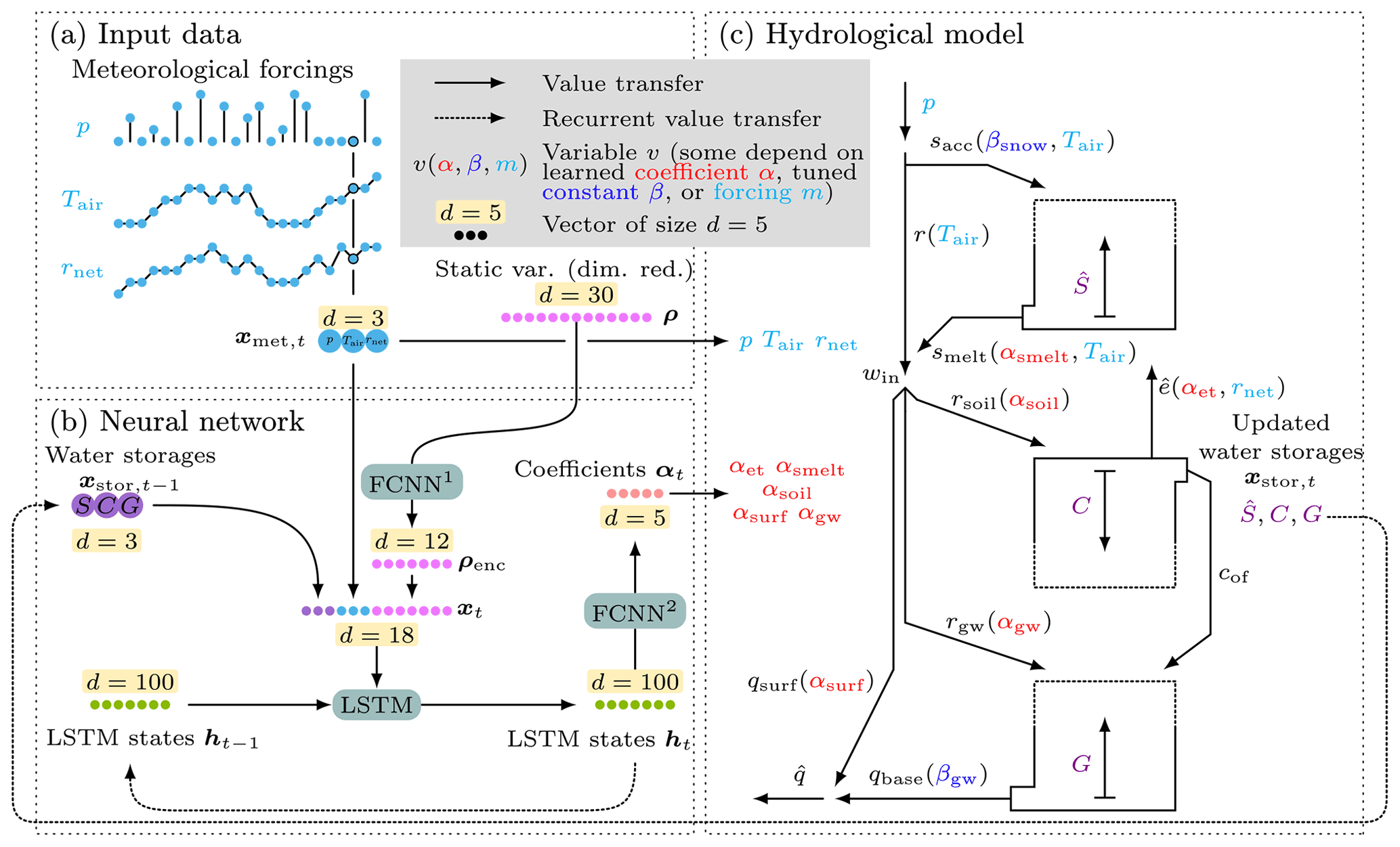
Figure 1In the H2M, a (b) dynamic neural network (NN) simulates a set of time-varying coefficients that are used in a simple (c) hydrological model. The meteorological forcings xmet,t at time t are used as input (a) to the NN and to the physical equations. The NN contains a long short-term memory (LSTM) layer and two fully connected networks (FCNNs). The model maintains two sets of states, namely the (physical) water storages xstor and the LSTM's internal (non-physical) state h (cell state omitted here). It is conditioned on additional inputs representing static land surface and soil properties ρ and the previous water storages . The NN module yields five time-varying coefficients (α) which are used in the balance equations. In total, two global parameters (β) are estimated independently from the data input directly by the optimizer. The location of usage in the balance equations is indicated in parentheses, () denotes the variables that are constrained with observations, and upper case variables are storages. Forcings (cyan): p – precipitation; Tair – air temperature; rnet – net radiation. Water storages (purple): – snow water equivalent; C – cumulative soil water deficit; G – groundwater. Time-varying coefficients (red): αsoil – soil recharge fraction; αgw – groundwater recharge fraction; αsurf – surface runoff fraction; αsmelt – snowmelt coefficient; αet – evaporative fraction. Learned global constants (blue): βsnow – snow undercatch correction constant; βgw: baseflow constant. Water fluxes: r – rainfall; sacc – snow accumulation; smelt – snowmelt; win – liquid phase water input; rsoil – soil recharge; rgw – groundwater recharge; – evapotranspiration; cof – overflow; qsurf – surface runoff; qbase – baseflow; – total runoff.
The H2M is set up as a global model, i.e., the same model is used to predict the full spatiotemporal domain, in contrast to separate models for each grid cell in a local setup. The H2M only considers the vertical flow/transport of the water through the system and does not include the lateral flow of either surface (river routing) or sub-surface water (groundwater flow).
The neural network (Sect. 2.2.2) yields a set of time-varying coefficients conditioned on the meteorological forcing and spatial properties derived from the static input variables. These coefficients (e.g., snowmelt factor) are then used in a set of hydrological equations that are introduced in Sect. 2.2.1. For inference (after the optimization of the neural network), the model can be applied to unseen data like any forward simulation model without further model tuning.
For the sake of consistency and clarity, α denotes the time-varying coefficients that are directly estimated by the neural network, and β denotes the global parameters that are learned as spatially constant. Throughout the paper, t is used as time index and i as the grid cell index. Uppercase variables are used for physical state variables. The code is available online (see the code and data availability section).
2.2.1 Hydrological components
In this section, we introduce the main hydrological components of the H2M.
Snow
Snow water equivalent is one of the water storages simulated by the H2M, and it is also constrained by the corresponding observation during model training.
Snow accumulation is precipitation p with air temperatures Tair≤0 ∘C, as follows:
The accumulation is scaled by a learned (optimized) global constant . The correction accounts for the known overestimation of solid precipitation due to over-correction for under catch of snowfall in gauge measurements (Decharme and Douville, 2006). Potential snowmelt is then calculated using a degree day approach, as follows:
Opposite to snow accumulation, smelt occurs under the condition of Tair>0 ∘C. The time-varying snowmelt coefficient αsmelt is estimated by the neural network module and mapped to positive values by applying the softplus activation function, i.e., . The snow water equivalent is then updated using snow accumulation and melt, as follows:
Positive values of S are enforced by truncating negative values.
The temperature constraints on snowmelt and accumulation were introduced to avoid compensation effects between sacc and smelt. It must be noted that such constraints are needed despite the fact that the relationship between snowfall or snowmelt and air temperature at 2 m may not always be realistic due to the corresponding associations with atmospheric (for snowfall) and land surface conditions (for snowmelt). We argue that the constraint will reduce or ideally remove equifinality among the parameters, and thus increase identifiability. This would allow for a physical interpretation of the parameters and processes.
Soil recharge, groundwater recharge, and surface runoff
The water input (in liquid form) win (mm d−1) is the sum of snowmelt and rainfall. It is partitioned into three fluxes, namely surface runoff, qsurf, soil recharge, rsoil, and groundwater recharge, rgw.
The coefficients for the partitioning are estimated by the neural network module and mapped to the range (0,1) and naturally constrained to the sum of 1 by applying the softmax transformation; for the element j of K elements. The softmax transformation generalizes the logistic function to multiple dimensions. Note that the constraint ensures that the incoming water is neither lost nor generated during the partitioning, respecting the physical law for the conservation of mass.
From the partitioning coefficients, soil recharge rsoil, groundwater recharge rgw, and surface runoff qsurf fluxes are then calculated as follows:
respectively, where αsoil, αgw, and αsurf are the partitioning coefficients of the total incoming water win. All partitioning parameters vary in both space and time.
Evapotranspiration and soil moisture
The total evapotranspiration is calculated as the product of the evaporative fraction αet and net radiation rnet () converted to mm d−1 assuming a latent heat of vaporization of 2.45 , as follows:
The evaporative fraction is learned by the neural network and mapped to the range (0,1) by applying the sigmoid activation function of . Note that evapotranspiration is constrained by the corresponding observation during model training.
Once the evapotranspiration and soil recharge are calculated, the soil moisture is parameterized as the cumulative soil water deficit C≥0 as follows:
which has the benefit of having a physical saturation limit of 0. For the comparison with the GHMs (Sect. 3.2), we calculate soil moisture (mm) dynamics as . The state C is updated by addition of the soil recharge rsoil, subtraction of evapotranspiration e (Eq. 8), and leveling by the overflow mechanism (Eqs. 9 and 10). If C approaches 0, an overflow mechanism allows for direct discharge of excess soil moisture into the deeper groundwater storage. Due to the heterogeneity within a model cell, the overflow cof starts already at values close to 0, which is achieved by using the softplus function.
Baseflow and groundwater
The baseflow is calculated as fraction of the past groundwater storage Gt−1 via the learned global baseflow constant βgw with the range (0,1), as follows:
Once the baseflow, groundwater recharge, and overflow of soil storage are calculated, the groundwater storage can be updated using a simple water balance, as follows:
In H2M, G represents an unconfined aquifer with an unlimited storage capacity.
Total runoff
The total runoff is simply calculated as the sum of the surface runoff qsurf (Eq. 6) and the baseflow qbase (Eq. 11), as follows:
We emphasize here that the neural network receives the state of water storage as inputs and is, thus, able to learn interactions of the water storages, the input variables, and the corresponding hydrological partitioning and outflow coefficients. Thus, the runoff generation and evapotranspiration processes do not only depend on the current and past meteorological condition and static variables but also on hydrological state, e.g., the soil water deficit. Therefore, we additionally use runoff as a data constraint during model training.
H2M storage components
For model training against GRACE, the variations in the modeled terrestrial water storage components are added to calculate the total terrestrial water storage as follows:
Note that −C is used in Eq. (14) as C itself is defined as the water deficit. As the observations of the terrestrial water storage from GRACE represent the temporal variations, the mean of simulated storage were removed from each grid cell as follows:
where k is the time step of 𝒯 total steps. The TWS is constrained by observations during model training.
Note that H2M does not represent surface water storage – a fourth major component of TWS, dominant especially in and around large surface water bodies like rivers and lakes – explicitly. This will be considered in the discussion of the results.
Compared to physically based models, the H2M does not explicitly partition the sub-surface storages as soil moisture and groundwater storages. Rather, it is represented as GW and CWD. The partition is an emergent behavior of H2M constraints by the major hydrological fluxes. Negative CWD is loosely and conceptually interpreted as root zone soil moisture, as it serves as the moisture source for evapotranspiration. This is in fact consistent with the physical models, even though CWD does not have a continuous interaction with GW storage except during overflow in H2M.
GW storage represents all delayed residual liquid water storage with infinite capacity. It is constrained by the baseflow fraction and subsequently temporal variation of total runoff (Eq. 11), which leads to a delayed dynamics compared to CWD.
2.2.2 The neural network (NN) module
The NN module (Fig. 1b) consists of three consecutively arranged sub-modules employed for extractions of different features. Overall, the NN module learns the spatiotemporally varying coefficients of the hydrological model using meteorological and dimensionality-reduced static variables of land (sub-)surface characteristics. The pseudocode of the NN module is presented in Appendix E, while the sub-modules are introduced here.
The first feed-forward (i.e., non-temporal) sub-module learns a compressed representation of the static variables (Eq. 16). This representation, together with meteorological input, is then fed into the second sub-module, a recursive long short-term memory (LSTM) model (Hochreiter and Schmidhuber, 1997), as shown in Eq. (17). The third sub-module (Eq. 18) transforms the outputs of the LSTM to a set of coefficients, which are then fed into the hydrological components. As the model weights are shared across all grid cells, the NN module learns from the global dynamics and not exclusively from each grid cell. For a comprehensive overview of the neural network architectures, see Goodfellow et al. (2016).
The first sub-module is a fully connected neural network (FCNN1 in Fig. 1), with a single hidden layer and 150 nodes, as follows:
It takes the static encodings ρ (see Sect. 2.1.2) as inputs and transforms them into a more condensed form (ρenc). This reduces the high dimensionality of static inputs from 30 to 12 values. Ideally, this lower-dimensional representation describes the most significant gradients of the land characteristics at the sub-grid scale (visualized in Fig. C2; Appendix C). Note that the static variables have already been compressed in a preprocessing step, and the transformation in this sub-module is optimized specifically for the parameterization of the hydrological components.
The second sub-module is an LSTM, a recurrent neural network (RNN) variant that updates its states dynamically using the previous states and the current input. LSTMs are broadly used in the Earth sciences due to their ability to learn temporal dynamics (Körner and Rußwurm, 2021), i.e., to represent memory effects that are present in hydrological observations (Kraft et al., 2019, 2021a; Humphrey et al., 2016). It has a hidden (in the sense of latent) state vector h whose length (100 in H2M) is a tunable hyperparameter. The hidden state is updated at each time step by using interactions of the previous states and the current input xt,i, as follows:
A further cell state c was omitted here for simplicity. In H2M, xt,i is a multivariate input consisting of concatenated current meteorological conditions , antecedent physical states from the hydrological model , and the static features ρenc,i from Eq. (16). The input allows the LSTM to learn interactions among the variables conditioned on static land properties like land cover type or elevation. In the optimization process, the RNN learns to maintain a memory of information from past time steps and is capable of updating, removing, and extracting information from its state.
In summary, the LSTM sub-module is similar to a physically based model – it takes the current inputs and static characteristics and updates the system state based on their interactions with the past state. It should be noted that neither its hidden state nor the update function is physically interpretable.
Last, the third sub-module linearly maps the LSTM output h to the coefficients α of the hydrological components (FCNN2 in Fig. 1), as follows:
The vector α contains five time-varying scalars corresponding to soil recharge fraction αsoil, groundwater recharge fraction αgw, surface runoff fraction αsurf, snowmelt coefficient αsmelt, and evaporative fraction αet.
2.3 Model training
This section introduces the necessary aspects of the model training and validation. First, we introduce the cross-validation setup, followed by the model training, and the loss function.
2.3.1 Cross-validation setup
We use k-fold cross-validation to validate the H2M against observations that were withheld during the training. In the cross-validation, the model is optimized first on a set of training grid cells and applied to a different set of test grid cells, i.e., spatial splitting. Specifically, the grid cells were first split into four sets of grids , each consisting of every second grid cell in latitude and longitude direction with an offset Ol. The offsets of are chosen such that the selected grids did not overlap while covering the full spatial domain. This procedure asserts a minimum distance needed to avoid potential issues of spatial autocorrelation (Roberts et al., 2017) within each grid. Each grid was then randomly subdivided into five folds for cross-validation, with three folds for training and one each for validation and testing. The validation subset was used in early stopping, i.e., to stop the training after the validation loss increases over several consecutive iterations. After the training stop, the best model parameters are loaded and predictions are made on the test subset which are used as the final prediction. In the iteration through the folds, every fold is used once in the test set, and as such, a complete set of predictions for a grid cell that was not informed by its own observation is obtained for the respective grid.
In addition to the spatial splitting, the data were also split into calibration and validation time periods akin to the traditional approach. To do so, February 2002 to December 2008 was used for calibration, and January 2009 to December 2014 was used for validation and testing.
The hyperparameters of the NN (i.e., the number of layers and hidden nodes in the neural networks, the learning rate, weight decay, dropout, and gradient clipping) are determined on a single grid, and the cross-validation is only applied on the remaining three grids. For hyperparameter tuning, we employed the Bayesian optimization hyperband (BOHB) algorithm (Falkner et al., 2018) as implemented in the ray.tune framework (Liaw et al., 2018).
This setup was chosen to avoid over-fitting, which is needed due to the data adaptivity of neural networks. Note that the spatial splitting reduces the dependency between the cross-validation sets but does not completely remove it. In addition to the spatial and temporal splitting and the early stopping, we used weight decay (Loshchilov and Hutter, 2017) for regularization.
2.3.2 Training setup
As the neural networks and the hydrological equations are differentiable, standard gradient descent approaches with back-propagation can be used for optimizing the H2M (Goodfellow et al., 2016). We use a multi-task loss as optimization objective which is a recent concept in deep learning for multi-criteria model calibration (see below) and AdamW (Loshchilov and Hutter, 2017) as the optimizer.
Following a common practice in machine learning, the input variables and the observational data constraints are each z-transformed individually to follow a standard normal distribution, using the precomputed mean and standard deviations from the training set. For physical consistency, the corresponding non-transformed variables are used for the hydrological balance equations (see Sect. 2.2).
To obtain an equilibrium of physical and hidden states of H2M, a model spin-up is carried out with spin-up data of a 5-year duration, with each full year selected randomly from the training set. In each optimization iteration, the model is first forced by the spin-up data to retrieve steady states, which are then used as initial conditions during the full forward run with parameter updates (see the pseudocode in Appendix E).
2.3.3 Multi-task loss
The goal of the model optimization is to minimize the total loss, which consists of the following two major aspects:
- 1)
The loss term is calculated as the sum of squared residuals for each z-transformed observational data constraint, as follows:
Here, and are the observed and predicted values of the variable v, respectively. The predictions depend on the input data x, the neural network parameters ϕ, and the learned global constants β. An additional loss term is employed to promote parameters that would lead to near-zero cumulative soil water deficit C (soil becomes saturated) at least occasionally, as follows:
This term pushes the lower 10 percentile p10 of C towards zero. It was needed to reduce the state drift mostly related to spin-up with random years of data that resulted in non-interpretable offsets in C (Kraft et al., 2020). A bias bc=0.1 was added to prevent the loss from becoming zero, which would interfere with the multi-task loss weighting described below. The loss weight wc was lowered consecutively during training such that the loss ℒC had only an impact during the early training phase.
- 2)
The task uncertainty term σ weights the individual losses dynamically, as follows:
where σ is a vector of task-specific uncertainties used to give more or less weight to a particular loss term. The task-specific uncertainties are trained during optimization such that the emphasis on a specific task changes dynamically over the course of the model optimization. Note that log (σv) prevents the uncertainties from diverging to infinity. This approach, called self-paced multi-task weighting (Kendall et al., 2018), is advantageous as the weights do not need to be subjectively predefined. The weights are visualized in Fig. C1 in the Appendix.
Hence, the global optimization problem can be expressed as follows:
in which the parameters of the neural network ϕ, the global constants β, and the task weights σ are all concurrently and simultaneously optimized.
2.4 Model evaluation and analysis
This section introduces the performance metrics, the spatial and temporal scales, and the methods used to decompose the TWS components.
2.4.1 Performance metrics
The quality of the model predictions was mainly assessed using the Nash–Sutcliffe model efficiency coefficient (NSE) as follows:
where mi is the modeled value, oi the observed value, N is the total number of data points, and is the mean of observations (Nash and Sutcliffe, 1970). A NSE of eNSE=1 indicates a perfect fit, while a NSE of eNSE=0 (eNSE<0) indicates that the predictive performance of the model is the same as (worse than) that of the mean. Additionally, the root mean square error (RMSE), the Pearson correlation coefficient (r), and the ratio of modeled versus observed standard deviation (SDR) were used for model performance evaluation.
2.4.2 Temporal and spatial scales
The performance of H2M was evaluated across different temporal scales. To do so, the observed and modeled time series were decomposed into the mean seasonal cycle (MSC) and the interannual variability (IAV) as follows:
where v is the observed or modeled time series, m is the month, and y is the year out of Y total years. Before calculating the model performance metrics for MSC and IAV, the linear trends were removed from the time series.
Spatially, the model performance is also evaluated across several scales to investigate robustness of the model for local- to global-scale variations. For the regional-scale analysis, we use continent-wise hydroclimatic biomes from Papagiannopoulou et al. (2018), a machine-learning-based dataset that accounts for climate–vegetation interactions. The number of classes was reduced by combining some of the similar sub-regions, e.g., transitional water-driven and transitional energy-driven or subtypes of boreal regions (Fig. 2). While aggregating the modeled variables to a regional scale, an area-weighted method was used to accommodate for differences in the grid area across the latitude.

Figure 2Continental hydro-climatic regions, adapted from Papagiannopoulou et al. (2018). Boreal – North America (B1) and Eurasia (B2); temperate – North America (M1), Europe (M2), and Asia (M3); transitional – North and Central America (N1), South America (S2), Africa (N3), Eurasia and North Africa (N4), Southeast Asia (N5), and Australia (N6); subtropical – Africa (S1) and Australia (S2); tropical – South America (T1) and Africa (T2).
For the global-scale performance, we calculate the metrics in two different ways that produce a single metric by a mapping function that compares two sequences of length 𝒯. The first, which we call the global performance, represents the performance of the globally aggregated variables and is defined as follows:
The variables μm,t and μo,t represent the modeled and the observed weighted spatial mean for one time step t, respectively. Similar to regional-scale evaluations, these metrics reflect how the area-weighted globally aggregated time series compare. The global-scale signal are themselves useful indicators, as they are often used to characterize the Earth system and land surface processes, e.g., climatic changes (Pachauri et al., 2014), or to evaluate water-carbon relations (Jung et al., 2017; Humphrey et al., 2016).
In contrast, the global summary of the local performance is indicative of how the model performs locally all over the globe and is calculated as follows:
Here, the performance is first calculated for the modeled (m) versus observed (o) time series per grid cell i. The resulting cell-wise metric is then reduced using the area-weighted median. The local metrics are useful because the positive and negative model errors and tendencies can compensate when aggregated over a large spatial extent (e.g., Jung et al., 2017).
2.4.3 Terrestrial water storage variations and decomposition
For the analysis on the decomposition of TWS (Sects. 3.4 and 4.2.2), we use the simulated variables SWE, GW, and CWD to assess their contributions to the TWS dynamics, seasonality, and interannual variability. Note that CWD represents a deficit of water in the soil. As a consequence, CWD shows opposite dynamics to water storages. In the following, we calculate the absolute,
and relative contribution (hereinafter simply contribution),
for each component v, following Getirana et al. (2017). Here, is the mean over the time series v. The contributions are calculated per grid cell for the time series and their MSC and IAV.
We first assess the performance of H2M simulations against the four observational data constraints (TWS, SWE, Q, and ET) at different spatial and temporal scales. This is followed by a comparison and benchmarking of model performance of H2M TWS and SWE against the simulations from four GHMs in the eartH2Observe ensemble. As the hybrid modeling framework has been significantly developed since Kraft et al. (2020), the H2M performance needs to be re-evaluated here. After the evaluations, we present a closer analysis and interpretation of the parameters estimated by the neural network that define the hydrological responses and generation of key hydrological fluxes in H2M. Finally, we present and compare the partitioning of TWS components.
An optimization run of a single cross-validation iteration takes 6 h, a forward run for all grid cells and the entire period from 2002 to 2014 takes about 15 min. Each model was run on a NVIDIA Tesla Volta V100 16 GB GPU (graphics card) with up to 10 CPU cores (Intel® Xeon®; 2.20 GHz) for data buffering and background tasks.
3.1 General model performance
For the assessment of the H2M performance, we only used grid cells from the test set and time steps from the test period of 2009 to 2014, which were not used during the model training and, hence, not seen by the neural network component of H2M.
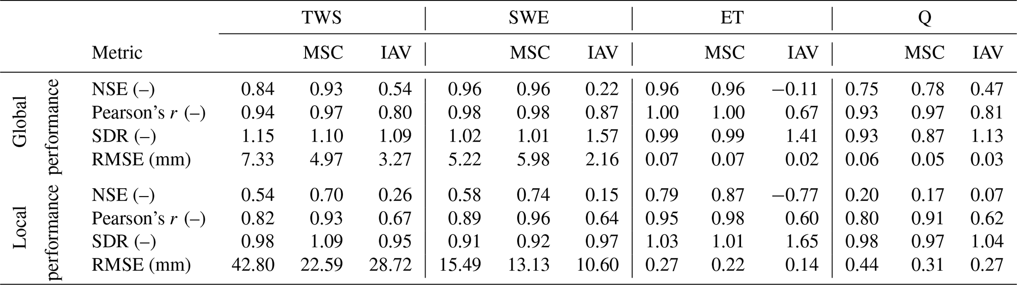
The model reproduced the patterns of the observed variables well (Table 3). In general, the global signal (global performance; see Eq. 26) was reproduced better than the local cell-level signal (local performance; see Eq. 27). For both observational constraint variables TWS and SWE, a NSE eNSE>0.8 and Pearson's correlation r>0.9 on the global level and eNSE>0.5 and r>0.8 for the local level was achieved. The seasonal signals of TWSMSC and SWEMSC were modeled with high accuracy (eNSE>0.9 on the global level; eNSE=0.7 on the local level) while the interannual variability performance varied. The TWSIAV was reproduced well with eNSE=0.54 (r=0.8) on the global level and with eNSE=0.26 (r=0.67) on the local level. The SWEIAV performance was decent for the global signal (eNSE=0.22; r=0.87) but lower (eNSE=0.15; r=0.64) on the local level.
Both ET and Q are machine learning model based and not directly observed at global scale. The patterns were reproduced well in terms of the seasonality on the global level, while the local performance was lower. For the ETIAV, a low NSE is achieved on the global level () and on the cell level (), while the correlation is still relatively good, with r=0.67 on the global level and r=0.6 on the local level. The SDR, the ratio of modeled and observed standard deviation, indicates that, on both the global and local levels the variability in the simulated ETIAV signal is substantially larger than the reference data with SDR of 1.41 on the global level and SDR of 1.65 on the cell level (see Fig. A2 in the Appendix for spatial patterns). For Q, the performance is decent on the global level and lower on the local cell level. Also here, low values in terms of NSE are accompanied by relatively good correlation. Because the independent data for ET and Q are not direct observations, we focus on TWS and SWE in the following. Maps of mean simulated versus observed fluxes and the spatial patterns of the model performance are provided in Appendix A.
Table 3The global (spatially averaged) and local (median cell level) model performance for the observational constraint variables terrestrial water storage (TWS), snow water equivalent (SWE), evapotranspiration (ET), and runoff (Q) and their decomposition into the mean seasonal cycle (MSC) and interannual variability (IAV). The Nash–Sutcliffe model efficiency (NSE), Pearson correlation (r), root mean square error (RMSE), and the ratio of modeled and observed standard deviation (SDR) are calculated for the test set, where values represent the mean across the 15 cross-validation runs. Positive values of SDR indicate that the modeled variance is larger than the observed. Note that, for the SWE, cells with constant 0 were dropped. The values were calculated for the test set in the range 2009 to 2014 on monthly timescale.
3.2 Benchmarking H2M against GHMs
For the quantitative benchmarking of H2M performance with the state-of-the-art GHMs from eartH2Observe (see Sect. 2.1.4), we use the common time period of 2009 to 2012 (not 2009–2014, as in the previous section) but all common grid cells between the GHMs and H2M. This is justified, as H2M has a negligible generalization error in space, i.e., the H2M performance is not systematically better in training grid cells. Similarly, we use the entire common time period (including the training data) for the qualitative assessment of the water cycle dynamics, as also in time, the generalization error was small. We note here that H2M was optimized with the datasets used for evaluation, while the GHMs have either been calibrated using catchment-level observational runoff data (LISFLOOD) or rely on prior parameter estimation (W3RA, SURFEX-TRIP, and PCR-GLOBWB) alone (Schellekens et al., 2017). The comparison presented here serves the purpose of performance benchmarking of the hybrid modeling approach rather than finding the best model.
The H2M modeling efficiency (i.e., the NSE) falls within the range of the GHMs in terms of the global performance (⋄ in Fig. 3), although the performance varies less across the variables and temporal scales. However, H2M achieves a consistently higher local performance (boxes in Fig. 3). The TWS is reproduced slightly better by the PCR-GLOBWB, which, however, has a relatively low performance on the local scale. All models struggle to reproduce the SWEIAV signal. The median NSE of H2M is on par with W3RA and SURFEX-TRIP, while the performance on spatially aggregated level is lower. A comparison of the model performance using the same forcings as in the eartH2Observe ensemble is provided in Appendix D.
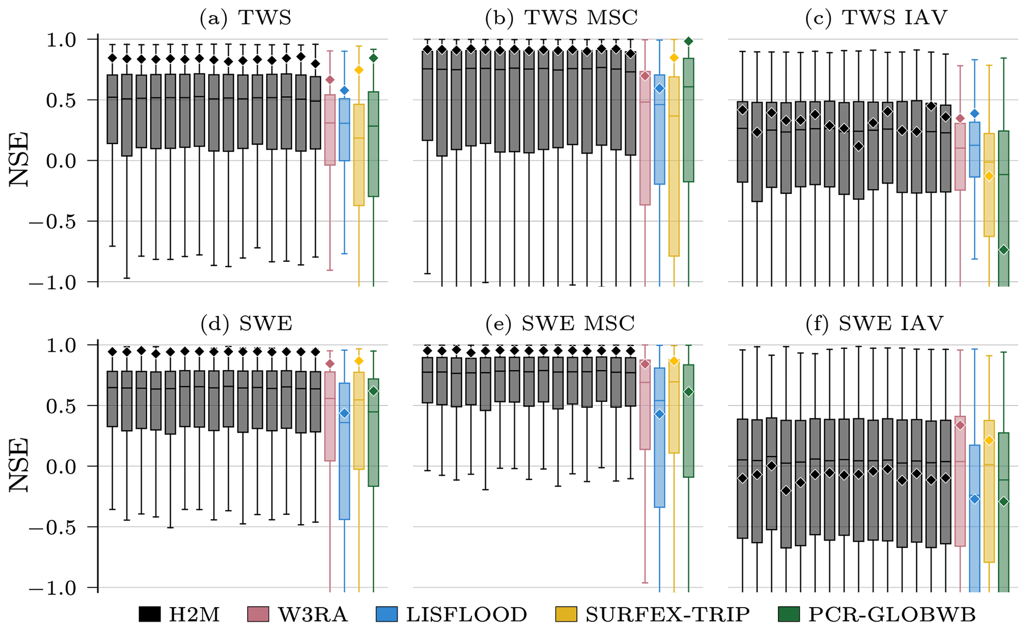
Figure 3Global and local grid cell level Nash–Sutcliffe model efficiency coefficient (NSE) of the hybrid hydrological model (H2M) and the process-based global hydrological models (GHMs) for the terrestrial water storage (TWS) on top and the snow water equivalent (SWE) at the bottom. The gray bars represent individual cross-validation runs. The ⋄ markers show the global (spatially averaged signal) model performance, and the boxes represent the spatial variability of the local cell level performance. The y axis was cut at −1 due to some large negative NSE values. The panels show the model performance with respect to the full time series, the mean seasonal cycle (MSC), and the interannual variability (IAV). Note that, for SWE, only grid cells with at least 1 d of snow are shown, as the NSE is not defined if the observations are constant zero, which would lead to a comparison of different grid cells. The metrics are calculated from the complete common time range from 2009 to 2012 on a monthly timescale. Note that deviations from the numbers reported in Table 3 are due to different time ranges.
While all models reproduce the global monthly and seasonal TWS (Fig. 4) relatively well, the results vary more substantially for the TWSIAV. Here, the H2M, WR3A, and LISFLOOD models show the best agreement with the TWS observations (also see Fig. 3 of the model performance). The lower agreement of SURFEX-TRIP and PCR-GLOBWB on the global interannual scale can be attributed to the time periods 2005–2006 and 2008–2010, respectively. From Fig. B1 of the regional averages (Appendix B), it becomes evident that this low agreement on global level is mainly due to a low agreement in the tropical regions (T1 – S-AM tropical; T2 – AFR tropical).
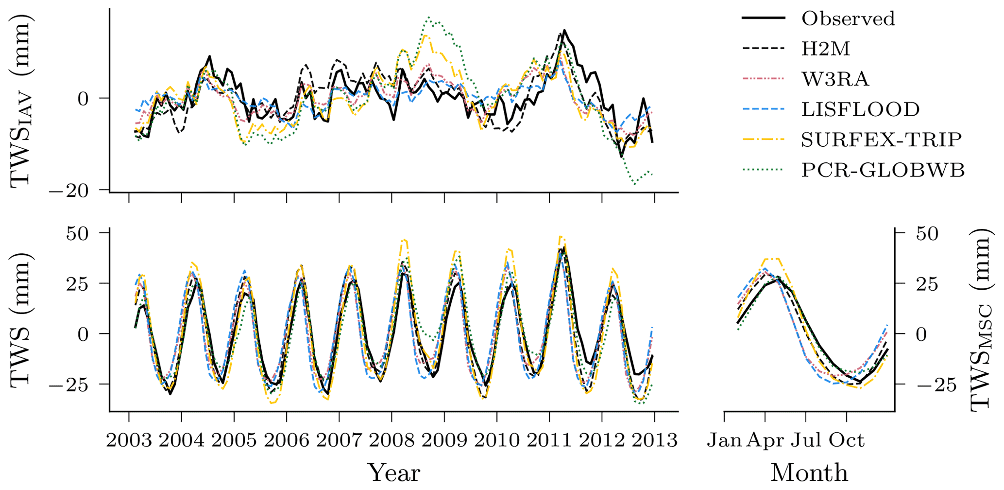
Figure 4Comparison of the hybrid hydrological model (H2M) and a set of process-based global hydrological models (GHMs) of the terrestrial water storage (TWS), its mean seasonal cycle (TWSMSC), and its interannual variability (TWSIAV) for the global signal. The time series were aggregated using the cell-size-weighted mean across all grid cells. The regional time series are show in Appendix B, Fig. B1.
The global SWE was well reproduced by H2M; in particular, the seasonal cycle showed better agreement than the GHMs, where the latter agreed well with the timing but not the magnitude (Fig. 5). The global interannual variability was not reproduced well by H2M, LISFLOOD, and PCR-GLOBWB. Interestingly, H2M performed best when forced by the same WFDEI data as in the GHM simulations (Fig. D1 in Appendix D). A regional model comparison of the time series are provided in Appendix B.

Figure 5Comparison of the hybrid hydrological model (H2M) and a set of process-based global hydrological models (GHMs) of the snow water equivalent (SWE), its mean seasonal cycle (SWEMSC), and its interannual variability (SWEIAV) for the global signal. The time series were aggregated using the cell-size-weighted mean across all grid cells. The regional time series are show in Appendix B, Fig. B2.
3.3 Hydrological responses in H2M
For the qualitative assessment of the hydrological responses, we use all grid cells, like in the previous section, and show the time range from 2003 to 2014 in time series plots. This involves the training data, but the impact is minimal due to a negligible generalization error. The H2M yields a set of data-driven, spatiotemporally varying coefficients that define the hydrological responses and generation of key hydrological fluxes. In particular, we focus on the following four parameters: αsoil, the fraction of throughfall that percolates into the soil, αgw, the fraction that recharges the groundwater, αsurf, the fraction that runs off as surface runoff component, and αet, the evaporative fraction (ratio of evapotranspiration to net radiation). Here, we analyze the spatiotemporal variability in the parameters and how they are associated with soil moisture condition defined by soil water deficit. In essence, these are analogous to stage–discharge relationships (Kumar, 2011) that are commonly used to characterize hydrological responses of river discharge at the catchment scale.
The partitioning of the liquid water input winp (rainfall plus snowmelt) by the fractions for soil recharge (αsoil), groundwater recharge (αgw), and surface runoff (αsurf) was robust across cross-validation runs and showed a clear relationship to CWD (Fig. 6). With an increasing soil water deficit (larger CWD; drier soil), the soil recharge increases, while the groundwater recharge and surface runoff decrease. For a CWD below 200 mm, we observe a large spatiotemporal variation in the partitioning, evident through the relatively large difference between the 20th and 80th percentiles. The transition from larger soil recharge to larger groundwater recharge and surface runoff is exponentially decreasing, i.e., the change is faster with lower CWD (wetter soil). Above a CWD of 200 mm (dry soil), the partitioning is constant in space and time with αsoil converging to 1, while αgw and αsurf converge to 0. The relatively large variation under wet conditions (low CWD) in Fig. 6 can be attributed about equally to temporal and spatial variability. The groundwater recharge fraction αgw shows a slightly larger temporal variability than the other fractions, and the contribution of the temporal component was generally a bit lower in the transitional regions.
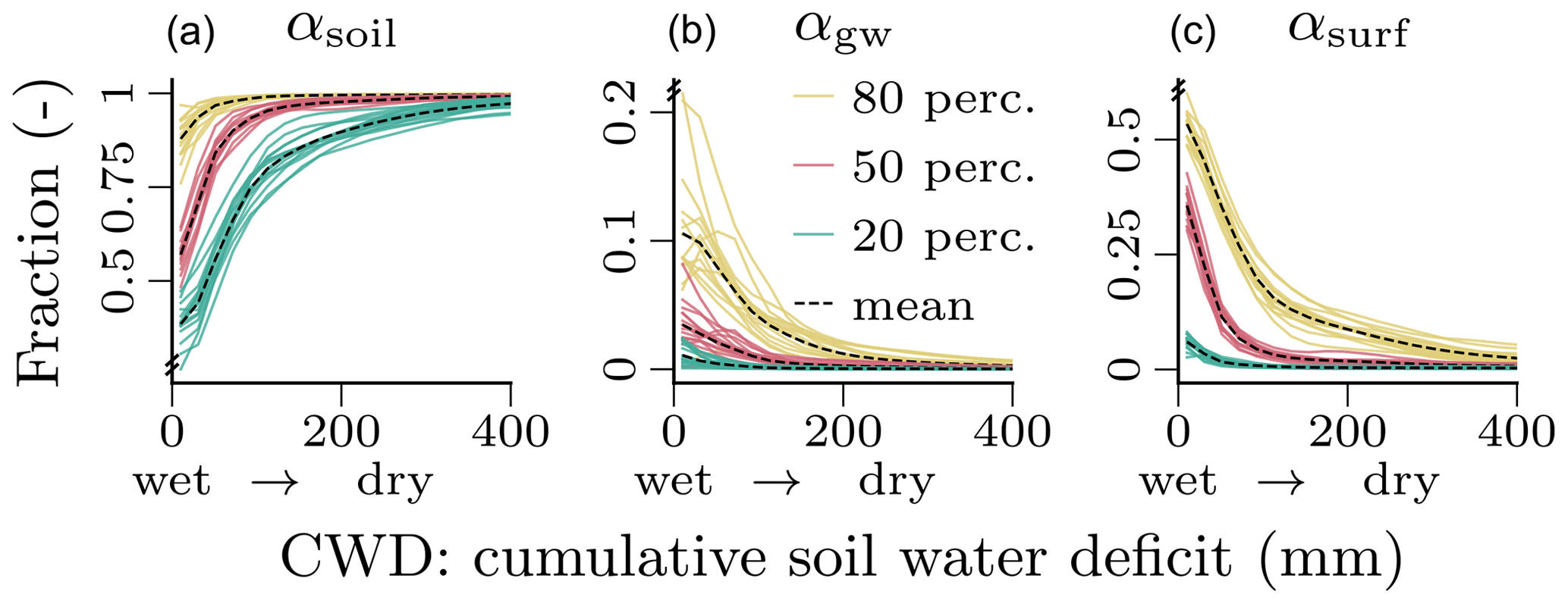
Figure 6Relationship between the water input partitioning fractions for soil (αsoil; a), groundwater (αgw; b) and surface runoff (αsurf; c), and the cumulative soil water deficit (CWD), as learned by the neural network. The figure shows the respective percentiles of the spatiotemporal conditional distribution , where C is the cumulative soil water deficit on the x axis discretized into N=10 bins . The colored lines show the percentiles per cross-validation run, and the black dashed lines show the mean across the colored lines. The CWD dynamics correspond to negative soil moisture, i.e., larger CWD for drier soils, and thus, a larger CWD corresponds to smaller soil moisture. The plots are based on global daily cell time steps from 2009 to 2014. Note the differences in the y scale.
In most hydroclimatic regions, αet showed a negative relationship to CWD under dry conditions (magenta lines in Fig. 7), and no relationship in presence of precipitation or snowmelt (green lines in Fig. 7). The high latitude and tropical regions showed a less clear relationship and less variation in CWD in general. In all regions, αet was close to 1 with large water input (win>5 mm). In arid (S1–2) and semiarid (N1–5) climates, αet exhibits a large range with steep gradients, given low water input (win=0 mm), decreasing with larger CWD (drier soil). The 10–90th percentile spread is large in most cases, which indicates that the relationship is modeled with a large spatiotemporal variability.
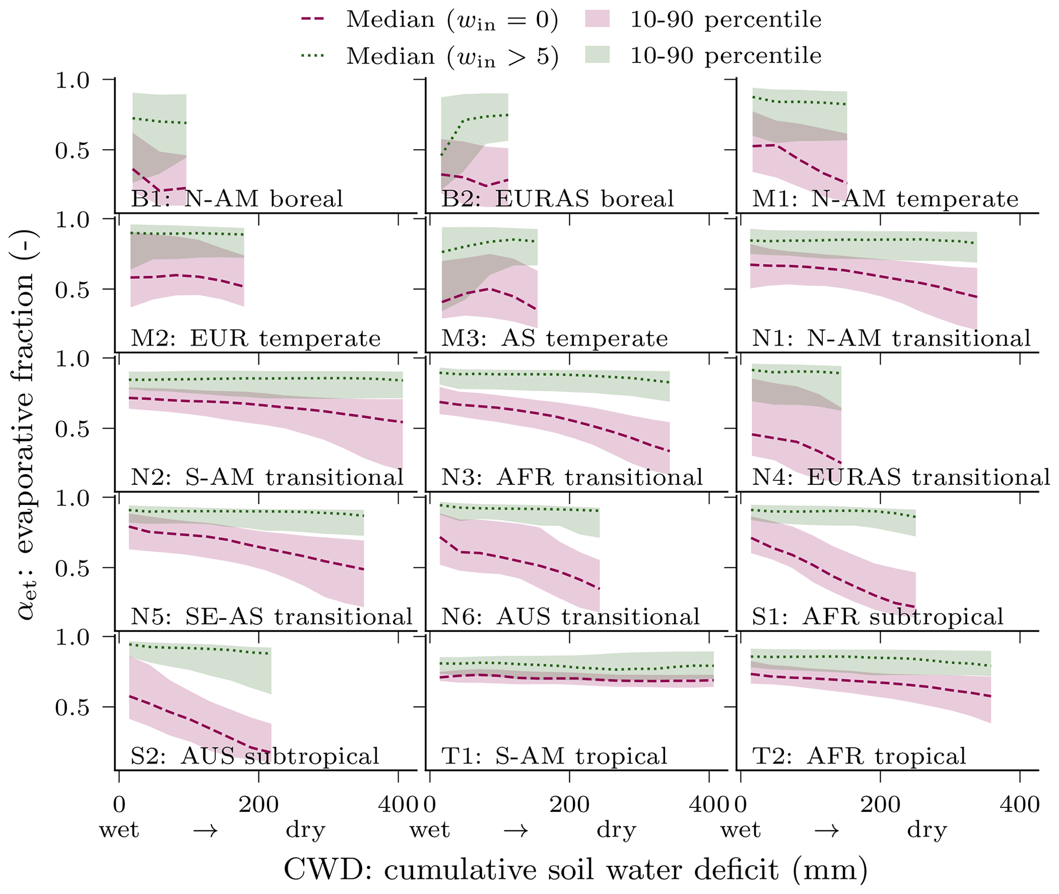
Figure 7Relationship between evaporative fraction (αet) and cumulative soil water deficit (CWD) for different hydroclimatic regions. The lines shows the respective percentiles of the spatiotemporal conditional distribution , where C is the cumulative soil water deficit on the x axis discretized into N=10 bins . The lines represent the median, and the 10 to 90th percentile is displayed as a shaded area. The red colors depict conditions without water input, , i.e., no precipitation or snowmelt, and green colors represent high water input larger than 5 mm, . Note that the CWD minimum was subtracted per grid cell. To exclude cells with a low CWD variability, only the cells in the top 60 % maximum CWD were used. The CWD dynamics correspond to negative soil moisture, i.e., a larger CWD implies drier soils. The plots are based on global daily cell time steps from 2009 to 2014.
The H2M shows a large water balance surplus of 12.9 and 21.4 mm yr−1, respectively, depending on the forcing dataset used (Table 4). The values are robust across cross-validation runs. The largest surplus occurs with the GPCP precipitation product, which is 9 mm yr−1 larger than WFDEI. The GHMs all show a lower ET and a larger Q trend than H2M.
Table 4Global yearly evapotranspiration (ET), grid cell runoff (Q), precipitation (Precip.), and storage change (Δ storage) over the period from 2003 to 2012 for the hybrid hydrological model (H2M) and a set of physically based global hydrological models (GHMs). The H2M was forced with the GPCP precipitation product (H2M) and the WFDEI data (H2M (WFDEI)) independently. The latter dataset is also used by the GHMs. The values for H2M and H2M (WFDEI) represent the mean ± the standard deviation across all cross-validation runs. Values from the common land-mask of all models were considered.

* GPCP for H2M or, otherwise, WFDEI.
The global parameters (β) were both estimated robustly, with a mean baseflow constant βgw=0.008 and a mean snow undercatch correction constant βsnow=0.77 and a relative standard deviation of 6 % and 2 % across the 15 cross-validation runs, respectively.
3.4 Terrestrial water storage composition
In this section, we show the TWS partitioning into snow, soil moisture, and groundwater variations as simulated by H2M and compare it with the corresponding partitioning from the GHMs.
The spatial patterns of the TWS partitioning vary strongly among the models (Fig. 8). Some patterns are consistent, though. The TWS seasonality (Fig. 8, top) is dominated by SWE in the high latitudes in all model simulations. Furthermore, all models tend to attribute the TWS variability to soil moisture in hot arid and semiarid climates. In other regions, the models diverge substantially. Both W3RA and PCR-GLOBWB attribute stronger groundwater contributions in most tropical and mild climates, while LISFLOOD and SURFEX-TRIP do not show much variation outside cold, semiarid, and arid regions. In H2M, only the humid Amazon region and Southeast Asia show a distinct contribution from groundwater. For the TWSIAV decomposition (Fig. 8; bottom), we see a rough agreement between the H2M, LISFLOOD, W3RA, and PCR-GLOBWB model in North America, Europe, and northern and central Asia. The latter two, again, show a stronger groundwater contribution, which extends to southern tropical and mild climates. The largest difference between H2M and the GHMs is the low H2M contribution of groundwater to TWSIAV in Africa, which could also be seen in the TWSMSC decomposition (Fig. 8; top).
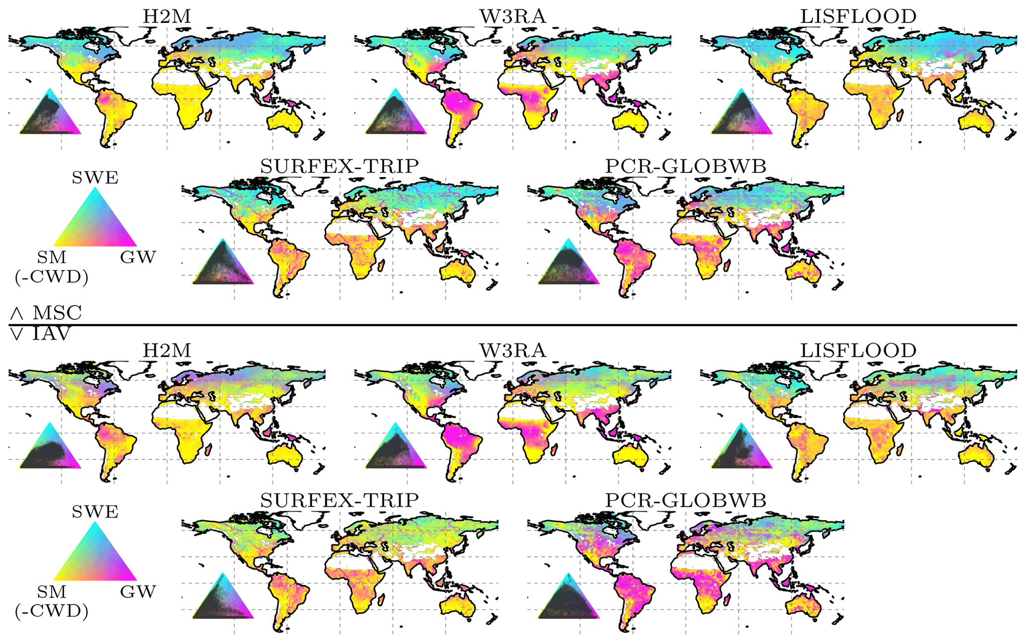
Figure 8Terrestrial water storage (TWS) variation partitioning into soil moisture (SM, corresponding to negative modeled cumulative water deficit, CWD), groundwater (GW), and snow water equivalent (SWE) by the hybrid hydrological model (H2M) and a set of process-based global hydrological models (GHMs). The top panel shows the partitioning of the mean seasonal cycle (MSC), and the bottom panel shows the interannual variability (IAV). The map colors correspond to the mixture of the contributions of the three variables, and the inset ternary plots reflect the density of the map points projected onto the components. The contribution is calculated as the sum of the bias-removed absolute deviance of a component from the mean, divided by the contribution of all components. Note that surface storage is included in the groundwater component for the models SURFEX-TRIP and PCR-GLOBWB. The decomposition is done based on the years 2003 to 2012.
Not only the spatial patterns of the TWS partitioning show large variations. Figure 9 illustrates the differences in amplitude and timing for the global time series and their decomposition into MSC and IAV. For the seasonal TWS signal, the amplitudes are qualitatively similar, and the main contribution comes from the snow. H2M, SURFEX-TRIP, and PCR-GLOBWB show a soil moisture slightly delayed to the snow seasonality and the groundwater peak setting in the late northern spring. W3RA shows very similar soil moisture and groundwater curves, which are slightly delayed to the snow seasonality, and LISFLOOD simulates groundwater and soil moisture in alternating cycles with only little variability. The IAV timings of the components are more consistent, but the amplitudes differ significantly across the models. The H2M attributes most TWSIAV to variations in soil moisture, while groundwater dominates the signal for PCR-GLOBWB. Note that the groundwater component also includes the surface water storage for the latter. Also, SURFEX-TRIP and PCR-GLOBWB both show a large global negative IAV anomaly from 2005 to 2006 and a positive one from 2008 to 2010, which are not observed by GRACE.
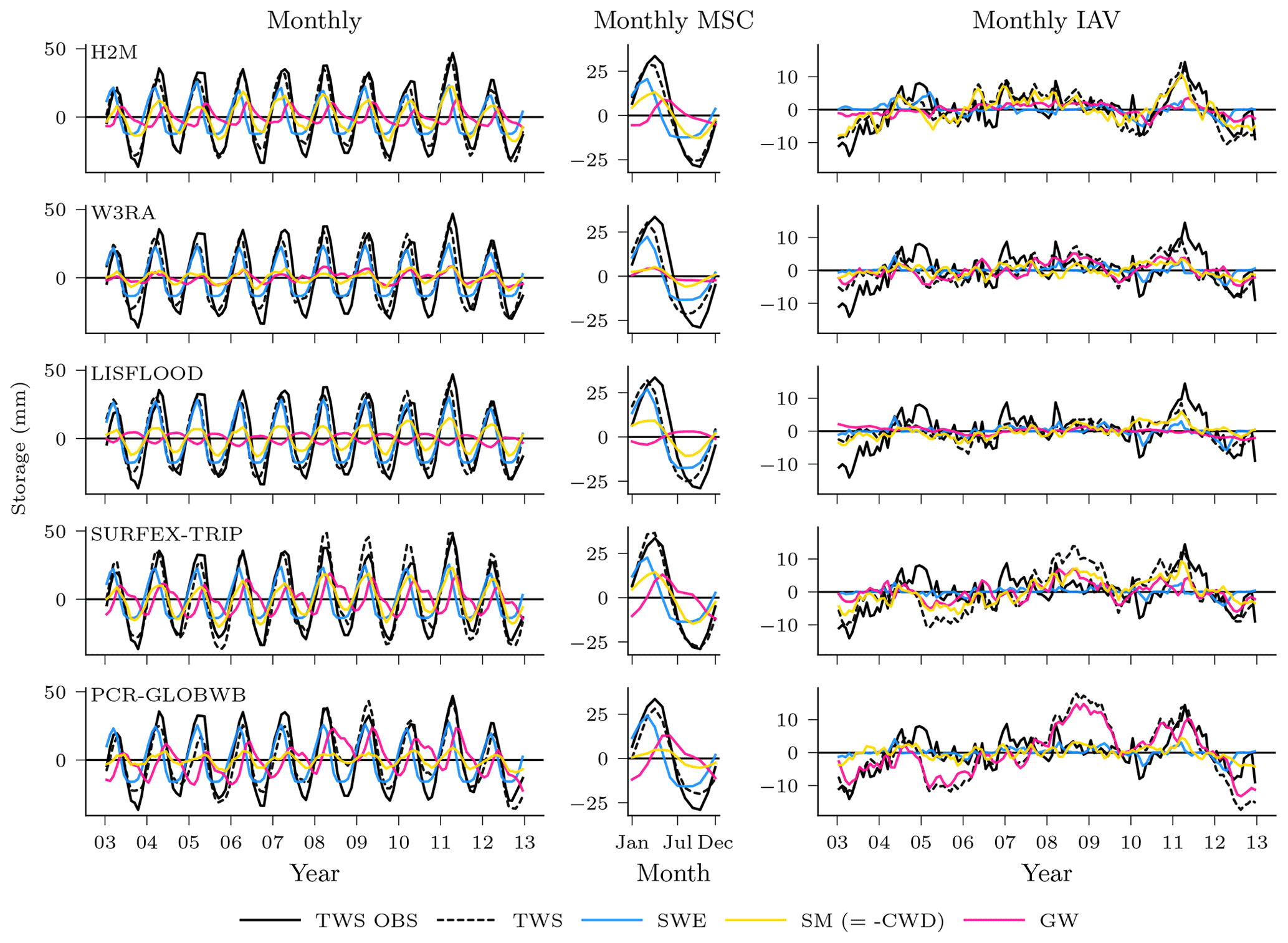
Figure 9Global variability in the terrestrial water storage (TWS) and the components snow water equivalent (SWE), soil moisture (SM), and groundwater (GW) for the hybrid hydrological model (H2M) and the process-based global hydrological models (rows). Note that SM corresponds to negative modeled cumulative water deficit (CWD) in H2M. For reference, the TWS observations are shown (TWS OBS). The monthly signal (left) and its decomposition into the mean seasonal cycle (MSC; center) and the interannual variability (IAV; right) are arranged in columns. The time series represent the global signal, i.e., the data were aggregated using the cell-size-weighted average per time step, and only cell time steps present in all model simulations were used. The y scale is consistent in columns but varies across the signal components. The training and test period is shown for the complete years 2003 to 2012. Note that surface storage is included in the groundwater component for the models SURFEX-TRIP and PCR-GLOBWB.
In this section, we briefly discuss the model performance and then assess the plausibility of a set of hydrological responses in H2M. We discuss the machine-learned relationship between CWD and runoff-generating processes, followed by an analysis of the CWD–αet (evaporative fraction) relationship. Then, we shed some light on the contrast of TWS composition between H2M and GHM simulations. Finally, we discuss general challenges and opportunities of the hybrid approach.
4.1 Model performance
The H2M simulations have a good agreement with the TWS and SWE observations despite the data biases. While some GHMs performed well at the global scale, H2M shows evidences of data adaptability at the local scale. This can be attributed to the data-driven patterns injected through the neural networks.
The TWS seasonality was reproduced well by H2M, except for extremely arid climates, with a low signal-to-noise ratio in observation, resulting in poor NSE values but also small RMSE and decent Pearson's correlation. The largest errors occur in humid regions with a stark TWS seasonality and large runoff rates, e.g., the Amazon basin, central Africa, and Southeast Asia (Fig. A1). This may be related to the missing representations of lateral flow or surface water storage variations in general, which can be important TWS contributions in humid environments (Kim et al., 2009; Scanlon et al., 2019) but also to data biases. A near-perfect fit was achieved for the globally averaged SWE seasonality (Fig. 5), while the local performance varied strongly across regions with the poorest performance in extremely cold tundra (Fig. B2). The SWEIAV is highly sensitive to the precipitation forcing data, which is highlighted by substantially better agreement with GlobSnow when H2M was forced with the WFDEI dataset (Fig. D1 in Appendix D).
In the hybrid modeling framework, the quality of the observational constraints is a major source of uncertainty. The data used in this study have well-documented deficiencies. The precipitation product, for example, shows large uncertainties in Africa due to limitations in density and quality of measurement sites (Sylla et al., 2013) and exhibits biases in snowfall estimates in the Northern Hemisphere due to over-correction of snowfall under catch (Behrangi et al., 2016; Panahi and Behrangi, 2019). The GlobSnow SWE saturates above 120 mm and underestimates the interannual variability (Luojus et al., 2010). TWS quality is generally difficult to quantify, as an equivalent ground-based measurement does not exist, and its complex preprocessing has known impacts on the data quality (Scanlon et al., 2016). The machine-learning-based constraints of Q and ET are not directly observed, and thus, they are expected to have considerable global and regional uncertainties and biases (Ghiggi et al., 2019; Jung et al., 2020). This could lead to inconsistencies in the water balance (Trautmann et al., 2022). However, the multi-objective optimization may dampen the negative effects of biases, as the model can trade off the different constraints.
4.2 Model interpretability
In this section, we assess the model interpretability, i.e., the plausibility of the hydrological responses that emerge from the machine-learned coefficients which have not been prescribed a priori. We discuss the partitioning of water fluxes and their dependence on antecedent soil moisture condition and then evaluate the partitioning of water storage contributing to TWS dynamics.
4.2.1 Hydrological responses
The H2M-learned hydrological responses to soil moisture states that are consistent with the hydrological understanding, and the learned coefficients are estimated robustly across cross-validation runs. The fact that these patterns are an emerging behavior constrained by a basic physical constraint of mass balance, i.e., the relationships were not explicitly predefined, is an encouraging finding that justifies the usage and further investigation of the hybrid approach in general.
The partitioning of incoming water into surface runoff and recharge of the soil and groundwater shows a clear nonlinear response to soil dryness (Fig. 6). The fraction of surface runoff (αsurf) decreases rapidly with increasing dryness while soil recharge (αsoil) increases correspondingly. Groundwater recharge occurs under wet conditions and approaches zero with increasing soil dryness. This runoff-generating process response to soil moisture qualitatively matches the expected behavior implemented in GHMs (Bergström, 1995).
The H2M predicts a large spatiotemporal variability in the soil-moisture-dependent runoff–recharge partitioning, as indicated by different percentiles in Fig. 6. For example, under moist conditions, more than 50 % of water input (blue lines in Fig. 6) or hardly anything (yellow lines) can be directed to surface runoff. Such large variability in the response can be expected due to large variations of topography, soil, and vegetation properties that control the infiltration–runoff response. The H2M approach, therefore, appears to offer perspectives in capturing the large natural variability in the effective runoff-generating process response. Note that these processes have been challenging to parameterize in traditional GHMs (Döll and Flörke, 2005; Beck et al., 2016, 2017; Koirala et al., 2017), and thus, the hybrid approach can fill in critical process gaps and long-standing physical modeling challenges.
The learned relationship between evaporative fraction (αet) and soil dryness (Fig. 7) is generally consistent with the demand–supply framework for evapotranspiration (Budyko, 1974). Under wet conditions, ET scales with atmospheric demand represented by net radiation, while evaporative fraction declines with increasing dryness, which is most clearly seen in the semi-arid regions of Australia and Africa. The learned relationship between αet and soil moisture response functions appears to be rather gradual as opposed to an idealized piecewise function with a clear soil moisture threshold that is still frequently employed in process models (Seneviratne et al., 2010; Schwingshackl et al., 2017). However, an about-constant potential evaporative fraction was predicted when there was substantial rain (or snowmelt), independent of the soil moisture state (green lines in Fig. 7). This shows that the model implicitly accounts for wetting of the top soil layers, which alleviates water stress even though it represents soil moisture (expressed as negative CWD) as a single bucket. The specific response of evaporative fraction predicted by H2M varies substantially between regions and within regions indicated by the shading in Fig. 7. Vegetation storage capacity has long been identified as a key uncertainty in the process models in controlling soil moisture stress responses (Ichii et al., 2009). Our approach in H2M avoids such explicit parameterizations of relatively less understood physical processes, and its effectiveness is supported by better performance of H2M in simulating TWS variations in tropical and subtropical regions compared to GHMs (Sect. 3.2), despite its simple overall structure.
4.2.2 Terrestrial water storage composition
As reported previously (Andrew et al., 2017) and as presented here, the attribution of TWS variations is a challenge that is yet to be met in global hydrology. The fact that all models disagree largely with respect to the decomposition was the main motivation to use an alternative, data-driven hybrid approach. The decomposition patterns simulated by H2M are reasonable, although the ground truth for a quantitative assertion is missing. The H2M simulations agree with the GHM, especially in regions where the decomposition is well constrained, which is an encouraging finding. In the tropical and semi-arid to arid regions, the decomposition is less clear. Here, all models disagree, although the larger soil moisture variations versus smaller groundwater variation is a unique feature of the H2M simulations. This may indicate that H2M is under-constrained in these regions. Or, the differences could result from a more accurate representation of the involved processes due to the local adaptivity of H2M. Most likely, it is a combination of both.
The dominant contribution of the SWE to seasonal cycle of TWS in the high latitudes (Figs. 8 and 9), but a lower contribution to the interannual variability is consistent across models and has also been previously reported (e.g., Rangelova et al., 2007; Trautmann et al., 2018). It should be noted that the SWEIAV was reproduced poorly by all models, reflecting large uncertainties in the input precipitation and SWE observations. Despite regional differences, the models also consistently attribute most of the TWS seasonal and interannual variability to soil moisture in arid and semi-arid regions (Fig. 8). The dominance of soil moisture is plausible in these regions, as the potential evapotranspiration is high, and precipitation is low and infrequent or strongly seasonal (Nicholson, 2011). Given the absence of secondary moisture sources, such as lateral flow and a lack of deep-rooted plants, most of the storage variations occur within a shallow soil depth (Grayson et al., 2006).
In other regions, the partitioning between groundwater and soil moisture variability is less clear. On both the seasonal and interannual scales, groundwater contributions to TWS correlate with humidity at the global scale (Feddema, 2005). In the boreal humid regions of northwestern North America, Scandinavia, and northwestern Russia, as well as the northeastern Asian coast, the groundwater contribution to TWS is larger than that of soil moisture. Here, groundwater recharge is concentrated in spring, with large snowmelt (Fig. 9) co-occurring with low evaporative demand due to low temperatures, irradiation, and vegetation productivity, which results in a large water surplus (Jasechko et al., 2014). The boreal regions with stronger soil moisture contribution are the ones affected by permafrost, where most of the vertical movement is limited to the thawed topsoil, and horizontal baseflow is usually lower than in non-permafrost soils (Bui et al., 2020). Thus, the patterns diagnosed by H2M are plausible. It must be noted, however, that significant drainage of the surplus water happens via river flows and lateral transport, which are not represented in H2M.
The large groundwater contribution on both seasonal and interannual scales in humid regions has been diagnosed by all models. In the tropics, the largest difference between H2M and the GHMs is the larger soil moisture contribution in the African rainforest simulated by H2M. The lower groundwater variability is – to a certain extent – reasonable, as the central Amazon and Southeast Asian rainforests are the most humid regions globally, with the largest annual precipitation (Zelazowski et al., 2011) and a shallow plant rooting depth, while the African rainforest is relatively drier and has deeper plant roots (Yang et al., 2016; Fan et al., 2017). However, the soil moisture variability is only marginally larger in H2M, while it is mainly the low groundwater amplitude that makes the difference (Fig. B3 in Appendix B).
In the arid-to-wet transition regions of Africa, H2M diagnoses only marginal groundwater variability compared to larger amplitudes in the GHMs. The H2M resolves the water balance mainly using soil moisture variations, i.e., through soil recharge and evapotranspiration, while the soil overflow was negligible. While the patterns found by H2M are within those of GHMs in most regions, the notable strong soil moisture contribution in tropical savanna and humid subtropical climates is unique in H2M.
GHMs require a large number of parameters that are either empirically derived or based on remote sensing or statistical datasets, e.g., plant functional types, root zone depth, soil texture maps, or soil thermal and hydraulic properties. Often, the said parameters are uncertain and may not necessarily represent a process at spatial scale of GHMs (scale mismatch) or within grid or catchment variabilities (sub-grid to local heterogeneity). Thus, simple heuristics have been used to parameterize hydrological processes, which can, in reality, be of high complexity (Beck et al., 2016). It has been suggested that GHMs underestimate the land water storage capacity in general and that especially the variability in deeper soil is too low (Zeng et al., 2008). In addition, the link between deeper soil layers and plant transpiration through root water uptake is often not represented adequately in GHMs (Jackson et al., 2000), although such effects have been found to play an important role in below-surface water variability (e.g., Kleidon and Heimann, 2000; Koirala et al., 2017). Compared to the GHMs, H2M provides a novel avenue on which storage variations are less bound by, presumably, ad hoc prescriptions of the size of soil and other storages. The diagnosed patterns of soil and groundwater variations, therefore, emerge from observation-based variations in water storage and fluxes. The H2M approach that also implicitly learns the layering of the soil, thus, can be used to address uncertainties in the moisture storage capacities (Zeng et al., 2008; Scanlon et al., 2019) and plant rooting depth (Yang et al., 2016) used in GHMs, which are likely to have a strong influence on the TWS partitioning.
The smaller groundwater contribution in H2M is also potentially related to the missing mechanisms of capillary rise and root water uptake from the groundwater. Thus, the cumulative water deficit dynamics implicitly represent all the below-ground water that will be returned to the atmosphere by root water uptake and transpiration at some point. As a possible consequence, H2M diagnoses larger soil moisture in transitional and especially in the subtropical regions but, more evidently, smaller groundwater variability.
Finally, the missing (explicit) representation of surface water and river storage may cause biases in H2M simulations. Surface storage has been found to contribute significantly to the TWS variations (Güntner et al., 2007; Scanlon et al., 2019), and a proper representation thereof is desirable. Furthermore, lateral water influx across a cell via rivers is not represented and may have a significant impact on the TWS composition (Kim et al., 2009).
4.3 Challenges and opportunities
The data-driven character of the H2M offers a set of opportunities but is accompanied by challenges. The H2M makes use of observational data streams that are not typically used in GHMs. However, to retain the interpretability of the predicted coefficients, the model structure must be kept simple; the model flexibility needs to be compensated with a simple causal model structure. Still, the H2M offers a great opportunity to study the hydrological cycle from a different viewpoint that is strongly rooted in the observation-based datasets, which are growing in availability at an unprecedented rate in the era of Earth observation.
The hydrological pathways in H2M are rather simple compared to GHMs, but the model still expresses a high data adaptivity, as demonstrated. While GHMs usually represent a wide range of hydrological sub-processes (e.g., infiltration, preferential flow, and topographical runoff–run on), the hybrid model integrates them to a few response functions, and the model complexity and interactions within are, so to speak, outsourced to the neural network. Still, missing representations of storage components (e.g., surface storage) and hydrological pathways (e.g., streamflows) limit the model flexibility and can, to a certain extent, corrupt the other latent variables as the model tries to accommodate for missing processes. Thus, the estimated coefficients in the current H2M implementation should be treated with some skepticism. At the same time, the relaxation of assumptions can be seen as an opportunity, as the prior knowledge used in GHMs may be wrong or incomplete. The impact of trading prior knowledge and model complexity with more flexibility and a data-driven approach on model uncertainties is a key aspect that needs further investigation.
As the model behavior emerges largely from the observational data constraints, the hybrid approach constitutes a novel technique for studying TWS variations. While purely data-driven approaches (see Andrew et al., 2017, for an overview) are generally useful as they provide insights independent from GHMs, they are based on strong qualitative assumptions (e.g., the temporal characteristics of the components at different depths), and they do not allow the incorporation of physical knowledge, principles, and constraints. GHMs themselves largely rely on prior knowledge, which may be false or incomplete, and the model parameterization is usually not resolved regionally, resulting in model uncertainties (Beck et al., 2016) which are eventually expressed in the disagreement among model simulations. The hybrid model can be seen as a compromise between the purely data-driven and the physically based approaches, as physical principles (e.g., mass conservation) are respected, but qualitative assumptions on the processes are still used.
Global hydrological models are often used for different tasks, such as the assessment of the water cycle at past and present, predictions for the future for evaluating implications of, e.g., land use changes by scenarios, and to gain process understanding. In principle and technically, a global hybrid hydrological model can be applied for the same tasks, while related simulations need to be interpreted with care. The strongest use case of H2M is the assessment of recent variations in the water cycle, since it can act as a physically consistent, yet data-adaptive, bridge between heterogeneous global data streams, and it complements traditional data assimilation approaches. Interpreting predictions too far into the past or future can be risky when factors that are not represented physically play a role that had little impact during the training period (e.g., permafrost melting and CO2 fertilization of water use efficiency). Likewise, it could make sense to conduct scenarios of, for example, different land use if the conditions represented by the scenarios have been represented during the machine learning in some way, while there always remains the danger that learned relationships by the neural network are just statistical associations rather than causal relationships (shortcut learning; Geirhos et al., 2020). As we could show, gaining process understanding from the hybrid model can be feasible as the spatially and temporally varying coefficients learned by the neural network are plausible and partly very interesting. However, such uncovered patterns may rather represent hypotheses that should be tested with complementary approaches like physical process modeling, direct observations, or experiments.
Improving the model through a better representation of the process complexity is an obvious next step. Several processes were not explicitly represented, such as overland flow, soil moisture recharge from the groundwater through capillary rise, or snow sublimation. The under-complex representation of certain processes leads to biases and uncertainties. For example, estimating the baseflow parameterization on cell level could improve the representative power of the model, as has been shown by Beck et al. (2013). This is, however, challenging as an increasingly complex model needs to be complemented by additional data constraints or better physical processes in order to avoid parameter equifinality issues that lead to the same or similar model responses across a large range of parameter values. It is also possible that the decomposition into CWD and GW is not properly constrained under some circumstances, e.g., in ecosystems that are not water limited. Here, either the groundwater or the soil moisture may be restored as needed (due to frequent precipitation) to match the observation of terrestrial water storage. More research is needed to address these problems, particularly a complementary development of application-based models, as presented in this study, and smaller-scale, better constrained exercises to advance hybrid modeling can be a viable alternative.
Closely related to equifinality is the quantification of model (epistemic) and data (aleatoric) uncertainties. A proper representation of model uncertainties would enable a direct identification of equifinality and allow a targeted model development for uncertain processes. The implementation of such a mechanism could be built into the neural network, e.g., by using Bayesian deep learning (Wang and Yeung, 2020) or deep generative models (Goodfellow et al., 2016). Explicit consideration of data uncertainty will also be beneficial, either to propagate forcing data uncertainties through the model or to model the uncertainties of the observational constraint variables, which is not always provided. Data assimilation is a framework that allows representing such uncertainties (Reichle, 2008) and can even be extended to incorporate model parameter estimation (Moradkhani et al., 2005), i.e., learning physical processes as in the hybrid approach presented here. In contrast to data assimilation that often targets improving prediction skills, the goal of hybrid modeling is to develop a generalizable model, which can be applied beyond the specific forecasting task in data assimilation. Nevertheless, non-parametric machine learning approaches can also be included into data assimilation as discussed in Geer (2021).
The rapid development of novel products opens interesting opportunities, like a daily TWS product (Kvas et al., 2019) can help to better constrain sub-monthly water processes. Furthermore, the upcoming Surface Water and Ocean Topography (SWOT) mission, which is targeted at observing surface water storage variations (Biancamaria et al., 2016), could be useful to solve current shortcomings of the H2M. In addition, parameters estimated by other approaches, such as the upscaled baseflow index (Beck et al., 2013), offer interesting independent constraints that allow the addition of further complexity to the model without increasing the uncertainty.
Finally, incorporating lateral interactions and flow between grid cells (e.g., large-scale groundwater flow and river routing) are outstanding but relevant challenges, as the paradigm of optimizing neural networks with randomized samples that are independent will likely not be sufficient in modeling connections and interactions between regions. Such endeavors would also allow for bringing in established global datasets of river discharge measurements such as provided by the Global Runoff Data Centre (GRDC; Fekete et al., 1999).
The present study demonstrates the strengths of combining machine learning and physical process understanding for global hydrological modeling. The main conclusions of this study are as follows:
-
The hybrid model is capable of obtaining similar performance to physically based models at global level but achieved better local adaptivity. This highlights the strengths of the hybrid approach, which can replace complex physical processes, integrate different datasets, and is highly data-adaptive due to the model parameterization by a neural network.
-
The model simulations were plausible and followed basic hydrological principles. This is partially due to the physical constraints, which force the model into physical consistency (e.g., conservation of mass), but is also emerging from the multiple data constraints.
-
The hybrid model partitioning of the terrestrial water storage into its components yielded plausible and interesting patterns. The agreement of the decomposition is generally high in regions where the physically based models are more consistent (e.g., temperate, semi-arid, and arid regions), but generally, the hybrid model shows a larger contribution by soil moisture.
-
Key opportunities and challenges in hybrid modeling to be addressed in the future are identification of equifinality, quantification of uncertainties, integration of multi-resolution datasets, and representation of cell neighborhood effects, such as lateral fluxes.
Hybrid modeling has the potential to advance the Earth sciences by providing an alternative perspective to knowledge-driven approaches. The data adaptivity can reveal the weaknesses and strengths of process-based models and provide important insights for water cycle attribution and diagnostics. The findings and methods of this study can be generalized to other spheres and scales across the Earth system, as long as sufficient data and process knowledge are available.
Overall, high NSE of TWSMSC is achieved in most regions (Fig. A1). Low TWSNSE hot spots are primarily found in some arid regions with little overall TWS variability, e.g., the Namib desert in southern Africa or the Gobi desert in eastern Asia. In terms of the RMSE, regions with larger variations in TWS dominate with the largest MSC error in the Amazon and less expressed in southeastern Asia. The correlation (r) was constantly well above 0.5 for TWSMSC, except for the Gobi Desert, where the TWS variations are minimal. The TWSIAV was also reproduced well in terms of r.
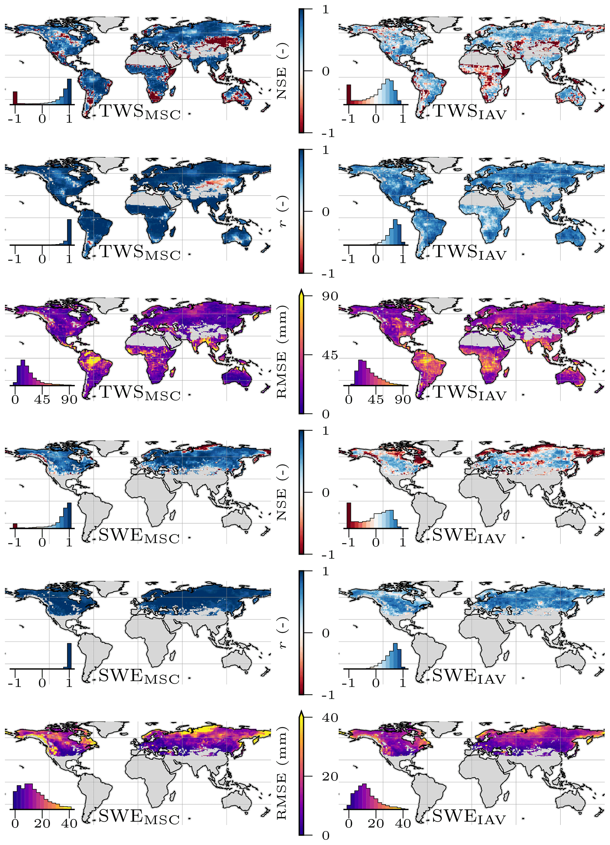
Figure A1Local model performance for terrestrial water storage (TWS) and snow water equivalent (SWE) on the mean seasonal cycle (MSC) and the interannual variability (IAV) within the test period (2009 to 2014). The Nash–Sutcliffe model efficiency (NSE), Pearson correlation (r), and root mean square error (RMSE) are shown. The inset plots show the cell-area-weighted histogram of the map values.
The SWEMSC is reproduced well in terms of NSE and r, while NSE for SWEIAV is low, especially in tundra regions (Fig. A1). The RMSE is also larger in high latitudes but more concentrated in regions with large seasonal amplitudes.
The average patterns of states (TWS and SWE) and fluxes (ET and Q) were reproduced well in general (Fig. A2). The model underestimates the variability in TWS in central Amazon, West Africa, and India. These patterns align well with the occurrence of large rivers (e.g., Amazon, Ganges, Mississippi, Niger, or Yenisei) and may be caused by missing representation of river routing. The SWE is overestimated in the extremely cold regions of North America and Northeast Asia and underestimated in tundra regions. Average Q is largely underestimated in Central Africa and slightly overestimated in northwestern Eurasia, central Amazon, and coastal regions of Australia and East Asia. ET, finally, is underestimated by the model, prominently in most of sub-Saharan Africa and East Brazil, while no major biases are present in other regions.
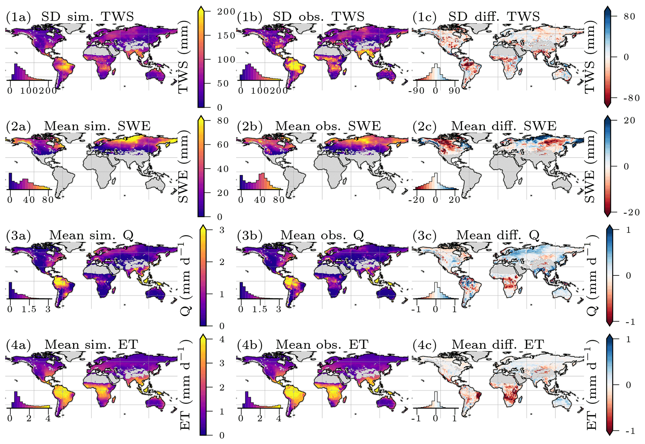
Figure A2Mean (a) simulated, (b) observed, and (c) the difference of simulated minus observed (positive means simulated is larger) terrestrial water storage (TWS; 1a–c), snow water equivalent (SWE; 2a–c), total runoff (Q; 3a–c), and evapotranspiration (ET; 4a–c). Note that, for the TWS, the standard deviation is shown as the values represent variations around the mean. The inset histograms represent the map value distributions, and the mean for the test period (2009 to 2014) is shown.
On a regional scale, most models reproduced the TWSMSC well (eNSE>0.5), while the TWSIAV performance varied (eNSE<0.5) (Fig. B1). The variation between models was larger in terms of IAV, especially in transitional and tropical zones. Especially the TWSIAV seems to be reproduced poorly in certain regions by all models, e.g., temperate Asia (M3), transitional Africa (N3), Eurasia (N4), and Southeast Asia (N5). In the high latitudes, we observe a phase difference of the simulated TWS compared to the observations for all models except the PCR-GLOBWB.
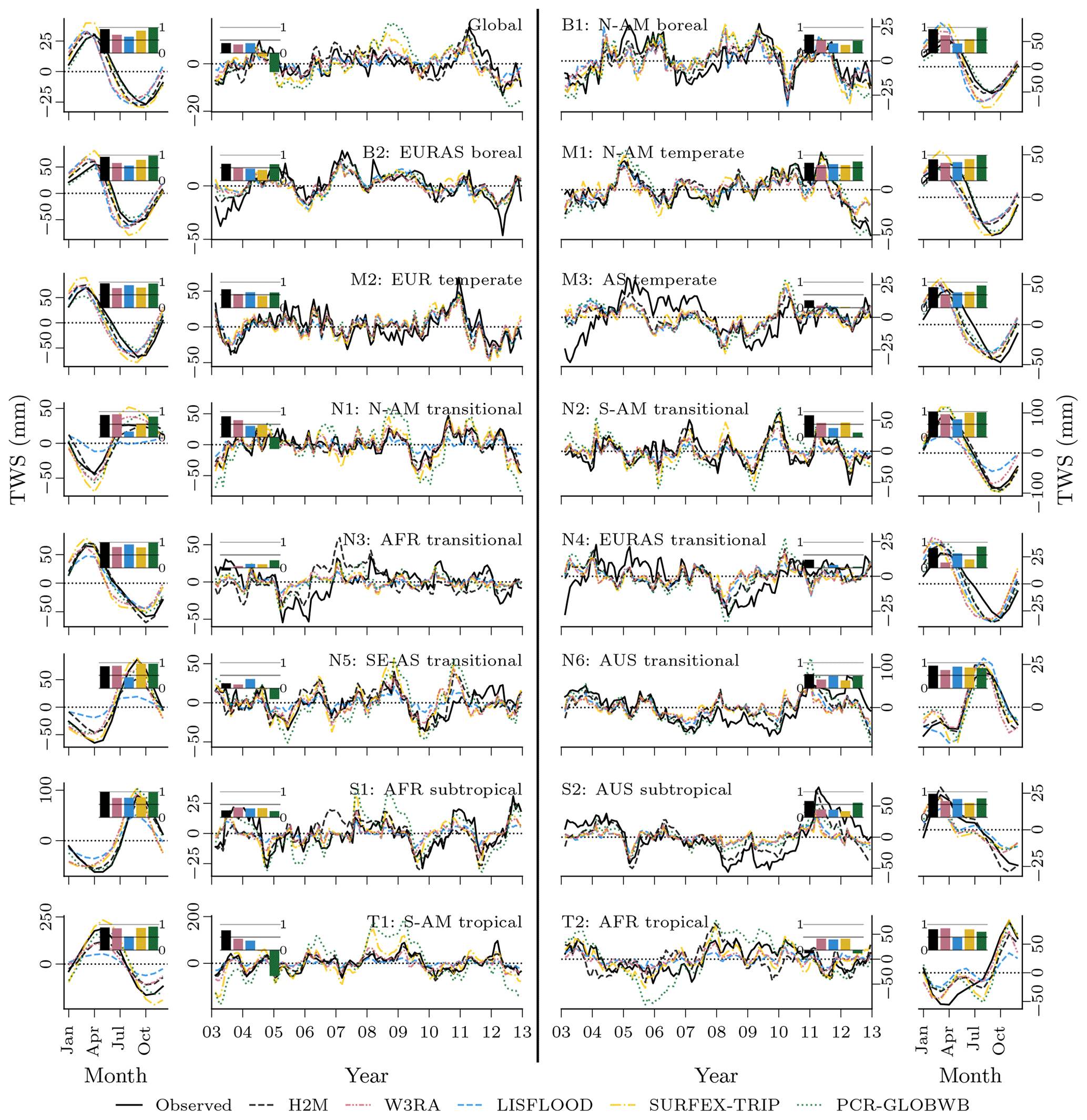
Figure B1Comparison of the hybrid hydrological model (H2M) and a set of process-based global hydrological models (GHMs) of the terrestrial water storage mean seasonal cycle (TWSMSC; outer columns) and interannual variability (TWSIAV; center columns) in millimeters for hydro-climatic regions (Fig. 2). The time series were aggregated using the cell-size-weighted mean across all grid cells in the respective region. The inset axes show the Nash–Sutcliffe model efficiency (NSE) of each model with the same color-coding as the time series. Note that the y scale differs between plots.
Most models manage to reproduce the SWEMSC well, with an eNSE>0.5, while the SWEIAV performance is more variant and lower in general (Fig. B2). We note a phase difference between the model simulations and observations that is most notable in the boreal regions, indicating that the models either accumulate too much snow during winter or do not manage to discharge it in spring or both. The phase difference is less expressed in H2M and lowest in PCR-GLOBWB. The SWEIAV varies strongly across different regions. The SWEIAV has strong seasonal variations, with opposite patterns in different regions that cancel each other out on a global level. This is evident on the regional anomalies and results in low variability at the global scale. In general, all models reproduce the sign of anomalies better than the amplitudes.
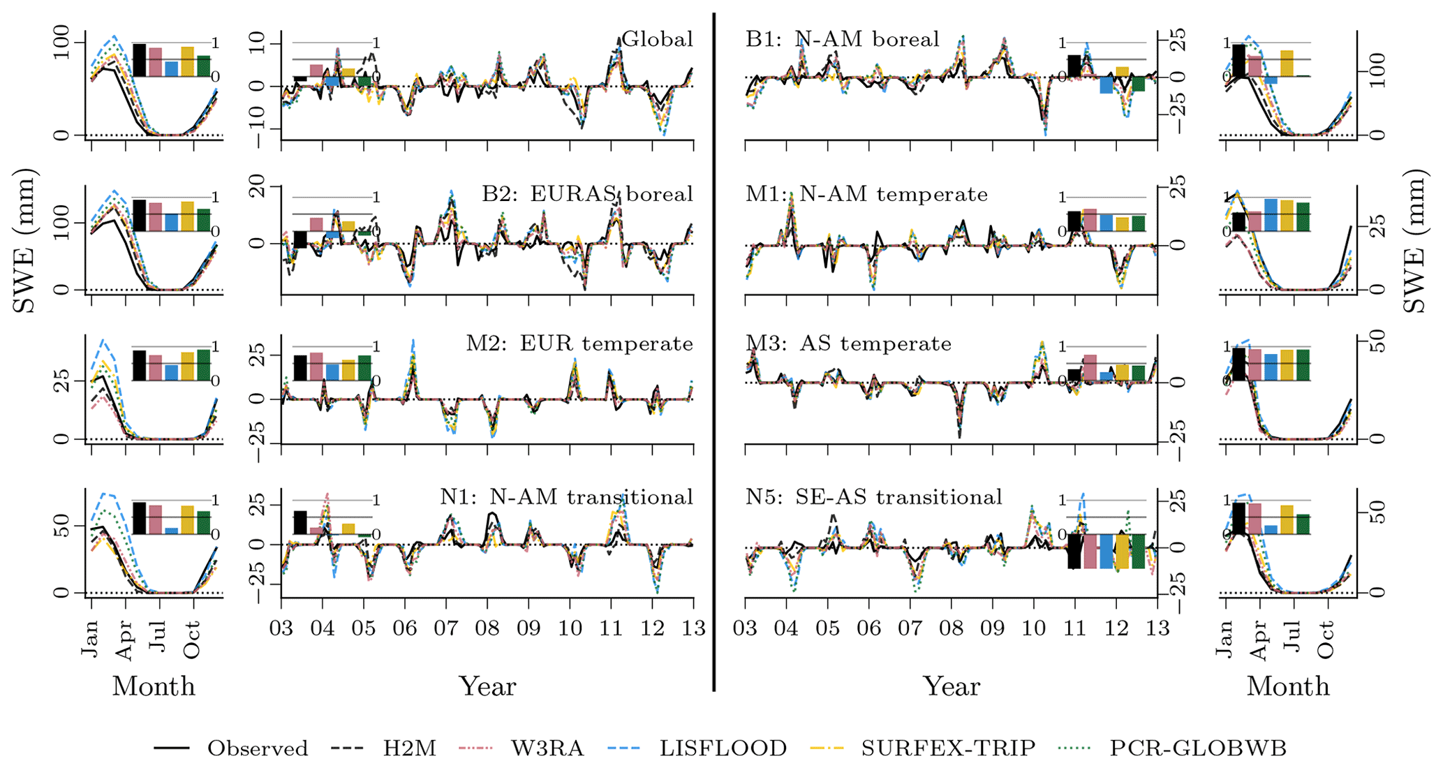
Figure B2Comparison of the hybrid hydrological model (H2M) and a set of process-based global hydrological models (GHMs) of the snow water equivalent mean seasonal cycle (SWEMSC; outer columns) and interannual variability (SWEIAV; center columns) in millimeters for hydro-climatic regions (Fig. 2). The time series were aggregated using the cell-size-weighted mean across all grid cells in the respective region. The inset axes show the Nash–Sutcliffe model efficiency (NSE) of each model with the same color-coding as the time series. Note that regions without snow dynamics are not included. The y scale differs between plots.
The regional-scale seasonal anomalies of simulated soil moisture (corresponding to negative CWD in H2M) and GW show a more detailed picture of the model variabilities (Fig. B3). The global-scale SM amplitude of H2M is larger than the one of the GHMs (although close to the SURFEX-TRIP model), while the GW variations are smaller in H2M. The largest discrepancies between H2M and the GHMs are in the northern (N1) and southern (N2) America transitional, the Australian subtropical (S2), and the African tropical (T2) regions. However, also the within GHM variation is large in most regions. The model simulations agree relatively well in the temperate regions (M1–3) and in the Africa (N3), Eurasia (N4), and Australia (N6) transitional zones.
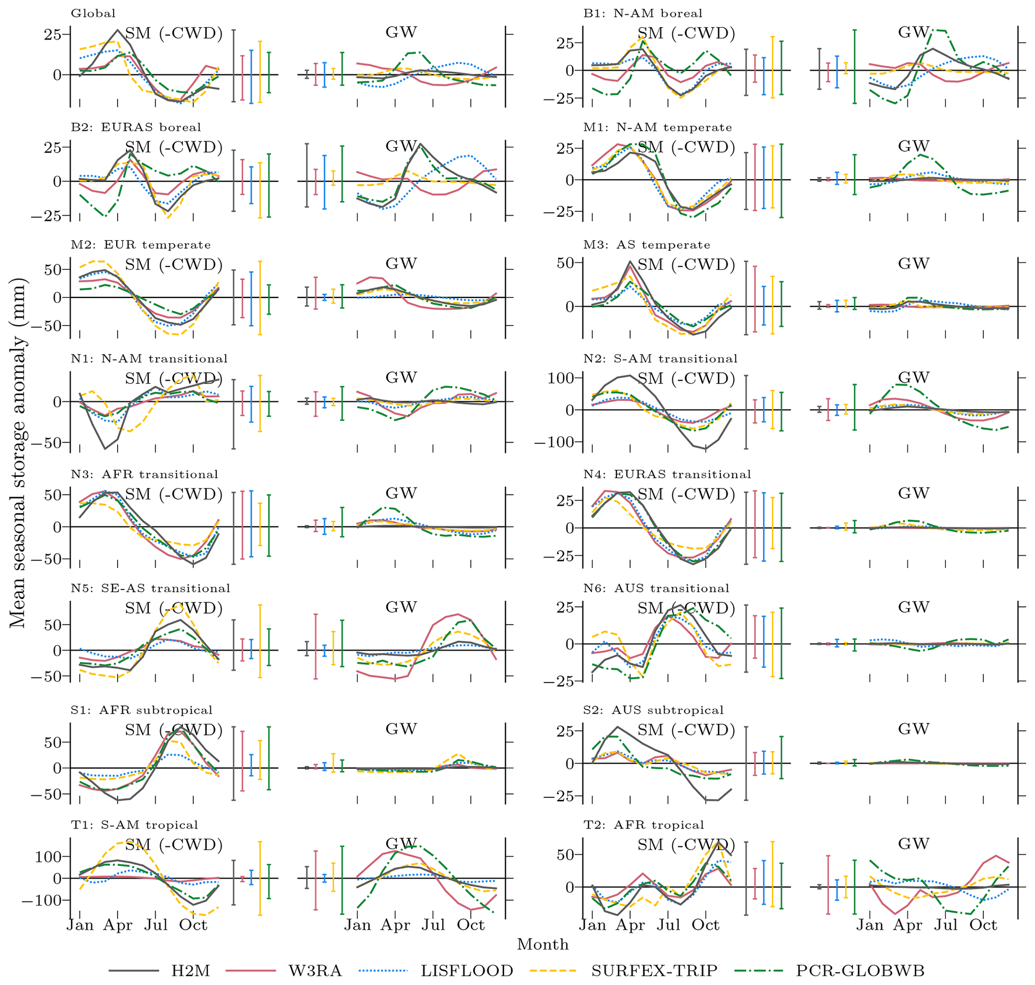
Figure B3Global and regional mean seasonal anomalies of soil moisture (SM) and groundwater (GW) for the hybrid model (H2M) and the process-based global hydrological models. Note that SM corresponds to negative modeled cumulative water deficit (CWD). Ranges from the minimum to the maximum value per model are shown next to the seasonal cycle as vertical lines. The regions are shown in Fig. 2. Surface storage is included in the groundwater component for the models SURFEX-TRIP and PCR-GLOBWB. The plots are based on global daily cell time steps from 2009 to 2014. Note that the y scale is consistent within, but differs across, regions.
The model optimization within the cross-validation setting is shown in Fig. C1. The learning process was stable in most cases, and a smooth model convergence was achieved. Only one run (fold 2; CV2) was unstable as the training collapsed. Due to the early stopping mechanism, however, the model from the best validation loss is restored and used for the test set prediction. The loss and weight (, where σ is the task uncertainty, see Sect. 2.3.3) distributions at optimum across cross-validation runs were stable (bottom row of box plots in Fig. C1). The generalization loss from the training to the validation loss is minimal, although a slightly larger spread of the validation losses can be observed. The largest generalization error occurred with SWE. Note that the training and validation sets are not only split in space but also in time. This could indicate that snow dynamics are less stable over time and change due to, for example, a warming climate.
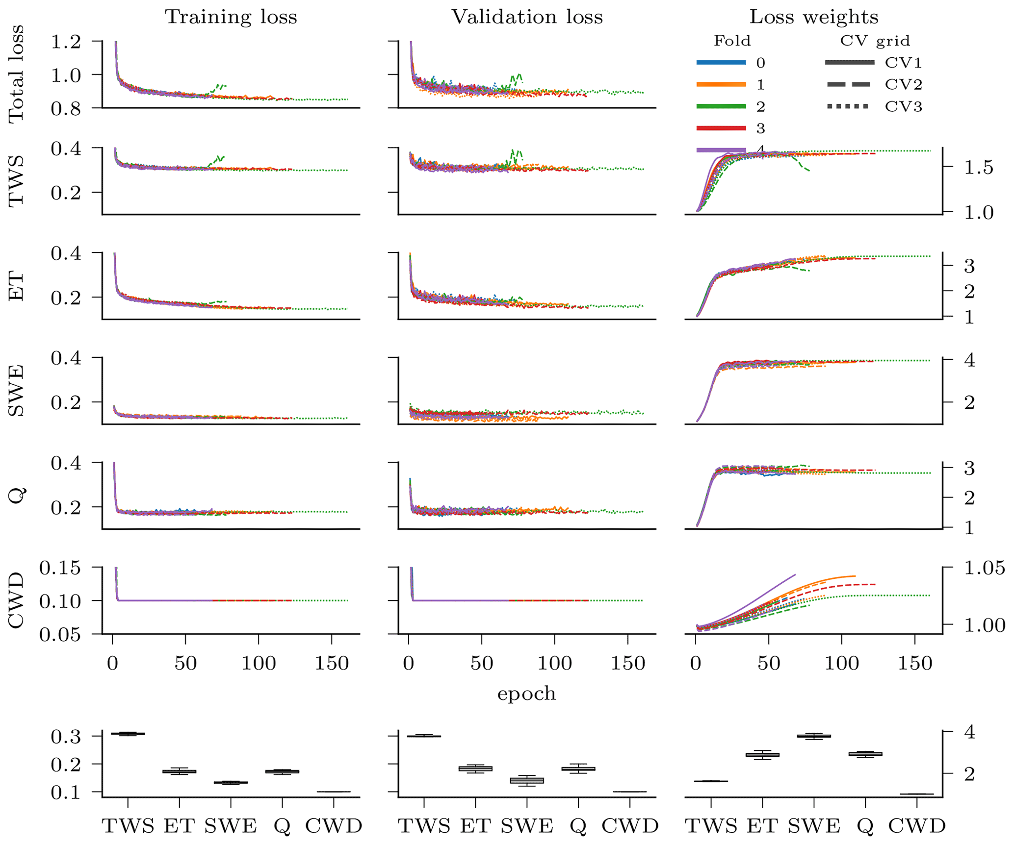
Figure C1Model training process for the cross-validation runs. The left and central columns represent the unweighted total and variable-specific mean squared error (MSE) loss. The right column shows how the task weights developed over training time. The x axis represents the number of iterations through the training set (epochs). The bottom row contains the column-wise distribution of the variables losses (or weights) at the end of the model optimization. Note that, for the soft constraint on CWD, a bias of 0.1 was added, i.e., 0.1 is the optimum.
The task weights were stable across cross-validation runs. The weights are difficult to interpret, as they do not directly translate to inverse variable uncertainty (Kendall et al., 2018) but also depend on the variable variance (although the loss is calculated on standardized data). From the box plots in Fig. C1, we can see that variables with a lower loss are given more weight, except for the CWD loss (a soft constraint that avoids CWD drift in early training), which reaches the optimum at 0.1 relatively quickly. It is possible that the lower weight of TWS is caused by its dependency on the other variables, i.e., if the model tries too hard to improve TWS, other variable losses decrease.
Part of the model tuning involved optimization of the sub-network FCNN1 (Fig. 1), extracting features from the static variables which are then fed into the recurrent neural network. We visualized the outputs (ρenc in Fig. 1) of the FCNN1 to obtain an impression of the most relevant gradients within the static variables. For visualization, the 12 activations were reduced to three dimensions using t-SNE (t-distributed stochastic neighbor embedding; Hinton and Roweis, 2002). The resulting map (Fig. C2) reveals patterns that seem very familiar, as the components align with patterns of biomass, vegetation type, and aridity. Note that the t-SNE algorithm is non-deterministic and can yield vastly different results depending on chosen hyperparameters. Also, the reduction to three dimensions only reveals the major gradients and does not represent the entire variability.
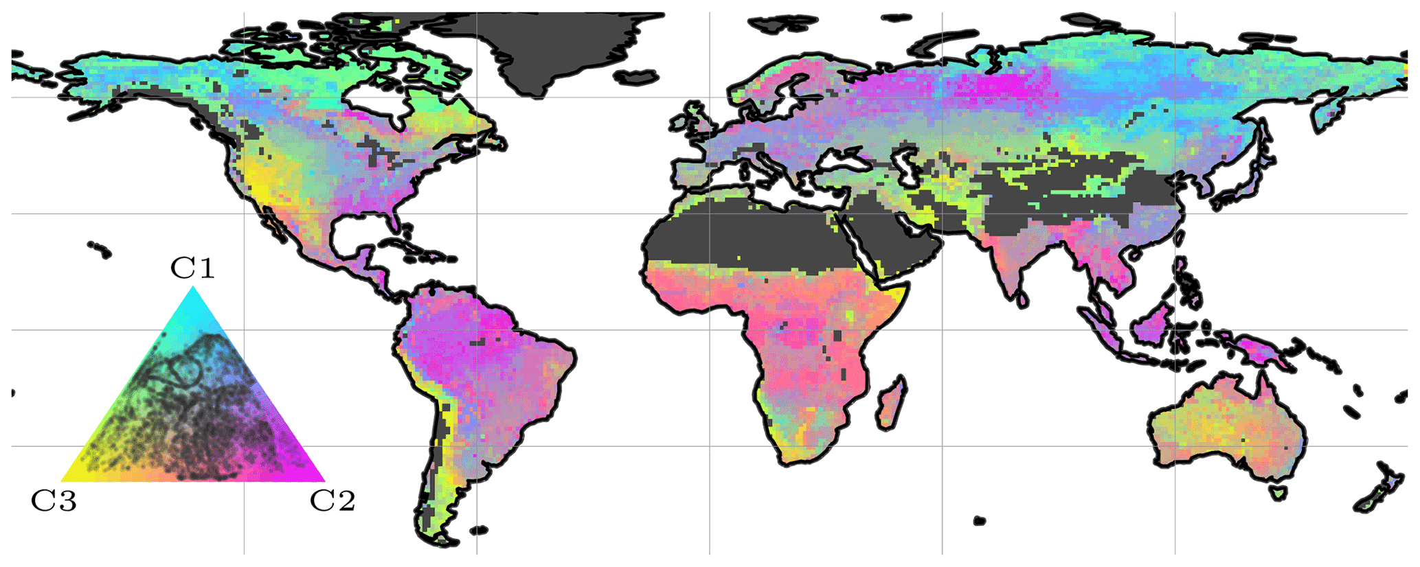
Figure C2The t-distributed stochastic neighbor (t-SNE) reduction to three dimensions (C1–3) of static variable encoding (originally 12 dimensions; ρenc in Fig. 1) of one cross-validation run. The encoding is a low-level representation of the static inputs, i.e., soil and land-cover properties, learned by a neural network. The inset ternary plots show the distribution of the map values.
To test the impact of the forcing datasets, the model was trained on the WFDEI forcings (Weedon et al., 2014) as used in the eartH2Observe ensemble. The performance (Fig. D1), with respect to TWS, was almost identical with slightly larger NSE on the global signal and lower NSE on local level when using WFDEI. The NSE of SWE was larger with WFDEI, especially for the IAV. Due to the similar performance, we conclude that the impact of the forcings is negligible, and the results are robust in regards to them.
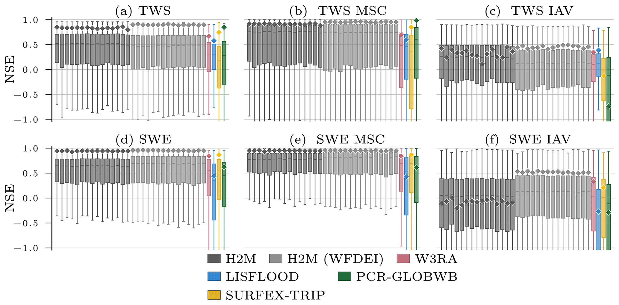
Figure D1Global and local grid cell level Nash–Sutcliffe model efficiency coefficient (NSE) of the hybrid hydrological model (H2M) and the process-based global hydrological models (GHMs) for the terrestrial water storage (TWS) on top and the snow water equivalent (SWE) at the bottom. The gray bars represent the cross-validation runs using the forcings described in Sect. 2.1.1 (dark gray; H2M), and using the WFDEI forcings as used in the eartH2Observe ensemble (light gray; H2M (WFDEI)). The ⋄ markers show the global (spatially averaged signal) model performance, and the boxes represent the spatial variability in the local cell-level performance. The y axis was cut at −1 due to some large negative NSE values. The panels show the model performance in respect to the full time series, the mean seasonal cycle (MSC), and the interannual variability (IAV). Note that, for SWE, only grid cells with at least 1 d of snow are shown, as the NSE is not defined if the observations are constant zero, which would lead to a comparison of different grid cells. The metrics are calculated from the complete common time range from 2009 to 2012 on monthly timescale. Note that deviations from the numbers reported in Table 3 are due to different time ranges.
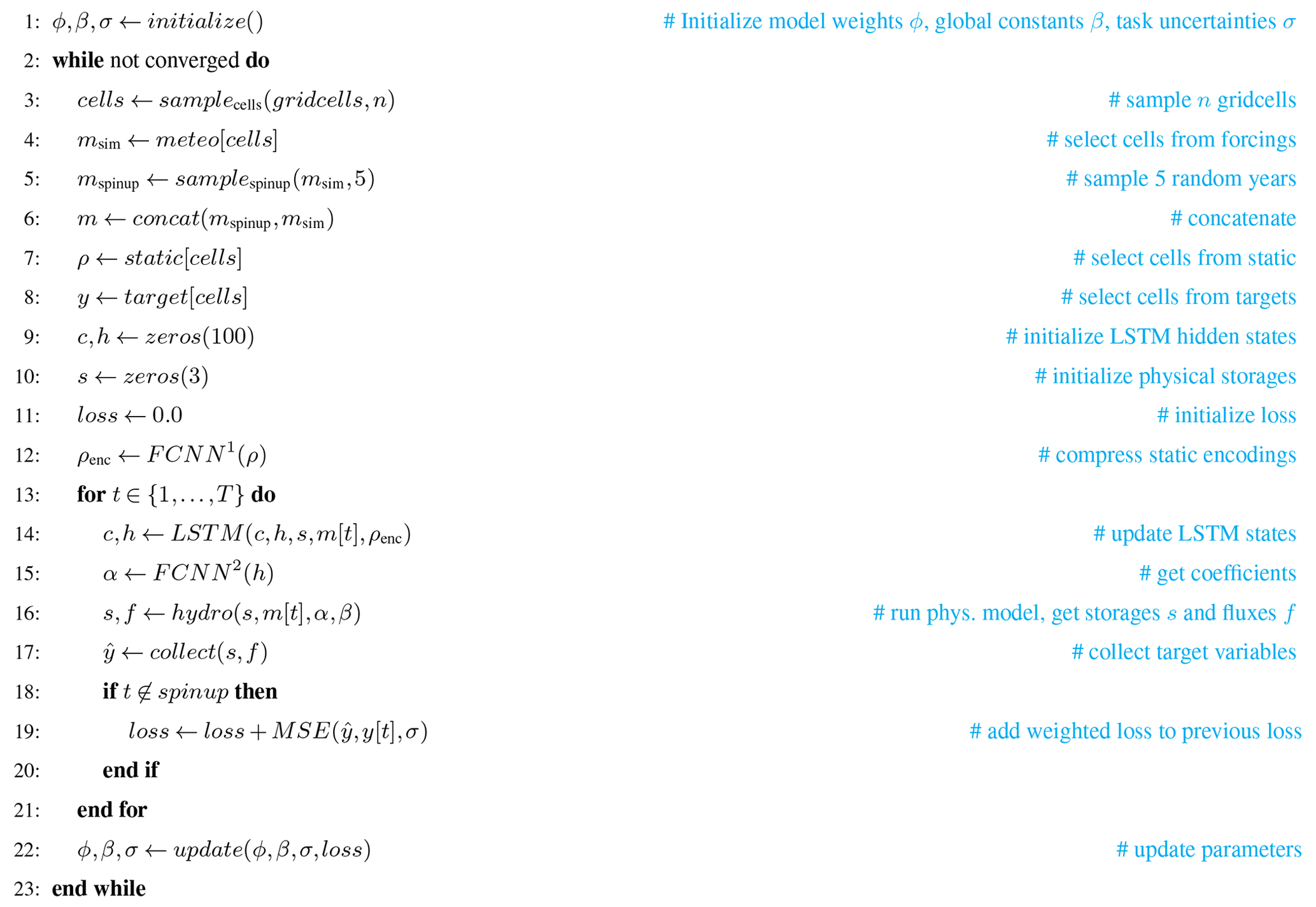
The H2M and its training are implemented in PyTorch 1.5 (Paszke et al., 2019), an open-source deep learning framework for the Python programming language (https://www.python.org/, Python Core Team, 2022). The simulated hydrological data and the code are available at https://doi.org/10.17617/3.65 (Kraft et al., 2021b). The code is also available on GitHub (https://github.com/bask0/h2m; Kraft, 2022). Note that we cannot share the data used as model input, but all datasets are referenced in the paper.
The study was conceptualized by all the authors. BK implemented the model and performed the data analysis in close collaboration with the co-authors. All authors contributed to the paper.
The contact author has declared that neither they nor their co-authors have any competing interests.
Publisher's note: Copernicus Publications remains neutral with regard to jurisdictional claims in published maps and institutional affiliations.
We thank the International Max Planck Research School for Global Biogeochemical Cycles (IMPRS-gBGC) and the Max Planck Institute for Biogeochemistry, for funding and supporting this project. In addition, we thank Uli Weber, for the data preprocessing, and our colleagues at the MPI for Biogeochemistry and TU Munich, for the stimulating discussions. We are very grateful to the reviewers Lieke Melsen, Derek Karssenberg, the anonymous referees, and Albrecht Weerts, the editor, for helping us improve the paper with their comments and suggestions.
The article processing charges for this open-access publication were covered by the Max Planck Society.
This paper was edited by Albrecht Weerts and reviewed by Derek Karssenberg and three anonymous referees.
Andrew, R., Guan, H., and Batelaan, O.: Estimation of GRACE water storage components by temporal decomposition, J. Hydrol., 552, 341–350, https://doi.org/10.1016/j.jhydrol.2017.06.016, 2017. a, b, c, d
Baldocchi, D., Falge, E., Gu, L., Olson, R., Hollinger, D., Running, S., Anthoni, P., Bernhofer, C., Davis, K., Evans, R., Fuentes, J., Goldstein, A., Katul, G., Law, B., Lee, X., Malhi, Y., Mayers, T., Munger, W., Walt, O., Paw U, K. T., Pilegaard, K., Schmid, H. P., Valentini, R., Verma, S., Vesla, T., Wilson, K., and Wofsy, S.: FLUXNET: A new tool to study the temporal and spatial variability of ecosystem-scale carbon dioxide, water vapor, and energy flux densities, B. Am. Meteorol. Soc., 82, 2415–2434, https://doi.org/10.1175/1520-0477(2001)082<2415:FANTTS>2.3.CO;2, 2001. a
Beck, H. E., van Dijk, A. I., Miralles, D. G., de Jeu, R. A., Bruijnzeel, L. S., McVicar, T. R., and Schellekens, J.: Global patterns in base flow index and recession based on streamflow observations from 3394 catchments, Water Resour. Res., 49, 7843–7863, https://doi.org/10.1002/2013WR013918, 2013. a, b
Beck, H. E., van Dijk, A. I., De Roo, A., Miralles, D. G., McVicar, T. R., Schellekens, J., and Bruijnzeel, L. A.: Global-scale regionalization of hydrologic model parameters, Water Resour. Res., 52, 3599–3622, https://doi.org/10.1002/2015WR018247, 2016. a, b, c, d
Beck, H. E., van Dijk, A. I. J. M., de Roo, A., Dutra, E., Fink, G., Orth, R., and Schellekens, J.: Global evaluation of runoff from 10 state-of-the-art hydrological models, Hydrol. Earth Syst. Sci., 21, 2881–2903, https://doi.org/10.5194/hess-21-2881-2017, 2017. a, b
Behrangi, A., Christensen, M., Richardson, M., Lebsock, M., Stephens, G., Huffman, G. J., Bolvin, D., Adler, R. F., Gardner, A., Lambrigtsen, B., and Fetzer, E.: Status of high-latitude precipitation estimates from observations and reanalyses, J. Geophys. Res.-Atmos., 121, 4468–4486, https://doi.org/10.1002/2015JD024546, 2016. a
Bergström, S.: The HBV model, in: Computer Models of Watershed Hydrology, edited by: Singh, V. P., Water Resources Publications, Colorado, USA, 443–476, ISBN 978-1887201742, 1995. a
Biancamaria, S., Lettenmaier, D. P., and Pavelsky, T. M.: The SWOT mission and its capabilities for land hydrology, Surv. Geophys., 37, 307–337, https://doi.org/10.1002/2015WR017952, 2016. a
Budyko, M. I.: Climate and life, vol. 18, Academic Press, 1 edn., ISBN 978-0121394509, 1974. a
Bui, M. T., Lu, J., and Nie, L.: A Review of Hydrological Models Applied in the Permafrost-Dominated Arctic Region, Geosciences, 10, 401, https://doi.org/10.3390/geosciences10100401, 2020. a
Chen, J., Chen, J., Liao, A., Cao, X., Chen, L., Chen, X., He, C., Han, G., Peng, S., Lu, M., Zhang, W., Tong, X., and Mills, J.: Global land cover mapping at 30 m resolution: A POK-based operational approach, ISPRS J. Photogramm., 103, 7–27, https://doi.org/10.1016/j.isprsjprs.2014.09.002, 2015. a, b
de Bézenac, E., Pajot, A., and Gallinari, P.: Deep learning for physical processes: Incorporating prior scientific knowledge, J. Stat. Mech.-Theory E., 2019, 124009, https://doi.org/10.1088/1742-5468/ab3195, 2019. a
Decharme, B. and Douville, H.: Uncertainties in the GSWP-2 precipitation forcing and their impacts on regional and global hydrological simulations, Clim. Dynam., 27, 695–713, https://doi.org/10.1007/s00382-006-0160-6, 2006. a
Decharme, B., Alkama, R., Douville, H., Becker, M., and Cazenave, A.: Global evaluation of the ISBA-TRIP continental hydrological system. Part II: Uncertainties in river routing simulation related to flow velocity and groundwater storage, J. Hydrometeorol., 11, 601–617, https://doi.org/10.1175/2010JHM1212.1, 2010. a
Decharme, B., Martin, E., and Faroux, S.: Reconciling soil thermal and hydrological lower boundary conditions in land surface models, J. Geophys. Res.-Atmos., 118, 7819–7834, https://doi.org/10.1002/jgrd.50631, 2013. a
Doelling, D.: CERES Level 3 SYN1DEG-DAYTerra+Aqua HDF4 file – Edition 4A, https://doi.org/10.5067/Terra+Aqua/CERES/SYN1degDay_L3.004A, 2017. a, b
DOI/USGS/EROS: USGS 30 ARC-second Global Elevation Data, GTOPO30, https://doi.org/10.5065/A1Z4-EE71, 1997. a, b
Döll, P. and Flörke, M.: Global-Scale estimation of diffuse groundwater recharge: model tuning to local data for semi-arid and arid regions and assessment of climate change impact, https://d-nb.info/1054768056/34 (last access: 3 March 2021), 2005. a
Falkner, S., Klein, A., and Hutter, F.: BOHB: Robust and efficient hyperparameter optimization at scale, arXiv preprint, https://arxiv.org/abs/1807.01774 (last access: 9 March 2022), 2018. a
Fan, Y., Miguez-Macho, G., Jobbágy, E. G., Jackson, R. B., and Otero-Casal, C.: Hydrologic regulation of plant rooting depth, P. Natl. Acad. Sci. USA, 114, 10572–10577, https://doi.org/10.1073/pnas.1712381114, 2017. a
Feddema, J. J.: A revised Thornthwaite-type global climate classification, Phys. Geogr., 26, 442–466, https://doi.org/10.2747/0272-3646.26.6.442, 2005. a
Fekete, B. M., Vörösmarty, C. J., and Grabs, W.: Global, composite runoff fields based on observed river discharge and simulated water balances, https://csdms.colorado.edu/wiki/Data:GRDC (last access: 9 March 2022), Global Runoff Data Centre Koblenz [data], 1999. a
Geer, A.: Learning earth system models from observations: machine learning or data assimilation?, Philos. T. Roy. Soc. A, 379, 20200089, https://doi.org/10.1098/rsta.2020.0089, 2021. a, b
Geirhos, R., Jacobsen, J.-H., Michaelis, C., Zemel, R., Brendel, W., Bethge, M., and Wichmann, F. A.: Shortcut learning in deep neural networks, Nature Machine Intelligence, 2, 665–673, https://doi.org/10.1038/s42256-020-00257-z, 2020. a
Getirana, A., Kumar, S., Girotto, M., and Rodell, M.: Rivers and floodplains as key components of global terrestrial water storage variability, Geophys. Res. Lett., 44, 10–359, https://doi.org/10.1002/2017GL074684, 2017. a
Ghiggi, G., Humphrey, V., Seneviratne, S. I., and Gudmundsson, L.: GRUN: an observation-based global gridded runoff dataset from 1902 to 2014, Earth Syst. Sci. Data, 11, 1655–1674, https://doi.org/10.5194/essd-11-1655-2019, 2019. a, b, c
Goodfellow, I., Bengio, Y., and Courville, A.: Deep Learning, MIT press, http://www.deeplearningbook.org (last access: 9 March 2022), ISBN 9780262035613, 2016. a, b, c, d
Grayson, R. B., Andrew, W., Walker, J. P., Kandel, D. G., Costelloe, J. F., and Wilson, D. J.: Controls on patterns of soil moisture in arid and semi-arid systems, in: Dryland ecohydrology, edited by: D'Odorico, P. and Porporato, A., Springer, Dordrecht, the Netherlands, 109–127, https://doi.org/10.1007/1-4020-4260-4_7, 2006. a
Güntner, A.: Improvement of global hydrological models using GRACE data, Surv. Geophys., 29, 375–397, https://doi.org/10.1007/s10712-008-9038-y, 2008. a
Güntner, A., Stuck, J., Werth, S., Döll, P., Verzano, K., and Merz, B.: A global analysis of temporal and spatial variations in continental water storage, Water Resour. Res., 43, W05416, https://doi.org/10.1029/2006WR005247, 2007. a, b
Haddeland, I., Clark, D. B., Franssen, W., Ludwig, F., Voß, F., Arnell, N. W., Bertrand, N., Best, M., Folwell, S., Gerten, D., Gomes, S., Gosling, S. N., Hagemann, S., Hanasaki, N., Harding, R., Heinke, J., Kabat, P., Koirala, Sujan amd Oki, T., Polcher, J., Stacke, T., Viterbo, P., Weedon, G. P., and Yeh, P.: Multimodel estimate of the global terrestrial water balance: setup and first results, J. Hydrometeorol., 12, 869–884, https://doi.org/10.1175/2011JHM1324.1, 2011. a
Hall, D. and Riggs, G.: Modis/Terra Snow Cover 8-Day L3 Global 0.05 Deg CMG, https://doi.org/10.5067/MODIS/MOD10C2.006, 2016. a
Harris, I., Jones, P. D., Osborn, T. J., and Lister, D. H.: Updated high-resolution grids of monthly climatic observations–the CRU TS3. 10 Dataset, Int. J. Climatol., 34, 623–642, https://doi.org/10.1002/joc.3711, 2014. a, b
Hengl, T., de Jesus, J. M., Heuvelink, G. B., Gonzalez, M. R., Kilibarda, M., Blagotić, A., Shangguan, W., Wright, M. N., Geng, X., Bauer-Marschallinger, B., Guevara, M. A., Vargas, R., MacMillan, R. A., Batjes, N. H., Leenaars, J. G. B., Ribeiro, E., Wheeler, I., Mantel, S., and Kempen, B.: SoilGrids250m: Global gridded soil information based on machine learning, PLoS ONE, 12, e0169748, https://doi.org/10.1371/journal.pone.0169748, 2017. a, b, c
Hinton, G. and Roweis, S. T.: Stochastic neighbor embedding, in: NIPS, vol. 15, Citeseer, 833–840, http://papers.nips.cc/paper/2276-stochastic-neighbor-embedding (last access: 9 March 2022), 2002. a
Hochreiter, S. and Schmidhuber, J.: Long short-term memory, Neural Comput., 9, 1735–1780, https://doi.org/10.1162/neco.1997.9.8.1735, 1997. a
Huffman, G., Bolvin, D., and Adler, R.: GPCP version 1.2 1-degree daily (1DD) precipitation data set, World Data Center A, National Climatic Data Center, Asheville, NC, https://doi.org/10.5065/d6d50k46, 2012. a, b
Humphrey, V., Gudmundsson, L., and Seneviratne, S. I.: Assessing global water storage variability from GRACE: trends, seasonal cycle, subseasonal anomalies and extremes, Surv. Geophys., 37, 357–395, https://doi.org/10.1007/s10712-016-9367-1, 2016. a, b, c
Ichii, K., Wang, W., Hashimoto, H., Yang, F., Votava, P., Michaelis, A. R., and Nemani, R. R.: Refinement of rooting depths using satellite-based evapotranspiration seasonality for ecosystem modeling in California, Agric. Forest Meteorol., 149, 1907–1918, https://doi.org/10.1016/j.agrformet.2009.06.019, 2009. a
Jackson, R. B., Schenk, H., Jobbagy, E., Canadell, J., Colello, G., Dickinson, R., Field, C., Friedlingstein, P., Heimann, M., Hibbard, K., Kicklighter, D. W., Kleidon, A., Neilson, R. P., Parton, W. J., Sala, O. E., and Sykes, M. T.: Belowground consequences of vegetation change and their treatment in models, Ecol. Appl., 10, 470–483, https://doi.org/10.1890/1051-0761(2000)010[0470:BCOVCA]2.0.CO;2, 2000. a
Jasechko, S., Birks, S. J., Gleeson, T., Wada, Y., Fawcett, P. J., Sharp, Z. D., McDonnell, J. J., and Welker, J. M.: The pronounced seasonality of global groundwater recharge, Water Resour. Res., 50, 8845–8867, https://doi.org/10.1002/2014WR015809, 2014. a
Jiménez Cisneros, B. E., Oki, T., Arnell, N. W., Benito, G., Cogley, J. G., Döll, P., Jiang, T., Mwakalila, S. S., Fischer, T., Gerten, D., Hock, R., Kanae, S., Lu, X., Mata, L. J., Pahl-Wostl, C., Strzepek, K. M., Su, B., and van den Hurk, B.: Freshwater resources, in: Climate change 2014: impacts, adaptation, and vulnerability. Part A: global and sectoral aspects. Contribution of working group II to the fifth assessment report of the intergovernmental panel on climate change, edited by: Field, C. B., Cambridge University Press, 229–269, https://doi.org/10.1017/CBO9781107415379.008, 2014. a
Jung, M., Reichstein, M., Schwalm, C. R., Huntingford, C., Sitch, S., Ahlström, A., Arneth, A., Camps-Valls, G., Ciais, P., Friedlingstein, P., Gans, F., Ichii, K., Jain, A. K., Kato, E., Papale, D., Poulter, B., Raduly, B., Rödenbeck, C., Tramontana, G., Viovy, N., Wang, Y.-P., Weber, U., Zaehle, S., and Zeng, N.: Compensatory water effects link yearly global land CO2 sink changes to temperature, Nature, 541, 516–520, https://doi.org/10.1038/nature20780, 2017. a, b
Jung, M., Koirala, S., Weber, U., Ichii, K., Gans, F., Camps-Valls, G., Papale, D., Schwalm, C., Tramontana, G., and Reichstein, M.: The FLUXCOM ensemble of global land-atmosphere energy fluxes, Scientific Data, 6, 1–14, https://doi.org/10.1038/s41597-019-0076-8, 2019. a, b
Jung, M., Schwalm, C., Migliavacca, M., Walther, S., Camps-Valls, G., Koirala, S., Anthoni, P., Besnard, S., Bodesheim, P., Carvalhais, N., Chevallier, F., Gans, F., Goll, D. S., Haverd, V., Köhler, P., Ichii, K., Jain, A. K., Liu, J., Lombardozzi, D., Nabel, J. E. M. S., Nelson, J. A., O'Sullivan, M., Pallandt, M., Papale, D., Peters, W., Pongratz, J., Rödenbeck, C., Sitch, S., Tramontana, G., Walker, A., Weber, U., and Reichstein, M.: Scaling carbon fluxes from eddy covariance sites to globe: synthesis and evaluation of the FLUXCOM approach, Biogeosciences, 17, 1343–1365, https://doi.org/10.5194/bg-17-1343-2020, 2020. a
Kendall, A., Gal, Y., and Cipolla, R.: Multi-Task Learning Using Uncertainty to Weigh Losses for Scene Geometry and Semantics, in: IEEE Conference on Computer Vision and Pattern Recognition (CVPR), pp. 7482–7491, https://doi.org/10.1109/CVPR.2018.00781, Salt Lake City, UT, USA, 18–22 June 2018. a, b
Kim, H., Yeh, P. J.-F., Oki, T., and Kanae, S.: Role of rivers in the seasonal variations of terrestrial water storage over global basins, Geophys. Res. Lett., 36, L17402, https://doi.org/10.1029/2009GL039006, 2009. a, b
Kleidon, A. and Heimann, M.: Assessing the role of deep rooted vegetation in the climate system with model simulations: mechanism, comparison to observations and implications for Amazonian deforestation, Clim. Dynam., 16, 183–199, https://doi.org/10.1007/s003820050012, 2000. a
Koirala, S., Jung, M., Reichstein, M., de Graaf, I. E., Camps-Valls, G., Ichii, K., Papale, D., Ráduly, B., Schwalm, C. R., Tramontana, G., and Carvalhais, N.: Global distribution of groundwater-vegetation spatial covariation, Geophys. Res. Lett., 44, 4134–4142, https://doi.org/10.1002/2017GL072885, 2017. a, b
Körner, M. and Rußwurm, M.: Recurrent Neural Networks and the Temporal Component, in: Deep Learning for the Earth Sciences: A Comprehensive Approach to Remote Sensing, Climate Science and Geosciences, edited by: Camps-Valls, G., Tuia, D., Zhu, X. X., and Reichstein, M., pp. 105–119, Wiley & Sons, 1st edn., ISBN 978-1-119-64614-3, 2021. a
Kraft, B.: H2M model code, GitHub [code], https://github.com/bask0/h2m, last access: 21 March 2021. a
Kraft, B., Jung, M., Körner, M., Requena Mesa, C., Cortés, J., and Reichstein, M.: Identifying dynamic memory effects on vegetation state using recurrent neural networks, Frontiers in Big Data, 2, 31, https://doi.org/10.3389/fdata.2019.00031, 2019. a
Kraft, B., Jung, M., Körner, M., and Reichstein, M.: Hybrid modeling: Fusion of a deep learning approach and a physics-based model for global hydrological modeling, Int. Arch. Photogramm., 43, 1537–1544, https://doi.org/10.5194/isprs-archives-XLIII-B2-2020-1537-2020, 2020. a, b, c, d
Kraft, B., Besnard, S., and Koirala, S.: Emulating Ecological Memory with Recurrent Neural Networks, Deep Learning for the Earth Sciences: A Comprehensive Approach to Remote Sensing, Climate Science, and Geosciences, 269–281, Wiley & Sons, ISBN 978-1-119-64614-3, https://doi.org/10.1002/9781119646181.ch18, 2021a. a
Kraft, B., Jung, M., Körner, M., Koirala, S., and Reichstein, M.: Daily model simulations, Edmond [data set], https://doi.org/10.17617/3.65, 2021b. a
Kumar, A.: Stage-Discharge Relationship, in: Encyclopedia of Snow, Ice and Glaciers. Encyclopedia of Earth Sciences Series, edited by: Singh, V., Singh, P., and Haritashya, U., Springer, Dordrecht, https://doi.org/10.1007/978-90-481-2642-2_537, 2011. a
Kvas, A., Behzadpour, S., Ellmer, M., Klinger, B., Strasser, S., Zehentner, N., and Mayer-Gürr, T.: ITSG-Grace2018: Overview and evaluation of a new GRACE-only gravity field time series, J. Geophys. Res.-Sol. Ea., 124, 9332–9344, https://doi.org/10.1029/2019JB017415, 2019. a
Liaw, R., Liang, E., Nishihara, R., Moritz, P., Gonzalez, J. E., and Stoica, I.: Tune: A research platform for distributed model selection and training, arXiv preprint, https://arxiv.org/abs/1807.05118 (last access: 9 March 2022), 2018. a
Loshchilov, I. and Hutter, F.: Decoupled weight decay regularization, arXiv preprint, https://arxiv.org/abs/1711.05101v3 (last access: 9 March 2022), 2017. a, b
Luojus, K., Pulliainen, J., Takala, M., Derksen, C., Rott, H., Nagler, T., Solberg, R., Wiesmann, A., Metsamaki, S., Malnes, E., and Bojkov, B.: Investigating the feasibility of the GlobSnow snow water equivalent data for climate research purposes, in: 2010 IEEE International Geoscience and Remote Sensing Symposium, pp. 4851–4853, IEEE, Honolulu, HI, USA, https://doi.org/10.1109/IGARSS.2010.5741987, 2010. a
Luojus, K., Pulliainen, J., Takala, M., Lemmetyinen, J., Kangwa, M., Eskelinen, M., Metsämäki, S., Solberg, R., Salberg, A.-B., Bippus, G., Ripper, E., Nagler, T., Derksen, C., Wiesmann, A., Wunderle, S., Hüsler, F., Fontana, F., and Foppa, N.: GlobSnow-2 Final Report – European space agency study contract report, http://www.globsnow.info/docs/GlobSnow_2_Final_Report_release.pdf (last access: 3 March 2021), 2014. a, b
McLaughlin, D.: An integrated approach to hydrologic data assimilation: interpolation, smoothing, and filtering, Adv. Water Resour., 25, 1275–1286, https://doi.org/10.1016/S0309-1708(02)00055-6, 2002. a
Moradkhani, H., Sorooshian, S., Gupta, H. V., and Houser, P. R.: Dual state–parameter estimation of hydrological models using ensemble Kalman filter, Adv. Water Resour., 28, 135–147, https://doi.org/10.1016/j.advwatres.2004.09.002, 2005. a, b
Nash, J. E. and Sutcliffe, J. V.: River flow forecasting through conceptual models part I – A discussion of principles, J. Hydrol., 10, 282–290, https://doi.org/10.1016/0022-1694(70)90255-6, 1970. a
Nicholson, S. E.: Dryland Climatology, Cambridge University Press, Cambridge, UK, https://doi.org/10.1017/CBO9780511973840, 2011. a
Pachauri, R. K., Allen, M. R., Barros, V. R., Broome, J., Cramer, W., Christ, R., Church, J. A., Clarke, L., Dahe, Q., Dasgupta, P., Dubash, N. K., Edenhofer, O., Elgizouli, I., Field, C. B., Forster, P., Friedlingstein, P., Fuglestvedt, J., Gomez-Echeverri, L., Hallegatte, S., Hegerl, G., Howden, M., Jiang, K., Jimenez Cisneroz, B., Kattsov, V., Lee, H., Mach, K. J., Marotzke, J., Mastrandrea, M. D., Meyer, L., Minx, J., Mulugetta, Y., O'Brien, K., Oppenheimer, M., Pereira, J. J., Pichs-Madruga, R., Plattner, G.-K., Pörtner, H.-O., Power, S. B., Preston, B., Ravindranath, N. H., Reisinger, A., Riahi, K., Rusticucci, M., Scholes, R., Seyboth, K., Sokona, Y., Stavins, R., Stocker, T. F., Tschakert, P., van Vuuren, D., and van Ypserle, J.-P.: Climate change 2014: synthesis report. Contribution of Working Groups I, II and III to the fifth assessment report of the Intergovernmental Panel on Climate Change, IPCC, ISBN 978-92-9169-143-2, 2014. a
Panahi, M. and Behrangi, A.: Comparative analysis of snowfall accumulation and gauge undercatch correction factors from diverse data sets: In situ, satellite, and reanalysis, Asia-Pac. J. Atmos. Sci., 56, 1–14, https://doi.org/10.1007/s13143-019-00161-6, 2019. a
Papagiannopoulou, C., Miralles, D. G., Demuzere, M., Verhoest, N. E. C., and Waegeman, W.: Global hydro-climatic biomes identified via multitask learning, Geosci. Model Dev., 11, 4139–4153, https://doi.org/10.5194/gmd-11-4139-2018, 2018. a, b
Paszke, A., Gross, S., Massa, F., Lerer, A., Bradbury, J., Chanan, G., Killeen, T., Lin, Z., Gimelshein, N., Antiga, L., Desmaison, A., Kopf, A., Yang, E., DeVito, Z., Raison, M., Tejani, A., Chilamkurthy, S., Steiner, B., Fang, L., Bai, J., and Chintala, S.: PyTorch: An Imperative Style, High-Performance Deep Learning Library, in: Advances in Neural Information Processing Systems, vol. 32, Curran Associates, Inc., https://proceedings.neurips.cc/paper/2019/file/bdbca288fee7f92f2bfa9f7012727740-Paper.pdf (last access: 9 March 2022), 2019. a
Python Core Team: Python: A dynamic, open source programming language, Python Software Foundation, https://www.python.org/, 9 March 2022. a
Rangelova, E., Van der Wal, W., Braun, A., Sideris, M., and Wu, P.: Analysis of Gravity Recovery and Climate Experiment time-variable mass redistribution signals over North America by means of principal component analysis, J. Geophys. Res.-Earth, 112, F03002, https://doi.org/10.1029/2006JF000615, 2007. a
Rasp, S., Pritchard, M. S., and Gentine, P.: Deep learning to represent subgrid processes in climate models, P. Natl. Acad. Sci. USA, 115, 9684–9689, https://doi.org/10.1073/pnas.1810286115, 2018. a
Reichle, R. H.: Data assimilation methods in the Earth sciences, Adv. Water Resour., 31, 1411–1418, https://doi.org/10.1016/j.advwatres.2008.01.001, 2008. a, b
Reichstein, M., Camps-Valls, G., Stevens, B., Jung, M., Denzler, J., Carvalhais, N., and Prabhat: Deep learning and process understanding for data-driven Earth system science, Nature, 566, 195, https://doi.org/10.1038/s41586-019-0912-1, 2019. a
Roberts, D. R., Bahn, V., Ciuti, S., Boyce, M. S., Elith, J., Guillera-Arroita, G., Hauenstein, S., Lahoz-Monfort, J. J., Schröder, B., Thuiller, W., Warton, D. I., Wintle, B. A., Hartig, F., and Dormann, C. F.: Cross-validation strategies for data with temporal, spatial, hierarchical, or phylogenetic structure, Ecography, 40, 913–929, https://doi.org/10.1111/ecog.02881, 2017. a
Rodell, M., Famiglietti, J., Wiese, D., Reager, J., Beaudoing, H., Landerer, F. W., and Lo, M.-H.: Emerging trends in global freshwater availability, Nature, 557, 651–659, https://doi.org/10.1038/s41586-018-0123-1, 2018. a, b
Scanlon, B. R., Zhang, Z., Rateb, A., Sun, A., Wiese, D., Save, H., Beaudoing, H., Lo, M. H., Müller-Schmied, H., Döll, P., van Beek, R., Swenson, S., Lawrence, D., Croteau, M., and Reedy, R. C.: Tracking seasonal fluctuations in land water storage using global models and GRACE satellites, Geophys. Res. Lett., 46, 5254–5264, https://doi.org/10.1029/2018GL081836, 2019. a, b, c, d
Scanlon, B. R., Zhang, Z., Save, H., Wiese, D. N., Landerer, F. W., Long, D., Longuevergne, L., and Chen, J.: Global evaluation of new GRACE mascon products for hydrologic applications, Water Resour. Res., 52, 9412–9429, https://doi.org/10.1002/2016WR019494, 2016. a
Schellekens, J., Dutra, E., Martínez-de la Torre, A., Balsamo, G., van Dijk, A., Sperna Weiland, F., Minvielle, M., Calvet, J.-C., Decharme, B., Eisner, S., Fink, G., Flörke, M., Peßenteiner, S., van Beek, R., Polcher, J., Beck, H., Orth, R., Calton, B., Burke, S., Dorigo, W., and Weedon, G. P.: A global water resources ensemble of hydrological models: the eartH2Observe Tier-1 dataset, Earth Syst. Sci. Data, 9, 389–413, https://doi.org/10.5194/essd-9-389-2017, 2017. a, b, c, d, e
Schwingshackl, C., Hirschi, M., and Seneviratne, S. I.: Quantifying spatiotemporal variations of soil moisture control on surface energy balance and near-surface air temperature, J. Climate, 30, 7105–7124, https://doi.org/10.1175/JCLI-D-16-0727.1, 2017. a
Seneviratne, S. I., Corti, T., Davin, E. L., Hirschi, M., Jaeger, E. B., Lehner, I., Orlowsky, B., and Teuling, A. J.: Investigating soil moisture–climate interactions in a changing climate: A review, Earth-Sci. Rev., 99, 125–161, https://doi.org/10.1016/j.earscirev.2010.02.004, 2010. a
Shen, C., Laloy, E., Elshorbagy, A., Albert, A., Bales, J., Chang, F.-J., Ganguly, S., Hsu, K.-L., Kifer, D., Fang, Z., Fang, K., Li, D., Li, X., and Tsai, W.-P.: HESS Opinions: Incubating deep-learning-powered hydrologic science advances as a community, Hydrol. Earth Syst. Sci., 22, 5639–5656, https://doi.org/10.5194/hess-22-5639-2018, 2018. a
Sun, L., Seidou, O., Nistor, I., and Liu, K.: Review of the Kalman-type hydrological data assimilation, Hydrolog. Sci. J., 61, 2348–2366, https://doi.org/10.1080/02626667.2015.1127376, 2016. a
Swenson, S., Famiglietti, J., Basara, J., and Wahr, J.: Estimating profile soil moisture and groundwater variations using GRACE and Oklahoma Mesonet soil moisture data, Water Resour. Res., 44, W01413, https://doi.org/10.1029/2007WR006057, 2008. a
Sylla, M., Giorgi, F., Coppola, E., and Mariotti, L.: Uncertainties in daily rainfall over Africa: assessment of gridded observation products and evaluation of a regional climate model simulation, Int. J. Climatol., 33, 1805–1817, https://doi.org/10.1002/joc.3551, 2013. a
Takala, M., Luojus, K., Pulliainen, J., Derksen, C., Lemmetyinen, J., Kärnä, J.-P., Koskinen, J., and Bojkov, B.: Estimating northern hemisphere snow water equivalent for climate research through assimilation of space-borne radiometer data and ground-based measurements, Remote Sens. Environ., 115, 3517–3529, https://doi.org/10.1016/j.rse.2011.08.014, 2011. a, b
Taylor, K. E., Stouffer, R. J., and Meehl, G. A.: An overview of CMIP5 and the experiment design, B. Am. Meteorol. Soc., 93, 485–498, https://doi.org/10.1175/BAMS-D-11-00094.1, 2012. a
Tootchi, A., Jost, A., and Ducharne, A.: Multi-source global wetland maps combining surface water imagery and groundwater constraints, Earth Syst. Sci. Data, 11, 189–220, https://doi.org/10.5194/essd-11-189-2019, 2019. a, b
Tramontana, G., Jung, M., Schwalm, C. R., Ichii, K., Camps-Valls, G., Ráduly, B., Reichstein, M., Arain, M. A., Cescatti, A., Kiely, G., Merbold, L., Serrano-Ortiz, P., Sickert, S., Wolf, S., and Papale, D.: Predicting carbon dioxide and energy fluxes across global FLUXNET sites with regression algorithms, Biogeosciences, 13, 4291–4313, https://doi.org/10.5194/bg-13-4291-2016, 2016. a, b
Trautmann, T., Koirala, S., Carvalhais, N., Eicker, A., Fink, M., Niemann, C., and Jung, M.: Understanding terrestrial water storage variations in northern latitudes across scales, Hydrol. Earth Syst. Sci., 22, 4061–4082, https://doi.org/10.5194/hess-22-4061-2018, 2018. a, b, c
Trautmann, T., Koirala, S., Carvalhais, N., Güntner, A., and Jung, M.: The importance of vegetation in understanding terrestrial water storage variations, Hydrol. Earth Syst. Sci., 26, 1089–1109, https://doi.org/10.5194/hess-26-1089-2022, 2022. a
Van Beek, L., Wada, Y., and Bierkens, M. F.: Global monthly water stress: 1. Water balance and water availability, Water Resour. Res., 47, W07517, https://doi.org/10.1029/2010WR009792, 2011. a, b
Van Der Knijff, J., Younis, J., and De Roo, A.: LISFLOOD: a GIS-based distributed model for river basin scale water balance and flood simulation, Int. J. Geogr. Inf. Sci., 24, 189–212, https://doi.org/10.1080/13658810802549154, 2010. a, b
Van Dijk, A. and Warren, G.: The Australian water resources assess- ment system, version 0.5, 3, http://www.clw.csiro.au/publications/waterforahealthycountry/2010/wfhc-awras-evaluation-against-observations.pdf (last access: 3 March 2021), 2010. a
van Dijk, A. I. J. M., Renzullo, L. J., Wada, Y., and Tregoning, P.: A global water cycle reanalysis (2003–2012) merging satellite gravimetry and altimetry observations with a hydrological multi-model ensemble, Hydrol. Earth Syst. Sci., 18, 2955–2973, https://doi.org/10.5194/hess-18-2955-2014, 2014. a
Viovy, N.: CRUNCEP version 7-atmospheric forcing data for the community land model, Research Data Archive at the National Center for Atmospheric Research, Computational and Information Systems Laboratory, Boulder CO, USA, https://doi.org/10.5065/PZ8F-F017, 2018. a, b
Wada, Y., Wisser, D., and Bierkens, M. F. P.: Global modeling of withdrawal, allocation and consumptive use of surface water and groundwater resources, Earth Syst. Dynam., 5, 15–40, https://doi.org/10.5194/esd-5-15-2014, 2014. a
Wang, H. and Yeung, D.-Y.: A survey on Bayesian deep learning, ACM Comput. Surv., 53, 1–37, https://doi.org/10.1145/3409383, 2020. a
Watkins, M. M., Wiese, D. N., Yuan, D.-N., Boening, C., and Landerer, F. W.: Improved methods for observing Earth's time variable mass distribution with GRACE using spherical cap mascons, J. Geophys. Res.-Sol. Ea., 120, 2648–2671, https://doi.org/10.1002/2014JB011547, 2015. a, b
Weedon, G. P., Balsamo, G., Bellouin, N., Gomes, S., Best, M. J., and Viterbo, P.: The WFDEI meteorological forcing data set: WATCH Forcing Data methodology applied to ERA-Interim reanalysis data, Water Resour. Res., 50, 7505–7514, https://doi.org/10.1002/2014WR015638, 2014. a, b
Wielicki, B. A., Barkstrom, B. R., Harrison, E. F., Lee III, R. B., Smith, G. L., and Cooper, J. E.: Clouds and the Earth's Radiant Energy System (CERES): An Earth Observing System Experiment, B. Am. Meteorol. Soc., 77, 853–868, https://doi.org/10.1175/1520-0477(1996)077<0853:CATERE>2.0.CO;2, 1996. a, b
Wiese, D. N., Landerer, F. W., and Watkins, M. M.: Quantifying and reducing leakage errors in the JPL RL05M GRACE mascon solution, Water Resour. Res., 52, 7490–7502, https://doi.org/10.1002/2016WR019344, 2016. a
Wiese, D. N., Yuan, D.-N., Boening, C., Landerer, F. W., and Watkins, M. M.: JPL GRACE Mascon Ocean, Ice, and Hydrology Equivalent Water Height Release 06 Coastal Resolution Improvement (CRI) Filtered, PO.DAAC, CA, USA, https://doi.org/10.5067/TEMSC-3MJC6, 2018. a, b
Yang, Y., Donohue, R. J., and McVicar, T. R.: Global estimation of effective plant rooting depth: Implications for hydrological modeling, Water Resour. Res., 52, 8260–8276, https://doi.org/10.1002/2016WR019392, 2016. a, b
Zelazowski, P., Malhi, Y., Huntingford, C., Sitch, S., and Fisher, J. B.: Changes in the potential distribution of humid tropical forests on a warmer planet, Philos. T. Roy. Soc. A, 369, 137–160, https://doi.org/10.1098/rsta.2010.0238, 2011. a
Zeng, N., Yoon, J.-H., Mariotti, A., and Swenson, S.: Variability of basin-scale terrestrial water storage from a PER water budget method: The Amazon and the Mississippi, J. Climate, 21, 248–265, https://doi.org/10.1175/2007JCLI1639.1, 2008. a, b
- Abstract
- Introduction
- Data and methods
- Results
- Discussion
- Conclusions
- Appendix A: Spatial model performance
- Appendix B: Regional comparison of simulated time series
- Appendix C: Model optimization
- Appendix D: Model forcing with WFDEI
- Appendix E: Model pseudocode
- Code and data availability
- Author contributions
- Competing interests
- Disclaimer
- Acknowledgements
- Financial support
- Review statement
- References