A space–time Bayesian hierarchical modeling framework for projection of seasonal maximum streamflow

Timely projections of seasonal streamflow extremes can be useful for the early implementation of annual flood risk adaptation strategies. However, predicting seasonal extremes is challenging, particularly under nonstationary conditions and if extremes are correlated in space. The goal of this study is to implement a space–time model for the projection of seasonal streamflow extremes that considers the nonstationarity (interannual variability) and spatiotemporal dependence of high flows. We develop a space–time model to project seasonal streamflow extremes for several lead times up to 2 months, using a Bayesian hierarchical modeling (BHM) framework. This model is based on the assumption that streamflow extremes (3 d maxima) at a set of gauge locations are realizations of a Gaussian elliptical copula and generalized extreme value (GEV) margins with nonstationary parameters. These parameters are modeled as a linear function of suitable covariates describing the previous season selected using the deviance information criterion (DIC). Finally, the copula is used to generate streamflow ensembles, which capture spatiotemporal variability and uncertainty. We apply this modeling framework to predict 3 d maximum streamflow in spring (May–June) at seven gauges in the Upper Colorado River basin (UCRB) with 0- to 2-month lead time. In this basin, almost all extremes that cause severe flooding occur in spring as a result of snowmelt and precipitation. Therefore, we use regional mean snow water equivalent and temperature from the preceding winter season as well as indices of large-scale climate teleconnections – El Niño–Southern Oscillation, Atlantic Multidecadal Oscillation, and Pacific Decadal Oscillation – as potential covariates for 3 d spring maximum streamflow. Our model evaluation, which is based on the comparison of different model versions and the energy skill score, indicates that the model can capture the space–time variability in extreme streamflow well and that model skill increases with decreasing lead time. We also find that the use of climate variables slightly enhances skill relative to using only snow information. Median projections and their uncertainties are consistent with observations, thanks to the representation of spatial dependencies through covariates in the margins and a Gaussian copula. This spatiotemporal modeling framework helps in the planning of seasonal adaptation and preparedness measures as predictions of extreme spring streamflows become available 2 months before actual flood occurrence.

1 Introduction

Floods are a concern in mountainous regions such as the Upper Colorado River basin (UCRB), where streamflow extremes happen in spring, due to snowmelt in combination with precipitation (McCabe et al., 2007), and are projected to increase under future climate conditions (Musselman et al., 2018). To reduce the negative impacts of such extreme events, we need tools that decision-makers can use in the mid- and long-term planning of flood risk adaptation strategies. Most existing tools either use hydrological models to provide operational daily forecasts at lead times ranging from 1 d to a couple of weeks or statistical models considering hydroclimatic variables from the previous season to generate seasonal streamflow forecasts. Both types of tools are useful to inform reservoir operations during the dry season or to provide high-flow alerts at a local scale. However, they do not usually consider spatial dependencies in high-flow occurrence in different catchments, which is crucial to reliably estimate regional flood hazard (Brunner et al., 2020).

Operational streamflow forecasts are generally implemented using physically based models that use forecasts of hydrometeorological variables, such as rainfall, as their forcing (Clark and Hay, 2004; Ghile and Schulze, 2010; Wijayarathne and Coulibaly, 2020). An alternative to such physically based models is hybrid models, which combine physically based models with statistical models to postprocess their output and to increase forecast skill (Chen et al., 2015; Kurian et al., 2020). Both types of models provide daily streamflow forecasts for short lead times (no longer than 1 or 2 weeks), may neglect spatial dependencies of flows in different catchments, and are deterministic or provide probabilistic ensemble forecasts by considering forcing perturbations (of precipitation and temperature), i.e., they do not usually depict model parameter uncertainty.

Only a few studies have tried to implement seasonal peak flow forecasts; e.g., Werner and Yeager (2013) generated both long- and short- lead time forecasts during the 2011 runoff season at more than 400 locations in the Colorado River basin using two physically based models. However, peak flow forecasts were skillful only after 15 May, mainly because of inaccurate weather and climate forecasts. In addition, Kwon et al. (2009) generated annual maximum streamflow forecasts for the Three Gorges Dam in the Yangtze River basin in China by considering sea surface temperature (SST) anomalies and snow cover from the previous season as covariates. However, these forecasts provided return level forecasts for single sites as they focused on reservoir operation.

Seasonal and subseasonal streamflow forecasting models rely on the skill of hydroclimatic variables from the previous season, such as snow cover (e.g., Kwon et al., 2009; Pagano et al., 2009; Livneh and Badger, 2020), large-scale climate indices (Ruiz et al., 2007; Lima and Lall, 2010; Robertson and Wang, 2012), or changes in land cover conditions (Penn et al., 2020), among others, to obtain skillful forecasts. Modeling approaches include statistical approaches based on multiple linear regression (Ruiz et al., 2007; Pagano et al., 2009; Penn et al., 2020), physically based models that consider the uncertainty of initial conditions or inputs by perturbing them (Werner and Yeager, 2013; Anghileri et al., 2016; Wood et al., 2016), and Bayesian approaches that account for parameter uncertainty (Kwon et al., 2009; Lima and Lall, 2010; Robertson and Wang, 2012).

In the case of mountainous regions, projection models for spring flow extremes can take advantage of the fact that snow water equivalents (SWEs) accumulated until the beginning of spring are a skillful predictor of spring streamflow (Koster et al., 2010; Livneh and Badger, 2020). However, such models should also consider potential nonstationarities (interannual variability) due to climate change (Musselman et al., 2018) and the spatiotemporal dependence of the data, as the flood risk may increase if multiple catchments are affected at once (Thieken et al., 2015; Hochrainer-Stigler, 2020). Here, we develop a Bayesian hierarchical model (BHM) for the prediction of extreme spring streamflow that considers both nonstationarity and spatiotemporal dependence and ask the following questions:

• How does the representation of nonstationarity (interannual variability) through suitable covariates improve seasonal predictions?

• How does the explicit representation of spatial dependencies improve prediction performance?

• To what extent are seasonal projections for longer lead times still skillful?

We address these questions by applying the proposed BHM to project a 3 d spring maximum (May–June) streamflow at seven gauges in the Upper Colorado River basin (UCRB). We consider 3 d maxima instead of 1 d maxima because snowmelt-driven events in spring typically have longer durations and flood volumes than events driven by convective storms in summer.

2 Proposed framework

We propose a space–time modeling framework for the prediction of seasonal streamflow extremes that has three components, namely (i) a hierarchical model structure, (ii) nonstationary margins, and (iii) a spatial dependence model. Each of these model components, their estimation strategies, and the estimation of ensembles of seasonal streamflow extremes are described below.

2.1 Hierarchical model structure

We conduct a nonstationary frequency analysis of seasonal streamflow extremes at m gauges in a river basin – say, $q_{\mathrm{1}},\mathrm{\dots },q_m$ – over k years. To do this analysis, we consider a Bayesian hierarchical model that accounts for spatial dependence and nonstationarity. In the first layer of the hierarchical model structure, also known as the data layer, we consider that the joint distribution of streamflow at multiple gauges in each year is modeled using a Gaussian elliptical copula with generalized extreme value (GEV) margins (Coles, 2001; Katz, 2013; He et al., 2015). Specifically, the proposed model structure for m locations is as follows:

$$\begin{array}{}\text{(1)}& {\displaystyle }\left(q_{\mathrm{1}}\left(t\right),\mathrm{\dots },q_m\left(t\right)\right)\sim C_m\left(\mathbf{\Sigma };\mathit{\mu }\left(t\right),\mathit{\sigma }\left(t\right),\mathit{\xi }\right)\text{(2)}& {\displaystyle }{q}_i\left(t\right)\sim \mathrm{GEV}\left({\mathit{\mu }}_i\left(t\right),{\mathit{\sigma }}_i\left(t\right),{\mathit{\xi }}_i\right),i=\mathrm{1},\mathrm{\dots },m,\end{array}$$

where C_m is an m-dimensional Gaussian elliptical copula with dependence matrix Σ and GEV parameters (location, scale, and shape) ${\mathit{\mu }}_i\left(t\right)\in (-\mathrm{\infty },\mathrm{\infty })$, σ_i(t)>0, and ${\mathit{\xi }}_i\in (-\mathrm{\infty },\mathrm{\infty })$. The second layer of the hierarchy, also known as the latent layer, considers that the three parameters of the GEV are nonstationary and are time varying, i.e., for the streamflow gauge i at time t, $\mathit{\mu }\left(t\right)={\left[{\mathit{\mu }}_i\left(t\right)\right]}_{i=\mathrm{1}}^m$, $\mathit{\sigma }\left(t\right)={\left[{\mathit{\sigma }}_i\left(t\right)\right]}_{i=\mathrm{1}}^m$, and $\mathit{\xi }={\left[{\mathit{\xi }}_i\right]}_{i=\mathrm{1}}^m$. Specifics of models (1) and (2) are given in the next sections.

A conceptual sketch of the BHM is shown in Fig. 1, which shows the data layer (Gaussian copula and GEV marginal distributions) and the latent layer (time dependence of GEV parameters).

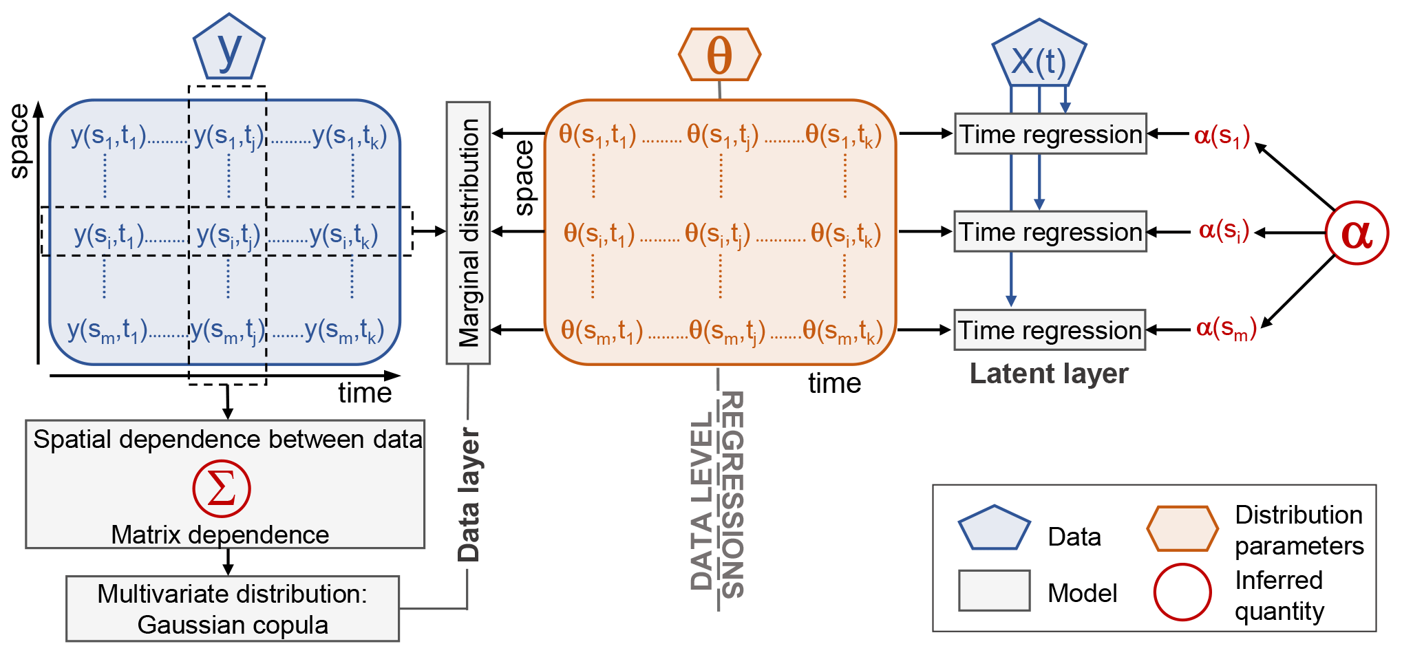
Figure 1 Conceptual sketch of the Bayesian hierarchical model. Blue boxes denote the data, orange boxes the GEV distribution parameters, gray boxes the models, and red circles the inferred quantities. Model boxes correspond to the data layer (Gaussian copula and GEV marginal distributions) and the latent layer (time regressions of GEV parameters). $\mathit{\theta }\left(s_i,t_j\right)=\left[\mathit{\mu }\left(s_i,t_j\right),\log \mathit{\sigma }\left(s_i,t_j\right),\mathit{\xi }\left(s_i,t_j\right)\right]$.

2.2 Marginal distributions

The first two GEV parameters (location and scale) are modeled as linear functions of time-dependent, large-scale climate variables and regional mean variables from the previous season, while the shape parameter is considered to be stationary, as follows:

$$\begin{array}{}\text{(3)}& {\displaystyle }{\mathit{\mu }}_i\left(t\right)={\mathit{\alpha }}_{\mathit{\mu }{\mathrm{0}}_i}+\sum _{j=\mathrm{1}}^n{\mathit{\alpha }}_{\mathit{\mu }{j}_i}{x}_j\left(t\right),i=\mathrm{1},\mathrm{\dots },m\text{(4)}& {\displaystyle }\log \left({\mathit{\sigma }}_i\left(t\right)\right)={\mathit{\alpha }}_{\mathit{\sigma }{\mathrm{0}}_i}+\sum _{j=\mathrm{1}}^n{\mathit{\alpha }}_{\mathit{\sigma }{j}_i}{x}_j\left(t\right),i=\mathrm{1},\mathrm{\dots },m\text{(5)}& {\displaystyle }{\mathit{\xi }}_i={\mathit{\alpha }}_{\mathit{\xi }{\mathrm{0}}_i},i=\mathrm{1},\mathrm{\dots },m,\end{array}$$

where x_j(t) is covariate j at time t, and ${\mathit{\alpha }}_{\mathit{\mu }{j}_i}$, ${\mathit{\alpha }}_{\mathit{\sigma }{j}_i}$, and ${\mathit{\alpha }}_{\mathit{\xi }{\mathrm{0}}_i}$ are the regression coefficients for covariate j and gauge i at time t. log (σ) is used to ensure positive scale parameters. The validity of the nonstationary location and scale parameters can be checked through the significance of their slope coefficients' posterior probability density functions (PDFs; i.e., by checking whether 95 % of the sample values are greater (lower) than 0). Covariates will be discussed in Sect. 3.2. The shape parameter ξ is often modeled as a single value per study area/region because of large estimation uncertainties (Cooley et al., 2007; Renard, 2011; Apputhurai and Stephenson, 2013; Atyeo and Walshaw, 2012), or it is modeled spatially, along with the other GEV parameters, but considers a specific range of potential values (Cooley and Sain, 2010; Bracken et al., 2016). Here, we model the shape parameter for each catchment individually but consider it to be stationary in time.

2.3 Gaussian copula for spatial dependence

Copulas are a flexible tool for modeling multivariate random variables since they can represent dependence independently of the choice of marginal distributions (Genest and Favre, 2007; Bracken et al., 2018; Brunner et al., 2019), which is a particularly appealing feature for extremal processes. This study focuses on Gaussian copulas because of their ease of implementation in a Bayesian and high-dimensional framework.

Let $\mathit{q}\left(t\right)={\left[q_i\left(t\right)\right]}_{i=\mathrm{1}}^m$ be a random vector of extreme streamflow at m gauges and time t. The Gaussian copula builds the joint cumulative distribution function (CDF) of q(t) as follows:

$$\begin{array}{}\text{(6)}& F_{\mathrm{cop}}\left(\mathit{q}\left(t\right)\right)={\mathrm{\Phi }}_{\mathrm{\Sigma }}\left(\mathit{u}\left(t\right)\right),\end{array}$$

where Φ_Σ(⋅) is the joint CDF of an m-dimensional multivariate normal distribution with dependence matrix Σ, $\mathbf{u}\left(t\right)={\left[u_i\left(t\right)\right]}_{i=\mathrm{1}}^m$, $u_i\left(t\right)={\mathrm{\Phi }}^{-\mathrm{1}}\left(F_{it}\left[q_i\left(t\right)\right]\right)$, with Φ being the CDF of the standard normal distribution, and F_it(⋅) is the marginal GEV or empirical CDF for streamflow gauge i at time t.

The copula dependence matrix, Σ, is a symmetric positive definite matrix that captures the strength of dependence between all gauge pairs using the Pearson correlation coefficient. The element c_ij of Σ quantifies the dependence between gauges i and j and its values can vary between −1 and 1, as follows:

$$\begin{array}{}\text{(7)}& \mathbf{\Sigma }=\left[\begin{array}{ccccc}\mathrm{1}& c_{\mathrm{12}}& \mathrm{\cdots }& c_{\mathrm{1}(m-\mathrm{1})}& c_{\mathrm{1}m}\\ c_{\mathrm{21}}& \mathrm{1}& \mathrm{\ddots }& \mathrm{⋮}& c_{\mathrm{2}m}\\ c_{\mathrm{31}}& c_{\mathrm{32}}& \mathrm{\ddots }& \mathrm{⋮}& \mathrm{⋮}\\ \mathrm{⋮}& \mathrm{⋮}& \mathrm{\ddots }& \mathrm{1}& c_{(m-\mathrm{1})m}\\ c_{m\mathrm{1}}& c_{m\mathrm{2}}& \mathrm{\cdots }& c_{m(m-\mathrm{1})}& \mathrm{1}\end{array}\right].\end{array}$$

By definition, the dependency between a streamflow gauge and itself is unity, so the diagonal elements of Σ are a series of ones. Since Σ is symmetric, only $m(m-\mathrm{1})/\mathrm{2}$ values need to be fitted (values in the lower or upper triangle of Σ). The Gaussian copula only assumes a linear correlation after quantile transformation of the marginals with the inverse normal CDF. This does not impose a linear correlation structure on the marginal distributions, meaning that nonlinear dependence between variables can be captured at the data level (Bracken et al., 2018).

There are two main approaches to estimate the unknown parameters of the conditional copula (Hochrainer-Stigler, 2020). The first one is called inference functions for margins (IFMs). In this approach, the marginal distribution parameters are estimated in the first step and the copula parameters in the second step. One major disadvantage of this approach is the loss of estimation efficiency as, in the first step, the dependence between the marginal distributions is not considered. The second approach (hereafter referred to as the pseudo-observations fitting) estimates the copula parameters without assuming specific parametric distribution functions of the marginals, and pseudo-observations are used instead. The framework proposed here considers pseudo-observations fitting to estimate the copula dependence parameters.

2.4 Estimation strategy

The inference of the model parameters is done in a Bayesian framework, which can account for parameter uncertainties. The posterior distributions of the model parameters, $\mathit{\theta }=\left[\mathit{\mu },\log \mathit{\sigma },\mathit{\xi }\right]$ and Σ, given the data (3 d spring maximum (May–June) streamflow at each gauge and covariates) and considering a record length of k days by Bayes' rule, are as follows:

$$\begin{array}{}\text{(8)}& \begin{array}{rl}p& \left(\mathit{\theta },\mathbf{\Sigma }|\mathit{q},\mathit{x},\mathit{u}\right)\\ & \propto \left[\prod _{t=\mathrm{1}}^k\left(\prod _{i=\mathrm{1}}^m{p}_q\left(\left.q_i\left(t\right)\right|{\mathit{\theta }}_i,\mathit{x}\left(t\right)\right)\right)p_u\left(\left.\mathit{u}\left(t\right)\right|\mathbf{\Sigma }\right)\right]\\ & p_{\mathit{\theta }}\left(\mathit{\theta }\right)p_{\mathrm{\Sigma }}\left(\mathbf{\Sigma }\right),\end{array}\end{array}$$

where p_q(q_i(t)|θ_i,x(t)) represents the PDF of the GEV for location i and time t, $p_u\left(\left.\mathit{u}\left(t\right)\right|\mathbf{\Sigma }\right)=\mathrm{MVN}\left(\left.\mathit{u}\left(t\right)\right|\mathbf{0},\mathbf{\Sigma }\right)$ is the Gaussian copula PDF for time t, $u\left(t\right)={\left[u_i\left(t\right)\right]}_{i=\mathrm{1}}^m$, $u_i\left(t\right)={\mathrm{\Phi }}^{-\mathrm{1}}\left(F_{it}\left[q_i\left(t\right)\right]\right)$, Φ is the CDF of the standard normal distribution, F_it(⋅) is the empirical CDF (pseudo-observations) for location i at time t, and p_Σ( Σ) and p_θ(θ) represent the priors of the GEV regression coefficients and Gaussian copula dependence matrix, respectively. p_θ(θ) is defined as follows:

$$\begin{array}{}\text{(9)}& {\displaystyle }{p}_{\mathit{\theta }}\left(\mathit{\theta }\right)=p_{\mathit{\mu }}\left(\mathit{\mu }\right)p_{\mathit{\sigma }}\left(\log \mathit{\sigma }\right)p_{\mathit{\xi }}\left(\mathit{\xi }\right)\text{(10)}& {\displaystyle }{p}_{\mathit{\mu }}\left(\mathit{\mu }\right)=\prod _{j=\mathrm{0}}^n\mathrm{MVN}\left(\left.{\mathit{\alpha }}_{{\mathit{\mu }}_j}\right|\mathbf{0},{\mathbf{\Sigma }}_{{\mathit{\alpha }}_{{\mathit{\mu }}_j}}\right)p_{{\mathrm{\Sigma }}_{{\mathit{\alpha }}_{{\mathit{\mu }}_j}}}\left({\mathbf{\Sigma }}_{{\mathit{\alpha }}_{{\mathit{\mu }}_j}}\right)\text{(11)}& {\displaystyle }{p}_{\mathit{\sigma }}\left(\log \mathit{\sigma }\right)=\prod _{j=\mathrm{0}}^n\mathrm{MVN}\left(\left.{\mathit{\alpha }}_{{\mathit{\sigma }}_j}\right|\mathbf{0},{\mathbf{\Sigma }}_{{\mathit{\alpha }}_{{\mathit{\sigma }}_j}}\right)p_{{\mathrm{\Sigma }}_{{\mathit{\alpha }}_{{\mathit{\sigma }}_j}}}\left({\mathbf{\Sigma }}_{{\mathit{\alpha }}_{{\mathit{\sigma }}_j}}\right)\text{(12)}& {\displaystyle }{p}_{\mathit{\xi }}\left(\mathit{\xi }\right)=\mathrm{MVN}\left(\left.{\mathit{\alpha }}_{{\mathit{\xi }}_{\mathrm{0}}}\right|\mathbf{0},{\mathbf{\Sigma }}_{{\mathit{\alpha }}_{{\mathit{\xi }}_{\mathrm{0}}}}\right)p_{{\mathrm{\Sigma }}_{{\mathit{\alpha }}_{{\mathit{\xi }}_{\mathrm{0}}}}}\left({\mathbf{\Sigma }}_{{\mathit{\alpha }}_{{\mathit{\xi }}_{\mathrm{0}}}}\right),\end{array}$$

where MVN$\left(\left.{\mathit{\alpha }}_{{\mathit{\mu }}_j}\right|\mathbf{0},{\mathbf{\Sigma }}_{{\mathit{\alpha }}_{{\mathit{\mu }}_j}}\right)$, MVN$\left(\left.{\mathit{\alpha }}_{{\mathit{\sigma }}_j}\right|\mathbf{0},{\mathbf{\Sigma }}_{{\mathit{\alpha }}_{{\mathit{\sigma }}_j}}\right)$, and MVN$\left(\left.{\mathit{\alpha }}_{{\mathit{\xi }}_{\mathrm{0}}}\right|\mathbf{0},{\mathbf{\Sigma }}_{{\mathit{\alpha }}_{{\mathit{\xi }}_{\mathrm{0}}}}\right)$ represent probability densities of multivariate normal distributions with mean 0 and covariance matrices ${\mathbf{\Sigma }}_{{\mathit{\alpha }}_{{\mathit{\mu }}_j}}$, ${\mathbf{\Sigma }}_{{\mathit{\alpha }}_{{\mathit{\sigma }}_j}}$, and ${\mathbf{\Sigma }}_{{\mathit{\alpha }}_{{\mathit{\xi }}_{\mathrm{0}}}}$ correspond to the priors of the GEV regression coefficients ${\mathit{\alpha }}_{{\mathit{\mu }}_j}$, ${\mathit{\alpha }}_{{\mathit{\sigma }}_j}$, and ${\mathit{\alpha }}_{{\mathit{\xi }}_{\mathrm{0}}}$, respectively. $p_{{\mathrm{\Sigma }}_{{\mathit{\alpha }}_{{\mathit{\mu }}_j}}}\left({\mathbf{\Sigma }}_{{\mathit{\alpha }}_{{\mathit{\mu }}_j}}\right)$, $p_{{\mathrm{\Sigma }}_{{\mathit{\alpha }}_{{\mathit{\sigma }}_j}}}\left({\mathbf{\Sigma }}_{{\mathit{\alpha }}_{{\mathit{\sigma }}_j}}\right)$, and $p_{{\mathrm{\Sigma }}_{{\mathit{\alpha }}_{{\mathit{\xi }}_{\mathrm{0}}}}}\left({\mathbf{\Sigma }}_{{\mathit{\alpha }}_{{\mathit{\xi }}_{\mathrm{0}}}}\right)$ are the priors of ${\mathbf{\Sigma }}_{{\mathit{\alpha }}_{{\mathit{\mu }}_j}}$, ${\mathbf{\Sigma }}_{{\mathit{\alpha }}_{{\mathit{\sigma }}_j}}$, and ${\mathbf{\Sigma }}_{{\mathit{\alpha }}_{{\mathit{\xi }}_{\mathrm{0}}}}$, which, based on Gelman and Hill (2006), are assumed to follow an inverse Wishart distribution to ensure a positive definite covariance matrix as follows:

$$\begin{array}{}\text{(13)}& {\displaystyle }{\mathbf{\Sigma }}_{{\mathit{\alpha }}_{{\mathit{\mu }}_j}}\sim \mathrm{Inv}\mathrm{wishart}\left(\mathit{\nu },A_j\mathit{I}\right)\text{(14)}& {\displaystyle }{\mathbf{\Sigma }}_{{\mathit{\alpha }}_{{\mathit{\sigma }}_j}}\sim \mathrm{Inv}\mathrm{wishart}\left(\mathit{\nu },B_j\mathit{I}\right)\text{(15)}& {\displaystyle }{\mathbf{\Sigma }}_{{\mathit{\alpha }}_{{\mathit{\xi }}_{\mathrm{0}}}}\sim \mathrm{Inv}\mathrm{wishart}\left(\mathit{\nu },C_{\mathrm{0}}\mathit{I}\right).\end{array}$$

ν corresponds to the degrees of freedom (m+1), I is an $(m+\mathrm{2})\times (m+\mathrm{2})$ identity matrix, and A_j, B_J, and C₀ are scalars properly set for ${\mathbf{\Sigma }}_{{\mathit{\alpha }}_{{\mathit{\mu }}_j}}$, ${\mathbf{\Sigma }}_{{\mathit{\alpha }}_{{\mathit{\sigma }}_j}}$, and ${\mathbf{\Sigma }}_{{\mathit{\alpha }}_{{\mathit{\xi }}_{\mathrm{0}}}}$, respectively. The regression coefficients are modeled jointly to capture their spatial correlations. Finally, p_Σ(Σ) represents the prior of the Gaussian copula dependence matrix and is also assumed to follow an inverse Wishart distribution to ensure a positive definite covariance matrix as follows:

$$\begin{array}{}\text{(16)}& \mathbf{\Sigma }\sim \mathrm{Inv}\mathrm{wishart}\left(\mathit{\nu },{\mathit{C}}_{\mathrm{u}}\right),\end{array}$$

where C_u corresponds to the covariance matrix of the uniform quantiles obtained from the pseudo-observations.

2.5 Estimation of ensembles of seasonal streamflow projections

The predictive posterior distribution of the spring maximum streamflow (ensembles) for the m streamflow gauges can be estimated using the posterior distributions (M samples) of GEV regression coefficients, ${\mathit{\alpha }}_{{\mathit{\mu }}_j}$, ${\mathit{\alpha }}_{{\mathit{\sigma }}_j}$, and ${\mathit{\alpha }}_{{\mathit{\xi }}_{\mathrm{0}}}$, and the Gaussian copula dependence matrix, Σ, which have been estimated using the estimation strategies presented in the previous section. To estimate the spring maximum streamflow ensemble members, for each posterior sample of all model parameters (${\mathit{\alpha }}_{{\mathit{\mu }}_j}$, ${\mathit{\alpha }}_{{\mathit{\sigma }}_j}$, ${\mathit{\alpha }}_{{\mathit{\xi }}_{\mathrm{0}}}$, and Σ), the procedure is as follows:

1. If the posterior PDFs of the slope coefficients of the GEV parameters were found to be significant, compute the GEV parameters (μ_i(t), log (σ_i(t))) for each year and gauge using ${\mathit{\alpha }}_{{\mathit{\mu }}_i}$ and ${\mathit{\alpha }}_{{\mathit{\sigma }}_i}$, and covariates, x(t), using Eqs. (3)–(4).

2. Then, simulate the marginal cumulative distributions, F_it, for the m streamflow gauges from a Gaussian copula with a dependence matrix, Σ.

3. Thereafter, compute the spring maximum streamflow for each streamflow gauge i at time t, using the following expression:

   $$\begin{array}{}\text{(17)}& \begin{array}{rl}{q}_i\left(t\right)& ={\mathit{\mu }}_i\left(t\right)+{\displaystyle \frac{{\mathit{\sigma }}_i\left(t\right)}{{\mathit{\xi }}_i}}\left[{\left(-\log \left(F_{it}\right)\right)}^{-{\mathit{\xi }}_i}-\mathrm{1}\right],\\ & i=\mathrm{1},\mathrm{\dots },m,\end{array}\end{array}$$

   where σ_i(t)=exp (log (σ_i(t)).

4. As a final step, repeat steps 2–3 for each gauge and year of the record.

This procedure has to be repeated M times.

3 Application of framework to the Upper Colorado River basin

We demonstrate the utility of the framework proposed in the previous section by applying it to project 3 d spring maximum (May–June) streamflow at seven gauges in the Upper Colorado River basin (UCRB) with 0- to 2-month lead time (Fig. 2). The UCRB is located in west-central Colorado, USA, and has an area of approximately 25 700 km². Its headwaters originate at the Continental Divide in the Rocky Mountain National Park. Further downstream, UCRB flows in a westerly direction through forested mountains and irrigated valleys before it leaves Colorado in Mesa County downstream of the city of Grand Junction (Colorado's Decision Support Systems, 2007). The basin has a snowmelt-dominated flow regime, i.e., most of the precipitation is accumulated during winter in the form of snow. Over 85 % of the basin's streamflow and flood peaks occur in spring due to snowmelt. Therefore, using snow information of the basin might provide skillful projections of spring maximum streamflow several months in advance.

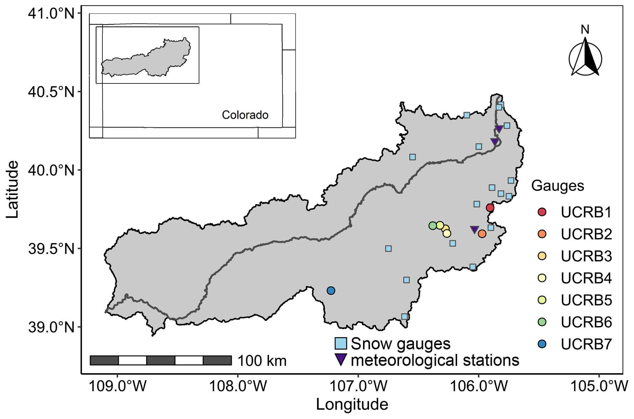
Figure 2 Streamflow gauges in the Upper Colorado River basin (UCRB) considered in this study. Light blue squares correspond to the snow gauges (18) and purple triangles to the meteorological stations (3) considered in this study.

3.1 Streamflow data

Daily spring, May through June, streamflow data were obtained from the U.S. Geological Survey (USGS) using the R package dataRetrieval (De Cicco et al., 2018). We selected streamflow gauges located inside the UCRB with no more than 10 % or 3 consecutive years of missing data from 1965 to 2018. This procedure resulted in the selection of seven streamflow gauges (Fig. 2 and Table 1). The seven gauges have drainage areas between 14.5 and 432.5 km², elevations between 2105 and 3179 m. a.s.l. (above sea level), and mean streamflow and mean seasonal (May–June) streamflow range from 1 to 28.3 m³ s⁻¹ and from 0.3 to 8.3 m³ s⁻¹, respectively. The seven catchments are not nested; instead, they are individual subcatchments of the larger UCRB. We computed 3 d spring maximum streamflow for each year at each streamflow gauge. For a gauge with missing annual values, these values were substituted with the gauge's median value.

Figure 3 shows the spatial dependence of 3 d spring maximum streamflow for the seven gauges, which was assessed using Kendall's rank correlation for each pair of stations. The dependence of 3 d spring maximum streamflows between gauges is generally positive, as indicated by Kendall's rank correlation values higher than 0.4 (significant at 95 % confidence level) for all station pairs. These significant spatial correlations require the inclusion of a copula in the BHM to capture the spatial dependence of the data.

Table 1 Basic data corresponding to the streamflow gauges in the Upper Colorado River basin (UCRB) considered in this study.

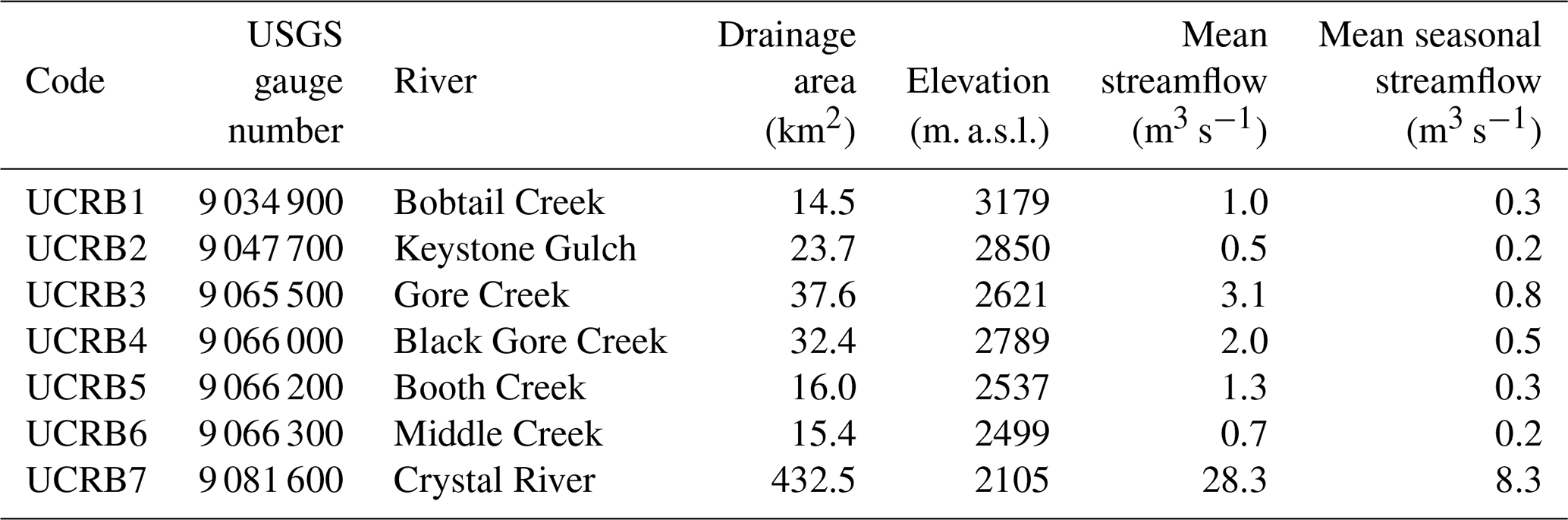
Figure 3 Pairs plot (lower triangular matrix) and Kendall's rank correlation coefficients (upper triangular matrix) of spring 3 d maximum streamflow between the seven stations in the UCRB. Kendall's rank correlation is significant (p values < 0.1), and positive association patterns are visible for all pairs.

3.2 Covariates

It has been shown in previous studies that the snow water equivalent (SWE) accumulated until the beginning of spring is the most skillful predictor of spring–summer seasonal streamflow across mountainous regions, such as the western USA (Koster et al., 2010; Pagano, 2010; Wood et al., 2016; Livneh and Badger, 2020). Other potentially useful predictors might include sea surface temperature anomalies or atmospheric teleconnection patterns. For the Colorado River, strong links between annual flow and large-scale climate drivers have been documented, e.g., with the Atlantic Multidecadal Oscillation (AMO; McCabe and Dettinger, 1999; Enfield et al., 2001; Hidalgo, 2004; Tootle et al., 2005; McCabe et al., 2007; Timilsena et al., 2009; Nowak et al., 2012), the Pacific Decadal Oscillation (PDO; Hidalgo, 2004; Tootle et al., 2005; Timilsena et al., 2009), and the El Niño–Southern Oscillation (ENSO; Redmond and Koch, 1991; Kahya and Dracup, 1994; Rajagopalan et al., 2000; Thomson et al., 2003; Timilsena et al., 2009). However, the relationship of these indices with annual or seasonal extremes has not been explored in-depth, and earlier studies shown modest relationships, e.g., between southwestern USA seasonal or annual maximum streamflow and ENSO and PDO (Sankarasubramanian and Lall, 2003; Werner et al., 2004).

We test the usefulness of both snow-related and climatic drivers within the BHM framework by using SWE and different climatic indices as potential covariates of the marginal GEV distributions. Specifically, we tested the following covariates for modeling the temporal nonstationarity of the GEV parameters (see Eqs. 3–4) for the period 1965–2018, including the average ENSO, PDO, and AMO climate indices, the spatial average of accumulated snow water equivalent (SASWE) from November to February, March, or April, depending on the lead time (0-, 1-, or 2-month lead time), and the spatial average April mean temperature (SAAMT). As indicated earlier, we focus on projecting 3 d extreme spring streamflow at lead times of 0-, 1- and 2-months, corresponding to forecast issuance on 1 May, 1 April, and 1 March, respectively (Fig. 4). The covariates use all information prior to forecast issuance. We did not consider spatial average precipitation as covariate since it can not be well predicted ahead of more than 2 weeks (Werner and Yeager, 2013).

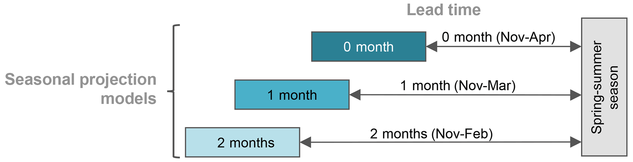
Figure 4 Schemes of nonstationary models considered for three different lead times. The dark turquoise box denotes the model for a 0-month lead time (projections are released on 1 May), the turquoise box the model for a 1-month lead time (projections are released on 1 April), and the light turquoise box the model for a 2-month lead time (projections are released on 1 March). The same color scheme will be considered for the Sect. 4.

The potential covariates – monthly ENSO, PDO, and AMO climate indices, monthly accumulated SWE from November to April, and daily mean temperature for April – were computed using the following data sources:

1. ENSO, PDO, and AMO climate indices are from the National Oceanic and Atmospheric Administration (NOAA; https://psl.noaa.gov/data/climateindices/list/, last access: 16 June 2021).

2. SWE is from the Natural Resources Conservation Service (NRCS) Snow Course Data (https://wcc.sc.egov.usda.gov/reportGenerator/, last access: 16 June 2021).

3. April's daily mean temperature is from the Global Historical Climatology Network (GHCN; Menne et al., 2012).

For SWE and daily mean temperature, we only considered snow gauges (18) and meteorological stations (3) located inside the UCRB with full records for the period of interest (1965-2018; see Fig. 2). We then computed the SASWE and SAAMT covariates as the mean across all snow gauges and meteorological stations for each year, respectively. We considered the same SWE (SASWE) and April mean temperature (SAAMT) covariates for all the gauges because these regional variables do not rely on one single station, which may not necessarily stay in operation, and they can capture the spring maximum streamflow signal for all the station gauges. For example, suppose that, in the future, a particular snow gauge is out of operation. In that case, one can keep using the average of the operative snow gauges and still derive the covariate. Figure 5 displays the time series of normalized spring maximum streamflow with the SASWE (SAAMT) covariate and the best local SWE (AMT) covariate, respectively, for the station UCRB1. The two regional covariates can capture the interannual variability in the spring maximum streamflow without an important reduction in the correlation compared to local covariates. The suitability of the regional covariates is also verified for the other catchments and lead times.

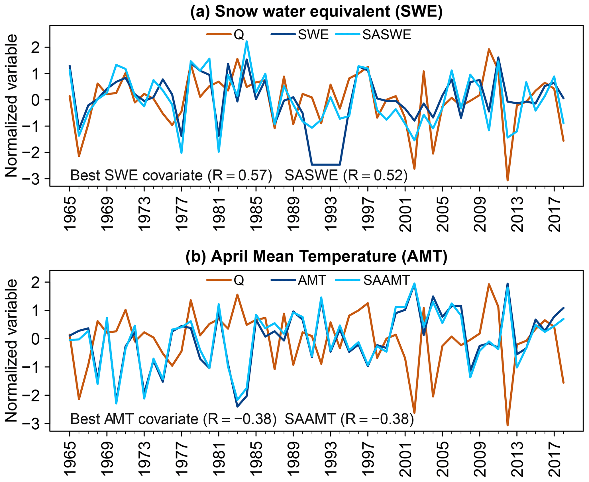
Figure 5 Time series of normalized 3 d spring maximum streamflow, best covariate, and the spatial average covariate of (a) accumulated snow water equivalent until 30 April (SWE) and (b) mean April temperature (AMT) for UCRB1. At the bottom of each panel, the correlation of 3 d maximum streamflow with the regional and the best local (i.e., highest correlation) covariate are displayed.

We assessed the strength of the relationship between the covariates and spring maximum streamflow by computing the Spearman's rank correlation coefficient, which is shown in Fig. 6 for a 0-month lead time (covariates were calculated from November to April). SASWE (Fig. 6a) exhibits a significant and strong positive correlation with a spring maximum streamflow at all the gauges, which was expected and also supports the choice of SASWE as a covariate for all the station gauges. At the same time, SAAMT (Fig. 6b) shows a significant negative correlation with the spring maximum streamflow. This finding was also expected, since a higher mean April temperature would lead to early melt and, therefore, less snow availability for melt later in spring. The ENSO, PDO, and AMO climate indices (Fig. 6c–e) show a weaker correlation with the spring maximum streamflow than SASWE and SAAMT at almost all the gauges. Similar correlations were found for other lead times (Figs. S1 and S2 in the Supplement). For each lead time, we obtained the best nonstationary GEV model as the combination of predictors that resulted in a minimum deviance information criterion (DIC; Spiegelhalter et al., 2002). The DIC corresponds to a hierarchical modeling generalization of the Akaike information criterion (AIC; Akaike, 2011) and facilitates the Bayesian model selection. The DIC is computed for a suite of candidate models with various combinations of covariates, and the model with the minimum DIC is selected for predicting spring maximum streamflow in the UCRB.

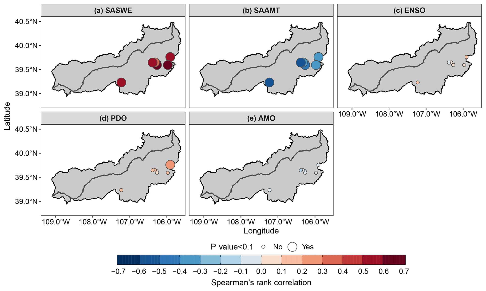
Figure 6 Spearman's rank correlation coefficient between 3 d spring maximum streamflow and potential covariates for a 0-month lead time. (a) The spatial average of November–April snow water equivalent (SASWE) over the UCRB. (b) The spatial average of April mean temperature (SAAMT) over the UCRB. (c) Mean November–April ENSO. (d) Mean November–April PDO. (e) Mean November–April AMO. Big circles indicate that Spearman's rank correlation is significant (p value < 0.1).

3.3 Suitability of the GEV distribution and Gaussian copula

We checked the suitability of the GEV distribution as a marginal distribution and of the Gaussian copula as a spatial dependence model using their maximum likelihood estimates for 3 d spring maximum streamflow.

To check the validity of the GEV distribution as a marginal distribution, we fitted a stationary GEV distribution at each gauge using maximum likelihood. Then, we ran two goodness-of-fit tests, i.e., the Cramér–von Mises and Anderson–Darling tests (D'Agostino and Stephens, 1986). The p values for the two tests were higher than 0.3 for most of the gauges, except for UCRB1 (0.11), which implies that, at the 95 % confidence level, there is insufficient evidence to reject the null hypothesis that the data come from a GEV distribution. Q–Q plots of the stationary GEV distribution fitted to 3 d spring maximum streamflow for the seven streamflow gauges of UCRB can be found in Fig. S3.

For testing the suitability of the Gaussian copula, we ran three multivariate normality tests using marginal transformations based on pseudo-observations from the tests of Royston (1982), Mardia (1970), and Henze and Zirkler (1990). The p values obtained for the three tests were 0.27, 0.45, and 0.6, respectively, which did not reject the null hypothesis that the transformed data follow a multivariate normal distribution. As an illustration of the goodness fit of the Gaussian copula, Fig. 7 shows the pairwise dependence structure between gauges UCRB2 and UCRB4 for different copula families (for more details about the other types of copulas, the reader is referred to Hochrainer-Stigler, 2020, or Genest and Favre, 2007). The black points in each panel (Fig. 7b–g) correspond to the observed CDF values. The simulated contour lines represent simulated contour lines for different dependence structures, including independence (no copula; Fig. 7b), Gaussian (Fig. 7c), Student t (Fig. 7d), Joe (Fig. 7e), Gumbel (Fig. 7f), and Vine copulas (Fig. 7g). Only Gaussian, Student t, and Vine copulas can capture the dependence structure of the data. This visual inspection confirms that the Gaussian copula is suitable for replicating the dependence structure of the observed data.

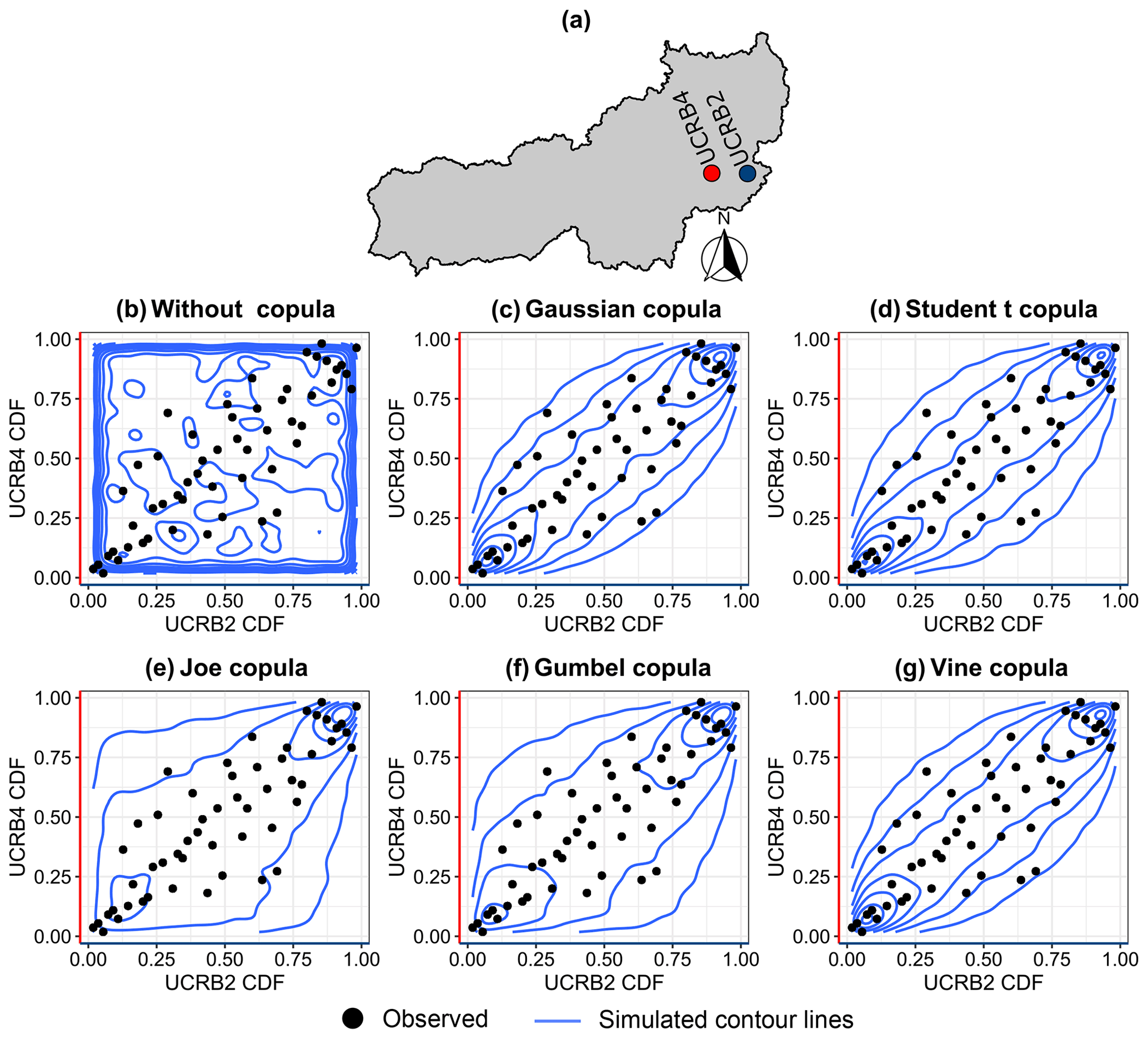
Figure 7 Pairwise dependence structure between UCRB2 and UCRB4 (a) streamflow simulated (b) without a copula and with a (c) Gaussian copula, (d) Student t copula, (e) Joe copula, (f) Gumbel copula, and (g) Vine copula. Observations and simulated contour lines are shown as black points and blue lines, respectively.

3.4 Model structure for the UCRB

The specific structure of the BHM for the UCRB incorporates the covariates described in Sect. 3.2. We modeled the location parameter of the GEV at each gauge in a nonstationary way, but the scale parameter of the GEV is kept stationary for all gauges. An initial run of the BHM with a nonstationary scale parameter showed that the regression coefficients (${\mathit{\alpha }}_{{\mathit{\sigma }}_j}=\mathrm{0}$ for j>0 in Eq. 4) were not significant (posterior PDFs contain zero in the 95 % confidence interval). The priors of the covariance matrix of ${\mathit{\alpha }}_{{\mathit{\mu }}_j}$, ${\mathit{\alpha }}_{{\mathit{\sigma }}_{\mathrm{0}}}$, and ${\mathit{\alpha }}_{{\mathit{\xi }}_{\mathrm{0}}}$ used are as follows:

$$\begin{array}{}\text{(18)}& {\displaystyle }{\mathbf{\Sigma }}_{{\mathit{\alpha }}_{{\mathit{\mu }}_{\mathrm{0}}}}\sim \mathrm{Inv}\mathrm{wishart}\left(\mathrm{8},A_{\mathrm{0}}\mathit{I}\right)\text{(19)}& {\displaystyle }{\mathbf{\Sigma }}_{{\mathit{\alpha }}_{{\mathit{\mu }}_j}}\sim \mathrm{Inv}\mathrm{wishart}\left(\mathrm{8},A_j\mathit{I}\right),j\ge \mathrm{1}\text{(20)}& {\displaystyle }{\mathbf{\Sigma }}_{{\mathit{\alpha }}_{{\mathit{\sigma }}_{\mathrm{0}}}}\sim \mathrm{Inv}\mathrm{wishart}\left(\mathrm{8},B_{\mathrm{0}}\mathit{I}\right)\text{(21)}& {\displaystyle }{\mathbf{\Sigma }}_{{\mathit{\alpha }}_{{\mathit{\xi }}_{\mathrm{0}}}}\sim \mathrm{Inv}\mathrm{wishart}\left(\mathrm{8},C_{\mathrm{0}}\mathit{I}\right).\end{array}$$

We considered noninformative priors for the covariance matrix of the GEV regression coefficients by setting A₀=100, A_j=10, B₀=1, and C₀=1. Since we fitted different types of BHMs, ${\mathbf{\Sigma }}_{{\mathit{\alpha }}_j}$ is only considered for nonstationary models. For the dependence matrix of the Gaussian copula, we used an informative prior as follows:

$$\begin{array}{}\text{(22)}& \mathbf{\Sigma }\sim \mathrm{Inv}\mathrm{wishart}\left(\mathrm{8},{\mathit{C}}_{\mathrm{u}}\right),\end{array}$$

where C_u corresponds to the covariance matrix of the uniform quantiles obtained from the pseudo-observations of spring maximum streamflow.

3.5 Implementation and model fitting

The model was implemented in R (R Core, 2017), using the program JAGS (Just Another Gibbs Sampler; Plummer, 2003) and the R package rjags (Plummer, 2019), which provides an interface from R to the JAGS library for Bayesian data analysis. Posterior distributions of the GEV regression coefficients and Gaussian copula matrix were estimated using Gibbs sampling (Gelman and Hill, 2006; Robert and Casella, 2011), based on the priors assigned in the previous section. The predictive posterior distributions of spring maximum streamflow (ensembles) for all years were estimated according to Sect. 2.5. We ran three parallel chains with different initial values, and each simulation was performed for 2 000 000 iterations, with a burn-in size value of 1 000 000 to ensure convergence. To reduce the sample dependence (autocorrelation), the thinning factor was set to 500, which yields 6000 samples (2000 samples from each chain). The scale reduction factor $\widehat{R}$ (Gelman and Rubin, 1992) was used to check for model convergence, i.e., $\widehat{R}$ values less than the critical value of 1.1 suggest the adequate convergence of the model. In all of our runs, the $\widehat{R}$ values were less than 1.1 in 6000 samples, indicating convergence. Consequently, the posterior distributions of the GEV regression coefficients, the Gaussian copula matrix, and the predictive posterior distributions of spring maximum streamflow consisted of 6000 ensembles.

3.6 Model cross-validation and verification metrics

To test the out-of-sample predictability of the model, we performed a leave‐1‐year‐out cross-validation by dropping 1 year from the record (1965–2018) and fitting the BHM using the remaining years, which are also known as the calibration years. The fitted model is applied to provide estimates for the 1 validation year. This cross‐validation procedure was repeated 54 times.

As the goal of this study is to provide seasonal streamflow extremes projections for risk-based flood adaptation, we also implemented this leave‐1‐year‐out cross-validation just for high-flow years in which all the station gauges exceeded their 60th percentile.

We computed the energy skill score (ESS) as our verification metric, since we are interested in capturing the spatiotemporal dependence of the data. The energy score (ES) assesses the probabilistic forecasts of a multivariate quantity, as follows (Gneiting and Raftery, 2007; Gneiting et al., 2008):

$$\begin{array}{}\text{(23)}& \mathrm{ES}={\displaystyle \frac{\mathrm{1}}{M}}\sum _{j=\mathrm{1}}^M\left|\right|{\mathit{q}}_j-{\mathit{q}}_{\mathrm{o}}\left|\right|-{\displaystyle \frac{\mathrm{1}}{\mathrm{2}{M}^{\mathrm{2}}}}\sum _{i=\mathrm{1}}^M\sum _{j=\mathrm{1}}^M\left|\right|{\mathit{q}}_i-{\mathit{q}}_j\left|\right|,\end{array}$$

where M=3000 is the size of the ensemble forecast, q_j is the 7×1 vector of the jth ensemble forecast at year t, q_o is the 7×1 vector of observed streamflow at year t, and $\left|\right|\cdot \left|\right|$ denotes the Euclidean norm. This performance metric is a direct generalization of the continuous ranked probability score (CRPS; Gneiting and Raftery, 2007; Gneiting et al., 2008), which reduces the energy score in dimension d=1. Based on ES, the energy skill score (ESS) is defined as follows:

$$\begin{array}{}\text{(24)}& \mathrm{ESS}=\mathrm{1}-{\displaystyle \frac{\stackrel{\mathrm{‾}}{{\mathrm{ES}}_{\mathrm{projection}}}}{\stackrel{\mathrm{‾}}{{\mathrm{ES}}_{\mathrm{reference}}}}},\end{array}$$

where $\stackrel{\mathrm{‾}}{{\mathrm{ES}}_{\mathrm{projection}}}$ is the mean ES of the projection model analyzed, and $\stackrel{\mathrm{‾}}{{\mathrm{ES}}_{\mathrm{reference}}}$ is the mean ES of the reference projection. The ESS ranges from −∞ to 1. ESS < 0 indicate that the reference projection has higher skill than the projection model, ESS = 0 implies equal skill, and ESS > 0 means that the projection model has a higher skill, with ESS = 1 representing a perfect score. For this study, we considered the climatology (sampling from the observations) as the reference projection and benchmark. ESS was computed for both the calibration and validation models.

4 Results

4.1 Selection of the best model for each lead time

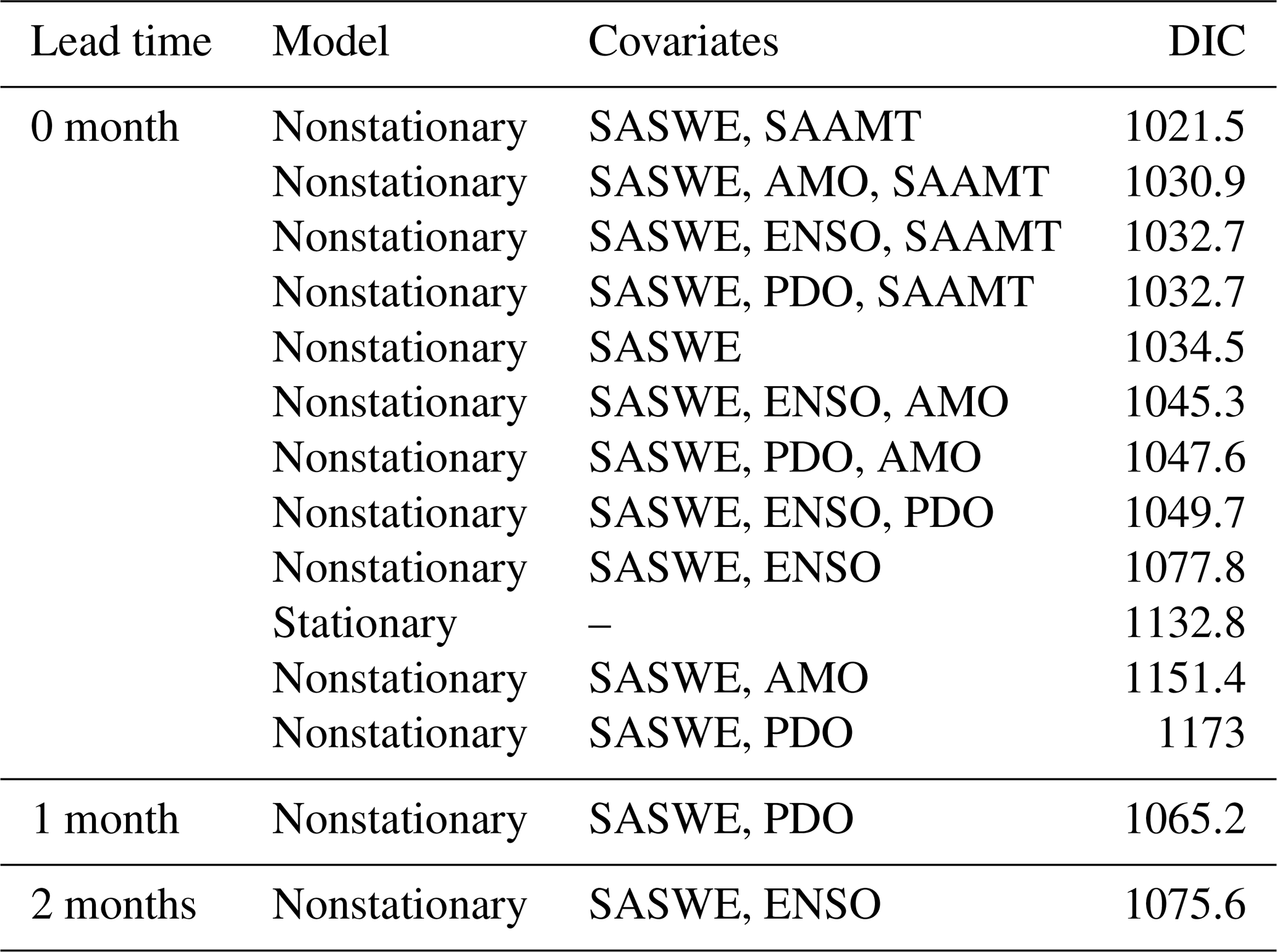
For each lead time, different candidate BHMs were calibrated for the period 1965–2018, and the best BHM was selected based on the lowest DIC value. Table 2 shows the DIC values for different candidate BHMs for a 0-month lead time and the best model for the other two lead times (last two rows). In the case of a 0-month lead time, the best model corresponds to the first row of Table 2. For a 0-month lead time, the predictive skill resides in SWE and air temperature, as this hydroclimatic information relates well to the streamflow extremes in May–June (see Fig. 6). However, for longer lead times of 1 and 2 months, the large-scale climate indices add predictive value. All the models fitted consider a Gaussian copula to model spatial dependence. Detailed tables with different models fitted for 1- and 2-month lead times can be found in Tables S1 and S2.

Table 2 DIC values for different candidate BHMs for a 0-month lead time and the best model for the other two lead times. For each model, the same covariates for the location parameter are considered at all gauges. Candidate BHMs are sorted from the lowest to the highest DIC value for a 0-month lead time. Scale and shape parameters are considered stationary. All candidate BHMs consider a Gaussian copula to model spatial dependence.

4.2 Ability of the BHM to capture spatiotemporal dependence

To assess the ability of the BHM in capturing the spatiotemporal dependence through nonstationary covariates and a Gaussian copula, we compared the best model for the 0-month lead time selected in the previous section (i.e., SASWE and SAAMT as covariates with a Gaussian copula) against three models that do not consider a Gaussian copula (i.e., stationary, nonstationary with SASWE as covariate, and nonstationary with SASWE and SAAMT as covariates).

Figure 8 shows the energy skill score (ESS) distribution from the calibration (1965–2018) for the four BHMs for a 0-month lead time. Higher values of the ESS indicate better performance. The stationary model (light gray box) performs poorly in capturing the spatiotemporal dependence compared to the benchmark (i.e., values below 0). This model also shows a lower variability in the skill score than the other Bayesian hierarchical models, which is expected because the stationary model produces the same projection for each year. When a nonstationary model with SASWE as a covariate is considered (gray box), then the skill is substantially improved compared to the benchmark and the stationary model (i.e., most of the values above 0). This improvement is consistent with Fig. 6 and previous studies stating that SWE until the beginning of the spring season is the most skillful predictor of spring–summer seasonal streamflow in mountainous regions (Koster et al., 2010; Livneh and Badger, 2020). When SAAMT is added as a covariate (dark gray box), then there is a significant improvement in ESS compared to the model with only SASWE. The best model with copula (dark turquoise box) substantially increases model skill. Model skill increases were tested with a 95 % confidence interval, using a nonparametric test for the median (Gibbons and Chakraborti, 1992).

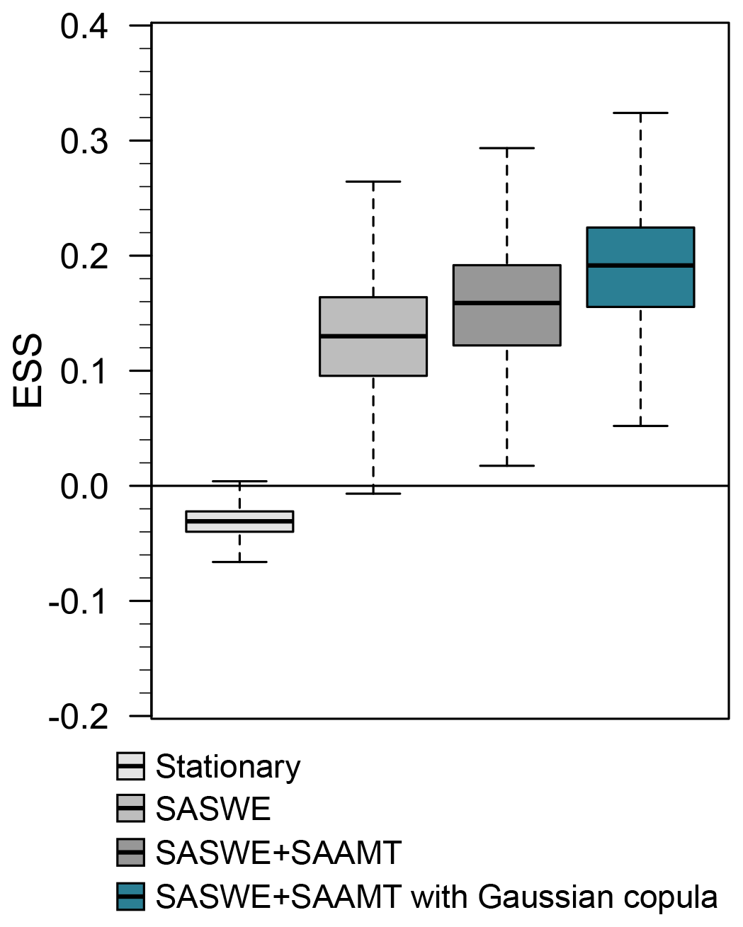
Figure 8 Energy skill score (ESS) distribution for four different BHM versions for a 0-month lead time for the calibration period (1965–2018). Higher values of the ESS indicate better model performance. The whiskers show the 95 % credible intervals, boxes show the interquartile range, and horizontal lines inside the boxes show the median. Outliers are not displayed. The light gray box denotes a stationary model, the gray box a nonstationary model with SASWE as a covariate, the dark gray box a nonstationary model with SASWE and SAAMT as covariates, and the dark turquoise model adds a Gaussian copula to model spatial dependence.

To further highlight the ability of the Gaussian copula to capture the spatiotemporal dependence, we computed the spatial joint threshold non-exceedance probabilities for the seven stations and compared them to non-exceedance probabilities derived from three models without the copula, i.e., spatially independent models for each streamflow gauge. In Fig. 9, we display the distribution of the probability that all streamflow gauges do not exceed their kth percentile for the observations and the four models shown in Fig. 8 for a 0-month lead time and the calibration period. The model with nonstationary covariates and a Gaussian copula (dark turquoise box plots) can almost reproduce the shape of the observed distribution in terms of the interquartile range (boxes), which is an indication that this model can capture the spatiotemporal dependence of the data well. Figure 9 also shows that, even without considering a copula, a nonstationary model with skillful covariates can partially capture the spatiotemporal dependence (see the difference in the distribution shape for the stationary and nonstationary models without copula in Fig. 9). The ability of the nonstationary model to partially capture the spatiotemporal dependence suggests that, with the increasing skill of the covariates, the added value of the copula becomes smaller. Similar performance was observed for the nonstationary model, with SASWE as a covariate plus a Gaussian copula, and for a nonstationary model, with a less skillful covariate (ENSO) plus a Gaussian copula (not shown here).

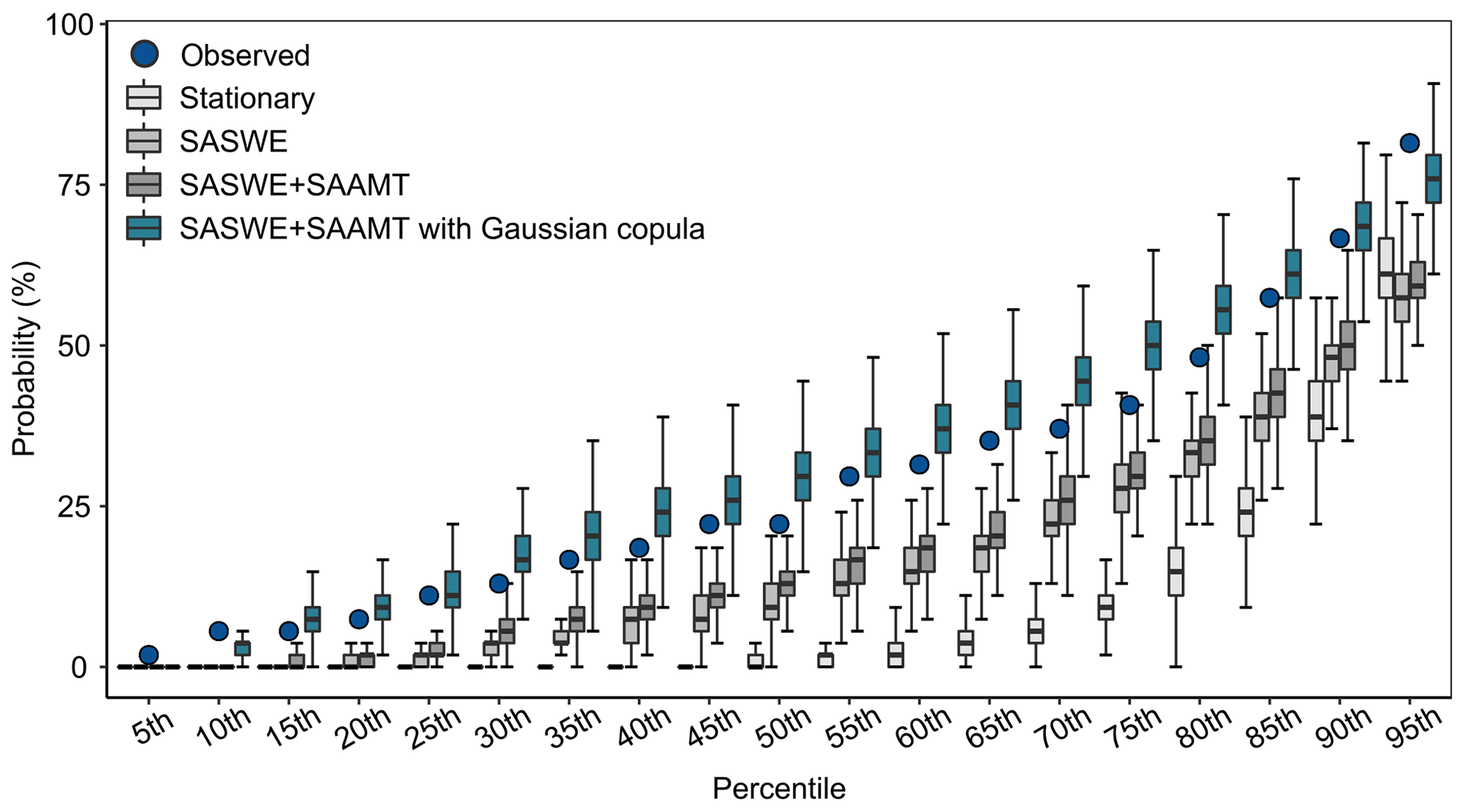
Figure 9 Distribution of the probability that all gauges do not exceed their kth percentile for four different versions of the BHM for a 0-month lead time for the calibration period (1965–2018). The whiskers show the 95 % credible intervals, boxes show the interquartile range, and horizontal lines inside the boxes show the median. Outliers are not displayed. The observations are shown as blue circles, and the same color scheme as in Fig. 8 is considered for the four versions of the BHM.

In order to assess the spatial performance of the BHM, Fig. 10 shows the time series of the spatial average projection of the maximum specific streamflow in spring over all seven gauges of the UCRB from the calibration (1965–2018) for the best model for a 0-month lead time without a Gaussian copula and with a Gaussian copula, respectively. Our results show that, by adding a Gaussian copula to the BHM (Fig. 10b), observations can be better captured by the ensemble's median, and the ensembles represent a higher variability, which allows for the capturing of some observations that are not captured without the copula (Fig. 10a). For the remainder of this paper, we use the term “average projection of spring maximum specific streamflow” to refer to spatial average projection of spring maximum specific streamflow over all seven gauges of the UCRB.

Figure 10 Time series of average projected spring maximum specific streamflow over all seven gauges of the UCRB (mm d⁻¹) from the calibration (1965–2018) for the best model for a 0-month lead time (a) without a Gaussian copula and (b) with a Gaussian copula. Blue and red points indicate observations captured (or not) by the ensemble's variability, respectively. Whiskers indicate the 95 % credible intervals, boxes show the interquartile range, and horizontal lines inside the boxes show the median. Outliers are not displayed. The ensemble refers to the set of projections produced for each year.

4.3 Model performance at different lead times

To define the extent to which seasonal streamflow extremes projections for longer lead times can be skillful, we assess the performance of the BHM at different lead times for the calibration and the leave‐1‐year‐out cross-validation, including cross-validation focusing on extremes (60th percentile). The covariates considered for each lead time were presented in Sect. 4.1.

Figure 11 displays the energy skill score (ESS) distribution for different lead times from the calibration, leave‐1‐year‐out cross-validation, and leave‐1‐year‐out cross-validation on extremes. ESS decreases as the lead time increases, indicating a decrease in model skill with increasing lead time (Fig. 11a). However, the three lead times capture the multivariate dependence better than the calibration benchmark (ESS values above 0). For the leave‐1‐year‐out cross-validation (Fig. 11b), there is a substantial decrease in performance compared to the calibration, except for the 0-month lead time (dark turquoise box plot). However, model performance for the 1-month lead time is better than the benchmark (ESS quartiles above 0), and the model for a 2-months lead time shows lower performance than the benchmark only for the third quartile (above 0). Finally, for the leave‐1‐year‐out validation for extremes (Fig. 11c), all lead times show higher skill than the benchmark (ESS quartiles above 0), highlighting the potential usefulness of the model for flood risk assessments.

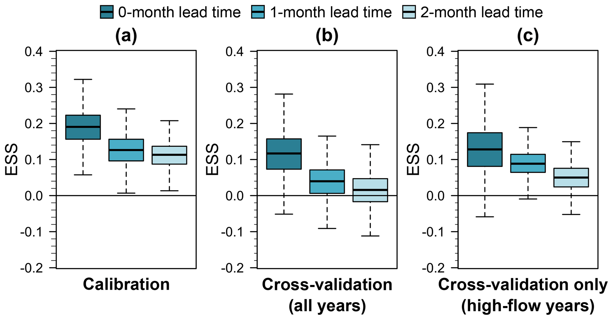
Figure 11 Energy skill score (ESS) distribution for different lead times from the (a) calibration, (b) leave‐1‐year‐out cross-validation, and (c) leave‐1‐year‐out cross-validation for extremes (60th percentile). Dark turquoise box plots denote a 0-month lead time, turquoise box plots a 1-month lead time, and light turquoise box plots a 2-month lead time. Higher values of the ESS indicate better model performance. Whiskers indicate the 95 % credible intervals, boxes the show interquartile range, and the horizontal lines inside the boxes show the median. Outliers are not displayed. All the models consider a Gaussian copula.

To assess at-site performance, we computed the continuous rank probability skill score (CRPSS; Hersbach, 2000; Gneiting and Raftery, 2007) at each gauge (see Fig. S4). As for the ESS, the CRPSS ranges from −∞ to 1, and its values have the same meaning (see Sect. 3.6). We obtained similar results compared to ESS (Fig. 11), with the exception of a few gauges for leave‐1‐year‐out cross-validation and leave‐1‐year‐out cross-validation for extremes, where the performance was poorer than the benchmark for the cross-validation.

Figure 12 shows the time series of the average projected spring maximum specific streamflow ensembles and the distributions of the Pearson correlation coefficient from the leave‐1‐year‐out cross-validation for the three lead times and the benchmark. Simulations relying on models with a copula show a similar variability and can capture observed values inside their ensemble's variability for all three lead times (Fig. 12a–b). The benchmark (Fig. 12d) cannot capture the observations since it converges to a stationary model, i.e., it gives the same projection for all years. There is a slight performance reduction for models with 1- and 2-month lead times compared to the 0-month lead time (Fig. 12e). The medians of the Pearson correlation coefficient for the three lead times vary between 0.37 and 0.5, while the median for the benchmark is close to −1. In addition, model performance for the calibration (see Fig. S5) is similar to the one of the cross-validation. This result indicates only small performance reductions for the projections and implies that the framework proposed could be useful for the early implementation of flood risk adaptation strategies each year.

Figure 12 Time series of average projected spring maximum specific streamflow (millimeters per day; hereafter mm d⁻¹), from the leave‐1‐year‐out cross-validation for a (a) 0-month lead time, (b) 1-month lead time, (c) 2-month lead time, (d)  the benchmark, and (e) the distributions of the Pearson correlation coefficient between the observed and the ensembles of the average projection spring maximum specific streamflow over all seven gauges for the different models. Blue and red points in panels (a)–(d) indicate when observations are captured (or not) by the ensemble's variability, respectively. Whiskers show the 95 % credible intervals, boxes the show interquartile range, and horizontal lines inside the boxes show the median. Outliers are not displayed. All lead time models consider a Gaussian copula.

5 Discussion

Compared to operational forecast models that consider short lead times and seasonal streamflow forecast models that are useful for reservoir operation with a focus on water availability during the dry season, the BHM proposed here has the following benefits:

• It allows for the consideration of potential climate change effects by modeling the margins in a nonstationary setting using suitable covariates.

• It allows one to capture the spatiotemporal dependence by including a Gaussian copula. Consequently, the spatial BHM captures observations that are not captured by the average projection of spring maximum specific streamflow of a BHM without a copula.

• It provides average projections of spring maximum specific streamflow for up to 2 months in advance by relying on the predictive skill of snow accumulated during the winter season.

The following question comes to mind: how can the proposed modeling framework be used to deliver interpretable seasonal average projections? It might be difficult for decision-makers to make decisions based on the average spring maximum specific streamflow over all seven gauges of the UCRB (see Fig. 12). To overcome this difficulty, we propose the provision of interpretable average projections of spring maximum specific streamflow by providing the first three quartiles of the ensembles along with some past streamflow values as a reference. Providing reference values can help one to make decisions about risk adaptation up to 2 months in advance. Reference values can be, e.g., the observed median specific streamflow for an average year without flood occurrence, the maximum observed specific streamflow on the record, or the lowest observed specific streamflow (threshold) that can cause flood occurrence. To find the threshold flow that can cause flood occurrence, we computed the ratio between the average maximum and average spring mean specific streamflow over all seven gauges of the UCRB. Then, we picked the average spring maximum specific streamflow value of the year with the highest ratio value, which corresponds to the threshold streamflow. The reason for this is that when the basin is drier (high ratio between peak runoff and total seasonal runoff), even if the peak streamflow is not so high, a flood can occur. Based on the lowest observed specific streamflow (threshold of q_thresh) that can trigger flood occurrence, we define a potential flooding alarm system. This system defines different flooding alarm levels by comparing the threshold against the first three quartiles (exceedance probability of q_25th, q_50th, and q_75th) of the average projections of spring maximum specific streamflow for the year analyzed. This potential flooding alarm system is shown in Fig. 13a. Thus, for each lead time, the flooding alarm is activated with a low risk of flooding if q_25th>q_thresh, a moderate risk of flooding if q_50th>q_thresh, or a high risk of flooding if q_25th>q_thresh. In all other cases, the alarm is not activated.

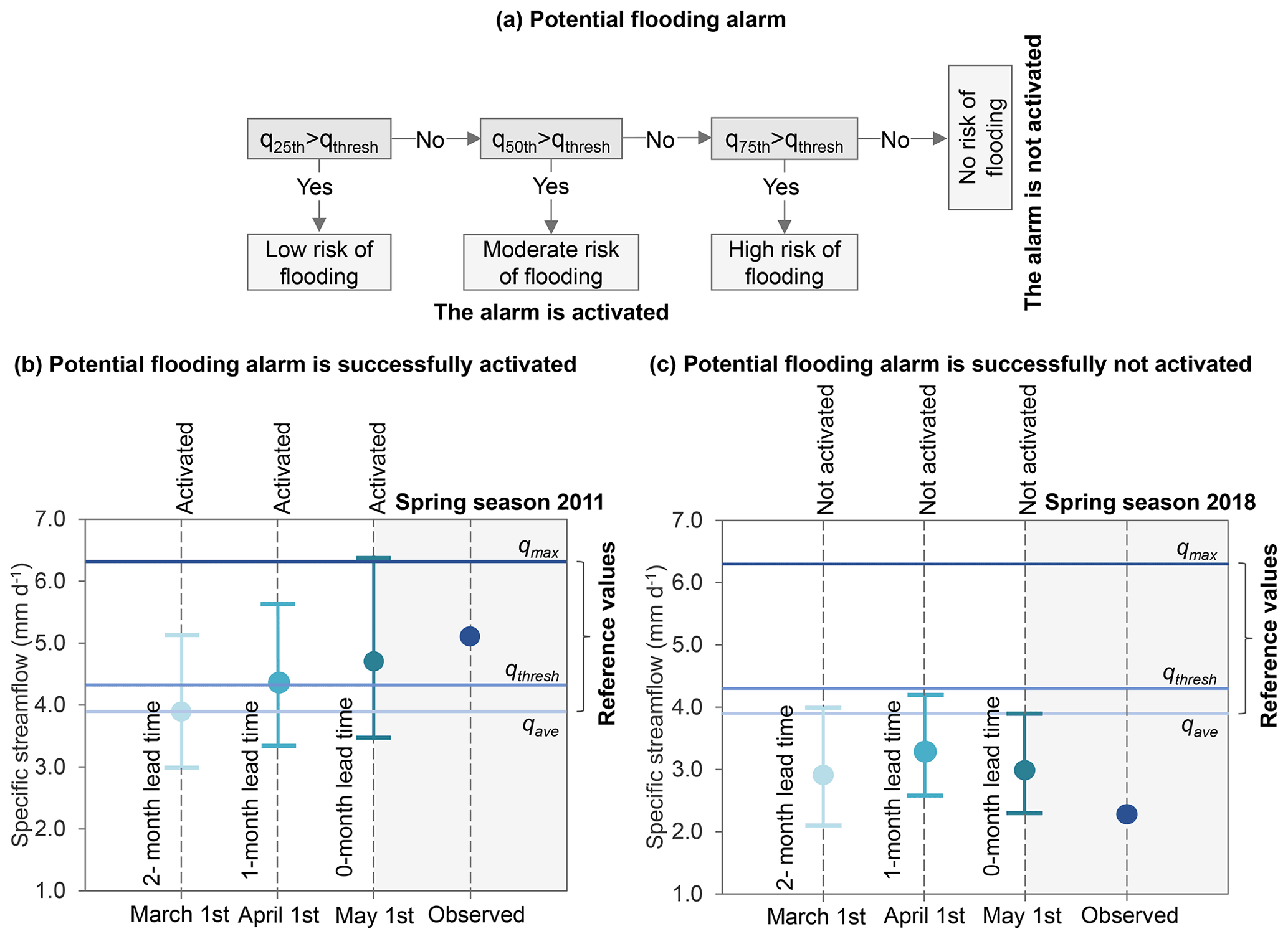
Figure 13 (a) Schematic of the potential flooding alarm system proposed. The flooding alarm is activated if q_25th>q_thresh (low risk of flooding), q_50th>q_thresh (moderate risk of flooding), or q_75th>q_thresh (high risk of flooding). Otherwise, the alarm is not activated. (b) Average projections of spring maximum specific streamflow of UCRB for 2011 when flooding is successfully activated, and (c) average projections of spring maximum specific streamflow of UCRB for 2018 when flooding is successfully not activated. Average projections at 0-, 1-, and 2-month lead times correspond to dark turquoise, turquoise, and light turquoise, respectively. The blue point corresponds to the observed specific streamflow for 2018, horizontal lines correspond to the observed highest specific streamflow (q_max; dark blue), observed flooding threshold specific streamflow (q_thresh; blue), and observed average specific streamflow (q_ave; light blue). For each lead time, the whiskers show the first and third quartile (q_25th and q_75th), and the points show the median or second quartile (q_50th).

To illustrate this system, Fig. 13b–c show examples of when the potential flooding alarm is successfully activated or not activated. Figure 13b presents the average projections of spring maximum specific streamflow of the UCRB for 2011 at three lead times (0–2 months), which were obtained from the leave‐1‐year‐out cross-validation, along with the three reference values mentioned above, and the observed value for 2011. It can be seen that, based on the average projections, the flooding alarm is activated with a low risk of flooding by 1 March (2-month lead time), a moderate risk of flooding by 1 April (1-month lead time), and a high risk of flooding by 1 May (0-month lead time). Thus, the flooding alarm is successfully activated before spring since the observed value for 2011 exceeded the threshold streamflow, and actually, flood impacts were documented in 2011 (Werner and Yeager, 2013). In addition, Fig. 13c shows the average projection of the spring maximum specific streamflow of the UCRB for 2018 when the flooding alarm is successfully not activated because the three quartiles for each lead time and the observed streamflow for 2018 are below the threshold streamflow.

The nonstationary and spatial BHM framework proposed here was applied to the UCRB using 3 d maxima. However, the framework is flexible and can be applied to other types of maxima, such as 1 d maxima, be implemented in other regions, be applied to other types of extremes such as droughts, or be used under future climate conditions. In order to apply the framework in another variable or region, the choice of covariates has to be reconsidered and potentially adjusted. In the application presented here, we only modeled the location parameter as nonstationary. If the framework is applied to another basin, this modeling choice has to be reconsidered. It is advisable, as a first step, to do an initial run of the model for defining which parameters should be considered nonstationary. If one wishes to apply the framework to predict another type of extreme such as low flows, one needs to reconsider distribution choice and to identify suitable covariates. In addition, the framework is not limited to projections; it can also be adapted for simulation purposes by considering real-time covariates. In addition, it can be easily adjusted such that it represents future climate conditions if future projections of the covariates are available. However, the predictive skill of the model fitted and applied to the UCRB may change under future climate conditions. The relative importance of snowmelt and precipitation in causing flood events may change in the future, with precipitation becoming relatively more important. Consequently, the model's predictive skill, which heavily relies on SWE as a covariate, might slightly decrease in future. However, in the case of headwater basins in mountainous regions, such as the one considered in this study, snowmelt will remain the dominant flood generation process in the future, as shown by climate change projections in the region (Safeeq et al., 2016). Under changing conditions, one may want to reconsider the covariate choice and test additional potentially skillful covariates such as specific ocean and atmosphere features that are expected to have a stronger relationship with the basin streamflow and extremes (e.g., Grantz et al., 2005; Regonda et al., 2006; Bracken et al., 2010). Although this framework can be applied to a more extensive stream gauges network, we do not recommend that since clusters of different streamflow behavior will develop as the size of the region of interest increases. In that case, it is more efficient to fit a model for each cluster than to fit a model for the entire region, which will be more computationally expensive. Fitting a model for each cluster allows for using different covariates for each cluster, which may help to provide more skillful estimates than the non-cluster case.

6 Summary and conclusions

In this study, we presented a Bayesian hierarchical model (BHM) to project seasonal streamflow extremes for several catchments in a river basin for several lead times. The streamflow extremes at a number of gauges in a basin are modeled using a Gaussian elliptical copula and generalized extreme value (GEV) margins with nonstationary parameters. These parameters are modeled as a linear function of suitable covariates from the previous season.

We applied this framework to project 3 d spring maximum (May–June) streamflow at seven gauges in the Upper Colorado River basin (UCRB) network, at 0-, 1-, and 2-month lead times. As potential covariates, we used indices of large-scale climate teleconnections, i.e., ENSO, AMO, and PDO, regional mean snow water equivalent, and temperature from the preceding winter season.

From the analysis of different models for a 0-month lead time, we conclude the following:

• The spatial average snow water equivalent (SASWE) accumulated during fall and spring is the most skillful predictor of spring season maximum streamflow across the UCRB.

• The increase in BHM performance is low when adding other climatic indices such as PDO.

• Including a copula in the BHM enables us to capture the spatiotemporal dependence of streamflow extremes, which is not fully possible with independent marginal models.

The comparative analysis for three different lead times revealed that increasing the lead time from 0 to 2 months only weakly decreases model skill. This finding implies that the framework proposed could be useful for the early implementation of flood risk adaptation and preparedness strategies. We propose an alternative to guide decision-making by providing the average projections of spring maximum specific streamflow as the first three quartiles of the ensembles of the average projection of the spring maximum specific streamflow along with past observed specific streamflow values as reference. Such a communication strategy could help decision-makers to implement adaptation strategies that address the spatial dimension of flooding.