the Creative Commons Attribution 4.0 License.
the Creative Commons Attribution 4.0 License.
 | 09 Mar 2022
Coupled effects of observation and parameter uncertainty on urban groundwater infrastructure decisions
Marina R. L. Mautner
Laura Foglia
Jonathan D. Herman
Urban groundwater management requires complex environmental models to represent interactions between hydrogeological processes and infrastructure systems. While the impacts of external uncertainties, such as climate and population growth, have been widely studied, there is limited understanding of how decision support is altered by endogenous uncertainties arising from model parameters and observations used for calibration. This study investigates (1) the importance of observation choice and parameter values on aquifer management objectives when controlling for model error and (2) how the relative performance of management alternatives varies when exposed to endogenous uncertainties, both individually and in combination. We use a spatially distributed groundwater model of the Valley of Mexico, where aquifer management alternatives include demand management, targeted infiltration, and wastewater reuse. The effects of uncertainty are evaluated using global sensitivity analysis, performance ranking of alternatives under a range of human–natural parameters, and identification of behavioral parameter sets filtered with an error metric calculated from varying subsets of observations. Results show that the parameters governing hydraulic conductivity and total water use in the basin have the greatest effect on management objectives. Error metrics (i.e., squared residuals of piezometric head) are not necessarily controlled by the same parameters as the head-based objectives needed for decision-making. Additionally, observational and parameter uncertainty each play a larger role in objective variation than the management alternatives themselves. Finally, coupled endogenous uncertainties have amplifying effects on decision-making, leading to larger variations in the ranking of management alternatives than each on their own. This study highlights how the uncertain parameters of a physically based model and their interactions with uncertain observations can affect water supply planning decisions in densely populated urban areas.
- Article
(4973 KB) - Full-text XML
- BibTeX
- EndNote


Groundwater resource planning and management requires increasingly complex models to represent interactions between hydrogeological and infrastructure systems to achieve sustainability (Megdal et al., 2015; Singh, 2014; Wada et al., 2017; Peters-Lidard et al., 2017). A key challenge for model-based decision support is understanding the influence of multiple sources of uncertainty on the choice of infrastructure alternatives. In particular, the role of external uncertainties, such as future climate, population, and land use change, have been investigated extensively in the systems analysis field (Hadka et al., 2015; Maier et al., 2016; Kwakkel and Haasnoot, 2019). Similar approaches have been applied in groundwater systems to analyze the combined effects of perturbations in external forcing (Dams et al., 2008, 2012; Mustafa et al., 2019; Fletcher et al., 2019). However, the endogenous uncertainties arising from physically based hydrologic and hydrogeologic models are often neglected in infrastructure planning studies, despite often influencing predictions as much or more than external drivers (Mendoza et al., 2016; Qiu et al., 2019; Herman et al., 2020). Furthermore, the effects of endogenous model uncertainties on model error may be different from their effects on the ranking of alternatives and, therefore, on decision making. This difference has been largely understudied and is the focus of this paper.
Physically based groundwater models can support infrastructure decisions by ranking alternatives according to their performance under stakeholder-defined management objectives. Global sensitivity analyses of the ranking of alternatives have generally focused on the influence of objective values and weights in multi-criteria decision models, without providing a physical basis for the determination of such variations (Hyde and Maier, 2006; Ganji et al., 2016). As a result, these decision models often do not account for uncertainty in hydrologic processes, leaving an opportunity to relate processes to the criteria values that are produced for a given management alternative. For example, Ravalico et al. (2009, 2010) analyze the effects of parameter changes on the optimal policy ranking by determining the minimum, median, and maximum parameter values that change the ranking of alternatives based on a single management objective; however, their implementation did not address model error. Specifically, none of the existing approaches explicitly evaluates the relationship between uncertain endogenous model characteristics used to determine model error and ranking of management alternatives for decision-making based on model output.
In hydrogeologic models, endogenous uncertainty is contributed by model parameters describing the natural and human components of the system and the set of historical observations used to calibrate or constrain the parameters (Moore and Doherty, 2005; Doherty and Simmons, 2013). Parameters provide the flexibility to represent complex systems on a broader scale and, in some cases, can encapsulate differences in model structure as well (Guillaume et al., 2016). The propagation and attribution of parameter uncertainty has been the topic of numerous hydrologic modeling studies, using a combination of uncertainty analysis and sensitivity analysis (Razavi et al., 2021; Pianosi et al., 2016), though generally without considering the influence of this uncertainty on model-based decision support (Jing et al., 2019) or only focusing on local sensitivity analyses (Tolley et al., 2019). Global sensitivity analysis in particular has seen growing usage with advances in computing power (Razavi and Gupta, 2015), including sensitivity varying over time and/or space (Herman et al., 2013; Şalap-Ayça and Jankowski, 2016; Reinecke et al., 2019; Zhang and Liu, 2021) and model structure (Mai et al., 2020). Observational uncertainty is typically also excluded, except in the case of inverse modeling (Refsgaard et al., 2007).
The choice of observations to support parameter identification is often complicated by a number of factors, including the temporal and spatial representation of the model area, data quantity and quality, and resolution of datasets that determine model structure with respect to observation locations (McMillan et al., 2018; Refsgaard et al., 2012; Lehr and Lischeid, 2020). This is especially true for groundwater modeling in urban environments, where infrastructure, monitoring practices, and pumping patterns can complicate groundwater data collection procedures meant to ensure accurate and repeatable results (Foster et al., 1998; Vázquez-Suñé et al., 2010; Bhaskar et al., 2016). Uncertainty in the selection of observations will alter the parameter calibration (Montanari and Di Baldassarre, 2013) and, in turn, the planning problem (Brunner et al., 2012). Similarly, Rojas et al. (2010) explore the availability and variety of observations in characterizing the choice of conceptual models in multimodel analysis, again focusing on effects on model error.
When developing groundwater models for planning purposes, calibration is often carried out by selecting a best parameter set by minimizing one or more error metrics while adjusting parameter values, using parameter sensitivity or expert evaluation to determine which parameters to adjust. Alternatively, some calibration frameworks use observations and the resulting behavioral model space of a selected error metric to refine the distribution of parameter values, rather than optimizing a single one (Wagener et al., 2003; Bárdossy, 2007; Beven, 2016). In such calibration frameworks, a behavioral parameter set comprises a sample of parameter sets from the behavioral model space through minimization of the error metric. A number of studies have focused on improving behavioral parameter set analysis by including regional datasets and expert knowledge, in addition to parameters and inputs (Kelleher et al., 2017), or evaluating sets that perform poorly with respect to a given error metric in addition to acceptable simulations (Reusser and Zehe, 2011). However, beyond prior studies of model error, there remains a need to understand the coupled effect of uncertainty in hydrogeologic model parameters and observations on the relative performance of decision alternatives (Razavi et al., 2021).
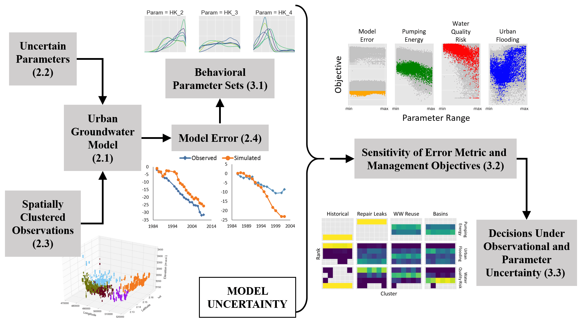
This study aims to evaluate the sensitivity of groundwater model error and decision-relevant management objectives to uncertain parameters and observations and to determine the effects of this coupled uncertainty on the infrastructure planning problem. The result is a planning-driven evaluation of uncertainty to support groundwater management, with the goals of identifying parameters to improve the accuracy of the hydrogeologic model and those that should be better constrained to support the selection of management alternatives. This is done through a combination of a global sensitivity analysis and a performance ranking under a range of human–natural parameters and with the identification of behavioral parameter sets based on multiple possible subsets of historical observations (Fig. 1). These diagnostic methods aim to evaluate the following two main consequences of these decision-relevant uncertainties: first, the importance of observation choice and parameter values on the absolute objective performance when controlling for model error, and second, how the relative performance of management alternatives varies when exposed to endogenous uncertainties, both individually and in combination. This approach exemplifies how the propagation of multiple endogenous uncertainties throughout the modeling process can ultimately affect the outcomes of regional groundwater supply planning.
This study focuses on the Mexico City Metropolitan Area to evaluate the effects of parameter and observation uncertainty on multi-objective groundwater modeling and decision-making. The Mexico City Metropolitan Area lies within the southwestern portion of the Valley of Mexico watershed, characterized by volcanic peaks surrounding a high plains basin (OCAVM, 2014). This paper uses a case study of the urban aquifer management problem in the Valley of Mexico, using a spatially distributed groundwater model adapted from prior work (Herrera-Zamarrón et al., 2005; Lopez-Alvis, 2014; Galán-Breth, 2018; Mautner et al., 2020). This type of complex, three-dimensional model is required to approximate the interactions between physical hydrogeologic properties and managed aquifer recharge interventions. This model complexity makes uncertainty analysis difficult, but it is also critical to understand how spatially and temporally aggregated management objectives vary across many parameter combinations.
2.1 Urban groundwater model
Table 1Model parameters and sampling ranges.
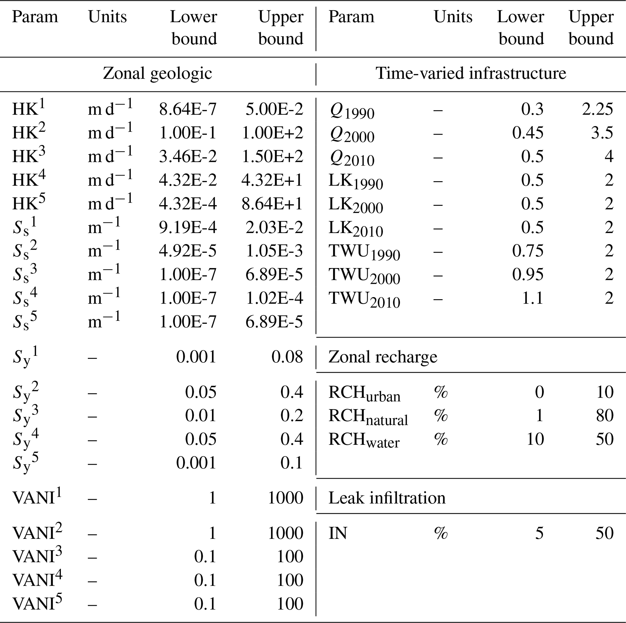
1 Lacustrine, 2 alluvial, 3 fractured basalt, 4 volcaniclastic, and 5 andesitic. Note: HK – horizontal hydraulic conductivity; Ss – specific storage; Sy – specific yield; VANI – vertical anisotropy of hydraulic conductivity; Q – urban pumping multiplier; LK – ratio of distribution leaks to estimated leaks using 1997 data; TWU – regional water use multiplier; RCH – recharge percentage for each land use type; IN – infiltration percentage for leaked water.
The Valley of Mexico model is written in Python, using the flopy package to preprocess data and run the model in MODFLOW, a widely used software which solves the groundwater flow equation (Bakker et al., 2019), as presented in Mautner et al. (2020). The following is a brief overview of the Valley of Mexico test case. A set of model parameters govern model representation of geologic setting, land use and land cover, and water resource infrastructure in Mexico City, including artificial and natural recharge, time-varied groundwater pumping, and heterogeneous subsurface characteristics (Table 1). This model covers an area of 84 km by 67 km on a 500×500 m spatial grid and the time period from 1984 to 2013. All model inflows and outflows are applied at a daily time step, varied according to a monthly stress period, meaning that data are provided at the monthly timescale, although data availability may cause some fluxes to vary at the annual or decadal timescale. The four management alternatives designed to increase groundwater recharge within the basin while avoiding flooding are drawn from Mautner et al. (2020). The alternatives were chosen based on conversations with local practitioners and previous modeling efforts. The alternatives are the implementation of spatially distributed infiltration basins, demand management through repair of leaks in the water supply network, injection of treated wastewater at existing wastewater treatment plants, and the status quo historical alternative.
Each alternative is then evaluated according to the following three aquifer management objectives: pumping energy use, water quality risk, and urban flood risk (Eqs. 1–3). The management objectives evaluated are drawn from Mautner et al. (2020) and modified to avoid outlier values that would occur when parameter combinations led to high quantities of model error that would affect the sensitivity analysis. The pumping energy objective (YE) is governed by the energy required to pump a daily quantity of groundwater (p) from the water table (h) to the ground surface (s) across all time periods (t) of varying length in days (d) and across all pumping wells (w), converted to kilowatt hours, using an efficiency and conversion term (ϵ). YE is calculated starting in the third year of the model period to avoid spin-up effects. In the Valley of Mexico, the lacustrine aquitard in the center of the valley serves as a barrier to contamination of the underlying productive alluvial aquifer, thereby ensuring that the hydraulic head remains above the confining layer and reduces water quality impacts in the long term. The water quality risk objective (YW) indicates the number of cells not meeting the groundwater levels below the confining lacustrine layer necessary to maintain water quality (l) divided by the total number of lacustrine cells in the model (L) during the time periods (t) in the last year of the model period. In conflict with the previous two objectives, certain parts of the city lie in areas that are affected by seasonal flooding resulting from medium-term groundwater mounding, which is particularly damaging in urban areas. To take into account these possible negative effects from increasing groundwater head within the valley, the urban flood risk (YF) is the sum of the urban area in cells with groundwater mounding (a) divided by the total urban area in the model (A) during the time periods (t) in the last year of the model period.
2.2 Uncertain parameters
The 33 model parameters include zonal geologic, time-varied infrastructure, zonal recharge, and infiltration characteristics (Table 1). There are four zonal geologic parameters for each of the five geologic formations, i.e., one parameter for each of the 3 decades during the model period for the total water use, ratio of urban to peri-urban pumping, and distribution system leak multiplier, a recharge percentage for each land use type, and an infiltration parameter for leaked water. Parameter ranges are adapted from Mautner et al. (2020), adding or adjusting maxima and minima where necessary based on the literature and physical relationships. The calibration carried out in Mautner et al. (2020) used a local sensitivity analysis in which some parameters were not assigned sampling ranges. In this study, a global sensitivity analysis is used, and thus, some combinations of parameter values had to be avoided based on the structure of the model (Table 1). For example, estimated pumping in the region is determined by subtracting historical non-pumping water source quantities from the total regional water use derived from the total water use multiplier (TWU), thus, the TWU must result in a regional water use greater than the historical non-pumping water sources. Similarly, the urban pumping multiplier (Q) acts on a historical dataset and must result in total pumping that is less than the estimated pumping determined by the combination of regional water use, historical other supply sources, and the TWU multiplier. The selected parameter ranges are shown in Table 1. Using these ranges, 100 000 unique parameter sets are generated using Latin hypercube sampling. Simulations for each of the management alternatives using the parameter sets were carried out on 296 processors over a total of 107 814 CPU hours. A single model run is of the order of 5 min, depending on the combination of parameters and the processor speed.
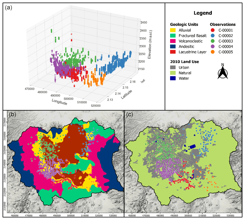
Figure 2(a) A 3-dimensional visualization of the five clusters of observations used in this study. (b) Observation clusters shown with the geologic formations within the model area. (c) Observation clusters shown with the land use types for the model period covering 2010.
2.3 Spatially clustered observations
Uncertainties introduced throughout the groundwater modeling process propagate through to decision-making, based on the simulated performance of management alternatives. Parameter uncertainty is reduced by calibration against observations. However, there is also error in, and uneven representation of the model area by, the observations used for calibration. Ideally, observation data can be filtered according to knowledge of collection methods, characteristics of monitoring wells, and distribution across the model area. However, increasingly, modelers face unwieldy and incomplete observation datasets that have greater degrees of freedom and limited or uncertain boundary conditions with which to calibrate models (Tiedeman et al., 2004; Tonkin et al., 2007; Hrachowitz et al., 2013; Nearing et al., 2021). These uncertainties can include a lack of data on the geologic formation boundaries,the placement and magnitude of cones of influence from pumping wells, and the effects of urban karst and land cover types on natural and artificial recharge near monitoring wells.
A set of 8181 observations from 676 monitoring wells is available for the area and time period of the urban groundwater model used in this study. Well observations vary from 1 to 29 data points per well over the 30-year model period, with a maximum of one observation per year. Multiple interacting uncertainties (e.g., land use, pumping wells, and geologic formations) can have unpredictable effects on the relevance of certain observations; thus, the observation uncertainty is represented in this study by separating the full set of observations into randomly selected and spatially distinct subsets of observations to act as proxies for incomplete historical records (Fig. 2). The full set was separated into five clusters, using centroid initialization of K-means clustering normalized within the 3-dimensional space of the set (Fig. 2), resulting in a total of six clusters when the full set is included as a control.
2.4 Model error
Doherty and Moore (2020) propose the selection of a decision-critical prediction when assimilating observed data into a model for calibration. In this model, the three groundwater planning objectives are based on various spatial and temporal aggregations of groundwater head values; thus, an error metric that assesses model agreement with piezometric head, the decision-critical prediction, through space and time was selected. As in Mautner et al. (2020), model error is captured by the sum of squared weighted residuals (SSWRs) between historical head observations (hobs, i) and simulated values (hsim, i), using weights (ω) determined in Lopez-Alvis (2014) and Galán-Breth (2018) as follows:
The model error is calculated under the status quo scenario to characterize model agreement with historical hydraulic head observations. Given the inclusion of multiple observations for a single well over time, the error metric captures both spatial and temporal variability in the hydraulic head. Higher values of this metric indicate poor model agreement with observations, with larger disagreements amplified in the metric as a result of the squared residual.
2.5 Parameter set selection
In complex systems with uncertain inputs, model processes can be difficult to parameterize and even more difficult to constrain. While perfect monitoring and representation is the ideal, in reality, simplifying assumptions must be calibrated to create models that can better inform policy and management. In such cases, it is common to have multiple viable parameter sets that produce simulations with acceptable or equivalent model error. Changes in the observations used to evaluate error can lead to differences in the behavioral parameter sets that are chosen as the best-performing simulations. Here, we calculate the error metric for each of the six observation clusters, inclusive of the full set of observations, and choose the 5 % best-performing parameter sets according to that metric. This gives a sample of 5000 parameter sets that perform relatively well with respect to the full sample of 100 000. We refer to these as the cluster behavioral parameter sets for each of the six observation clusters.
2.6 Sensitivity analysis
To better ensure robust management alternatives under uncertain model inputs, global sensitivity analysis has been increasingly explored as a decision support tool (Razavi et al., 2021). The sensitivity of the management objectives across the parameter space with respect to both management alternatives and cluster behavioral parameter sets indicates the variability in uncertainty with respect to individual physical model parameters. Using the cluster behavioral parameter sets, a global sensitivity analysis is performed using the delta moment-independent measure (δ) as follows (Borgonovo, 2007; Plischke et al., 2013):
where the moment independent sensitivity indicator of parameter Xi, with respect to the output Y (δi), represents the normalized expected shift in the distribution of Y as a function of μY and and the unconditional and conditional measures of Y, respectively. In this study, the parameters (Xi) are the 33 parameters shown in Table 1, and the outputs (Y) are the three management objectives described in Eqs. (1–3). This method was selected for two reasons. First, δ provides a better representation of sensitivity with respect to model structure when parameters are correlated, often true in complex human–natural systems (e.g., increased groundwater pumping during periods of reduced recharge and surface supplies from drought), when compared to variance-based methods (Borgonovo and Plischke, 2016). Second, the delta method does not require a specific structure of parameter samples, thus allowing for the sub-selection of 5000 samples from the initial set. By only evaluating objective sensitivity across the solution space of the cluster behavioral parameter sets rather than the entire solution space, we remove objective values of simulations that do not agree with observations and which have the potential to introduce further uncertainties. Parameter sensitivity is calculated for four model outputs, i.e., the error metric and three management objectives. A total of 72 sensitivity analyses on 33 parameters are performed across combinations of four alternatives, three objectives, and six cluster behavioral parameter sets resulting from filtering based on the error metric among each of the six observation clusters. The sensitivity analyses were performed on 72 processors over a total of 4.9 CPU hours.
2.7 Evaluation of decision uncertainty
To understand the extent to which uncertainty in observations and parameters can affect decision-making analyses, we compare alternative performance across cluster behavioral parameter sets. First, management alternatives are ranked within each objective for each of the parameter sets to view differences in the alternative ranking across the cluster behavioral parameter sets. We evaluate the model results to visualize changes in ranking according to three types of comparisons using sets of heat maps that summarize the ranking of the alternatives across all the parameter sets. The comparisons evaluated are as follows: (1) all three objectives across the observation cluster behavioral sets, (2) all three objectives for observation cluster behavioral set C-12345 across the range of the alluvial hydraulic conductivity parameter (HK2), and (3) the water quality objective (YW) across the observation cluster behavioral sets and parameter HK2, simultaneously.
In all three comparisons, the first step is to rank the alternatives according to the objective(s) from lowest (1) to highest (4) in each parameter set. Then, the ranking data for all the parameter sets in each comparison are summarized as follows:
-
Evaluate three objectives across observation cluster behavioral sets. This evaluation shows the count of rankings for each alternative. Each column (cluster) in each objective row will sum to 5000.
-
Evaluate three objectives for C-12345 across parameter HK2. The 5000 sample set is separated into 10 bins along the parameter value range from Table 1. The ranking count in each bin is divided by the total number of parameter samples in each bin to allow direct comparison across all bins. This is necessary because the distribution of behavioral parameters can be non-uniform. Each column (parameter value bin) in each objective row will sum to 100 % or null if there are no parameter sets in that bin.
-
Evaluate YW across the observation cluster behavioral sets and HK2, simultaneously. This is the same as in the previous comparison but for only the water quality objective. This is repeated for the remaining observation cluster behavioral sets (C-00001 to C-00005). Each column (parameter value bin) in each cluster row will sum to 100 % or null if there are no parameter sets in that bin.
Second, the difficulty of the decision was measured by evaluating the percent difference between the first and second ranked alternatives and between the first and worst ranked alternatives. The distribution of these differences indicate the relative performance between the alternatives, with a distribution concentrated among lower values indicating a more difficult decision because the relative differences between the objective measures of the options are smaller. While alternative ranking can provide some information on the relative performance of aquifer management alternatives with respect to each other, it does not provide information on the difference between the performance in each simulation. More importantly, by not knowing the range of objective values between the management alternatives in a given simulation, decision-makers might incorrectly infer the difficulty of a decision. For example, take the case of two simulations in which the performance in the urban flood risk objective of the historical, infiltration basin, wastewater reuse, and repair leaks alternatives are 1.5 %, 1.7 %, 1.8 %, and 2 %, respectively, in the first simulation, and 2 %, 15 %, 32 %, and 40 % in the second simulation. These two simulations may produce the same alternative ranking, i.e., historical (1), infiltration basins (2), wastewater reuse (3), and repair leaks (4). However, it is clear that second simulation produces a much easier decision than the first because the absolute and relative differences between the objective values are larger in the second simulation than in the first.
3.1 Cluster behavioral parameter sets
Figure 3 shows the kernel density estimations (KDEs) for the resulting parameter distributions when selecting the 5000 samples with the lowest error using each of the observation clusters (C-00001, C-00002, C-00003, C-00004, and C-00005) and the entire observation set (C-12345). The initial distribution (not shown) is uniform for all parameters. These distributions indicate the parameters that have the greatest influence on model error, defined here as those with the greatest deviation in distribution from the prior uniform distribution, namely the horizontal hydraulic conductivity (HK) parameters. The higher parameter values for the geologic characteristics (horizontal hydraulic conductivity – HK; specific storage – SS; specific yield – SY) of the alluvial formation (formation number 2) are preferentially represented in the low-error parameter sets. For hydraulic conductivity, this indicates that an alluvial formation (HK2) that allows for more rapid flow of groundwater, and thus greater dispersion of groundwater throughout the model area, results in a lower error. When combined with high values for flux parameters such as the total water use (TWU; governing groundwater pumping) and recharge (RCH), this could signal that these models avoid extreme mounding or drawdown that would increase model error. Similarly, the selection of a larger number of high values for specific storage (SS2) and specific yield (SY2) in the alluvial formation confirms that the selected parameters would tend to mitigate the effects of higher flux values. Alternatively, all distributions of the horizontal hydraulic conductivity show a concentration of lower values for the volcaniclastic formation (HK4). This indicates parameter values that encourage higher groundwater retention in the mountainous, volcaniclastic areas, which could be a result of observations in perched or mountainous regions having an outsized effect on the error metric.

Figure 3The distributions along the parameter ranges of the filtered samples, using the sum of squared error metric. The distributions are colored according to the observation cluster used to filter the dataset. The prior distribution (not shown) is uniform for all parameters. Parameter abbreviations are given in Table 1.
In terms of flux parameters, the total water use (TWU), the recharge percentage of the natural land use type (RCH2), and the leak (LK3) and pumping (Q3) multipliers for the third decade of the model period all show a small redistribution toward the extremes of the parameter ranges. The preference for lower values of total water use, particularly in the first decade (TWU1), could confirm that mitigated drawdown in the model leads to a lower error. At the same time, the slight tendency toward increased recharge in the natural land use type agrees with the tendency toward low hydraulic conductivity in the volcaniclastic formation that, combined, would indicate a preference for groundwater mounding along the model edges. Finally, the higher values for the leak parameter in the last decade of the model period (LK3) further confirms the preference for increased hydraulic head in the urban areas.
In isolation, these findings reveal information about the model representation and how to improve parameterizations to minimize error, given the existing observations. However, there are visible differences between the distributions of the parameter values from the various cluster behavioral parameter sets. This is particularly evident in the hydraulic conductivities of the alluvial (HK2), fractured basalt (HK3), and volcaniclastic formations (HK4). Behavioral parameter sets tend to focus on subranges of the horizontal hydraulic conductivity, depending on the subset of observations used to calculate the error metric, highlighting the importance of observational uncertainty on parameter identification.
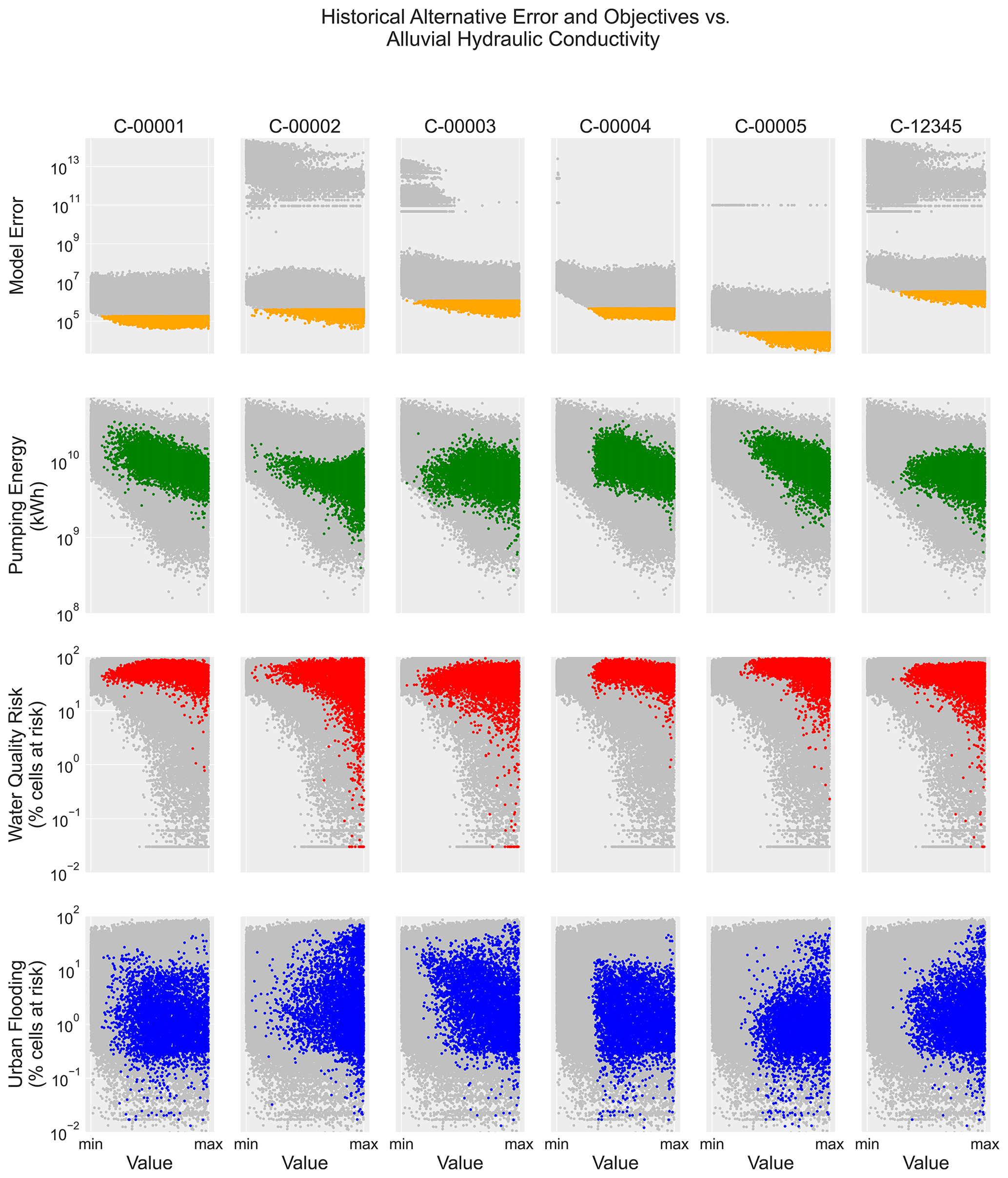
Figure 4A representative view of the four model output metrics for the historical alternative, plotted against the parameter range for the hydraulic conductivity of the alluvial formation (the most sensitive parameter from Fig. 3). These include the error metric (sum of squared weighted residuals; dimensionless), energy objective (kWh), water quality risk objective (percent of cells not meeting the objective), and urban flooding objective (percent of cells not meeting the objective). Gray points represent all parameter sets, while colors represent behavioral parameter sets meeting the error threshold.
Error reduction through parameter selection is an important consideration for model use. However, we are also interested in how management objectives produced by the model respond to uncertainty in model parameters. Figure 4 shows the error metric and the three management objectives for all parameter sets in gray and the behavioral parameter sets in color. Here we visualize how the choice of observation cluster affects the sample of parameter sets and, subsequently, the range of performance among the pumping energy (green), water quality risk (red), and urban flooding objectives (blue). This example yields noticeable differences between the observation cluster choices, while other parameters (Fig. S1) result in fairly uniform sampling across the parameter ranges, following Fig. 3. The three objectives are to be minimized; thus, in certain objectives, higher alluvial hydraulic conductivity (HK2) results in better performance, particularly for the energy and water quality objectives, while in the flooding objective the performance is more variable across the parameter range. This performance is not consistent across clusters for the alluvial hydraulic conductivity, indicating the impact of observational uncertainty on the performance evaluation of the system.
3.2 Sensitivity of error metric and management objectives
To better understand the effects of parameter values on management objectives, the moment-independent sensitivity measures, δ, are shown for the energy objective in Fig. 5 (see Fig. S2 for water quality risk and Fig. S3 for urban flooding risk). The value of δ can range from 0, indicating that the output is independent of the parameter in question, to 1. There is not a standard value for δ that is considered to be highly sensitive because parameter sensitivities should be evaluated in relation to each other and in the context of each case study. Based on the sensitivity values for this system, we consider a δ of roughly 0.2 and above to be highly sensitive. As in Fig. 4, the patterns of objective sensitivity to the parameters vary across the samples chosen using different observation clusters. However, in Fig. 5, we can also compare the sensitivity of the objectives across management alternatives. With a few exceptions, the sensitivities of the objectives across the alternatives within each cluster sample are fairly consistent. This suggests that the performance of the system with respect to the management objectives is minimally affected by the choice of alternative. This has two main implications. First, this could signify that the relative performance of the alternatives is similar across a range of parameter values and indicate that the decisions made are robust across many parameter combinations. Second, if decision-makers are using a sensitivity analysis to choose parameters for further study, then they can be relatively confident that the choice of parameters to monitor will not favor a given alternative. The most notable exception is the sensitivity of the pumping energy objective with respect to the leak multiplier (LK1, and to a lesser extent LK2 and LK3) for the repair leaks alternative. This is expected given the reliance of the leak repair alternative on the quantity of leaks present – essentially, more leaks available to be repaired indicates a larger water saving and, thus, a higher water table from which to pump to the ground surface.
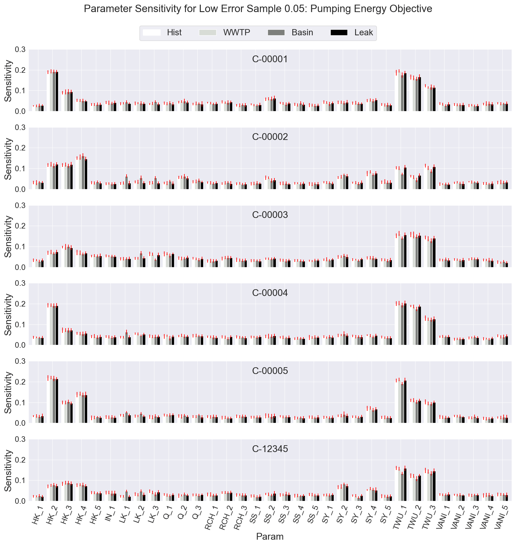
Figure 5δ sensitivity of the energy objective according to the 5000 filtered samples for the 33 model parameters (columns). The sensitivity is shown by cluster (rows) and by the four alternatives, from left to right (light to dark), i.e., historical, wastewater reuse, infiltration basins, and repair leaks. The bootstrapped 95 % confidence interval for each sensitivity value is shown as a red line.
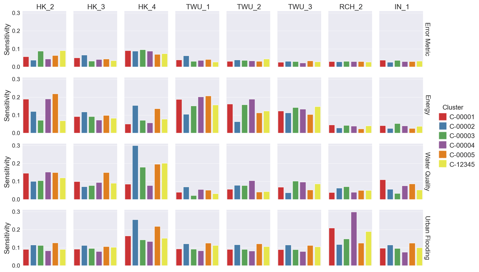
Figure 6δ sensitivity of the error metric and three management objectives (rows) according to the 5000 filtered samples for the eight model parameters (columns) with the largest differences in sensitivity between clusters for the historical management alternative. The sensitivity is shown by cluster in order, from left to right, i.e., C-00001, C-00002, C-00003, C-00004, C-00005, and C-12345.
It is also valuable to understand how the sensitivities of the three management objectives compare to those for the error metric. Many numerical groundwater models are constructed with a specific management purpose, but the model itself is calibrated to error metrics that represent available data, and these may not necessarily rely on the same mechanisms driving the performance of management alternatives. Figure 6 shows the δ values for the parameters with the largest differences in sensitivity between clusters. The sensitivities of the error metric across the filtered sample are relatively small because they include only the parameter sets with the lowest error. While the sensitivities of the error metric to the parameters are smaller overall than those of the objective values, the effects seen on the distributions in Fig. 3 are mirrored to some extent here, with slight increases in the sensitivity of the error metric to the horizontal hydraulic conductivity of the alluvial (HK2) and volcaniclastic (HK4) formations.
However, the patterns of the sensitivity of the error metric generally do not align with the patterns seen in the management objectives. Objectives are more or less sensitive to specific parameters, depending on the cluster behavioral parameter sets. For example, the sensitivity of all three management objectives to the volcaniclastic hydraulic conductivity (HK4) is largest for the C-00002 samples and is most pronounced for the water quality risk objective. Figure 4 shows that the parameter sets selected using the observation cluster C-00002 result in a much broader set of values for the hydraulic conductivity of the volcaniclastic formation than the other objective cluster samples, particularly for the water quality risk and urban flooding indicators. Similarly, samples C-00001 and C-00004 result in much higher sensitivities of the urban flooding objective to the recharge parameter of the natural land cover (RCH2).
Higher sensitivities for certain cluster behavioral parameter sets may indicate that the chosen observations do not properly constrain the model with respect to the given parameter, resulting in a number of non-unique solutions. Alternatively, higher sensitivities may occur when the spatial extent of the parameter and the management objective calculation are coincident, as in the case of the total water use parameters (TWU), which act upon the pumping wells, and the energy objective, which is calculated at the location of the pumping wells. Finally, the sensitivities are also affected by the physical processes governed by a given parameter, as in the case of the high sensitivity of the urban flooding objective to the recharge percentage parameter (RCH). Understanding which parameters contribute most to objective uncertainty indicates opportunities for data collection to improve model representation of those processes. The δ values show that uncertainties in the observations used in calibration can result in appreciable changes in the distribution of the performance in management objectives. These findings underline the importance of high quality, well-distributed, and diverse observation data for calibration. Additionally, decision-making often depends on the behavior of spatially and temporally aggregated indicators or objectives whose sensitivity to model parameters may or may not be aligned with the sensitivity of the error metric to those same parameters.
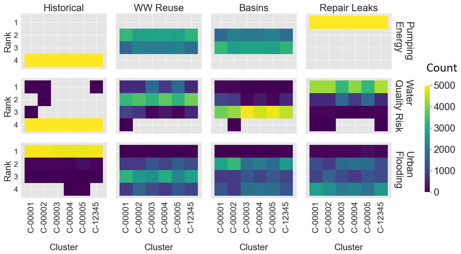
Figure 7Alternative performance across the observation cluster parameter sets shown as heat maps of the count of sets where the alternative performance was ranked from (1) best to (4) worst. Within each heat map, the rows are the rank, and the columns are the cluster behavioral parameter sets. The subplots are organized by the three management objectives (rows) and the aquifer management alternatives (columns).
3.3 Decisions under observational uncertainty
Parameter sensitivities provide information about improvements that can be made in the modeling and calibration process to reduce error. However, it is also important to understand how these uncertainties propagate into the decision-making process, particularly whether they contribute to changes in potential decisions informed by the simulation model. Figure 7 shows the relative performance of the aquifer management alternatives according to the cluster behavioral parameter set and management objective. In the heat maps, a lighter (yellow) color indicates more parameter sets where that alternative is ranked at that value, and a darker (purple) color indicates fewer parameter sets that are ranked at that values. If no parameter sets result in a given rank for that alternative, then the space is left gray.
For the pumping energy objective, the historical and repair leaks alternatives rank worst (4) and best (1), respectively, across all simulations in all parameter set samples, while the wastewater reuse and infiltration basin alternatives rank second and third almost evenly across the simulations. The wastewater reuse alternative ranks second slightly more often (lighter) in the pumping energy objective than the infiltration basin alternative, particularly in the C-00001 cluster behavioral parameter set and the full observation sample set (C-12345). In the water quality risk objective, the historical alternative ranks fourth across practically all the cluster behavioral parameter sets. Similarly, the infiltration basins alternative ranks third in almost all behavioral parameter sets. The first and second ranked alternatives, while less definitive, are still fairly clear, with the repair leaks alternative ranking first and the wastewater reuse alternative second across most of the cluster behavioral parameter sets. Here, C-00003 and C-00005 have less difference in the number of parameter sets where the repair leaks alternative ranks first and the wastewater reuse alternative second when compared to the other cluster behavioral parameter sets (C-00001, C-00002, C-00004, C-12345). Finally, in the urban flooding objective, the best-performing alternative is the historical alternative in the vast majority of the parameter sets across all cluster behavioral parameter sets. This is expected, given that the urban flooding objective measures groundwater mounding in the model, and since the remaining three management alternatives all increase recharge in the model, the status quo alternative experiences the least amount of mounding. However, the relative ranking between the other three alternatives is much less clear, particularly in the C-00003 and C-00005 cluster behavioral parameter sets.
Here it is apparent that the choice of observations by spatial clusters would have a minimal effect on decision-making, making this type of comparison of the alternatives robust across behavioral parameter sets chosen using observations from many different regions within the model area. This reveals the following two main points: first, the apparent agreement between sensitivities of performance to parameters across the alternatives may indicate the relative stability of the performance of alternatives across the cluster behavioral parameter sets, even though parameter sensitivities are not consistent across those same sets. Second, the comparison of rankings across the observational clusters may not capture the full interplay of absolute performance under observational uncertainties.
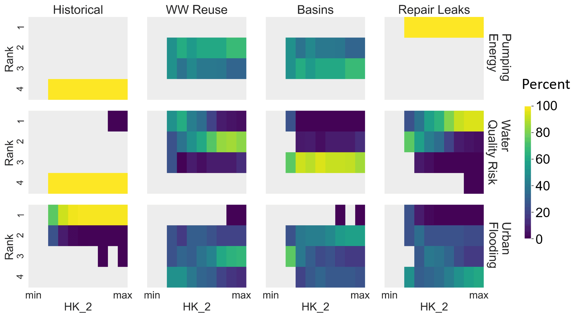
Figure 8Alternative performance across the parameter range of the alluvial hydraulic conductivity (one of the most sensitive parameters) shown as heat maps of the count of sets where the alternative performance was ranked from (1) best to (4) worst. Within each heat map, the rows are the rank, and the columns are the parameter value from minimum () to maximum (1.00×10²). The subplots are organized by the three management objectives (rows) and the aquifer management alternatives (columns).
Next, in Fig. 8, we compare the ranking across one of the most sensitive parameters, the hydraulic conductivity of the alluvial formation (HK2), looking only at the behavioral parameter sets chosen using the C-12345 (full) observation cluster. Similar to the comparison across observation clusters, the ranking of the management alternatives across the range of parameter values is stable for the pumping energy objective. The wastewater treatment and infiltration basin alternatives show a roughly even split between the second and third ranking. However, in the other two objectives, the ranking changes depending on the value of the alluvial hydraulic conductivity. This is particularly apparent in the water quality risk objective, although it also occurs to a lesser degree in the urban flooding objective. Notably, the repair leaks alternative ranks first in the water quality risk objective except at lower values of the parameter range, where the wastewater reuse objective is preferred. There are many competing factors that could contribute to this outcome. For example, lower hydraulic conductivity in the alluvial aquifer would indicate higher groundwater retention and could, thus, favor parameter sets with lower urban leak and total water use values to reduce model error by avoiding local mounding and cones of depression. In those cases, the wastewater treatment alternative would increase groundwater recharge more than the repair leak alternative and, thus, improve groundwater levels within the clay layer that influences water quality risk in the basin. Additionally, some of the fluctuations in the ranking result from the sample counts in each bin after the behavioral parameter set filtering. For example, the lowest bin in the water quality risk objective of the historical and infiltration basin alternatives shows a large difference because the sample count is low. In this case, a change in the bin size could change the relationship between the parameter values and the alternative ranking.
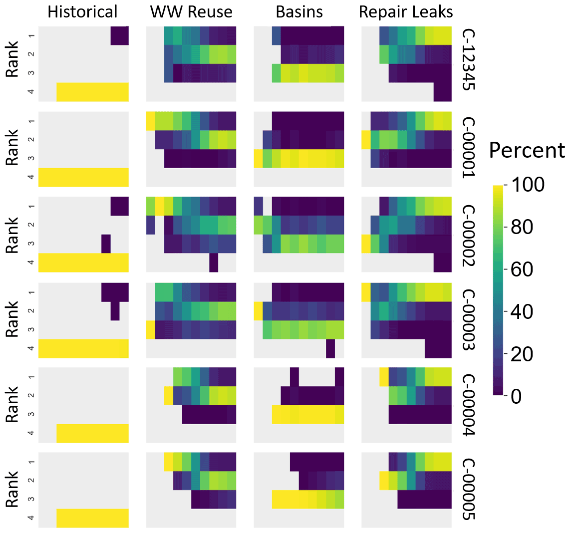
Figure 9Alternative performance in the water quality objective, shown as heat maps of the count of parameter sets, where the alternative performance was ranked from (1) best to (4) worst. Within each heat map, the rows are the rank, and the columns are the parameter value from minimum () to maximum (1.00×10²). The subplots are organized by the observation cluster used for the behavioral parameter set selection (rows) and the aquifer management alternatives (columns).
Finally, Fig. 9 shows the combined effects of the observation and parameter uncertainty on alternative performance in the water quality risk objective. Here it is apparent that the observation cluster choice has an effect on the ranking patterns of the management alternatives across the parameter range. While the pattern of favoring the wastewater reuse alternative at the lower alluvial hydraulic conductivity values and the repair leaks at the higher conductivity values is consistent across all the observation cluster behavioral parameter sets, the point along the parameter values at which this occurs changes between the clusters used to evaluate model error. There is even a case, at low alluvial hydraulic conductivity in the C-00002 set, where the wastewater reuse, infiltration basins, and repair leaks alternatives are ranked first, second, and third, respectively, in contrast with the findings from Fig. 7 and, to some extent, Fig. 8. This makes clear the importance of evaluating the coupled effects of multiple types of endogenous uncertainties on management outcomes in concert rather than in isolation.
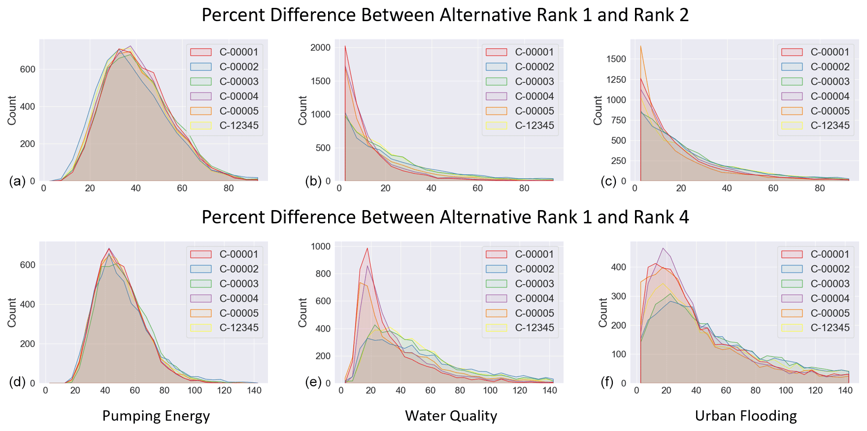
Figure 10The difficulty of the decision represented by the relative performance of the alternatives within the samples evaluated for each objective (columns). Panels (a)–(c) show the distribution of the percent difference in each sample between the first and second ranked alternatives within the cluster datasets. Panels (d)–(f) show the distribution of the percent difference in each sample between the first and fourth ranked alternatives within the cluster datasets.
To visualize the effects of the cluster behavioral parameter set on the difficulty of the decision, Fig. 10 shows the distributions of the percent differences between the first and second ranked alternatives in each sample (row 1) and between the best (first) and worst (fourth) ranked alternatives in each sample (row 2) for each cluster behavioral parameter set. In this figure, a distribution that is clustered near the origin of the graph indicates a more difficult decision because the percent difference between the objective values of each of the alternatives is smaller.
In the pumping energy objective, the minimal differences in the distributions confirm the conclusions, from Fig. 7, that the alternative rankings are not affected by which cluster behavioral parameter set was used for calibration. However, in the water quality risk objective, and to a lesser extent in the urban flooding objective, the cluster behavioral parameter set has an effect on the distribution of the percent difference between the first and second ranked alternatives and the best and worst ranked alternatives. In the water quality risk objective, C-00001, C-00004, and C-00005 show more instances of difficult decisions. These same cluster behavioral parameter sets also showed more difficult decisions in the urban flooding objective. This indicates that the availability of observational data could contribute to changes in the decision-making process when using the urban flooding and water quality risk objectives in this system.
3.4 Limitations and future work
Uncertainty analyses face limitations from model complexity and the sample size needed to capture multiple interacting forms of uncertainty. This study can be extended in several ways to address the challenge of propagating uncertainties throughout the groundwater infrastructure modeling and planning process. For example, this study did not consider multiple model structures and their effects on objective sensitivity and alternative ranking. Such changes could include varying representations of model geology and feedbacks after the implementation of management alternatives. Similarly, the use of observation clusters to reveal spatially dependent sensitivities may obscure the role of outlier observations on parameter sensitivity. Future work could identify the individual observations that contribute the most to sensitivity in each objective across the various parameters to understand better the limitations of the available observations, as has been achieved in other local sensitivity analysis approaches (Poeter et al., 2014; Matott, 2017; Tonkin et al., 2007).
As previous studies have applied space–time optimization for groundwater monitoring networks to reduce the variance of water quality estimates, future studies can apply similar techniques combined with the δ sensitivity measure of groundwater management objectives to determine optimal sampling locations. Additionally, uncertainty in the proper weighting of observations could be simulated using Monte Carlo selection of weights. Finally, clusters were chosen spatially in this study to simulate the over-representation of certain areas in monitoring; however, future research may compare clusters based on physical properties, such as land use and geologic formation, or other factors, such as the time period or the agency collecting the data. Similarly, bootstrapping or random selection instead of clustering could reveal the outsized influence of certain individual observations on parameter calibration and decision-making.
Additionally, while this study investigates parameter sensitivity and the effects of parameter uncertainty on ranking decisions, it does not explicitly quantify the relationship between the two. The results do not show a clear relationship between the magnitude of the sensitivity of the objectives to changes in the parameters. However, relative differences in the sensitivities of the objectives under different management alternatives may play a role in the alternative ranking. This relationship could be further investigated by developing a metric to capture the fluctuations in ranking driven by each parameter, which is then to be compared with the differences in sensitivity of a given parameter under each alternative. Similarly, while this study considers the impact of coupled uncertainties on three different management objectives, future work could implement a multi-objective approach evaluating Pareto optimality to consider all three objectives simultaneously.
Finally, the implementation of groundwater recharge alternatives could be modified to improve the accuracy of the simulations. One option would be to include costs of the management alternatives as either an additional objective or as a constraint to the implementation. Similarly, combinations of the various management alternatives or varying degrees of implementation may give further multi-objective benefits beyond those of each management alternative implemented individually.
In this study, we explore how observation and parameter uncertainty propagate through a hydrogeologic model to influence the ranking of decision alternatives. Using a global sensitivity analysis and an evaluation of aquifer management objectives across behavioral parameter sets filtered from a global sample, we evaluate how physical properties of the model and choice of observations for calibration can lead to variations in decision-relevant model outputs. We find that metrics that are generally used to determine predictive ability, such as the sum of squared weighted residuals, are not necessarily aligned with the decision-making applications for which models are applied. The management objective values in the behavioral parameter samples show a much greater range of sensitivity than those demonstrated by the model error. This underlines the importance of carrying through sensitivity analyses to the decision-making stage of the modeling process, beyond just the parameter calibration stage.
Additionally, results show that observational uncertainty plays a much larger role in the sensitivity of the objectives than the management alternatives themselves. This suggests that the performance of the system with respect to the management objectives is minimally affected by the choice of alternative when compared to the variability produced by endogenous model uncertainties. Under certain conditions, the relative performance of the alternatives under some of the objectives is consistent across many combinations of parameters and observation clusters – particularly for the pumping energy objective. This confirms that the performance of the demand management represented by the leak repair alternative is robust across many realizations of uncertainty.
The choice of observations shows a minimal effect on decision-making, with almost no differences in alternative ranking between the behavioral parameter sets. In contrast, the ranking of the leak repair and wastewater reuse alternatives showed fluctuations in ranking across the range of one of the most sensitive model parameters, i.e., the alluvial hydraulic conductivity. However, when combined with the parameter uncertainty, the observational uncertainty does contribute to greater fluctuations in alternative ranking. This makes clear the importance of evaluating the coupled effects of multiple types of endogenous uncertainties on management outcomes in concert, rather than in isolation.
Finally, the selection of alternatives becomes more or less difficult according to the relative performance of management objectives. Specifically, the distribution of the difficulty metric in each of the objectives changes based on the observation cluster used to select the behavioral parameter sets. These methods could be leveraged to determine which additional observations would help to more easily identify the best-performing alternative under multiple management objectives. This study highlights the importance of understanding how the uncertain parameters of a physical model and their interactions with the observations used to calibrate them can affect water supply planning decisions in densely populated urban areas.
Fig. A1 is an additional figure, similar to Fig. 4 in the main text, but with the x axis representing the vertical anisotropy of the hydraulic conductivity of the alluvial formation, a parameter that maintained uniform sampling across the parameter range.
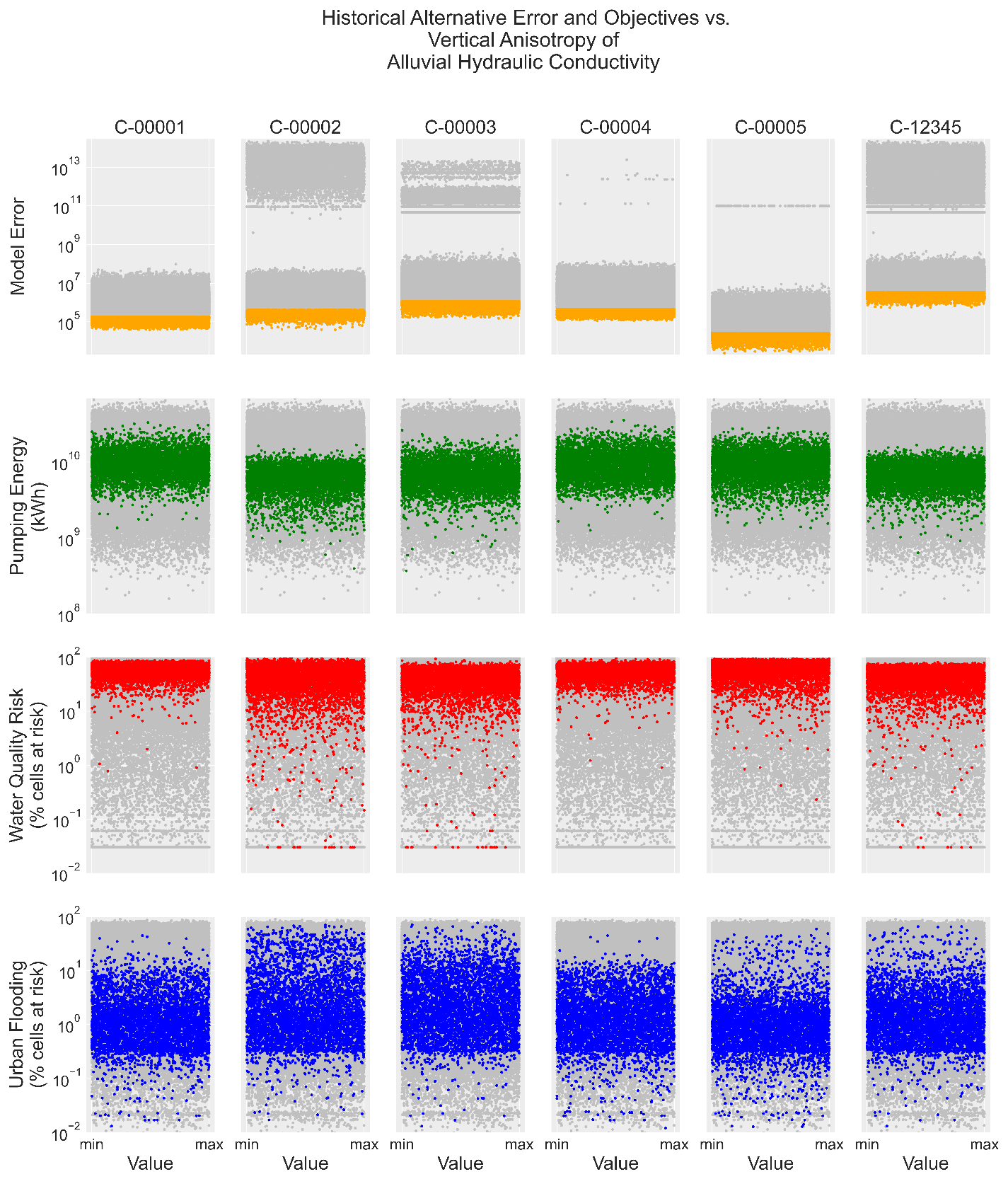
Figure A1A representative view of the four model output metrics for the historical alternative, plotted against the parameter range for the vertical anisotropy of the hydraulic conductivity of the alluvial formation. These include the error metric (sum of squared weighted residuals; dimensionless), energy objective (kWh), water quality risk objective (percent of cells not meeting the objective), and urban flooding objective (percent of cells not meeting the objective). Gray points represent all parameter sets, while colors represent behavioral parameter sets meeting the error threshold.
Figures A2 and A3 are additional figures, similar to Fig. 5 in the main text, but with the δ sensitivity values for the water quality risk objective and the urban flooding risk objective, respectively.
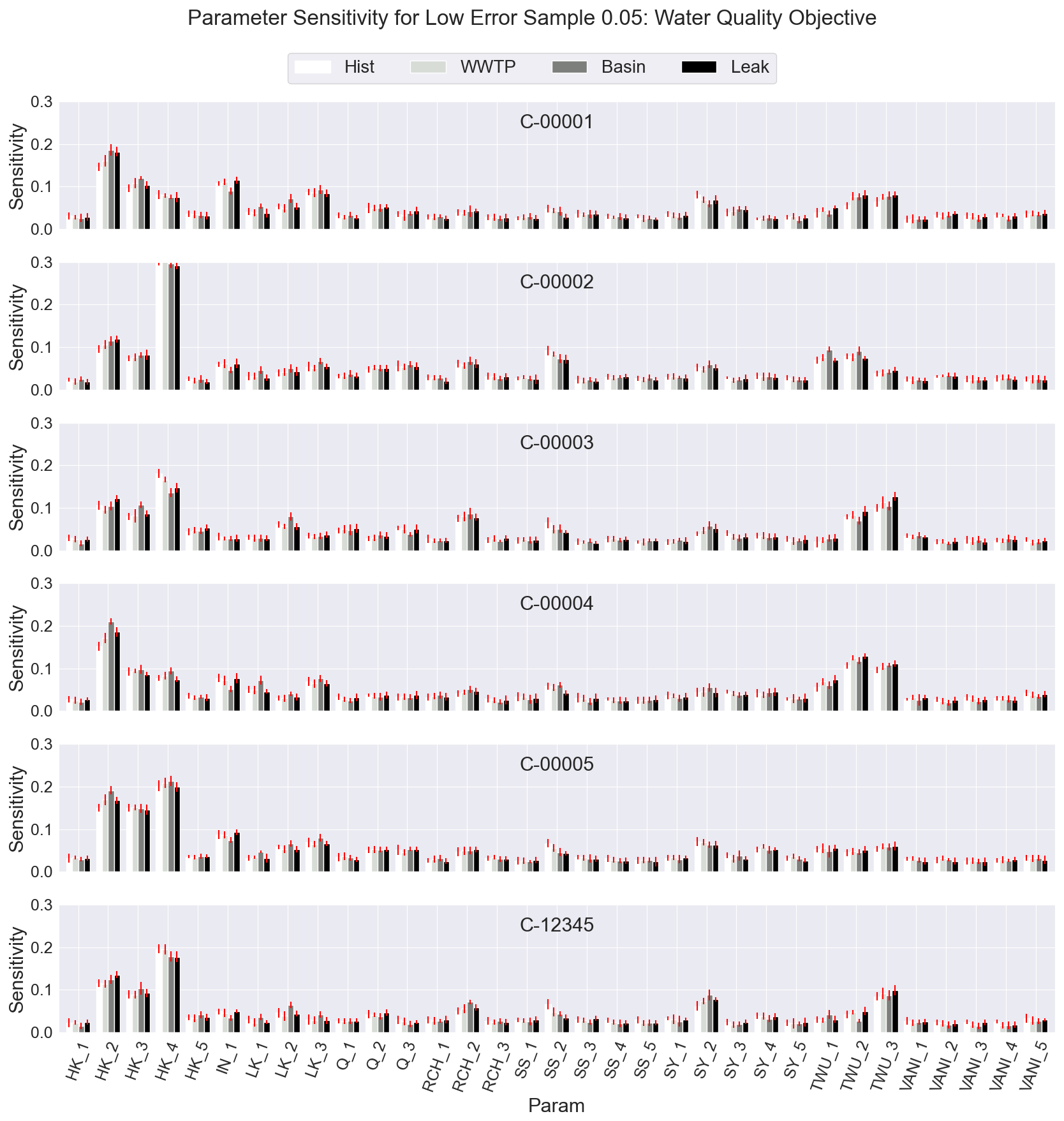
Figure A2δ sensitivity of the water quality risk objective according to the 5000 filtered samples for the 33 model parameters (columns). The sensitivity is shown by cluster (rows) and by the four alternatives from left to right (light to dark), i.e., historical, wastewater reuse, infiltration basins, and repair leaks.
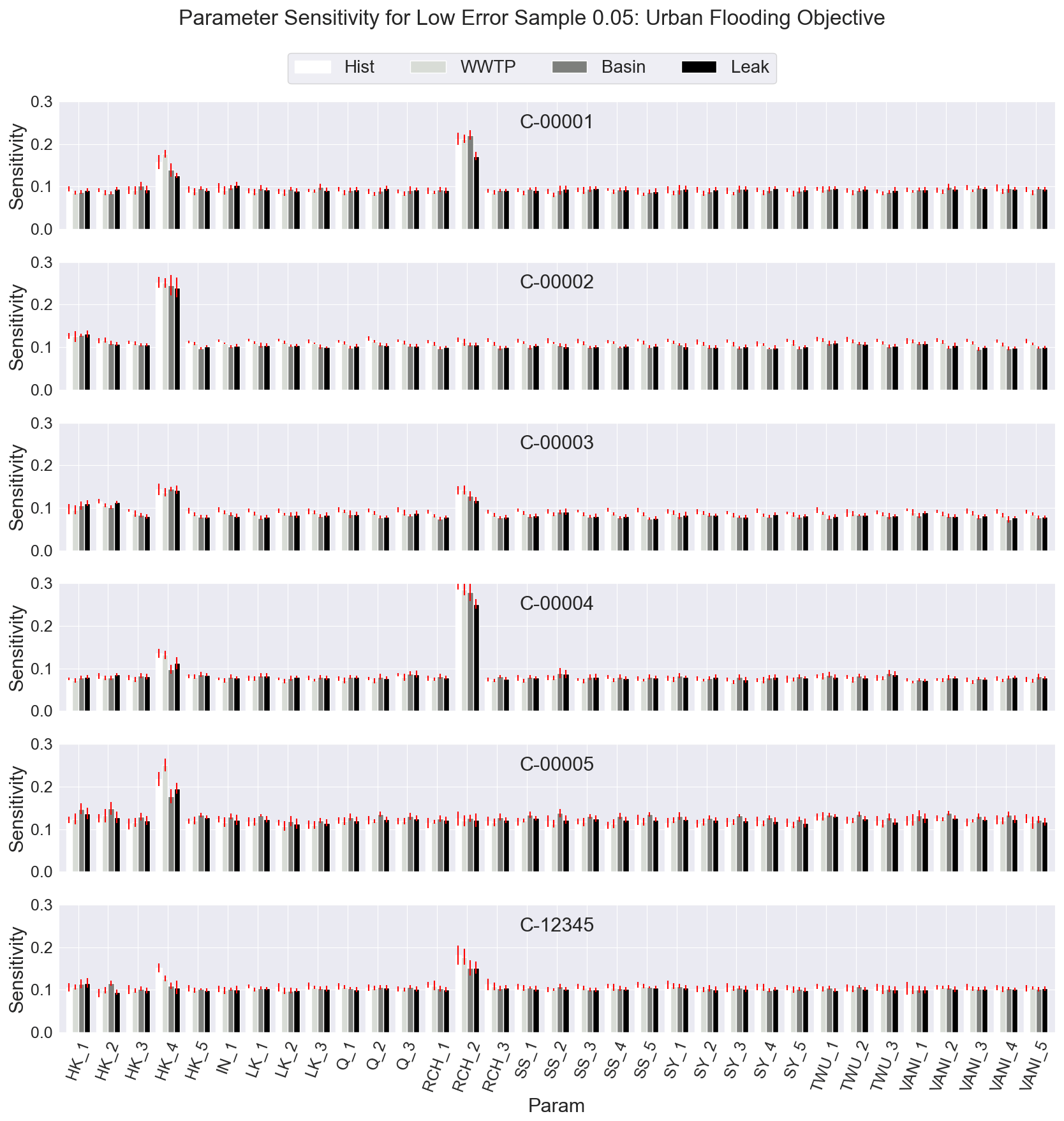
Figure A3δ sensitivity of the urban flooding risk objective according to the 5000 filtered samples for the 33 model parameters (columns). The sensitivity is shown by cluster (rows) and by the four alternatives from left to right (light to dark), i.e., historical, wastewater reuse, infiltration basins, and repair leaks.
The model, with input datasets, observations, results, and postprocessing scripts, is available in a GitHub repository at https://github.com/mrlmautner/UrbanGW/tree/sensitivityanalysis (last access: 10 February 2022) (https://doi.org/10.5281/zenodo.6039830; Mautner et al., 2022).
MRLM was responsible for the conceptualization, methodology, software, data curation, formal analysis, and writing the original draft. LF and JDH supervised and assisted with the conceptualization, review, and editing of the paper.
The contact author has declared that neither they nor their co-authors have any competing interests.
Publisher’s note: Copernicus Publications remains neutral with regard to jurisdictional claims in published maps and institutional affiliations.
This work has been supported in part by the Ford Foundation Predoctoral Fellowship Program of the National Academies of Science, Engineering, and Medicine. Research trips to Mexico City were funded in part by the University of California, Davis, Henry A. Jastro Graduate Research Award. We thank the Organismo de Cuencas: Aguas del Valle de México (OCAVM) of the National Water Commission (CONAGUA) of Mexico and the Instituto de Geofísica of the Universidad Nacional Autónoma de México (UNAM), for providing pumping and observation data, the conceptual groundwater model, and input on potential management alternatives.
This research has been supported by the Ford Foundation (Predoctoral Fellowship).
This paper was edited by Nadia Ursino and reviewed by two anonymous referees.
Bakker, M., Post, V., Hughes, J. D., Langevin, C. D., White, J. T., Leaf, A. T., Paulinski, S. R., Bellino, J. C., Morway, E. D., Toews, M. W., Larsen, J. D., Fienen, M. N., Starn, J. J., and Brakenhoff, D.: FloPy v3.2.12 — release candidate: U.S. Geological Survey Software Release, 31 May 2019 [code], https://doi.org/10.5066/F7BK19FH, 2019. a
Bárdossy, A.: Calibration of hydrological model parameters for ungauged catchments, Hydrol. Earth Syst. Sci., 11, 703–710, https://doi.org/10.5194/hess-11-703-2007, 2007. a
Beven, K.: Facets of uncertainty: epistemic uncertainty, non-stationarity, likelihood, hypothesis testing, and communication, Hydrolog. Sci. J., 61, 1652–1665, https://doi.org/10.1080/02626667.2015.1031761, 2016. a
Bhaskar, A. S., Beesley, L., Burns, M. J., Fletcher, T. D., Hamel, P., Oldham, C. E., and Roy, A. H.: Will it rise or will it fall? Managing the complex effects of urbanization on base flow, Freshw. Science, 35, 293–310, https://doi.org/10.1086/685084, 2016. a
Borgonovo, E.: A new uncertainty importance measure, Reliab. Eng. Syst. Safe, 92, 771–784, https://doi.org/10.1016/j.ress.2006.04.015, 2007. a
Borgonovo, E. and Plischke, E.: Sensitivity analysis: A review of recent advances, Eur. J. Oper. Res., 248, 869–887, https://doi.org/10.1016/j.ejor.2015.06.032, 2016. a
Brunner, P., Doherty, J., and Simmons, C. T.: Uncertainty assessment and implications for data acquisition in support of integrated hydrologic models, Water Resour. Res., 48, 1–18, https://doi.org/10.1029/2011WR011342, 2012. a
Dams, J., Woldeamlak, S. T., and Batelaan, O.: Predicting land-use change and its impact on the groundwater system of the Kleine Nete catchment, Belgium, Hydrol. Earth Syst. Sci., 12, 1369–1385, https://doi.org/10.5194/hess-12-1369-2008, 2008. a
Dams, J., Salvadore, E., Van Daele, T., Ntegeka, V., Willems, P., and Batelaan, O.: Spatio-temporal impact of climate change on the groundwater system, Hydrol. Earth Syst. Sci., 16, 1517–1531, https://doi.org/10.5194/hess-16-1517-2012, 2012. a
Doherty, J. and Moore, C.: Decision Support Modeling: Data Assimilation, Uncertainty Quantification, and Strategic Abstraction, Groundwater, 58, 327–337, https://doi.org/10.1111/gwat.12969, 2020. a
Doherty, J. and Simmons, C. T.: La modélisation de nappe comme support de décision: Réflexions sur un cadre conceptuel unifié, Hydrogeol. J., 21, 1531–1537, https://doi.org/10.1007/s10040-013-1027-7, 2013. a
Fletcher, S., Strzepek, K., Alsaati, A., and de Weck, O.: Learning and flexibility for water supply infrastructure planning under groundwater resource uncertainty, Environ. Res. Lett., 14, 114022, https://doi.org/10.1088/1748-9326/ab4664, 2019. a
Foster, S. S. D., Lawrence, A., and Morris, B.: Groundwater in urban development: assessing management needs and formulating policy strategies, no. 390 in World Bank technical paper series, World Bank, Washington, D.C, ISBN 978-0-8213-4072-1, 1998. a
Galán-Breth, R. I.: Modelación matemática de nitratos en el agua subterránea en la región Sur de la Ciudad de México, M.Sc. thesis, Instituto de Geofísica, Universidad Nacional Autónoma de México, México, 193 pp., 2018. a, b
Ganji, A., Maier, H. R., and Dandy, G. C.: A modified Sobol' sensitivity analysis method for decision-making in environmental problems, Environ. Modell. Softw., 75, 15–27, https://doi.org/10.1016/j.envsoft.2015.10.001, 2016. a
Guillaume, J. H. A., Hunt, R. J., Comunian, A., Blakers, R. S., and Fu, B.: Methods for Exploring Uncertainty in Groundwater Management Predictions, in: Integrated Groundwater Management, edited by: Jakeman, A. J., Barreteau, O., Hunt, R. J., Rinaudo, J. D., and Ross, A., 711–737, Springer International Publishing, https://doi.org/10.1007/978-3-319-23576-9_28, 2016. a
Hadka, D., Herman, J., Reed, P., and Keller, K.: An open source framework for many-objective robust decision making, Environ. Modell. Softw., 74, 114–129, https://doi.org/10.1016/j.envsoft.2015.07.014, 2015. a
Herman, J. D., Reed, P. M., and Wagener, T.: Time-varying sensitivity analysis clarifies the effects of watershed model formulation on model behavior, Water Resour. Res., 49, 1400–1414, https://doi.org/10.1002/wrcr.20124, 2013. a
Herman, J. D., Quinn, J. D., Steinschneider, S., Giuliani, M., and Fletcher, S.: Climate Adaptation as a Control Problem: Review and Perspectives on Dynamic Water Resources Planning Under Uncertainty, Water Resour. Res., 56, e24389, https://doi.org/10.1029/2019WR025502, 2020. a
Herrera-Zamarrón, G., Cardona-Benavides, A., González-Hita, L., Gutiérrez-Ojeda, C., Hernández-Calero, R., Hernández-García, G., Hernández-Laloth, N., López-Hernández, R. I., Martínez-Morales, M., Pita de la Paz, C., Sánchez-Díaz, L. F., Báez-Durán, J. A., Cruickshank-Villanueva, C., and Herrera-Revilla, I.: Estudio para obtener la disponibilidad del acuífero de la Zona Metropolitana de la Ciudad de México, Tech. Rep. Contract 06-CD-03-1O-0272-1-06, Secretaría del Medio Ambiente del Gobierno del Distrito Federal, Sistema de Aguas de la Ciudad de México (SACM), and Instituto Mexicano de Tecnología del Agua (IMTA), Mexico City, Internal Technical Report, Contract No. 06-CD-03-1O-0272-1-06, 2005. a
Hrachowitz, M., Savenije, H., Blöschl, G., McDonnell, J., Sivapalan, M., Pomeroy, J., Arheimer, B., Blume, T., Clark, M., Ehret, U., Fenicia, F., Freer, J., Gelfan, A., Gupta, H., Hughes, D., Hut, R., Montanari, A., Pande, S., Tetzlaff, D., Troch, P., Uhlenbrook, S., Wagener, T., Winsemius, H., Woods, R., Zehe, E., and Cudennec, C.: A decade of Predictions in Ungauged Basins (PUB) – a review, Hydrolog. Sci. J., 58, 1198–1255, https://doi.org/10.1080/02626667.2013.803183, 2013. a
Hyde, K. M. and Maier, H. R.: Distance-based and stochastic uncertainty analysis for multi-criteria decision analysis in Excel using Visual Basic for Applications, Environ. Modell. Softw., 21, 1695–1710, https://doi.org/10.1016/j.envsoft.2005.08.004, 2006. a
Jing, M., Heße, F., Kumar, R., Kolditz, O., Kalbacher, T., and Attinger, S.: Influence of input and parameter uncertainty on the prediction of catchment-scale groundwater travel time distributions, Hydrol. Earth Syst. Sci., 23, 171–190, https://doi.org/10.5194/hess-23-171-2019, 2019. a
Kelleher, C., McGlynn, B., and Wagener, T.: Characterizing and reducing equifinality by constraining a distributed catchment model with regional signatures, local observations, and process understanding, Hydrol. Earth Syst. Sci., 21, 3325–3352, https://doi.org/10.5194/hess-21-3325-2017, 2017. a
Kwakkel, J. H. and Haasnoot, M.: Supporting DMDU: A Taxonomy of Approaches and Tools, in: Decision Making under Deep Uncertainty, 355–374, Springer International Publishing, in: Decision Making under Deep Uncertainty, edited by: Marchau, V., Walker, W., Bloemen, P., and Popper, S., https://doi.org/10.1007/978-3-030-05252-2_15, 2019. a
Lehr, C. and Lischeid, G.: Efficient screening of groundwater head monitoring data for anthropogenic effects and measurement errors, Hydrol. Earth Syst. Sci., 24, 501–513, https://doi.org/10.5194/hess-24-501-2020, 2020. a
Lopez-Alvis, J.: Calibración de un modelo de flujo del Acuífero de la Zona Metropolitana de la Ciudad de México (AZMCM), Bachelor's thesis, Facultad de Ingeniería, Universidad Nacional Autónoma de México, México, 111 pp., 2014. a, b
Mai, J., Craig, J. R., and Tolson, B. A.: Simultaneously determining global sensitivities of model parameters and model structure, Hydrol. Earth Syst. Sci., 24, 5835–5858, https://doi.org/10.5194/hess-24-5835-2020, 2020. a
Maier, H., Guillaume, J., van Delden, H., Riddell, G., Haasnoot, M., and Kwakkel, J.: An uncertain future, deep uncertainty, scenarios, robustness and adaptation: How do they fit together?, Environ. Modell. Softw., 81, 154–164, https://doi.org/10.1016/j.envsoft.2016.03.014, 2016. a
Matott, L. S.: OSTRICH: an Optimization Software Tool, Documentation and User's Guide, Version 17.12.19, University at Buffalo Center for Computational Research, USA, 79 pp., 2017. a
Mautner, M. R. L., Foglia, L., and Herman, J. D.: mrlmautner/UrbanGW: Publication version (v2.1), Zenodo [code], https://doi.org/10.5281/zenodo.6039830, 2022. a
Mautner, M. R. L., Foglia, L., Herrera, G. S., Galán, R., and Herman, J. D.: Urban growth and groundwater sustainability: Evaluating spatially distributed recharge alternatives in the Mexico City Metropolitan Area, J. Hydrol., 586, 124909, https://doi.org/10.1016/j.jhydrol.2020.124909, 2020. a, b, c, d, e, f, g
McMillan, H. K., Westerberg, I. K., and Krueger, T.: Hydrological data uncertainty and its implications, WIREs Water, 5, 1–14, https://doi.org/10.1002/wat2.1319, 2018. a
Megdal, S. B., Gerlak, A. K., Varady, R. G., and Huang, L. Y.: Groundwater Governance in the United States: Common Priorities and Challenges, Groundwater, 53, 677–684, https://doi.org/10.1111/gwat.12294, 2015. a
Mendoza, P. A., Clark, M. P., Mizukami, N., Gutmann, E. D., Arnold, J. R., Brekke, L. D., and Rajagopalan, B.: How do hydrologic modeling decisions affect the portrayal of climate change impacts?, Hydrol. Process., 30, 1071–1095, https://doi.org/10.1002/hyp.10684, 2016. a
Montanari, A. and Di Baldassarre, G.: Data errors and hydrological modelling: The role of model structure to propagate observation uncertainty, Adv. Water Resour., 51, 498–504, https://doi.org/10.1016/j.advwatres.2012.09.007, 2013. a
Moore, C. and Doherty, J.: Role of the calibration process in reducing model predictive error, Water Resour. Res., 41, 1–14, https://doi.org/10.1029/2004WR003501, 2005. a
Mustafa, S. M. T., Hasan, M. M., Saha, A. K., Rannu, R. P., Van Uytven, E., Willems, P., and Huysmans, M.: Multi-model approach to quantify groundwater-level prediction uncertainty using an ensemble of global climate models and multiple abstraction scenarios, Hydrol. Earth Syst. Sci., 23, 2279–2303, https://doi.org/10.5194/hess-23-2279-2019, 2019. a
Nearing, G. S., Kratzert, F., Sampson, A. K., Pelissier, C. S., Klotz, D., Frame, J. M., Prieto, C., and Gupta, H. V.: What Role Does Hydrological Science Play in the Age of Machine Learning?, Water Resour. Res., 57, e2020WR028091, https://doi.org/10.1029/2020WR028091, 2021. a
OCAVM: Programa Hídrico Regional 2014–2018: Region Administrativo Hidrológico XIII, Aguas del Valle de México, Tech. rep., Comisión Nacional del Agua, Tlalpan, Mexico, D.F., Programa Hídrico Regional 2014–2018 Series, 2014. a
Peters-Lidard, C. D., Clark, M., Samaniego, L., Verhoest, N. E. C., van Emmerik, T., Uijlenhoet, R., Achieng, K., Franz, T. E., and Woods, R.: Scaling, similarity, and the fourth paradigm for hydrology, Hydrol. Earth Syst. Sci., 21, 3701–3713, https://doi.org/10.5194/hess-21-3701-2017, 2017. a
Pianosi, F., Beven, K., Freer, J., Hall, J. W., Rougier, J., Stephenson, D. B., and Wagener, T.: Sensitivity analysis of environmental models: A systematic review with practical workflow, Environ. Modell. Softw., 79, 214–232, https://doi.org/10.1016/j.envsoft.2016.02.008, 2016. a
Plischke, E., Borgonovo, E., and Smith, C. L.: Global sensitivity measures from given data, Eur. J. Oper. Res., 226, 536–550, https://doi.org/10.1016/j.ejor.2012.11.047, 2013. a
Poeter, E. P., Hill, M. C., Lu, D., Tiedeman, C., and Mehl, S. W.: UCODE_2014, with new capabilities to define parameters unique to predictions, calculate weights using simulated values, estimate parameters with SVD, evaluate uncertainty with MCMC, and more, Tech. rep., Integrated Groundwater Modeling Center (IGWMC), of the Colorado School of Mines, Report Number GWMI 2014-02, https://igwmc.mines.edu/ucode-2/ (last access: 7 March 2022), 2014. a
Qiu, J., Yang, Q., Zhang, X., Huang, M., Adam, J. C., and Malek, K.: Implications of water management representations for watershed hydrologic modeling in the Yakima River basin, Hydrol. Earth Syst. Sci., 23, 35–49, https://doi.org/10.5194/hess-23-35-2019, 2019. a
Ravalico, J. K., Maier, H. R., and Dandy, G. C.: Sensitivity analysis for decision-making using the MORE method-A Pareto approach, Reliab. Eng. Syst. Safe, 94, 1229–1237, https://doi.org/10.1016/j.ress.2009.01.009, 2009. a
Ravalico, J. K., Dandy, G. C., and Maier, H. R.: Management Option Rank Equivalence (MORE) – A new method of sensitivity analysis for decision-making, Environ. Modell. Softw., 25, 171–181, https://doi.org/10.1016/j.envsoft.2009.06.012, 2010. a
Razavi, S. and Gupta, H. V.: What do we mean by sensitivity analysis? the need for comprehensive characterization of “global” sensitivity in Earth and Environmental systems models, Water Resour. Res., 51, 3070–3092, https://doi.org/10.1002/2014WR016527, 2015. a
Razavi, S., Jakeman, A., Saltelli, A., Prieur, C., Iooss, B., Borgonovo, E., Plischke, E., Lo Piano, S., Iwanaga, T., Becker, W., Tarantola, S., Guillaume, J. H., Jakeman, J., Gupta, H., Melillo, N., Rabitti, G., Chabridon, V., Duan, Q., Sun, X., Smith, S., Sheikholeslami, R., Hosseini, N., Asadzadeh, M., Puy, A., Kucherenko, S., and Maier, H. R.: The Future of Sensitivity Analysis: An essential discipline for systems modeling and policy support, Environ. Modell. Softw., 137, 104954, https://doi.org/10.1016/j.envsoft.2020.104954, 2021. a, b, c
Refsgaard, J. C., van der Sluijs, J. P., Højberg, A. L., and Vanrolleghem, P. A.: Uncertainty in the environmental modelling process – A framework and guidance, Environ. Modell. Softw., 22, 1543–1556, https://doi.org/10.1016/j.envsoft.2007.02.004, 2007. a
Refsgaard, J. C., Christensen, S., Sonnenborg, T. O., Seifert, D., Højberg, A. L., and Troldborg, L.: Review of strategies for handling geological uncertainty in groundwater flow and transport modeling, Adv. Water Resour., 36, 36–50, https://doi.org/10.1016/j.advwatres.2011.04.006, 2012. a
Reinecke, R., Foglia, L., Mehl, S., Herman, J. D., Wachholz, A., Trautmann, T., and Döll, P.: Spatially distributed sensitivity of simulated global groundwater heads and flows to hydraulic conductivity, groundwater recharge, and surface water body parameterization, Hydrol. Earth Syst. Sci., 23, 4561–4582, https://doi.org/10.5194/hess-23-4561-2019, 2019. a
Reusser, D. E. and Zehe, E.: Inferring model structural deficits by analyzing temporal dynamics of model performance and parameter sensitivity, Water Resour. Res., 47, 1–15, https://doi.org/10.1029/2010WR009946, 2011. a
Rojas, R., Feyen, L., Batelaan, O., and Dassargues, A.: On the value of conditioning data to reduce conceptual model uncertainty in groundwater modeling, Water Resour. Res., 46, 1–20, https://doi.org/10.1029/2009WR008822, 2010. a
Şalap-Ayça, S. and Jankowski, P.: Integrating local multi-criteria evaluation with spatially explicit uncertainty-sensitivity analysis, Spat. Cogn. Comput., 16, 106–132, https://doi.org/10.1080/13875868.2015.1137578, 2016. a
Singh, A.: Groundwater resources management through the applications of simulation modeling: A review, Sci. Total Environ., 499, 414–423, https://doi.org/10.1016/j.scitotenv.2014.05.048, 2014. a
Tiedeman, C. R., Ely, D. M., Hill, M. C., and O'Brien, G. M.: A method for evaluating the importance of system state observations to model predictions, with application to the Death Valley regional groundwater flow system, Water Resour. Res., 40, 1–14, https://doi.org/10.1029/2004WR003313, 2004. a
Tolley, D., Foglia, L., and Harter, T.: Sensitivity Analysis and Calibration of an Integrated Hydrologic Model in an Irrigated Agricultural Basin With a Groundwater-Dependent Ecosystem, Water Resour. Res., 55, 7876–7901, https://doi.org/10.1029/2018WR024209, 2019. a
Tonkin, M. J., Tiedeman, C. R., Ely, D. M., and Hill, M. C.: OPR-PPR, a Computer Program for Assessing Data Importance to Model Predictions Using Linear Statistics, Techniques and Methods, p. 115, Technical report, OSTI identifier: 919524, Report no. TM 6-E2, United States Geological Survey, https://doi.org/10.2172/919524, 2007. a, b
Vázquez-Suñé, E., Carrera, J., Tubau, I., Sánchez-Vila, X., and Soler, A.: An approach to identify urban groundwater recharge, Hydrol. Earth Syst. Sci., 14, 2085–2097, https://doi.org/10.5194/hess-14-2085-2010, 2010. a
Wada, Y., Bierkens, M. F. P., de Roo, A., Dirmeyer, P. A., Famiglietti, J. S., Hanasaki, N., Konar, M., Liu, J., Müller Schmied, H., Oki, T., Pokhrel, Y., Sivapalan, M., Troy, T. J., van Dijk, A. I. J. M., van Emmerik, T., Van Huijgevoort, M. H. J., Van Lanen, H. A. J., Vörösmarty, C. J., Wanders, N., and Wheater, H.: Human–water interface in hydrological modelling: current status and future directions, Hydrol. Earth Syst. Sci., 21, 4169–4193, https://doi.org/10.5194/hess-21-4169-2017, 2017. a
Wagener, T., McIntyre, N., Lees, M. J., Wheater, H. S., and Gupta, H. V.: Towards reduced uncertainty in conceptual rainfall-runoff modelling: dynamic identifiability analysis, Hydrol. Process., 17, 455–476, https://doi.org/10.1002/hyp.1135, 2003. a
Zhang, X. and Liu, P.: A time-varying parameter estimation approach using split-sample calibration based on dynamic programming, Hydrol. Earth Syst. Sci., 25, 711–733, https://doi.org/10.5194/hess-25-711-2021, 2021. a