the Creative Commons Attribution 4.0 License.
the Creative Commons Attribution 4.0 License.
 | 09 Mar 2022
Probabilistic modelling of the inherent field-level pesticide pollution risk in a small drinking water catchment using spatial Bayesian belief networks
Mads Troldborg
Zisis Gagkas
Andy Vinten
Allan Lilly
Miriam Glendell
Pesticides are contaminants of priority concern that continue to present a significant risk to drinking water quality. While pollution mitigation in catchment systems is considered a cost-effective alternative to costly drinking water treatment, the effectiveness of pollution mitigation measures is uncertain and needs to be able to consider local biophysical, agronomic, and social aspects. We developed a probabilistic decision support tool (DST) based on spatial Bayesian belief networks (BBNs) that simulates inherent pesticide leaching risk to ground- and surface water quality to inform field-level pesticide mitigation strategies in a small (3.1 km2) drinking water catchment with limited observational data. The DST accounts for the spatial heterogeneity in soil properties, topographic connectivity, and agronomic practices; the temporal variability of climatic and hydrological processes; and uncertainties related to pesticide properties and the effectiveness of management interventions. The rate of pesticide loss via overland flow and leaching to groundwater and the resulting risk of exceeding a regulatory threshold for drinking water was simulated for five active ingredients. Risk factors included climate and hydrology (e.g. temperature, rainfall, evapotranspiration, and overland and subsurface flow), soil properties (e.g. texture, organic matter content, and hydrological properties), topography (e.g. slope and distance to surface water/depth to groundwater), land cover and agronomic practices, and pesticide properties and usage. The effectiveness of mitigation measures such as the delayed timing of pesticide application; a 10 %, 25 %, or 50 % reduction in the application rate; field buffers; and the presence/absence of soil pan on risk reduction were evaluated. Sensitivity analysis identified the month of application, the land use, the presence of buffers, the field slope, and the distance as the most important risk factors, alongside several additional influential variables. The pesticide pollution risk from surface water runoff showed clear spatial variability across the study catchment, whereas the groundwater leaching risk was uniformly low, with the exception of prosulfocarb. Combined interventions of a 50 % reduced pesticide application rate, management of the plough pan, delayed application timing, and field buffer installation notably reduced the probability of a high risk of overland runoff and groundwater leaching, with individual measures having a smaller impact. The graphical nature of BBNs facilitated interactive model development and evaluation with stakeholders to build model credibility, while the ability to integrate diverse data sources allowed a dynamic field-scale assessment of “critical source areas” of pesticide pollution in time and space in a data-scarce catchment, with explicit representation of uncertainties.
- Article
(23020 KB) - Full-text XML
- BibTeX
- EndNote


Diffuse pesticide pollution continues to represent a significant risk to surface and drinking water quality worldwide (Villamizar et al., 2020). European Union legislation – the Water Framework Directive (WFD; European Commission, 2000), the related Drinking Water Directive (DWD; European Commission, 1998), and the Groundwater Directive (GWD; European Commission, 2006) – require that the concentration of individual pesticides in drinking water must not exceed 0.1 µg L−1, and the total concentration of all pesticides must be below 0.5 µg L−1. Article 7 of the WFD promotes a “prevention-led” approach to DWD compliance, prioritising pollution prevention at the source rather than costly drinking water treatment. Therefore, catchment management schemes are now widely adopted by policy makers and water companies to mitigate diffuse pollution by pesticides (and other pollutants) and to improve the raw water quality prior to treatment. However, the effectiveness of such diffuse pollution mitigation measures is uncertain due to the heterogeneous nature of catchment systems; hence, catchment management needs to be targeted to consider local biophysical, agronomic, and social aspects (Okumah et al., 2018). To select and prioritise cost-effective interventions, it is essential to identify and map “high risk” areas, often referred to as “critical source areas” (CSAs), i.e. those areas within a catchment that contribute disproportionately large amounts of pollutants to a given water quality problem (Doody et al., 2012; Reaney et al., 2019).
Modelling approaches are commonly used to identify diffuse pesticide pollution risk areas and to help evaluate the effectiveness of mitigation strategies. While process-based distributed models, such as the Soil and Water Assessment Tool (SWAT), have been widely used to simulate the transport, fate, and risks of pesticides at the catchment scale as well as to evaluate the effectiveness of interventions (Babaei et al., 2019; Villamizar et al., 2020; Wang et al., 2019), their application is computationally costly and often hindered by a lack of monitoring data for model calibration and validation. Therefore, various spatial index models have been developed to evaluate the intrinsic vulnerability and risk from pesticide pollution at a range of scales (Kookana et al., 2005; Stenemo et al., 2007; Worrall and Kolpin, 2003). The simplest index-based methods assign scores and weights to a set of spatially distributed indicators (e.g. soil media, recharge rate, and depth to groundwater and contaminant properties), which are then combined into an overall risk index, typically within a geographic information system (GIS) environment. An example of such index-based method is the DRASTIC system (Aller et al., 1987), which has been widely used for groundwater vulnerability mapping and for identifying areas most at risk to pollutant leaching. DRASTIC only considers geological and hydrogeological factors but ignores the specific nature of the contaminant (s); therefore, it is classed as an intrinsic vulnerability method. Several modifications and methods similar to DRASTIC exist in the literature, many of which aim to provide specific vulnerability maps, where the contaminant source and behaviour are also accounted for (Duttagupta et al., 2020; Nobre et al., 2007; Saha and Alam, 2014). Other studies have used simplified 1D solute transport models to develop indices and rankings of potential pesticide leaching (Gustafson, 1989; Jury et al., 1987; Stenemo et al., 2007), while other methods such as the SCIMAP modelling framework (Lane et al., 2009; Reaney et al., 2011) use digital elevation models to derive spatial patterns of relative potential erosion and hydrological connectivity to identify possible critical source areas for diffuse pollution risk.
While index-based vulnerability methods are useful for initial screening purposes, they also have several limitations. Index-based methods do not account for uncertainties in model parameters and complex processes, and they lack the probabilistic integration of lines of evidence (Carriger et al., 2016; Carriger and Newman, 2012). In addition, the scores and weights are typically assigned subjectively, and different scoring systems can, therefore, provide substantially different results. Finally, index-based methods usually do not account for actual concentration data, and poor correlations between vulnerable areas and field concentration measurements have been reported (Worrall and Kolpin, 2003).
To address the first two shortcoming, we developed a probabilistic decision support tool (DST) using spatial Bayesian belief networks (BBNs) to inform field-level pesticide mitigation strategies in a small (3.5 km2) drinking water catchment with limited observational data. BBNs are probabilistic graph-based models that allow one to integrate various information sources, including different types of data, literature, and expert opinion into a single modelling framework, thereby maximising the use of both available knowledge and data (Carriger et al., 2016; Carriger and Newman, 2012). In BBNs, model variables and their causal relationships are represented as “nodes” and “arcs” in a so-called directed acyclic graph (DAG) (i.e. a graph that has no feedback loops). The graphical nature of a BBN lends itself to collaborative model co-construction with experts and stakeholders and helps to build model credibility. A major advantage of the BBN approach is that it allows one to carry out probabilistic inference based on (uncertain) evidence. Probabilistic inference is simply the task of calculating the posterior probability distribution of the BBN given the available observations, and it can be both predictive (i.e. reasoning from new observations of causes to new beliefs about the effects) and diagnostic (i.e. reasoning from observed effects to updated beliefs about causes).
The use of BBNs has gained increasing popularity in environmental modelling and risk assessment (Aguilera et al., 2011; Kaikkonen et al., 2020), with examples including pesticide risk management (Carriger and Newman, 2012; Henriksen et al., 2007) and probabilistic assessments of pesticide exposure and effects (Mentzel et al., 2021). While the integration of Bayesian networks with GIS in environmental risk assessment has also been growing steadily over recent years (Moe et al., 2021), spatial BBN has currently only been used for pesticide risk modelling on a single occasion to assess pesticide runoff risk at a basin scale across France (Piffady et al., 2020). To our knowledge, the present study provides the first application of spatial BBN for probabilistic field-level assessment of intrinsic pesticide pollution risk from critical source areas at a monthly resolution.
The aim of this research was to examine the spatial variability of risk factors within an uncertainty framework to better inform field-level targeting of management interventions in a small drinking water catchment with limited available data. Specifically, we sought to answer the following questions:
-
Can we characterise the spatial and temporal variability of pesticide pollution risk from groundwater leaching and overland flow in a data-sparse catchment?
-
Which factors are most influential on intrinsic pesticide pollution risk?
-
What is the effectiveness of available management interventions with respect to pesticide risk reduction?
2.1 Study site
The island of Jersey (ca. 117 km2; 49.2138∘ N, 2.1358∘ W), the largest in the English Channel group, comprises a plateau with an elevation 60–120 m above sea level (Robins and Smedley, 1998). The climate on Jersey is oceanic, the average temperature ranges from 6 ∘C in winter to 18 ∘C in summer, and the mean annual rainfall is around 900 mm. A shallow, fractured bedrock aquifer underlies most of the island, with a generally shallow depth to the water table increasing to 10–30 m beneath higher ground. For the most part, groundwater storage and transport is shallow and within the top 25 m of the saturated rock (Robins and Smedley, 1998). Bedrock is Precambrian to Cambrian–Ordovician. The western central part of the island is mostly underlain by the oldest rocks belonging to the Jersey Shale Formation, while a volcanic formation occupies much of the east. Superficial deposits include wind-blown sand, loess, and alluvium (Robins and Smedley, 1991).
Historically, water resources across the island of Jersey have been vulnerable to nitrate and pesticide pollution, particularly during the growing season when concentrations in untreated water can exceed regulatory drinking water quality levels. This can adversely affect the raw water quality within impounding reservoirs, requiring the water company to undertake a series of mitigation measures at the treatment works to avoid breaches in the treated water supply. The small size of the island means that land use across the island is dominated by intensive agriculture, primarily potato and dairy farming. The cultivation of the Jersey Royal potato takes place during the growing season from January to May. There is very little crop rotation and, accordingly, the potato crop is grown with the support of synthetic fertilisers and pesticides (herbicides, fungicides, and nematicides).
This study focused on the Val de la Mare (VDLM) catchment (3.1 km2) in the south-west of Jersey, which feeds into the VDLM reservoir, the second largest reservoir in Jersey, constructed in 1962. The reservoir holds up to 938 700 m3 of untreated water, enough to supply Jersey with water for approximately 5 weeks. Water feeds into the reservoir from within the catchment area as well as from neighbouring catchments and a desalination plant (when it is in operation). The water quality in the VDLM reservoir is vulnerable to pesticide pollution, with pesticide concentrations often exceeding the regulatory drinking water quality levels of 0.1 µg L1 for individual pesticides and 0.5 µg L−1 for the total pesticide concentration (European Commission, 1998).
To evaluate the spatial and temporal variability of the intrinsic pesticide pollution risk from critical source areas within the VDLM study catchment, we have developed a probabilistic model based on spatial Bayesian belief networks (BBNs). The data and information used to inform the model development are presented in Sect. 2.2–2.4, while the BBN model itself is described in Sect. 2.5. For the purpose of this paper, we define risk as the probability that the pesticide exposure (i.e. the pesticide loads from the fields to the reservoir) results in an exceedance of the regulatory drinking water standards.
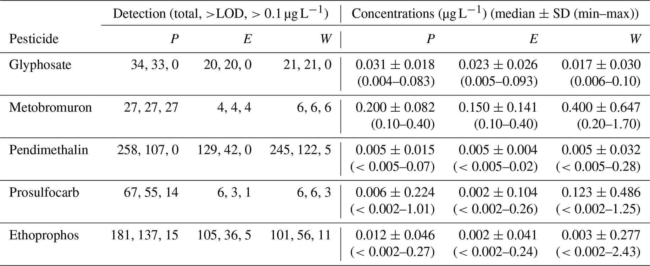
2.2 Pesticide detection, usage, and properties
Jersey Water, the sole water company and provider on the isle of Jersey, regularly tests and scans the quality of the raw water from the reservoir offtake for a wide range of different pesticides. Five active pesticide ingredients currently or recently in use in the catchment showed evidence of significant concentrations in the reservoir offtake for the drinking water supply. These included the herbicides glyphosate, metobromuron, pendimethalin, and prosulfocarb, and the nematicide and insecticide ethoprophos. During the 2016–2019 period, the sampling frequency of these pesticides was not the same (Table 1): pendimethalin and ethoprophos were sampled on approximately a weekly basis all year round, whereas prosulfocarb was generally sampled on a weekly basis from mid-February to the end of May, bi-weekly in January, and every 3 to 5 weeks during other periods. The monitoring of glyphosate and metobromuron was more sporadic and only done during spring and early summer with no sampling taking place in the autumn and the winter. Metobromuron was most frequently observed above the drinking water standard, followed by ethoprophos, prosulfocarb, and pendimethalin (Table 1). Ethoprophos was not included in the final model, as its use has now been discontinued. In consultation with Jersey Water, it was instead decided to include the nematicide fluopyram, as it was considered to be a likely replacement for ethoprophos and, hence, a potential future risk to the reservoir water quality. Monitoring data for fluopyram are not available, as it is currently not widely used in the catchment. However, fluopyram is known to be used at lower application rates than ethoprophos, making its potential risk of contaminating the water supply intrinsically lower, notwithstanding its relatively high mobility and greater persistence.
Table 1Summary of the pesticide monitoring data by location (P: Pump; E: East stream; W: West stream) in the Val de la Mare (VDLM) catchment from 2016 to 2019. Detection data are summarised as the total number of samples, the number of samples above the limit of detection (LOD), and the number of samples above the drinking water standard of 0.1 µg L−1. The concentration data are summarised as the median ± standard deviation (SD), and the range (minimum to maximum) of the observed concentrations is given in parentheses.
Data on pesticide application rates and timing for the 2016–2018 period were obtained from the Jersey Royal Company, the main potato crop grower in the area who manages ca. 50 % of the catchment area, alongside agronomic data on crop coverage and crop rotation for the 2010–2018 period. Pesticide usage (Table 2) was estimated assuming that the available agrochemical data were representative of the whole catchment. Glyphosate was mostly applied in January (mean day of application 23 January), whereas other pesticides were typically applied in February (mean day of application 11–16 February). Hence, only the months from January to March were represented in the model in order to allow for a potential 1-month delay in pesticide application. The usage of pesticides on other crops in the catchment was limited to the utilisation of glyphosate for spraying off grass prior to cultivation and the utilisation of pendimethalin on barley.
Table 2Summary of pesticide properties considered in the model (Lewis et al., 2016) and mean application rates in the study catchment. The abbreviations and parameters used in the table are as follows: AI – active ingredient, Koc – pesticide adsorption coefficient on soil organic carbon, and DT50 – time for 50 % of pesticide to be degraded in soil. The values shown are mean values, and the ranges are given in parentheses.
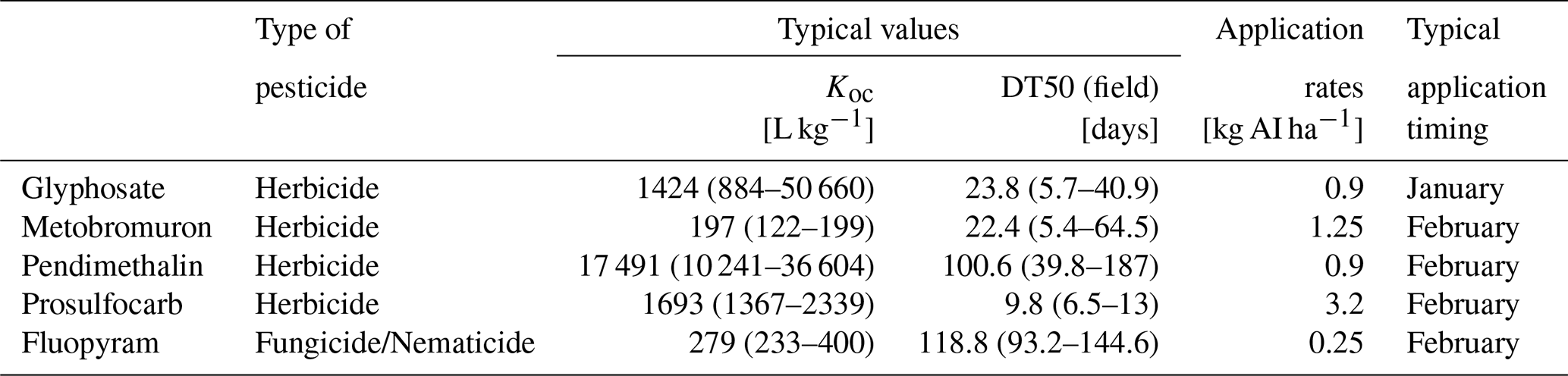
Key pesticide properties for assessing the risk to water quality were extracted from a publicly available database (Table 2; Lewis et al., 2016). These included the Koc coefficient, which represents the adsorption of the pesticide onto the organic carbon of soil, subsoil, and vadose zone materials, and the half-life (DT50), which represents the degradation rates during transport through each of these layers (Table 2). A third process – that of volatilisation – was not considered, as this is relatively minor in most cases, and the omission of this process will provide a conservative estimate for the impact on groundwater. The retention of pesticides by the soil and subsoil materials to which it is applied depends on adsorption to organic and mineral surfaces. Soil sorption processes are complex and have been the subject of substantial research in the past. Pesticide sorption is influenced by both the chemical characteristics of the pesticide and soil-specific properties, such as the soil organic carbon (SOC) concentration, clay content, pH, and soil moisture content. For neutral non-polar pesticides, it is well documented that pesticide retention is strongly correlated with the SOC concentration, with other factors such as clay content, pH, and aeration status playing a subsidiary role (Kah and Brown, 2006; Wauchope et al., 2002). For weakly ionisable pesticides with ionic equilibrium constants near the range of soil pH, sorption may be highly sensitive to the pH of the sorbing soil. However, none of the pesticides considered for the modelling here are considered weakly ionisable; therefore, only the role of SOC content on pesticide retention was considered in the model by including the pesticide adsorption coefficient Koc. The degradation rate of pesticides in soil and subsoil depends principally on the microbiologically mediated decomposition and, as such, is also strongly influenced by SOC (Jury et al., 1987; Kah and Brown, 2006). Some chemical degradation of pesticides on mineral surfaces can also occur, which may be more important for the subsoil and vadose zone, but biological degradation is seen as the main pathway in most cases (Fomsgaard, 1995). In most instances, the time for 50 % disappearance (DT50) or 90 % disappearance (DT90) is determined.
2.3 Catchment characteristics
Monthly rainfall and temperature data were available from a single meteorological station in the study catchment, operated by Jersey Water for the period from 2014 to 2019. Due to the short duration of this record, additional monthly total rainfall and mean monthly temperature data (from 1894–2019) were obtained from the government of Jersey website (https://opendata.gov.je/organization/weather, last access: 24 February 2022). Data for the years 1981–2019 were then used in combination with the catchment-based meteorological data to calculate monthly mean and standard deviation as priors for the model. Mean monthly potential evapotranspiration (PET) and actual evapotranspiration (AET) were calculated using the approach in Pistocchi et al. (2006); for more information, the reader is referred to Appendix A.
Spatial environmental data were processed and collated in a single GIS shapefile. Visualisation, geographical analysis, and processing of spatial data sets were done in QGIS 3.12.2 (QGIS.org, 2022, QGIS Geographic Information System, QGIS Association), while ArcGIS 10.1 (ESRI, 2011) was used for the generation of the digital terrain model (DTM). The following data sets were used to inform model parameterisation.
Land parcels that fell within the VDLM catchment area were selected and filtered using feature types (i.e. cultivation) to identify cultivated fields. The field selection was supplemented by visual inspection using satellite imagery provided by Google in order to ensure that only cultivated fields were selected. This resulted in the selection of 200 fields, which were assigned a dominant crop type for the 2010–2018 period by spatially joining field polygons with layers containing crop type information. Crop operation information available for 56 fields within the catchment was used to determine the timing and pesticide application rates (Table 2) and to inform the prior distributions in the model.
A 1 m resolution hydrologically corrected DTM of the VDLM catchment area was created using digital line contours at a 1 m interval provided by Jersey Water and the “Topo to Raster” tool in ArcGIS; the DTM was used to calculate mean elevation and slope (in degrees) for each field polygon within the VDLM catchment. Topographic connectivity was derived by calculating the horizontal distance from the polygon vertex nearest to the stream features using the “Distance to Nearest Hub” tool in QGIS. Because the study catchment is flat with relatively uniform slopes, we opted here to base the topographic connectivity on the simple “distance to stream” approach. This approach has previously been shown to be accurate for assessing connectivity (e.g. Grauso et al., 2018). For other catchments, it might be more appropriate to use a connectivity based on actual flow direction.
The overall depth of the soil column is a key characteristic of the soil that influences the attenuation of pesticides applied to the surface. Depth to groundwater was calculated for each field using a 5 m groundwater level contour map of Jersey prepared by the British Geological Survey and provided by Jersey Water (Tim du Feu, personal communication, 20 May 2020) by importing and georeferencing the map in QGIS, digitising the contour lines, and combining them with field polygons.
Soil water retention, conductivity, natural drainage, and anthropogenic characteristics, such as plough pans, were also considered in model parameterisation. There has been no systematic survey of the soils of Jersey in the traditional sense of classifying and grouping soils according to their pedology. Brief descriptions of “soil series” were given in Jones et al. (1990), and the Soil Atlas of Europe (European Soil Bureau Network, 2005) shows a single soil type, Dystric Cambisols, for the whole island of Jersey at a 1:2 500 000 scale. Due to this lack of detailed soil mapping, the Hydrogeological map of Jersey (Robins et al., 1991) was used to identify soil hydrological units based on the three hydrogeological formations identified in the VDLM catchment (Fig. 1b). These three soil hydrological units consisted of soils developed on loess, aeolian (blown) sand, and shales respectively. Both loess and sand are periglacial Quaternary deposits that are relatively common throughout northern Europe. Soil hydrological data for similar soils are contained within the HYPRES (HYdraulic PRoperties of European Soils) soil hydrological database (Wosten et al., 1999, 1998); hence, this database was used to derive the soil hydrological properties necessary for the modelling of pesticide attenuation.
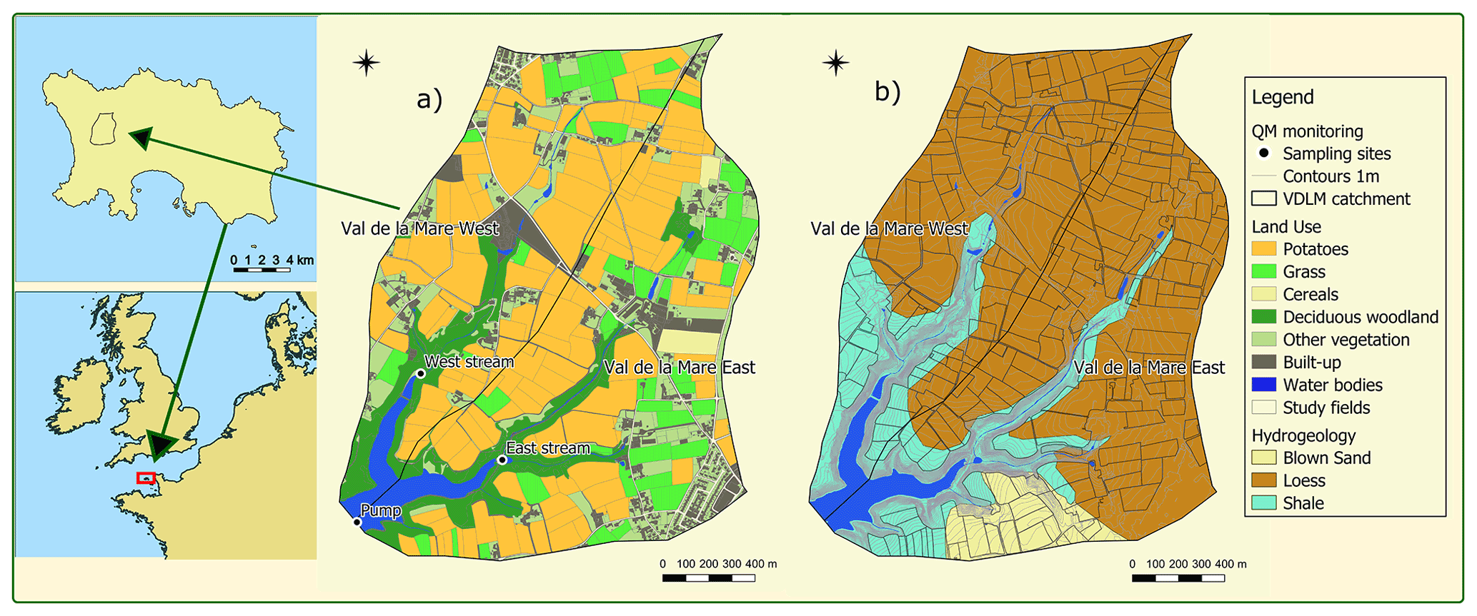
Figure 1Location of the Val de la Mare (VDLM) study catchment on the island of Jersey. Panel (a) shows the three water quality monitoring sites (Pump, West stream, and East stream) and the land use in the catchment, and panel (b) shows the hydrogeology. Country boundaries were taken from https://www.gadm.org/ (last access: 24 February 2022), and hydrogeological data were digitised from the Hydrogeological map of Jersey available under the Open Government Licence v3.0 (contains © British Geological Survey materials, UKRI, 1992)
According to the descriptions of soil series in Jones et al. (1990), the soils developed on these three hydrogeological units are generally well to moderately well drained with no real inhibition to the downward movement of water. Soil hydrological properties derived from the HYPRES database supported this assumption, with mean saturated hydraulic conductivity largely greater than 10 cm d−1. Less than this would indicate the presence of a slowly permeable horizon (MAFF, 1988) with some degree of ponding within the soil.
Local knowledge suggested that some of the soils in the catchment could have a plough pan potentially as deep as 60 cm below the surface. This layer is likely to restrict the downward flow of water through the soil and increase the likelihood of near-surface runoff and was included as one of the soil parameters that could be manipulated within the model. In the absence of data in the HYPRES database on plough pans, a value of 0.02 cm d−1 was selected as a worst-case estimate of plough pan hydraulic conductivity based on Koszinski et al. (1995), who reported hydraulic conductivity of compacted soil of between 0.02 and 3 cm d−1.
Laboratory measurements of topsoil soil organic matter (SOM) content and pH were available for 40 and 37 fields within the VDLM catchment respectively, most of which were cultivated with Jersey Royal potatoes (32). The SOM content ranged from 1.9 % to 3.8 % with a mean of 2.5 %: the mean SOM for loess was 2.5 % (1.9 %–3.8 %), and the mean for shale was 2.3 % (1.9 %–3.4 %). The median SOM was slightly greater for the six fields found on grassland (3 %) than for the potato fields (2.3 %). Soil pH ranged from 5.3 to 7.2 with a mean pH value of 6.4, and the mean soil pH was slightly greater for the potato fields (6.4) than for grassland (6.1). However, as this information was not available for all fields and only for the topsoil, these data were not used in the model parameterisation. Instead, model sensitivity to using observed SOM concentrations vs. those derived from the HYPRES database was examined and was found to be negligible; therefore, the converted HYPRES SOC values (by dividing SOM by 1.724) were used as priors in the model to ensure spatial consistency.
2.4 Field attributes
The spatial data described in Sect. 2.3 were used to inform the parameterisation of the model variables. It was found that most study fields within the VDLM catchment lay on relatively flat ground (with 152 fields having a mean slope of less than 3∘), and the elevation range was also relatively small (from 67 to 99 m). Loess was the dominant soil parent material in 155 fields, while soils derived from Jersey shale or blown sand were dominant in the remaining 31 and 14 fields respectively. Loess covered the central and northern part of the VDLM catchment, shale was found in the south-western part of the catchment, and blown sand was found in the south-eastern part of the catchment. Most study fields had a sandy silt loam (120) or sandy loam (59) soil texture class. Fields with a sandy silt loam texture were mostly underlain by the Loess formation (101), whereas fields with sandy loam texture were mostly underlain by the Jersey Shale Formation (36) and blown sand (12).
The horizontal distance of VDLM fields to the stream network was used to represent field connectivity to the stream network and the reservoir. The median horizontal distance was 119 m, with 91 fields located within 100 m of the stream network. The depth to groundwater within the VDLM catchment ranged from 0 to 20 m, but most of the catchment area (56 %) had a shallow aquifer less than 5 m deep (117 fields), with a further 54 fields having groundwater depths of between 5 and 10 m.
2.5 Spatial Bayesian belief network risk model
We have developed a probabilistic model, based on spatial Bayesian belief networks (BBNs) (Appendix A) in order to evaluate the spatial and temporal variability of the intrinsic pesticide pollution risk from critical source areas within the VDLM study catchment. The model aims to provide a field-level assessment of the relative water pollution risk characteristics of each field, made available as probabilistic map layers. The developed approach integrates the various information sources described above and includes causal relationships between both discrete and continuous variables in a hybrid BBN. The general principles and theory of Bayesian networks have been described extensively elsewhere (Korb and Nicholson, 2010; Moe et al., 2021) and will not be discussed in detail here.
The model structure and development were informed by expert knowledge and stakeholder feedback. Hydrologically, the VDLM reservoir was assumed to be fed by the West and East streams (Fig. 1) as well as by groundwater, and the groundwater aquifer was assumed to be unconfined and homogenous. Thus, pesticides applied to a given field could either leach to groundwater or could be transported directly to the reservoir or one of the streams through surface runoff. Therefore, the risk assessment model accounted for pesticide losses via both groundwater leaching and overland flow, with the final assessment based on the combination of both. Both transport pathways are influenced by three key factors, namely soil and site characteristics, climate and hydrology, and land management (e.g. pesticide usage and properties, and land use) (Fig. 3, Appendix A).
In the following, the modelling of the groundwater leaching and the overland flow risk components is described. In both cases, we are interested in determining how much of the applied pesticide mass L0 [kg ha−1] may eventually reach either groundwater via leaching (Lgw [kg ha−1]) or surface water via overland flow (Lof [kg ha−1]) from a given field. To ensure mass balance, we assumed that only a proportion fleach of the applied pesticide mass would be available to leaching for each field, while the remaining proportion would run off to surface water. During transport to groundwater and surface water, the pesticide can undergo attenuation with the degree of attenuation determined by the respective groundwater and surface water attenuation factors AFgw (Eq. 10) and AFof (Eq. 11) (as described in the following sections). Thus, the respective pesticide loads that reach groundwater via leaching and surface water via runoff from a given field were given by
Conceptually, this way of calculating the pollution risk to groundwater and surface water is similar to the pesticide impact rating index proposed by Kookana et al. (2005) and to the InVEST nutrient delivery model (Sharp et al., 2020). For the modelling here, it was assumed that the fraction of the applied pesticide to land that would be available to leaching fleach equalled the ratio of infiltration to excess rainfall.
The combined pesticide load from a given field was the sum of the leaching and the overland flow component.
This combined pesticide load was converted to a surface water concentration Csw [µg L−1] to evaluate the risk to surface water as follows:
where Ac is the total area of all fields in the catchment (192 ha), and Vres is the water volume in the reservoir (938 700 m3). Equation (3) is a very simplified way of evaluating the field-level risk; it is essentially assumed that the combined load from the field in question represents the average load from all fields in the catchment. This allows the combined pesticide load from the given field to be converted to a concentration in the reservoir, which can then be compared to the regulatory standards based on which the risk can subsequently be assessed. Hence, if the combined pesticide load from a field resulted in Csw exceeding the standard of 0.1 µg L−1, this field was considered high risk (see Appendix A).
2.5.1 Groundwater leaching risk assessment
The conceptual model for the pesticide leaching to groundwater applied in this study catchment (Fig. 3) followed on from the screening model proposed by Jury et al. (1987). The model assumes that a single pesticide mass flux is applied to the soil surface (z=0). The pesticide is assumed to dissolve in the infiltrating rainwater and move downward through the soil profile by leaching at a constant water infiltration rate Jw [m d−1], which is here determined by the amount of excess rainfall and the physical properties of the soil (Appendix A). The pesticide is assumed to move downward through the soil by piston flow (i.e. no dispersion) while undergoing linear adsorption and first-order decay. Given these assumptions, the pesticide transport and fate can be described by the following mass balance equation (Jury et al. 1987):
where C [µg L−1] is the pesticide concentration in solution (the water phase), θw is the volumetric water of the soil, µ [d−1] is the first-order degradation constant, and RF is the retardation factor given by Jury et al. (1987) as
Here, Koc [L kg−1] is the organic carbon partition coefficient, and ρb [kg L−1] and foc [kg kg−1] are the soil bulk density and the organic carbon content of the soil respectively. The retardation factor describes the velocity of the solute pesticide relative to the infiltrating water. The solution to the mass balance equation (Eq. 4) for an instantaneous mass injection m0 [kg ha−1] can be written as
Here, m(z) [kg ha−1] is the pesticide mass contained within the pulse when it reaches depth z [m], and AF is the attenuation factor given by Stenemo et al. (2007):
where DT50 [d] is the half-life of the pesticide. AF expresses the fraction of the applied pesticide that will reach depth z and can take values between zero (none of the applied pesticide will reach depth z) and one (all of the applied pesticide will reach depth z).
It is well known that the organic matter concentration and microbial population density decrease with depth in the soil profile; hence, both the pesticide retardation and decay rates are expected to decrease with depth (Jury et al., 1987; Kookana et al., 2005). To account for this effect, the model divided the soil profile into three regions (Fig. 2): (a) the A horizon (topsoil), which was assumed to be 30 cm thick and to be the most microbially active region; (b) the B horizon (subsoil), which was also assumed to be 30 cm thick; and (c) the vadose zone, which extends from the bottom of the B horizon to the groundwater table and was assumed be the least microbially active region. Furthermore, in the VDLM catchment, the presence of low-permeability soil pans was believed to be widespread due to intensive management. When such a soil pan was present, it was assumed to be 10 cm thick and to be situated within the B horizon (Fig. 2). Each of the regions was characterised by uniform values of the volumetric water content, soil bulk density, organic carbon content, and decay rates (Appendix A).

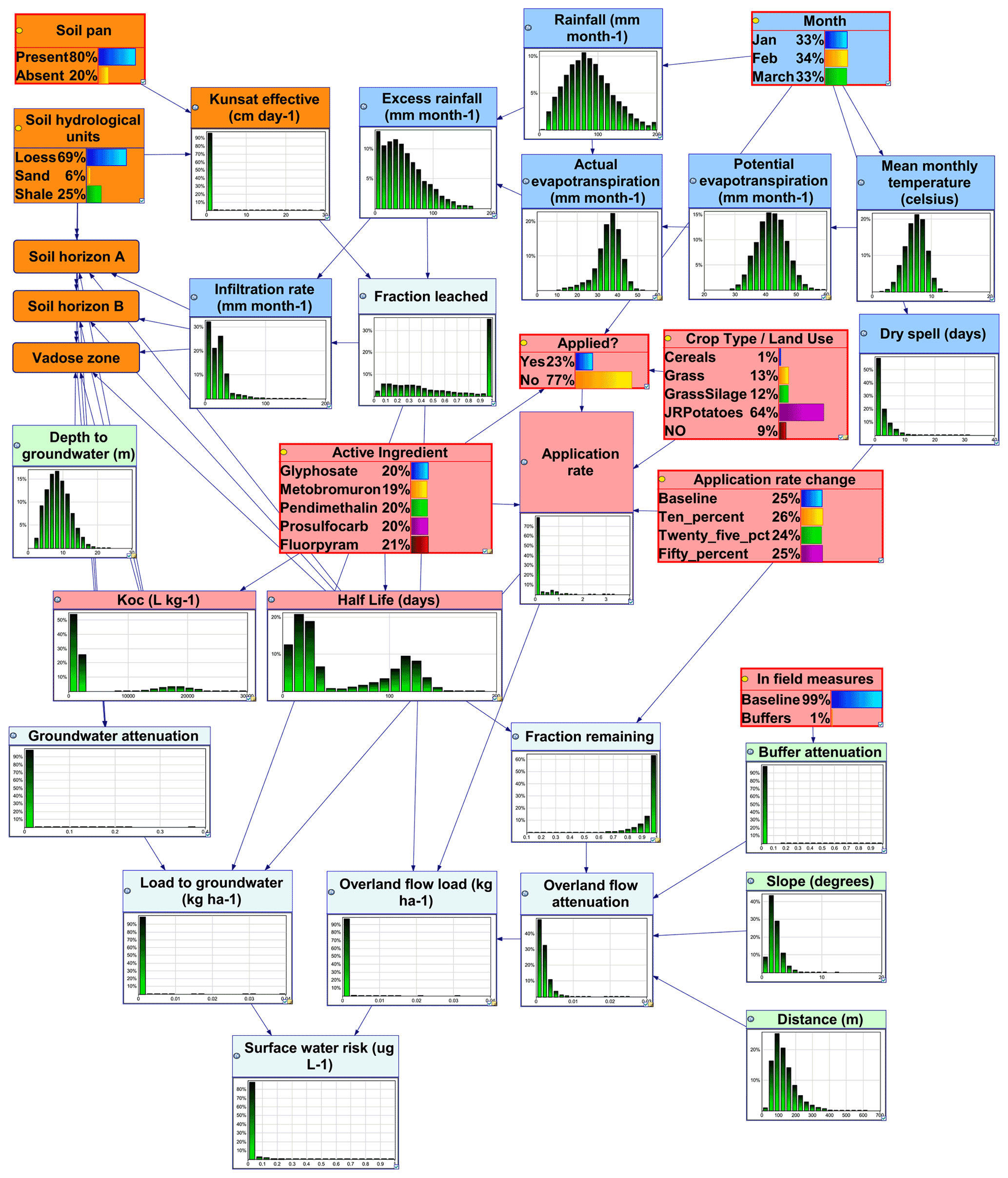
Figure 3Conceptual structure of the pesticide risk model. Blue: climate/hydrological variables; orange: soil variables; pale green: site-specific variables; red: land-management-/pesticide-specific variables. Nodes with a thick red border show discrete variables that can be manipulated to model management scenarios. Histograms show continuous variables included in the model.
An attenuation factor can be calculated for each of the three zones AFi, where the subscript i refers to the A horizon (A), B horizon (B), or vadose zone (VZ).
where RFi and DT50i are the respective retardation factor and half-life in zone i, and [d] is the average time it takes the infiltrating water to travel through a given zone i:
Here, and di [m] are the effective volumetric water content and the thickness of horizon i respectively.
The aim of the leaching risk model is to predict the pesticide load reaching the groundwater Lgw (Eq. 1). To do this, an effective attenuation factor AFgw is calculated by multiplying the AF for each of the three soil profile regions:
Overall, the pesticide leaching risk assessment reflected a set of soil-specific factors (organic carbon concentration, bulk density, water content, and thickness for each of the three layers), pesticide-/management-specific factors (application rate, Koc, and half-life), and climatic factors (rainfall and temperature from which groundwater recharge and runoff rates were estimated).
2.5.2 Overland flow risk assessment
The transport of pesticide from the site of application to surface water via overland flow is complex. Pesticides can leave a field either dissolved in runoff water or attached to eroded soil colloids. Because the amount of eroded soil lost from a field is usually small compared with the runoff volume, losses via runoff are generally considered more important than losses via erosion for most pesticides. Only for strongly adsorbing pesticides, the erosion pathway becomes the more dominant avenue for loss (Reichenberger et al., 2007). However, in the present study, potato cropping was the dominant land use, which has been shown to be highly erosive (Vinten et al., 2014); therefore, the runoff and erosion transport pathways have been lumped into one for the modelling of the overland flow losses. Other processes such as spray drift and volatilisation may also transport pesticides directly to surface water, but these were considered less important relative to the other pathways and were, therefore, not included in the modelling.
The overland flow pesticide load Lof [kg ha−1] was calculated using Eq. (2) and assuming that the fraction of applied pesticide that will run off a given field and reach the reservoir (AFof) can be estimated as
where tro [d] is the time passing between pesticide application and the occurrence of a runoff event, and fslope, fdist and fbuffer are the slope, distance, and buffer correction factors respectively.
Here, S [∘] is the local slope, dfr [m] is the distance from the field to the reservoir, and E [%] is a retention efficiency of a field buffer strip. The above approach for modelling overland flow attenuation follows on from REXTOX (OECD, 2000). In REXTOX, the time between pesticide application and the occurrence of a runoff event is assumed to be 3 d, whereas we assumed the time to depend on the month of application (see Appendix A). For simplicity and because we considered the contribution from both runoff and erosion, the available amount of pesticide available for runoff was not corrected for sorption or for plant interception. The slope correction was assumed to be a linear function up until a local slope of 10∘, beyond which no correction took place; a similar slope cut-off value is assumed in REXTOX and in studies such as Drewry et al. (2011). The buffer correction factor was informed based on a review of buffer retention efficiencies (Reichenberger et al., 2007). It should be noted that REXTOX only considers pesticide losses via runoff from fields immediately adjacent to surface waters and, therefore, does not include a distance correction factor. Here, we assumed that the attenuation was inversely proportional to the distance from the reservoir. The distance correction and cut-off value were based on the assumption that no significant pesticide attenuation would occur within 1 m of a watercourse. This assumption was informed by Reichenberger et al. (2007), who state that “… even if pesticide-loaded runoff infiltrates into a riparian buffer strip, the groundwater table below the strip will be rather shallow (unless the stream bed is deeply cut into the floodplain), and the groundwater feeds into the nearby stream … we conclude that riparian buffer strips are most probably much less effective than edge-of-field buffer strips.”.
The above presented approach enabled us to (a) assess relative pesticide loss risk from all fields in the study catchment, (b) compare overland flow risk to groundwater leaching risk for all fields, and (c) evaluate optimal spatial targeting and the effect of available mitigation measures in the whole study catchment.
2.6 Model implementation and testing
The hybrid BBN model was constructed in GeNIe 3.0 (https://www.bayesfusion.com/, last access: 24 February 2022). Prior probabilities for network variables were calculated from data described in Sect. 2.2 and Appendix A. Discrete variables were assigned a number of mutually exclusive “states” with conditional probabilities captured in conditional probability tables (CPTs). Prior probability distributions for continuous nodes were fitted to available data using the minimum (min), maximum (max), 5th, 50th, and 95th percentiles of the cumulative probability distribution (O'Hagan, 2012) in the SHELF package (Oakley, 2020) in the open-source statistical modelling software R (The R Project for Statistical Computing 4.0.1; R Core Team, 2019). In the SHELF package, several statistical distributions were fitted to these statistical moments, and the distribution with the closest fit to the original percentiles was selected as a prior for modelling. In a few instances, where the best fitting distribution available in SHELF was not supported in GeNIe, the next best fitting available distribution was selected. For Koc and the half-life, where we had limited information to inform the prior distribution, we assumed that these variables belonged to a truncated normal distribution (truncated at zero), and we considered the mean to closely represent the median (i.e. the 50th percentile). Further, we assumed that the min closely approximated the 1st percentile and that the max closely approximated the 99th percentile, and we have used them as such. We rounded min and max up or down to the nearest decimal point to make them just a fraction smaller or larger than the 1st and 99th percentiles in the model fitting.
A discretised version of the model was then exported to R and applied at the field level, using the bnspatial package (Masante, 2017). A discretisation method selected for each node is described in Appendix A. Discretisation was based on a mix of expert opinion (e.g. soil organic carbon and hydraulic conductivity, as well as groundwater pesticide load and the final surface water risk, which were discretised considering the likelihood of exceeding the drinking water standard concentration of 0.1 µg L−1), accepted values from the literature (e.g. pesticide Koc and half-life), uniform cases (e.g. rainfall, temperature, and PET), and uniform interval width (e.g. depth to groundwater, distance, and slope). Child nodes such as AET, infiltration rate, and overland flow attenuation were discretised using interpolation to ensure that conditional probabilities for the combination of parent node states (low/low, medium/medium, and high/high) were meaningful. Application rate discretisation was based on equal counts but was adjusted to ensure that change in application rates would result in a shift between risk classes, with the number of states maximised to allow sensitivity to change while considering model runtime. This was done empirically by progressively increasing the number of discretisation intervals and adjusting discretisation boundaries whilst checking that probabilities of pesticide application rates conditional on the application change rate resulted in a probability density shift by one state.
Available spatial GIS layers were used as “hard” evidence to set states for relevant nodes in the discretised model and produce spatially explicit simulations of probabilistic outcomes. Essentially, the discretised model was applied field by field using field-specific inputs from the GIS layers as hard evidence.
Uncertainty in the simulated outcomes in the spatial implementation of the model was evaluated by calculating the Shannon entropy index of the target nodes. The entropy H(X) for node X is defined as
The entropy quantifies the information content within a node; it equals zero if X is known with certainty and is maximised when X is unknown (i.e. X is given by a uniform distribution).
Sensitivity analysis of the discretised model was undertaken in GeNIe using the algorithm of Kjærulff and van der Gaag (2000) that calculates a complete set of derivatives of the posterior probability distributions over the target nodes for each of the numerical parameters of the Bayesian network, using the two modelled risk pathways and the combined risk as target nodes. The Euclidean distance measure, which quantifies the distance between the various conditional probability distributions over the child node, conditional on the states of the parent node, was used to calculate the strength of the influence between variables (Koiter, 2006).
For model validation, simulated values of surface water risk (i.e. surface water pesticide concentration in micrograms per litre) in the hybrid model were compared to the limited available water quality observations for four active ingredients from January to March (see Sect. 3.4). This was done by generating 10 000 random simulations for each pesticide in the hybrid BBN using forward stochastic simulation, with the random samples being drawn from the nodes' prior probability distributions. It was found that 10 000 simulations were adequate to achieve stable model convergence. Note that the prior probability distributions for the different nodes in the hybrid model reflect the catchment as a whole (e.g. the prior probability distribution for the crop type node reflects the actual distribution of crop types in the catchment). This means that, although spatial patterns and potential spatial correlation between inputs are not accounted for explicitly in the hybrid model (unlike for the spatial application of the model using bnspatial, where the model is applied on a field-by-field basis), the simulated surface water concentrations in the hybrid model can be considered representative of average catchment conditions. Model credibility was further evaluated using stakeholder feedback.
2.7 Simulated scenarios
A questionnaire was used to elicit stakeholder feedback regarding potential alterations to the management of crops/pesticides and mitigation strategies from steering group members representing a grower, a regulator, and a drinking water supplier in the study catchment to develop plausible pesticide mitigation scenarios. The agreed scenarios included the following:
-
baseline risk for five active ingredients;
-
delayed pesticide application by 1 month (January–February and February–March);
-
reduction in the pesticide application rate by 10 %, 25 %, or 50 %;
-
additional buffering of fields to reduce overland pesticide runoff;
-
presence/absence of a soil pan;
-
maximum intervention (combination of 50 % reduction in the pesticide application rate, management of the plough pan, delayed application timing, and field buffer installation).
A number of detailed mechanistic models have successfully simulated pesticide dynamics at the plot and catchment scale (Köhne et al., 2009; Villamizar et al., 2020). However, detailed observational data required for the calibration and validation of complex models are not widely available to managers in many drinking water catchments. In this case study, in addition to sparse water quality observations, process-based modelling was hindered by the complex water transfers and limited gauging at the reservoir outlet, which prevented the calculation of the hydrological balance due to a lack of data on water transfers from neighbouring catchments and the productivity of the desalination plant. Difficulty with closing the water balance without considerable uncertainty is a known problem in many catchments that affects the practical application of many modelling approaches (Beven et al., 2019). Therefore, to support decision-making, we developed a probabilistic model of intrinsic vulnerability to pesticide pollution within a Bayesian framework to allow the assessment of intrinsic pesticide risk and to inform management. As pesticide risk assessment is inherently uncertain, due to many complex and poorly characterised processes, the graphical BBN model helps to improve the transparency of the risk management process (Carriger and Newman, 2012). Furthermore, the probabilistic assessment provided by the BBN methodology is more in line with the classical definitions of risk than the more commonly used single-value risk quotients (Moe et al., 2021). The model represents key processes to capture combined uncertainties stemming both from observational data and limited knowledge (Sahlin et al., 2021).
3.1 Can we characterise the spatial and temporal variability of pesticide pollution risk from groundwater leaching and overland flow in a data-sparse catchment?
The causal structure of the hybrid BBN model designed in GeNIe is shown in Fig. 3. The network consists of 45 nodes and 75 arcsec. The results of the spatial simulation of the groundwater leaching pesticide flux, the overland flow pesticide flux, and the overall surface water risk are shown in Figs. 4–6. The spatial application of the discretised model for five active ingredients has mostly shown a uniform low degree of pesticide leaching to groundwater across the 3.1 km2 study catchment, with the exception of prosulfocarb applied at the highest application rate (Fig. 4). The largely low groundwater leaching risk is not surprising due to the very high groundwater attenuation rates, which result from the considered pesticides being neither particularly mobile (all have relatively high Koc values) nor persistent (all have relatively short half-lives) (Table 2). Piffady et al. (2020) also found that subsurface vulnerability was the least discriminating spatial layer, as compared to other hydrological pathways.
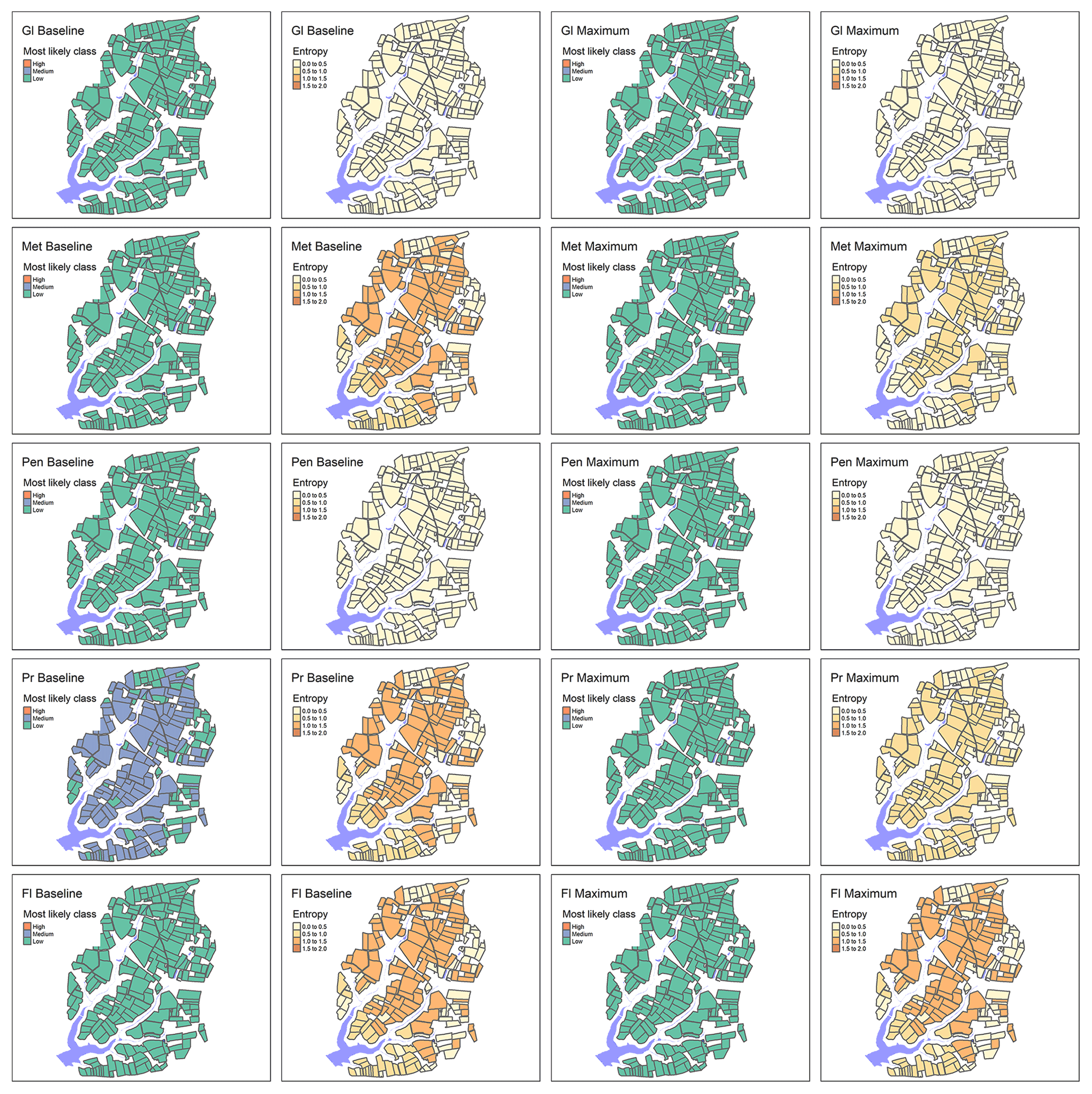
Figure 4Spatial variability and associated uncertainty (entropy) in the groundwater leaching risk under current practices for the five active ingredients under baseline and maximum mitigation scenarios: Gl – glyphosate, Met – metobromuron, Pen – pendimethalin, Pr – prosulfocarb, and Fl – fluopyram.
Conversely, the overland flow pesticide loads showed a distinct spatial variability, with most risky fields located on the steepest slopes closest to surface water bodies (Fig. 5). Figure 5 also suggests that more of the risky fields are located around the West stream, which agrees with the fact that the observed pesticide concentration levels in the West stream are generally greater than in the East stream (see Table 1). This can be explained by more fields being treated with pesticides in the western part of the catchment (i.e. more fields where the dominant land use is potato) but also by more permeable hydrogeological formations (i.e. blown sand) and soils being located in the south-eastern part of the catchment; hence, less runoff is expected to be generated in the latter area (Fig. 1b). As the overland pesticide load is more closely related to the final surface water risk than is the groundwater pesticide load (Fig. 7, Table 3), the resulting risk maps for overland load and surface water risk load look similar (Figs. 5, 6).
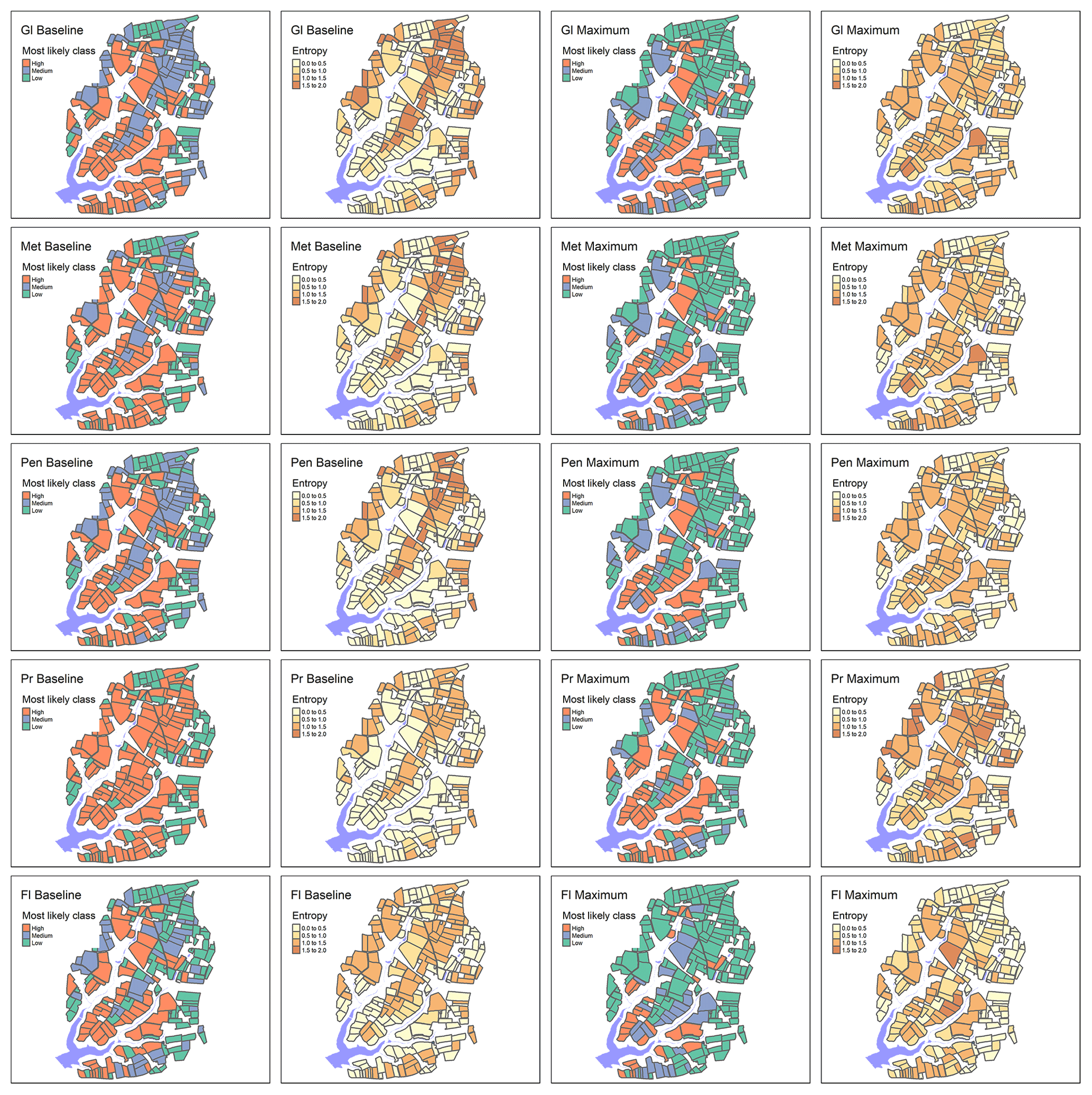
Figure 5Spatial variability and associated uncertainty (entropy) in the overland runoff pesticide loads under current practices for the five active ingredients under baseline and maximum mitigation scenarios: Gl – glyphosate, Met – metobromuron, Pen – pendimethalin, Pr – prosulfocarb, and Fl – fluopyram.

Figure 6Spatial variability and associated uncertainty (entropy) in the surface water risk under current practices for the five active ingredients under baseline and maximum mitigation scenarios: Gl – glyphosate, Met – metobromuron, Pen – pendimethalin, Pr – prosulfocarb, and Fl – fluopyram.
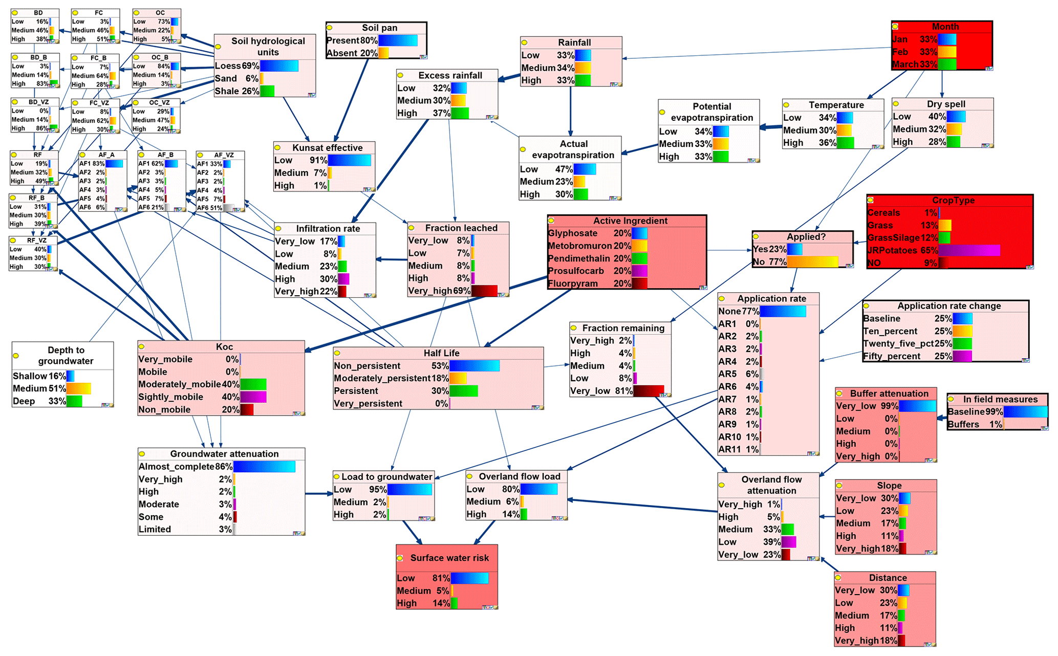
Figure 7Strength of influence and sensitivity analysis implemented in the discrete version of the network (Kjærulff and van der Gaag, 2000) using surface water risk, groundwater load, and overland flow load as target nodes. Deeper red colouring shows the more influential variables. The thickness of the arrows indicates the strength of the influence between two directly connected nodes calculated as the Euclidean distance.
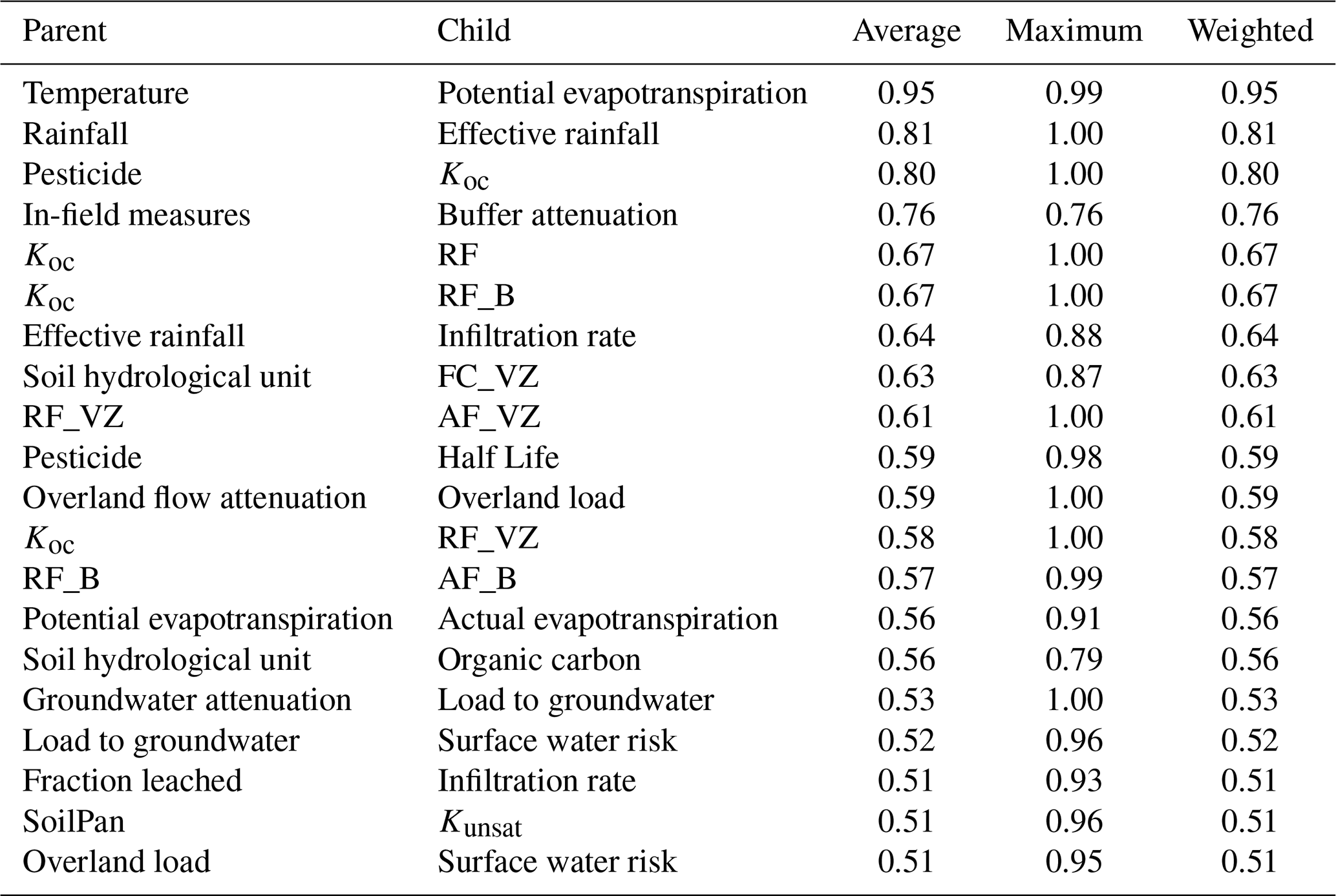
Table 3Strength of influence for the top 20 most closely related variables (Euclidean distance >0.5). The abbreviations used in the table are as follows: RF – retardation factor, AF – attenuation factor, VZ – vadose zone, and B – soil horizon B.
The entropy calculation for overland flow pesticide loads (Fig. 5) and surface water risk (Fig. 6) suggests that the risk assessment status class is more certain for the fields closest to the streams in the baseline scenario, whereas the uncertainty is more evenly distributed across the catchment for the maximum intervention scenario. The assessment of groundwater leaching pesticide loads is generally more certain (Fig. 4). Regardless of the absolute values, the relative difference in entropy between different management scenarios and risk status classes is informative for advising management interventions and safeguarding managers from putting too much or too little confidence in the final risk assessment (Sahlin et al., 2021).
The application of continuous and hybrid networks in environmental risk assessment is rare (Kaikkonen et al., 2020). The integration of BBNs with GIS for spatial risk assessment has recently been increasing, but it is still limited (Carriger et al., 2021; Guo et al., 2020; Kaikkonen et al., 2020; Pagano et al., 2018). A major advantage of the BBN approach presented here over existing index methods for pesticide risk assessment is that the risk and the associated uncertainty can be determined and mapped, thereby allowing the confidence in the results to be directly assessed. The hybrid network allows more detailed characterisation of multiple processes and their uncertainty than a typical index-based GIS method. However, the need to discretise the network for spatial applications currently presents a major methodological limitation, leading to loss of information, and would merit further research and development.
3.2 Which factors are most influential on the intrinsic pesticide pollution risk?
Sensitivity analysis has identified the most influential parameters affecting the pesticide leaching and the overland flow pesticide loads. Figure 7 shows the result of sensitivity analysis graphically, with nodes coloured in red being more important for the calculation of the posterior probability of the pesticide risk nodes. Pesticide pollution risk was particularly sensitive to crop type, time of application, overland attenuation, slope, and proximity to the surface water body. Crop type directly determines the expected amount of pesticide applied in a given field, whereas the time of application affects expected rainfall and length of a dry spell following application. Alongside the soil hydraulic conductivity, the latter two influential variables determine the amount of infiltration and overland flow. It is apparent that not all variables in the model contributed strongly to the final risk assessment; hence, model simplification may be possible. However, it may be advisable to test model transferability to other locations first to confirm these relationships before omitting potentially uninfluential variables. For example, depth to groundwater appears to be uninfluential in this study catchment, which may be explained either by the relatively uniform shallow depths and uncertain hydrogeological data or by most pesticide retention and degradation taking place in the A and B soil horizons, with limited influence from the vadose zone. These hypotheses could be tested in a study catchment with a better understanding of the subsurface. Evapotranspiration calculations also appear to have limited impact and could potentially be omitted from the model for simplification. While the above influential variables have been previously identified among important factors for rapid overland flow risk (Bereswill et al., 2014; Tang et al., 2012), our modelling approach allows one to distinguish between generic risk factors and variables with the greatest influence on pesticide pollution risk in a local catchment setting. Coupled with the ability to identify critical source areas as well as how they change at a monthly time step, our approach offers a major advancement compared with static GIS-based risk index assessment approaches (e.g. Quaglia et al., 2019).
Figure 7 shows the results of the strength of influence analysis, where the thickness of the arrows represents the strength of influence between two directly connected nodes based on the Euclidean distance between the probability distributions. The top 20 most closely related variables with a Euclidean distance >0.5 are presented in Table 3. All of the relationships are intuitive and build confidence in the reliable specification of the conditional probabilities and, hence, in the model simulations.
3.3 What is the effectiveness of available management interventions with respect to pesticide risk reduction?
The BBN model was applied to evaluate the effectiveness of the following mitigation measures on reducing the pesticide risks: delayed timing of pesticide application; a 10 %, 25 %, or 50 % reduction in the pesticide application rate; additional field buffers; and the presence/absence of a soil pan. Figures 8–9 show the results of the simulated management scenarios on the overland flow pesticide load of metobromuron and the groundwater leaching pesticide load of prosulfocarb respectively (similar results for the other pesticides can be found in Appendix B).
The time between pesticide application and the first runoff event is often considered critical for the mobilisation and loss of pesticide via runoff; hence, avoiding application in months with a higher probability of runoff events can potentially lead to a reduction in risk (Reichenberger et al., 2007). The figures suggest that delaying the application of pesticide until March results in a decrease in runoff risk for metobromuron but has limited impact on the leaching of prosulfocarb to groundwater, as groundwater risk is not related to the length of a dry spell and associated pesticide degradation following pesticide application.
Reduction in application rates unsurprisingly results in a reduced risk, particularly in the groundwater leaching risk (Fig. 9), which is reduced to low even after a 10 % reduction. This is in line with the findings of Reichengerger et al. (2007), who concluded that application rate reduction was one of a few mitigation measures that could address pesticide leaching to groundwater with some confidence. However, while reduction in application rates is an easy measure to implement and may lead to cost savings, it can only be implemented to the point where it remains effective, thereby potentially limiting its acceptability as a mitigation measure to farmers (Bereswill et al., 2014). The introduction of buffers reduces the runoff risk to a similar extent as a 50 % reduction in pesticide application rates for overland flow risk. Buffers, particularly edge-of-field buffers, have been found to be effective mitigation measures for the overland flow pathway (Bereswill et al., 2014; Reichenberger et al., 2007). Although buffer effectiveness is variable, most studies report efficiencies over 60 % (Bereswill et al., 2014). In addition, permanent buffers are seen as an acceptable mitigation intervention as long as farmers can be compensated for potential losses of growing area (Bereswill et al., 2014). Managing and removing potential plough pans increases the amount of infiltration into soils, thereby reducing the pesticide runoff risk to an extent that is comparable to a 10 % reduction in application rates (Fig. 8). By combining all available maximum interventions (a 50 % reduction in the pesticide application rate, management of the plough pan, delayed application timing, and installing additional field buffers), the probability of all types of risk is notably reduced (Figs. 4–6 and 8–9). Whilst some of these measures may be deemed less acceptable or difficult to implement (e.g. delayed application timing (Bereswill et al., 2014)), an ambitious mitigation approach may be required to achieve real water quality improvements (Villamizar et al., 2020).
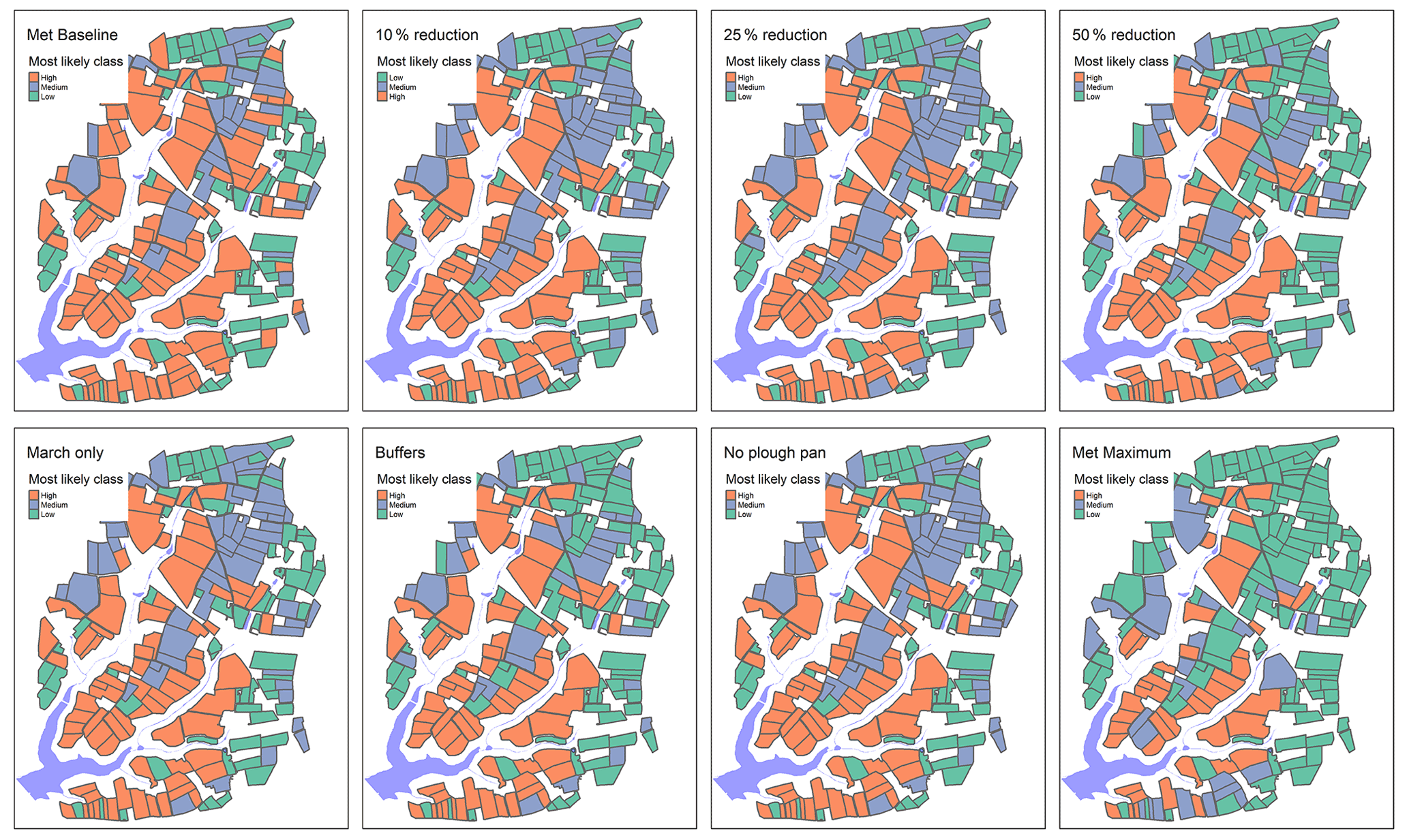
Figure 8Example output showing the most likely overland flow risk class for each field for metobromuron under current (baseline) application practices; with a 10 %, 25 %, or 50 % reduction in application; with a time shift of application to March; with additional field buffers; with no plough pan; and with a combination of all available mitigation measures (shifting application to March, a 50 % reduction in application rates, buffers, and no soil pan).
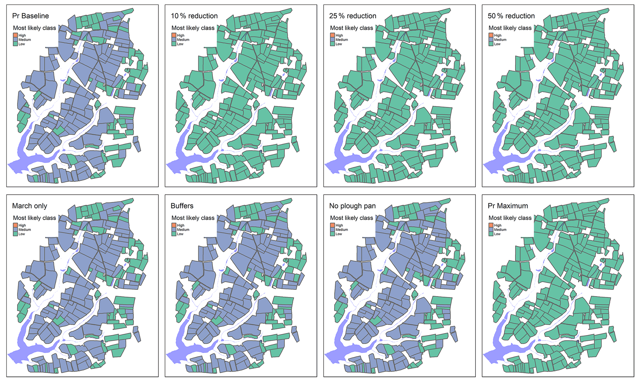
Figure 9Example output showing the most likely groundwater leaching risk class for each field for prosulfocarb under current (baseline) application practices; with a 10 %, 25 %, or 50 % reduction in application; with a time shift of application to March; with additional field buffers; with no plough pan; and with a combination of all available mitigation measures (shifting application to March, a 50 % reduction in application rates, buffers, and no soil pan).
3.4 Model validation
We constructed a causal network, where the model structure was informed by expert knowledge. However, Bayesian networks can also be used as machine learning associative tools that are suitable for deriving patterns in data sets without a specific response variable. It could be argued that pesticide risk, expressed as load or concentration of pesticide in different potential loss pathways (overland flow or groundwater leaching), is a latent variable without available observational data (Piffady et al., 2020), making it difficult to calibrate or validate a risk model. Hence, model credibility and salience (Cash et al., 2005) need to be evaluated by experts and stakeholders. Here, we implemented a simple validation approach to confirm that the model predictions fall within the realms of credibility, using the limited observational data to validate the expert-based model.
Figure 10 shows a comparison between the probability density distributions based on 10 000 surface water risk simulations for each active ingredient in the hybrid network and the limited observational data (in µg L−1) available for the months from January to March between 2016 and 2019. The model typically overestimates the simulated risk for glyphosate and pendimethalin, albeit with low probability of high values. The simulated and observed distributions for prosulfocarb are comparable, whilst the model seems to underestimate the risk from metobromuron. However, it has to be noted that the very few observations available for metobromuron (N=8) seem to be higher and less accurate than for the other pesticides. It should also be noted that the developed model was never intended to represent the complex transport and fate processes in the catchment in detail nor to accurately simulate the pesticide concentration levels in the reservoir, so the comparison in Fig. 10 was mainly carried out as a sense check of the model predictions. Overall, model simulations appear conservative, which is helpful in terms of informing a precautionary management approach. Further model refinement could focus on constraining the upper simulation values throughout the model. A qualitative “reasonable fit” visual inspection has been shown to be an effective means of assessing model performance using diverse incomplete data sets (Ghahramani et al., 2020). Ghahramani et al. (2020) found that the ranking of confidence in model predictions between determinands was related to data availability as much as to the model itself, with pesticide simulations performing less well than those for hydrology, sediments, and phosphorus.
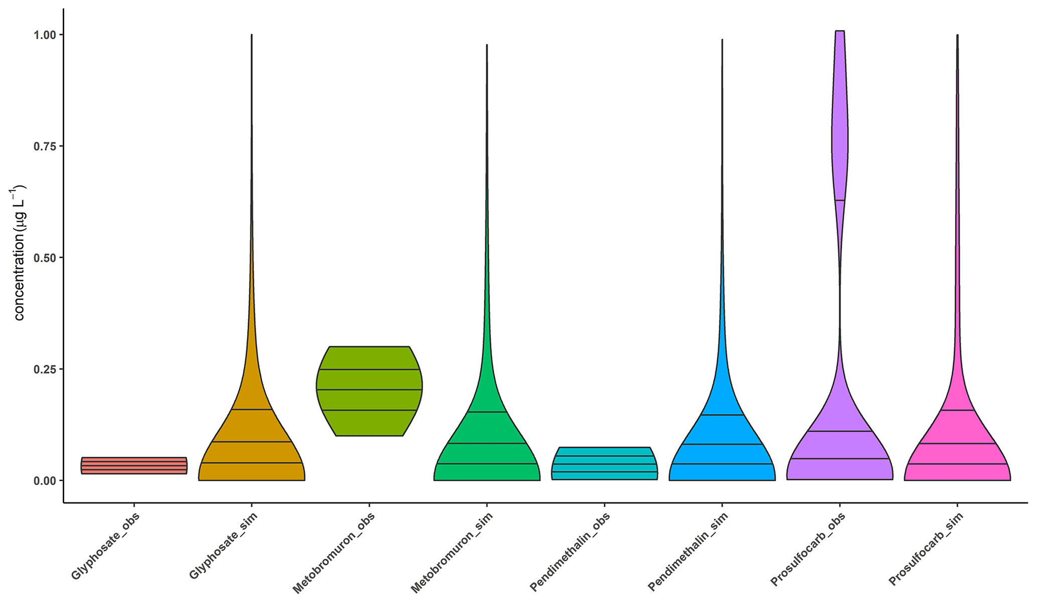
Figure 10Violin plots showing the probability density distribution and three quartiles (25th, 50th, and 75th) of simulated (N= 10 000 iterations) vs. observed (glyphosate N=20, metobromuron N=8, pendimethalin N=73, and prosulfocarb N=25) concentrations for four active ingredients.
Further validation approaches could be explored in future implementations. The spatial application in the bnspatial R package allows one to simulate expected quantities based on the median value of each discretisation interval. Hence, by multiplying the expected loads from each field by the probability of the field falling into each discretised interval, summing the resulting pesticide masses over all fields in the catchment, and then dividing by the reservoir volume, a concentration in the reservoir water could be estimated for each pesticide and month. This could then be compared to measured concentrations, if available, for further model validation. However, this deterministic calculation would be heavily reliant on the discretisation of the target node in question and, coupled with rare extreme high values generated by the stochastic model, would make the validation uncertain. Hence, it would be best applied in combination with dynamic discretisation, if available, and with further model development constraining upper simulated values.
3.5 Limitations and outlook
A unique advantage of BBNs is their ability to inform probabilistic decisions on the basis of incomplete data (Panidhapu et al., 2020) and address “what if” counterfactual scenarios (Gibert et al., 2018; Moe et al., 2021) as well as their ability to integrate data of different quality from different sources and disciplines. In machine learning, the selected mathematical approach needs to be based on the target question to be answered and be aligned with the properties of the available data (Gibert et al., 2018). This study presents a novel approach to pesticide risk analysis that matches the question at hand in a poorly monitored, data-sparse drinking water catchment.
The BBN model could easily be extended to consider other pesticides by changing the pesticide-specific properties, whereas greater structural changes would be needed to simulate the cumulative risk from total pesticide concentrations. However, the developed BBN also has several limitations, and there are various input parameters and elements that could be refined and improved. The BBN only focuses on aquatic risks resulting from the intentional application of pesticide in agriculture and does not consider potential point sources of pesticide contamination (such as misuse, accidental spillage, disposal of pesticides, or cleaning of application equipment). Although quite detailed in process representation that is based on established mechanistic approaches, the modelling of pesticide leaching and runoff in the BBN is still simplified and could be extended, for example, to consider factors such as preferential flow pathways and/or to capture the slower rate of groundwater pesticide leaching as compared with fluxes via surface runoff. Soil water balance and hydrology are critical for pesticide risk assessments, the details of which are challenging to capture with a BBN or an index-based model. Hence, future developments of the approach could include the development of an improved probabilistic soil hydrology model linked to the pesticide risk model.
Discretisation is recognised as a major limitation of BBNs (Nojavan et al., 2017). Whilst we constructed a hybrid network here that has largely allowed us to avoid the loss of information associated with discretisation, this advantage was lost in the spatial application, where existing mathematical and software limitations prevent direct coupling of a hybrid network with GIS. We suggest that this limitation could be an interesting and fruitful avenue for further research and methodological development, for example, by developing software applications that allow automated dynamic discretisation (Fenton and Neil, 2013) coupled with GIS. Finally, the model could be further validated in a highly monitored experimental catchment, thereby also allowing the evaluation of the model transferability.
Notwithstanding the above limitations, this modelling approach satisfies many of the requirements of an “ideal” model to support environmental decision-making, as set out by Schuwirth et al. (2019), in that it “can be directly linked to management objectives, predicts effects of management alternatives without bias, includes adequate precision and a correct estimate of prediction uncertainty and is easy to understand”. We also developed the model with the final criterion of “easy transferability in space and time” in mind, and this could be tested in future applications.
In this study, we present a spatial Bayesian belief network (BBN) that simulates inherent pesticide risk to groundwater and surface water quality, identifies critical source areas, and informs field-level pesticide mitigation strategies in a small drinking water catchment with limited observational data. The BBN accounted for the spatial heterogeneity of the surface water risk from pesticides, considering the spatial distribution of soil properties (e.g. texture, organic matter content, and hydrological properties), topographic connectivity (e.g. slope and distance to surface water/depth to groundwater) and agronomic practices; temporal variability of climatic and hydrological processes (e.g. temperature, rainfall, evapotranspiration, and overland and subsurface flow), and uncertainties related to pesticide properties and the effectiveness of management interventions. The risk of pesticide loss via overland flow and leaching to groundwater were simulated for five active ingredients. Overland pesticide pollution risk from overland flow showed clear spatial variability across the study catchment, whereas groundwater leaching risk was more uniform. The effectiveness of mitigation measures, such as the delayed timing of pesticide application, the reduction of application rates, the installation of additional field buffers, and the management of the soil plough pan, on risk reduction were evaluated. Combined intervention (a 50 % reduced pesticide application rate, management of the plough pan, delayed application timing, and field buffer installation) greatly reduced the probability of high risk from overland flow. The advantages of the presented BBN approach over traditional index-based methods include its ability to integrate diverse data sources (both qualitative and quantitative) for a field-scale assessment of critical source areas of pesticide pollution in a data-sparse catchment, with explicit representation of uncertainties. The graphical nature of the decision support tool facilitates interactive model development and evaluation with stakeholders to build model credibility, while its flexible and dynamic nature allows one to perform both predictive and diagnostic reasoning based on observations, which can be linked to spatially explicit data, thereby improving pesticide risk management.
Table A1The definition of model variables included in the Bayesian belief network, the definition of states and boundaries, and the information and assumptions used to populate prior probabilities or conditional probability tables for each node.
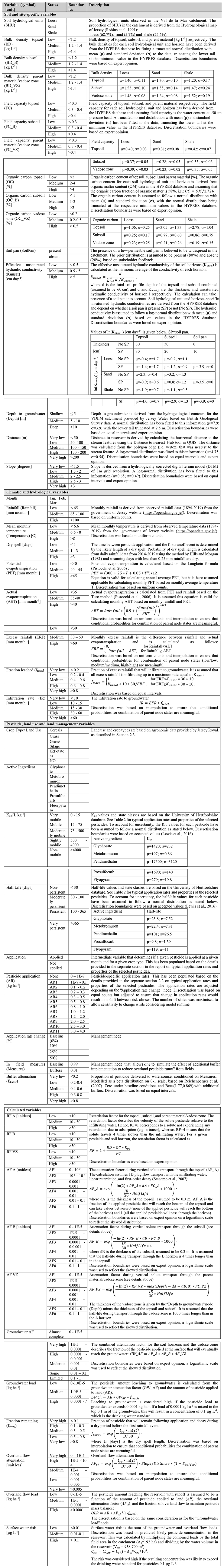
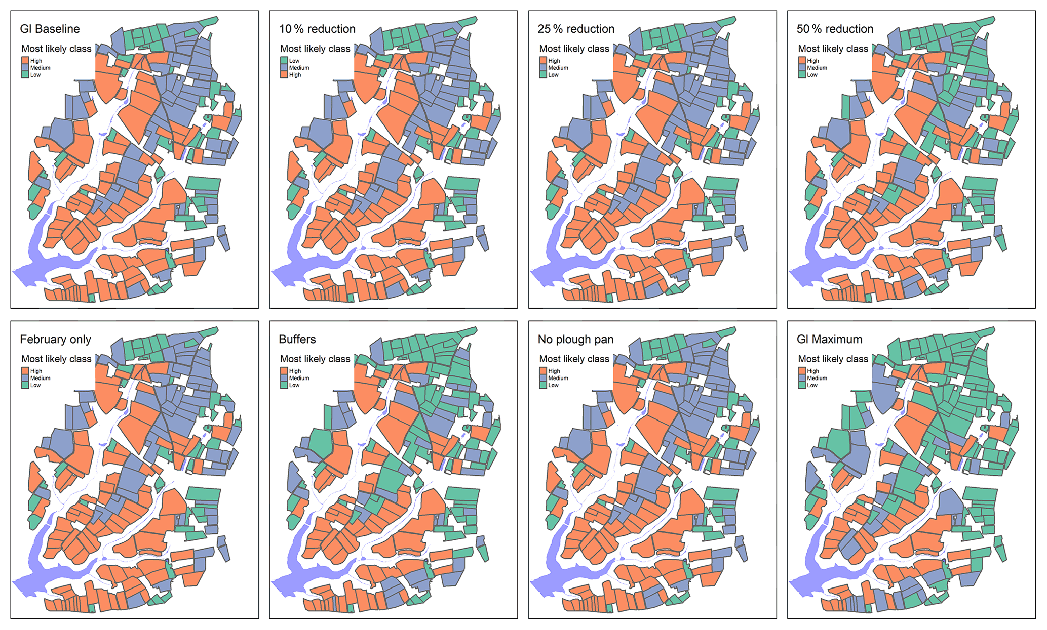
Figure B1Most likely overland flow risk class for glyphosate under current application practices; with a 10 %, 25 %, or 50 % reduction in the application rate; with a time shift of application to February; with additional field buffers; with no plough pan; and with all mitigation measures combined.

Figure B2Most likely overland flow risk class for pendimethalin under current application practices; with a 10 %, 25 %, or 50 % reduction in the application rate; with a time shift of application to March; with additional field buffers; with no plough pan; and with all mitigation measures combined.

Figure B3Most likely overland flow risk class for prosulfocarb under current application practices; with a 10 %, 25 %, or 50 % reduction in the application rate; with a time shift of application to March; with additional field buffers; with no plough pan; and with all mitigation measures combined.
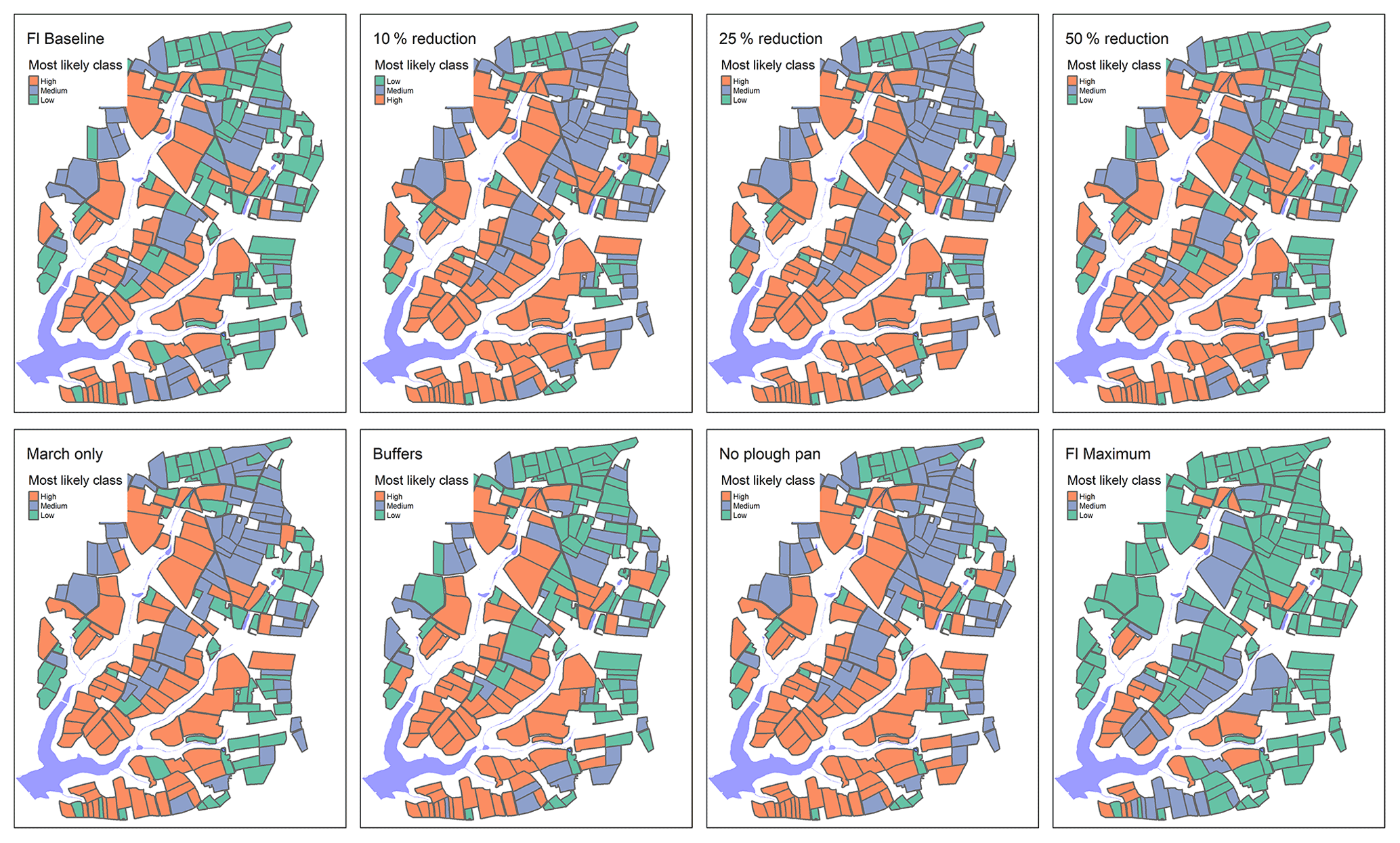
Figure B4Most likely overland flow risk class for fluopyram under current application practices; with a 10 %, 25 %, or 50 % reduction in the application rate; with a time shift of application to March; with additional field buffers; with no plough pan; and with all mitigation measures combined.
The code and data cannot not be made publicly available due to funder restrictions and privacy concerns. However, they may be made available on request by contacting the Operations Director, Jersey Water, Mulcaster House, Westmount Road, St. Helier, JE1 1DG Jersey, UK.
MG led conceptualisation, funding acquisition, and project administration; MT, AL, ZG, and AV undertook formal data analysis; MG and MT led model development and manuscript preparation; ZG led data curation and visualisation. All authors contributed to the methodological development, manuscript review, and editing.
The contact author has declared that neither they nor their co-authors have any competing interests.
Publisher's note: Copernicus Publications remains neutral with regard to jurisdictional claims in published maps and institutional affiliations.
This article is part of the special issue “Frontiers in the application of Bayesian approaches in water quality modelling”. It is a result of the EGU General Assembly 2020, 3–8 May 2020.
We thank the editor, the two referees, and Jannicke Moe from the Norwegian Institute for Water Research for detailed comments on the paper. This research was funded by the Jersey Water Company Ltd.
This research has been supported by the Jersey Water Company Ltd.
This paper was edited by Ibrahim Alameddine and reviewed by two anonymous referees.
Aguilera, P. A., Fernandez, A., Fernandez, R., Rumi, R., and Salmeron, A.: Bayesian networks in environmental modelling, Environ. Modell. Softw., 26, 1376–1388, https://doi.org/10.1016/j.envsoft.2011.06.004, 2011.
Aller, L., Bennet, T., Leher, J. H., Petty, R. J., and Hackett, G.: DRASTIC: a standardized system for evaluating ground water pollution potential using hydrogeological settings, EPA, 641 pp., 1987.
Babaei, H., Nazari-Sharabian, M., Karakouzian, M., and Ahmad, S.: Identification of critical source areas (CSAs) and evaluation of best management practices (BMPs) in controlling eutrophication in the Dez River basin, Environments, 6, 1–15, https://doi.org/10.3390/environments6020020, 2019.
Bereswill, R., Streloke, M., and Schulz, R.: Risk mitigation measures for diffuse pesticide entry into aquatic ecosystems: proposal of a guide to identify appropriate measures on a catchment scale, Integr. Environ. Assess., 10, 286–298, https://doi.org/10.1002/ieam.1517, 2014.
Beven, K., Asadullah, A., Bates, P., Blyth, E., Chappell, N., Child, S., Cloke, H., Dadson, S., Everard, N., Fowler, H. J., Freer, J., Hannah, D. M., Heppell, K., Holden, J., Lamb, R., Lewis, H., Morgan, G., Parry, L., and Wagener, T.: Developing observational methods to drive future hydrological science: Can we make a start as a community?, Hydrol. Process., 34, 868–873, https://doi.org/10.1002/hyp.13622, 2019.
Carriger, J. F. and Newman, M. C.: Influence diagrams as decision-making tools for pesticide risk management, Integr. Environ. Assess., 8, 339–350, https://doi.org/10.1002/ieam.268, 2012.
Carriger, J. F., Barron, M. G., and Newman, M. C.: Bayesian Networks Improve Causal Environmental Assessments for Evidence-Based Policy, Environ. Sci. Technol., 50, 13195–13205, https://doi.org/10.1021/acs.est.6b03220, 2016.
Carriger, J. F., Yee, S. H., and Fisher, W. S.: Assessing Coral Reef Condition Indicators for Local and Global Stressors Using Bayesian Networks, Integr. Environ. Assess., 17, 165–187, https://doi.org/10.1002/ieam.4368, 2021.
Cash, D., Clark, W. C., Alcock, F., Dickson, N., Eckley, N., and Jäger, J.: Salience, Credibility, Legitimacy and Boundaries: Linking Research, Assessment and Decision Making, SSRN Electron. J., John F. Kennedy School of Government Harvard University Faculty Research Working Papers Series, RWP02-046, 25 pp., https://doi.org/10.2139/ssrn.372280, 2005.
Doody, D. G., Archbold, M., Foy, R. H., and Flynn, R.: Approaches to the implementation of the Water Framework Directive: Targeting mitigation measures at critical source areas of diffuse phosphorus in Irish catchments, J. Environ. Manage., 93, 225–234, https://doi.org/10.1016/j.jenvman.2011.09.002, 2012.
Drewry, J. J., Newham, L. T. H., and Greene, R. S. B.: Index models to evaluate the risk of phosphorus and nitrogen loss at catchment scales, J. Environ. Manage., 92, 639–649, https://doi.org/10.1016/j.jenvman.2010.10.001, 2011.
Duttagupta, S., Mukherjee, A., Das, K., Dutta, A., Bhattacharya, A., and Bhattacharya, J.: Groundwater vulnerability to pesticide pollution assessment in the alluvial aquifer of Western Bengal basin, India using overlay and index method, Geochemistry, 80, 125601, https://doi.org/10.1016/j.chemer.2020.125601, 2020.
ESRI: ArcGIS Desktop: Release 10.1, Environmental Systems Research Institute, Redlands, CA, USA, 2011.
European Commission: Council Directive 98/83/EC on the quality of water intended for human consumption, L330, 32–54, https://eur-lex.europa.eu/eli/dir/1998/83/oj (last access: 24 February 2022), 1998.
European Commission: Directive 2000/60/EC of the European Parliament and of the Council of 23 October 2000 establishing a framework for Community action in the field of water policy, Official Journal of the European Communities, L327, 1–72, 2000.
European Commission: Directive 2006/118/EC, Groundwater Directive, Official Journal of the European Union, L372, 19–31, 2006.
European Soil Bureau Network: Soil Atlas of Europe, edited by: Jones, A., Montanerella, L., and Jones, R., 128 pp., Office for Official Publications of the European Communities, Luxembourg, ISBN 928948120X, 2005.
Fenton, N. and Neil, M.: Risk Assessment and Decision Analysis with Bayesian Networks, CRC Press Taylor and Francis, Boca Raton, Florida, USA, 2013.
Fomsgaard, I. S.: Degradation of pesticides in subsurface soils, unsaturated zone – a review of methods and results, Int. J. Environ. An. Ch., 58, 231–245, 1995.
Ghahramani, A., Freebairn, D. M., Sena, D. R., Cutajar, J. L., and Silburn, D. M.: A pragmatic parameterisation and calibration approach to model hydrology and water quality of agricultural landscapes and catchments, Environ. Modell. Softw., 130, 104733, https://doi.org/10.1016/j.envsoft.2020.104733, 2020.
QGIS Development Team: QGIS Geographic Information System, https://www.qgis.org, last access: 24 February 2022.
Gibert, K., Izquierdo, J., Sanchez-Marre, M., Hamilton, S. H., Rodriguez-Roda, I., and Holmes, G.: Which method to use? An assessment of data mining methods in Environmental Data Science, Environ. Modell. Softw., 110, 3–27, https://doi.org/10.1016/j.envsoft.2018.09.021, 2018.
Grauso, S., Pasanisi, F., and Tebano, C.: Assessment of a simplified connectivity index and specific sediment potential in river basins by means of geomorphometric tools, Geosciences, 8, 48, https://doi.org/10.3390/geosciences8020048, 2018.
Guo, K., Zhang, X., Kuai, X., Wu, Z., Chen, Y., and Liu, Y.: A spatial bayesian-network approach as a decision-making tool for ecological-risk prevention in land ecosystems, Ecol. Model., 419, 108929, https://doi.org/10.1016/j.ecolmodel.2019.108929, 2020.
Gustafson, D. I.: Groundwater ubiquity score: A simple method for assessing pesticide leachability, Environ. Toxicol. Chem., 8, 339–357, 1989.
Henriksen, H. J., Kjær, J., Brüsh, W., Jacobsen, L. B., Jensen, J. D., Grinderslev, D., and Andersen, P.: Environmental benefits and social cost – An example of combining Bayesian networks and economic models for analysing pesticide management instruments, Nord. Hydrol., 38, 351–371, https://doi.org/10.2166/nh.2007.017, 2007.
Hills, R. C. and Morgan, J. H. T.: Rainfall statistics: An interactive approach to analysing rainfall records for agricultural purposes, Exp. Agric., 17, 1–16, https://doi.org/10.1017/S0014479700011170, 1981.
Jones, R. L., Keen, D. H., Birnie, J. F., and Waton, P. V: Past landscapes of Jersey: Environmental changes during the last ten thousand years, 156 pp., Societe Jersiaise, Jersey, ISBN 10: 0901897183, 1990.
Jury, W. A., Dennis, D. F., and Farmer, W. J.: Evaluation of Pesticide Groundwater Pollution Potential from Standard Indices of Soil-Chemical Adsorption and Biodegradation, J. Environ. Qual., 16, 422–428, 1987.
Kah, M. and Brown, C. D.: Adsorption of ionisable pesticides in soils, in: Reviews of Environmental Contamination and Toxicology, edited by: Ware, G.W. et al., Rev. Environ. Contam. T., 188, 149–217, https://doi.org/10.1007/978-0-387-32964-2_5, 2006.
Kaikkonen, L., Parviainen, T., Rahikainen, M., Uusitalo, L., and Lehikoinen, A.: Bayesian Networks in Environmental Risk Assessment: A review, Integr. Environ. Assess., 17, 62–78, https://doi.org/10.1002/ieam.4332, 2020.
Kjærulff, U. and van der Gaag, L. C.: Making Sensitivity Analysis Computationally Efficient, Proceedings of the Sixteenth Annual Conference on Uncertainty in Artificial Intelligence (UAI 2000), 30 June 2000–3 July 2000, Stanford University, Stanford, CA, USA, 317–325, 2000.
Köhne, J. M., Köhne, S., and Šimůnek, J.: A review of model applications for structured soils: b) Pesticide transport, J. Contam. Hydrol., 104, 36–60, https://doi.org/10.1016/j.jconhyd.2008.10.003, 2009.
Koiter, J. R.: Visualizing Inference in Bayesian Networks, M.Sc. thesis, Faculty of Electrical Engineering, Mathematics, and Computer Science, Department of Man-Machine Interaction, Delft University of Technology, The Netherlands, 2006.
Kookana, R. S., Correll, R. L., and Miller, R. B.: Pesticide impact rating index – A pesticide risk indicator for water quality, Water Air Soil Pollut: Focus, 5, 45–65, https://doi.org/10.1007/s11267-005-7397-7, 2005.
Korb, K. B. and Nicholson, A. E.: Bayesian artificial intelligence, second edn., Computer Science and Data Analysis Series, 491 pp., CRC Press, Baton Rouge, https://doi.org/10.1201/b10391, 2010.
Koszinski, S., Wendroth, O., and Lehfeldt, J.: Field scale heterogeneity of soil structural properties in a moraine landscape of north-eastern Germany, Int. Agrophysics, 9, 201–210, 1995.
Lane, S. N., Reaney, S. M., and Heathwaite, A. L.: Representation of landscape hydrological connectivity using a topographically driven surface flow index, Water Resour. Res., 45, W08423, https://doi.org/10.1029/2008WR007336, 2009.
Lewis, K. A., Tzilivakis, J., Warner, D., and Green, A.: An international database for pesticide risk assessments and management, Hum. Ecol. Risk Assess., 22, 1050–1064, https://doi.org/10.1080/10807039.2015.1133242, 2016.
MAFF: Agricultural land classification of England and Wales – Revised criteria for grading the quality of agricultural land, Ministry of Agriculture, Fisheries and Food, 1988.
Masante, D.: Package “bnspatial”, GitHub [code], http://github.com/dariomasante/bnspatial (last access: 24 February 2022), 2017.
Mentzel, S., Grung, M., Tollefsen, K. E., Stenrød, M., Petersen, K., and Moe, S. J.: Development of a Bayesian network for probabilistic risk assessment of pesticides, bioRxiv [preprint], 2021.05.20.444913, https://doi.org/10.1101/2021.05.20.444913, 2021.
Moe, S. J., Carriger, J. F., and Glendell, M.: Increased Use of Bayesian Network Models has Improved Environmental Risk Assessments, Integr. Environ. Assess., 17, 53–61, https://doi.org/10.1002/ieam.4369, 2021.
Nobre, R. C. M., Rotunno Filho, O. C., Mansur, W. J., Nobre, M. M. M., and Cosenza, C. A. N.: Groundwater vulnerability and risk mapping using GIS, modeling and a fuzzy logic tool, J. Contam. Hydrol., 94, 277–292, https://doi.org/10.1016/j.jconhyd.2007.07.008, 2007.
Nojavan, A. F., Qian, S. S., and Stow, C. A.: Comparative analysis of discretization methods in Bayesian networks, Environ. Modell. Softw., 87, 64–71, https://doi.org/10.1016/j.envsoft.2016.10.007, 2017.
O'Hagan, A.: Probabilistic uncertainty specification: Overview, elaboration techniques and their application to a mechanistic model of carbon flux, Environ. Modell. Softw., 36, 35–48, https://doi.org/10.1016/j.envsoft.2011.03.003, 2012.
Oakley, J.: Package “SHELF”, GitHub [code], https://github.com/OakleyJ/SHELF (last access: 24 February 2022), 2020.
OECD: Annex 2 – Report of Phase 1 of the Aquatic Risk Indicators Project, https://www.oecd.org/chemicalsafety/pesticides-biocides/2078678.pdf (last access: 24 February 2022), 2000.
Okumah, M., Chapman, P. J., Martin-Ortega, J., and Novo, P.: Mitigating agricultural diffuse pollution: Uncovering the evidence base of the awareness-behaviour-water quality pathway, Water, 11, 29, https://doi.org/10.3390/w11010029, 2018.
Pagano, A., Pluchinotta, I., Giordano, R., Petrangeli, A. B., Fratino, U., and Vurro, M.: Dealing with Uncertainty in Decision-Making for Drinking Water Supply Systems Exposed to Extreme Events, Water Resour. Manag., 32, 2131–2145, https://doi.org/10.1007/s11269-018-1922-8, 2018.
Panidhapu, A., Li, Z., Aliashrafi, A., and Peleato, N. M.: Integration of weather conditions for predicting microbial water quality using Bayesian Belief Networks, Water Res., 170, 115349, https://doi.org/10.1016/j.watres.2019.115349, 2020.
Piffady, J., Carluer, N., Gouy, V., le Henaff, G., Tormos, T., Bougon, N., Adoir, E., and Mellac, K.: ARPEGES: A Bayesian Belief Network to Assess the Risk of Pesticide Contamination for the River Network of France, Integr. Environ. Assess., 17, 188–201, https://doi.org/10.1002/ieam.4343, 2020.
Pistocchi, A., Pilar, V., and Pennington, D.: Analysis of Landscape and Climate Parameters for Continental Scale Assessment of the Fate of Pollutants, European Commission, Directorate-General, Joint Research Centre, Institute for Environment and Sustainability, EUR 22624, 1–109, ISBN 927904809, 2006.
Quaglia, G., Joris, I., Broekx, S., Desmet, N., Koopmans, K., Vandaele, K., and Seuntjens, P.: A spatial approach to identify priority areas for pesticide pollution mitigation, J. Environ. Manage., 246, 583–593, https://doi.org/10.1016/j.jenvman.2019.04.120, 2019.
R Core Team: R: A language and environment for statistical computing, R Foundation for Statistical Computing, Vienna, Austria, https://www.R-project.org/ (last access: 24 February 2022), 2019.
Reaney, S. M., Lane, S. N., Heathwaite, A. L., and Dugdale, L. J.: Risk-based modelling of diffuse land use impacts from rural landscapes upon salmonid fry abundance, Ecol. Model., 222, 1016–1029, https://doi.org/10.1016/j.ecolmodel.2010.08.022, 2011.
Reaney, S. M., Mackay, E. B., Haygarth, P. M., Fisher, M., Molineux, A., Potts, M., and Benskin, C. M. W. H.: Identifying critical source areas using multiple methods for effective diffuse pollution mitigation, J. Environ. Manage., 250, 109366, https://doi.org/10.1016/j.jenvman.2019.109366, 2019.
Reichenberger, S., Bach, M., Skitschak, A., and Frede, H. G.: Mitigation strategies to reduce pesticide inputs into ground- and surface water and their effectiveness; A review, Sci. Total Environ., 384, 1–35, https://doi.org/10.1016/j.scitotenv.2007.04.046, 2007.
Robins, N. S. and Smedley, P. L.: Hydrogeological and hydrochemical survey of Jersey, British Geological Survey Technical Report WD/91/15, British Geological Survey, Keyworth, Nottingham, 101 pp., https://www.gov.je/SiteCollectionDocuments/Environment%20and%20greener%20living/R%20Hydrogeological%20Report.pdf (last access: 24 February 2022), 1991.
Robins, N. S. and Smedley, P. L.: The Jersey groundwater study, British Geological Survey Research Report RR/98/5, British Geological Survey, Keyworth, Nottingham, 48 pp., 1998.
Robins, N. S., Smedley, P. L., and MacDonald, D. M. J.: Hydrogeological map of Jersey, Scale 1:25000, British Geological Survey, Keyworth, Nottingham, 1991.
Saha, D. and Alam, F.: Groundwater vulnerability assessment using DRASTIC and Pesticide DRASTIC models in intense agriculture area of the Gangetic plains, India, Environ. Monit. Assess., 186, 8741–8763, https://doi.org/10.1007/s10661-014-4041-x, 2014.
Sahlin, U., Helle, I., and Perepolkin, D.: “This Is What We Don't Know”: Treating Epistemic Uncertainty in Bayesian Networks for Risk Assessment, Integr. Environ. Assess., 17, 221–232, https://doi.org/10.1002/ieam.4367, 2021.
Schuwirth, N., Borgwardt, F., Domisch, S., Friedrichs, M., Kattwinkel, M., Kneis, D., Kuemmerlen, M., Langhans, S. D., Martínez-López, J., and Vermeiren, P.: How to make ecological models useful for environmental management, Ecol. Model., 411, 108784, https://doi.org/10.1016/j.ecolmodel.2019.108784, 2019.
Sharp, R., Douglass, J., Wolny, S., Arkema, K., Bernhardt, J., Bierbower, W., Chaumont, N., Denu, D., Fisher, D., Glowinski, K., Griffin, R., Guannel, G., Guerry, A., Johnson, J., Hamel, P., Kennedy, C., Kim, C. K., Lacayo, M., Lonsdorf, E., Mandle, L., Rogers, L., Silver, J., Toft, J., Verutes, G., Vogl, A. L., Wood, S, and Wyatt, K.: InVEST 3.10.2.post17+ug.g0e9e2ef User's Guide, The Natural Capital Project, Stanford University, University of Minnesota, The Nature Conservancy, and World Wildlife Fund, 2020.
Stenemo, F., Ray, C., Yost, R., and Matsuda, S.: A screening tool for vulnerability assessment of pesticide leaching to groundwater for the islands of Hawaii, USA, Pest Manag. Sci., 63, 404–411, https://doi.org/10.1002/ps.1345, 2007.
Tang, X., Zhu, B., and Katou, H.: A review of rapid transport of pesticides from sloping farmland to surface waters: Processes and mitigation strategies, J. Environ. Sci., 24, 351–361, https://doi.org/10.1016/S1001-0742(11)60753-5, 2012.
Villamizar, M. L., Stoate, C., Biggs, J., Morris, C., Szczur, J., and Brown, C. D.: Comparison of technical and systems-based approaches to managing pesticide contamination in surface water catchments, J. Environ. Manage., 260, 110027, https://doi.org/10.1016/j.jenvman.2019.110027, 2020.
Vinten, A. J. A., Loades, K., Addy, S., Richards, S., Stutter, M., Cook, Y., Watson, H., Taylor, C., Abel, C., Baggaley, N., Ritchie, R., and Jeffrey, W.: Reprint of: Assessment of the use of sediment fences for control of erosion and sediment phosphorus loss after potato harvesting on sloping land, Sci. Total Environ., 468–469, 1234–1244, https://doi.org/10.1016/j.scitotenv.2013.10.050, 2014.
Wang, R., Yuan, Y., Yen, H., Grieneisen, M., Arnold, J., Wang, D., Wang, C., and Zhang, M.: A review of pesticide fate and transport simulation at watershed level using SWAT: Current status and research concerns, Sci. Total Environ., 669, 512–526, https://doi.org/10.1016/j.scitotenv.2019.03.141, 2019.
Wauchope, R. D., Yeh, S., Linders, J. B. H. J., Kloskowski, R., Tanaka, K., Rubin, B., Katayama, A., Kördel, W., Gerstl, Z., Lane, M., and Unsworth, J. B.: Pesticide soil sorption parameters: Theory, measurement, uses, limitations and reliability, Pest Manag. Sci., 58, 419–445, https://doi.org/10.1002/ps.489, 2002.
Worrall, F. and Kolpin, D. W.: Direct assessment of groundwater vulnerability from single observations of multiple contaminants, Water Resour. Res., 39, 1345–1352, https://doi.org/10.1029/2002WR001212, 2003.
Wösten, J. H. M., Lilly, A., Nemes, A., and Le Bas, C.: Using existing soil data to derive hydraulic parameters for simulation models in environmental studies and in land use planning. Final report of the EU funded project “Using existing soil data” (CHRX-CT94-0639), 106 pp., DLO Winand Staring Centre for Integrated Land, Soil and Water Research (SC-DLO), Wageningen, The Netherlands, Report 156, ISSN 0927-4537, 1998.
Wosten, J. H. M., Lilly, A., Nemes, A., and Le Bas, C.: Development and use of a database of hydraulic properties of European soils, Geoderma, 90, 169–185, 1999.
- Abstract
- Introduction
- Methods
- Results and discussion
- Conclusions
- Appendix A: Model description
- Appendix B: Results for overland water risk for all pesticides under all scenarios
- Code and data availability
- Author contributions
- Competing interests
- Disclaimer
- Special issue statement
- Acknowledgements
- Financial support
- Review statement
- References