Future water temperature of rivers in Switzerland under climate change investigated with physics-based models

River ecosystems are highly sensitive to climate change and projected future increase in air temperature is expected to increase the stress for these ecosystems. Rivers are also an important socio-economic factor impacting, amongst others, agriculture, tourism, electricity production, and drinking water supply and quality. In addition to changes in water availability, climate change will impact river temperature. This study presents a detailed analysis of river temperature and discharge evolution over the 21st century in Switzerland. In total, 12 catchments are studied, situated both on the lowland Swiss Plateau and in the Alpine regions. The impact of climate change is assessed using a chain of physics-based models forced with the most recent climate change scenarios for Switzerland including low-, mid-, and high-emission pathways. The suitability of such models is discussed in detail and recommendations for future improvements are provided. The model chain is shown to provide robust results, while remaining limitations are identified. These are mechanisms missing in the model to correctly simulate water temperature in Alpine catchments during the summer season. A clear warming of river water is modelled during the 21st century. At the end of the century (2080–2090), the median annual river temperature increase ranges between +0.9 ^∘C for low-emission and +3.5 ^∘C for high-emission scenarios for both lowland and Alpine catchments. At the seasonal scale, the warming on the lowland and in the Alpine regions exhibits different patterns. For the lowland the summer warming is stronger than the one in winter but is still moderate. In Alpine catchments, only a very limited warming is expected in winter. The period of maximum discharge in Alpine catchments, currently occurring during mid-summer, will shift to earlier in the year by a few weeks (low emission) or almost 2 months (high emission) by the end of the century. In addition, a noticeable soil warming is expected in Alpine regions due to glacier and snow cover decrease. All results of this study are provided with the corresponding source code used for this paper.

1 Introduction

River systems are considered to be among the ecosystems most sensitive to climate change (CC) (Watts et al., 2015) and the projected future increase in air temperature (IPCC, 2021) is expected to increase the stress for these ecosystems. Water temperature is one of the most important variables for aquatic ecosystems, influencing both chemical and biological processes (Benyahya et al., 2007; Temnerud and Weyhenmeyer, 2008). Certain fish species are highly sensitive to warm water, which can promote specific diseases (e.g. proliferative kidney disease, PKD) or prevent reproduction (Caissie, 2006; Carraro et al., 2016), while higher temperatures might be favourable for some other species, enhancing biological invasion (Paillex et al., 2017; Niedrist and Füreder, 2021). In Alpine regions, together with water temperature, glacier retreat is also expected to contribute to accelerated changes in ecosystems (Cauvy-Fraunié and Dangles, 2019; Fell et al., 2021).

Hence, river temperature is an important socio-economic factor. The literature clearly identified several vulnerable sectors: agriculture, tourism, electricity production, as well as drinking water supply and quality (e.g. Hock et al., 2005; Barnett et al., 2005; Schaefli et al., 2007; Bourqui et al., 2011; Viviroli et al., 2011; Beniston, 2012; Hannah and Garner, 2015). For example, during the exceptional heat wave and dry period in central and northern Europe from April through to August 2018, local electricity production at the Swiss nuclear power plant Mühleberg, Canton Bern, had to be temporarily reduced due to the unusually high water temperature of the Aare River. Increase in surface water temperature is also expected to affect groundwater temperatures through river water infiltration, with significant consequences for the biochemistry of these reservoirs (Epting et al., 2021).

Several global-scale studies have shown a clear trend in river temperature (Morrison et al., 2002; Webb and Nobilis, 2007; van Vliet et al., 2013; Null et al., 2013; Ficklin et al., 2014; Hannah and Garner, 2015; Watts et al., 2015; Santiago et al., 2017; Dugdale et al., 2018; Jackson et al., 2018) as well as in lake surface temperature (Dokulil, 2014; O'Reilly et al., 2015; Woolway and Merchant, 2017; Woolway et al., 2020a, b) at various locations over the last decades. For Switzerland, a recent study found a mean increase in river temperature of 0.33±0.03 ^∘C per decade between 1980 and 2018, which is associated with an increase in air temperature (Michel et al., 2020). This study also showed that the response to CC in Alpine catchments is different from those on the Swiss Plateau (lowland). So far, the warming rate of rivers in Swiss Plateau catchments has been almost twice that of Alpine catchments. Studies investigating the future evolution of water temperature in Switzerland are sparse and cover only a few catchments (see e.g. CH2011, 2011; Råman Vinnå et al., 2018).

For all the above reasons, quantitative information on the future evolution of river temperature is necessary. River temperature is expected to be affected by CC mainly through the influence of rising air temperature, changes in precipitation, and changes in snowmelt and ice melt. To simulate the future river temperature evolution, a wide range of existing hydrological models is available. Systematic reviews of such models exist in the literature (e.g. Benyahya et al., 2007; Gallice et al., 2015). These models are generally divided into two main families: statistical and physics-based models. Statistical models might not be valid outside of the observed temperature range, which is an important drawback in the case of CC studies (Benyahya et al., 2007; Leach and Moore, 2019). In addition, a more physics-based representation of the snow- and ice-related processes in space and time, despite usually requiring more input data, allows for improved snow-runoff modelling during the snowmelt season, which is crucial in Alpine catchments (Martin and Etchevers, 2005; Magnusson et al., 2011; Lisi et al., 2015; Brauchli et al., 2017; Du et al., 2021; Carletti et al., 2021). Therefore, a physics-based model approach was chosen.

The present study has two main objectives: (i) assess the ability of a physics-based model chain to simulate discharge and water temperature. This is achieved by using performance metrics over calibration and validation periods and by assessing how far the models are able to reproduce currently observed trends. (ii) Investigate the impact of CC on river temperature. Despite the existence of extensive recent studies on discharge evolution under CC in Switzerland over a larger set of catchments (Brunner et al., 2019a, b; Muelchi et al., 2021a, b), discharge is included in our analysis given the coupling of water temperature and discharge. For both objectives, the comparison of lowland versus Alpine catchments is one of the focal points of this research.

The focus is on Switzerland, a country presenting a wide topographic heterogeneity leading to different discharge and thermal regimes between the lowland Swiss Plateau regions, where the hydrological cycle is mainly precipitation driven, and the high-altitude Alpine regions, where snowmelt and glacier melt play an important role.

We use the snowmelt and runoff model Alpine3D (Lehning et al., 2006) coupled to the semi-distributed hydrological model StreamFlow (Gallice et al., 2016). This model chain has already been successfully applied in Alpine discharge modelling studies by Comola et al. (2015), Wever et al. (2017), Brauchli et al. (2017), and Griessinger et al. (2019).

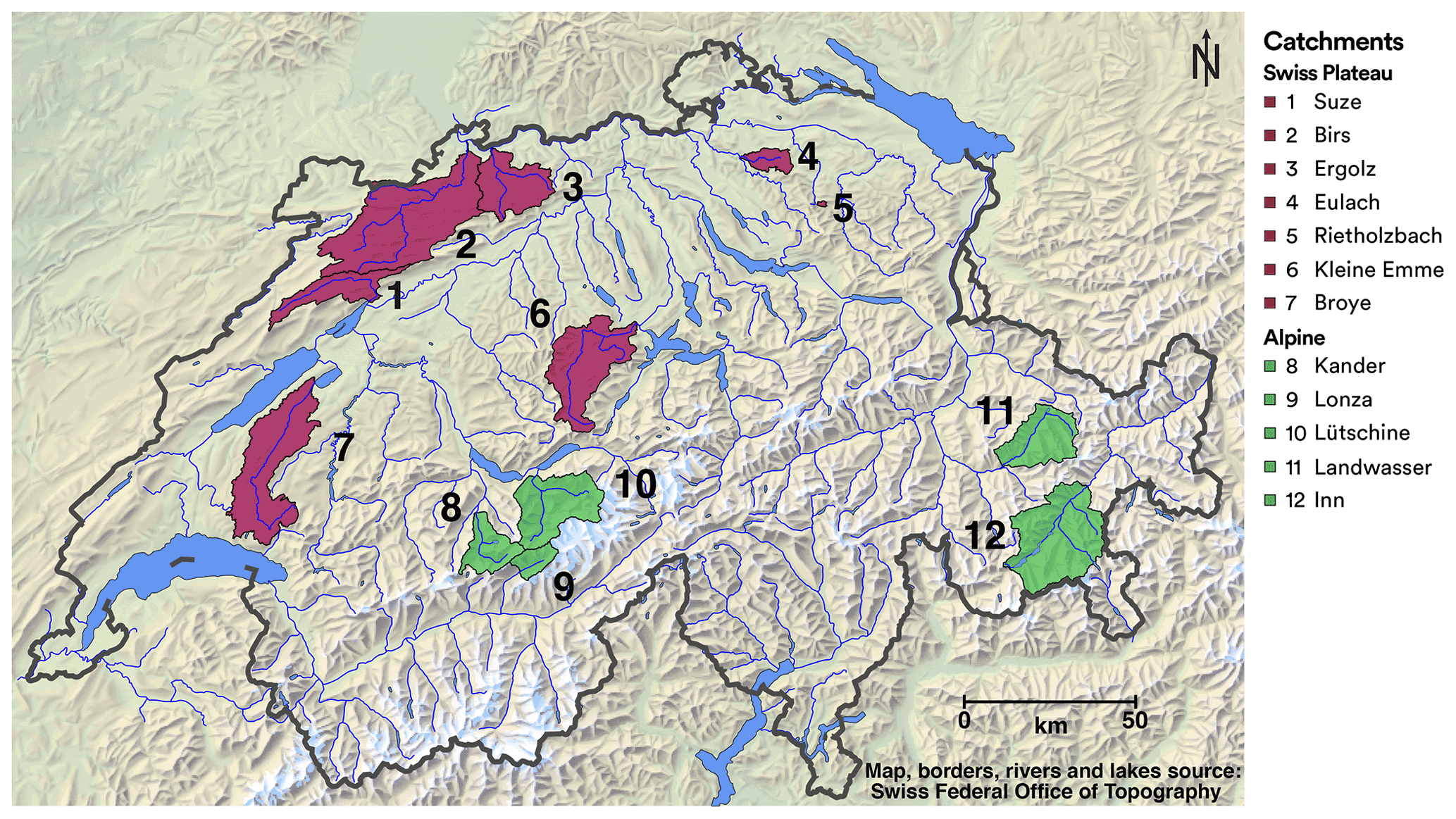
Figure 1 Map of Switzerland showing the location of the simulated catchments. Maps providing details of individual catchments are shown in Fig. S1. Data source: Swiss Federal Office of Topography (Swisstopo).

2 Data

2.1 Catchments

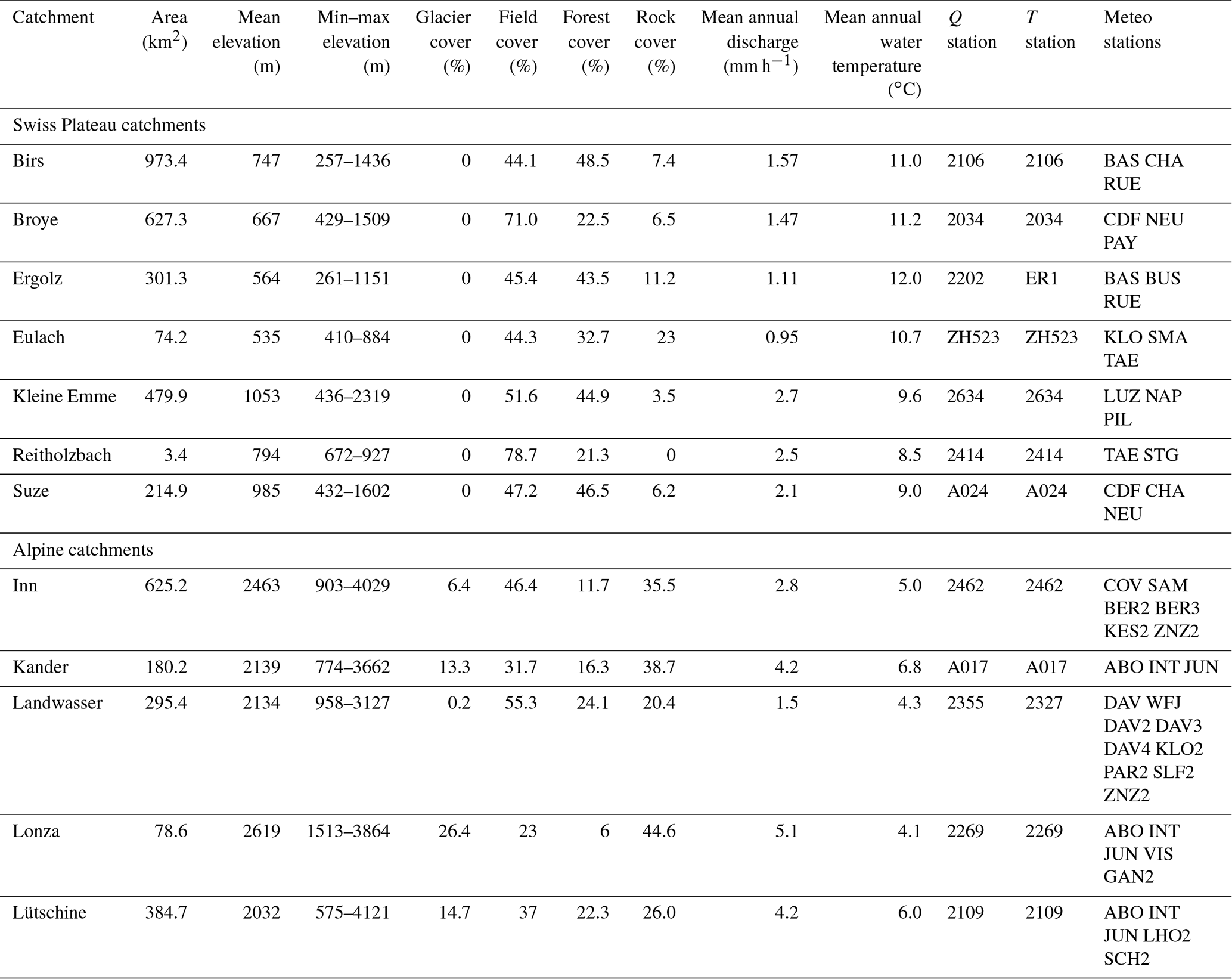
For this study, 12 catchments are selected; they are shown in Fig. 1 and their characteristics are listed in Table 1. They cover a wide range of catchment sizes (from 3.4 to 973 km²). The objective is to include representative catchments both on the Swiss Plateau and in the Swiss Alps. Further selection is based on the availability of hydrological and meteorological measurements as well as CC scenarios. Other selection criteria are minimal anthropogenic disturbances and absence of larger lakes along the watercourse since the models do not take into account these effects (Sect. 3.3). Dams being very abundant in Switzerland (Belletti et al., 2020; Mulligan et al., 2020), the choice of Alpine catchments to be simulated is rather limited, resulting in the set of Inn, Kander, Landwasser, Lonza, and Lütschine catchments.

Table 1 Details of the selected catchments. Details of land cover are given in Sects. 2.5 and S3; built-up areas are treated as rock. Details of discharge stations (Q stations) and water temperature stations (T stations) are given in Table S1. Details of meteorological stations are given in Table S2. Mean annual water temperature and discharge are given at the gauging stations, which do not necessarily correspond to the outlets simulated with CC scenarios (see text); they are computed over the period 2005–2015, except for the Ergolz (2014–2018).

For the Swiss Plateau, more catchments satisfy the requirements. Considering a range of catchment sizes, the following catchments are retained: Birs, Broye, Ergolz, Eulach, Kleine Emme, Rietholzbach, and Suze. This selection is also based on the use of those catchments for groundwater studies (Epting et al., 2021).

For some catchments, the simulations are extended further downstream of the hydrological gauging station being used for calibration to allow for connection to lakes and for the use of the simulation results in a related groundwater study of Epting et al. (2021). A detailed map showing the topography, catchment boundaries, stream network, and locations of hydrological and meteorological stations for each catchment is shown in Fig. S1 in the Supplement.

2.2 Hydrological data

Quality-controlled water temperature and discharge measurements at hourly resolution are provided by the Federal Office for the Environment, FOEN (FOEN, 2019), the Office for Water and Waste of the Canton of Bern, AWA (AWA, 2019), the Office for Waste, Water, Energy and Air of the Canton of Zurich, AWEL (AWEL, 2019), and Holinger AG. Details of the hydrological stations used are given in Table S1 and Fig. S1 in the Supplement.

2.3 Meteorological data

Meteorological data used in this study are provided by the MeteoSwiss (MCH) automatic monitoring network, distributed through IDAWEB (2020), and by the Inter-Cantonal Measurement and Information System (IMIS, 2019). Each catchment is simulated using forcing data from two to nine IMIS and/or MCH stations, depending on the number of available stations within or nearby the catchment (for details, see Tables 1 and S2 and Fig. S1). The variables used at hourly resolution to force the model are air temperature (TA), precipitation accumulation (PSUM), wind velocity (VW), relative humidity (RH), and incoming shortwave radiation (ISWR). Only variables that are available at measurement stations and in the downscaled CH2018 CC scenarios dataset (see Sect. 2.4) are used to ensure that the historical and CC model runs use the exact same set of forcing data.

Note that IMIS stations do not measure ISWR; they are also not equipped with heated precipitation gauges. For these stations, precipitation is deduced from snow depth variations during the winter season using the snow settling calculated by the SNOWPACK model (Lehning et al., 2002b) and from interpolation of nearby MCH stations with heated rain gauges in case of the absence of snow.

Incoming longwave radiation (ILWR), required to force the models, is measured at some MCH stations. However, this variable is not included in the CH2018 dataset used to force the model during CC simulations. As a consequence, for both historical and CC periods, ILWR is calculated at the location of the meteorological stations applying an “all-sky” approach described in Omstedt (1990), which uses TA, RH, and ISWR to estimate the cloud cover fraction and the longwave downward radiation. Methods used for interpolating the input data are described in Sect. 3.2.

2.4 Climate change scenarios

Recent climate change scenarios are available for Switzerland from the CH2018 dataset (NCCS, 2018) at daily resolution, based on the European Coordinated Regional Climate Downscaling Experiment, EURO-CORDEX. Since detailed physics-based snow models require sub-daily granularity, a downscaled version of this dataset at hourly resolution and at station scale is used (Michel et al., 2021a, b). This dataset also includes an extension of the CH2018 scenarios to the IMIS station network. The temporal downscaling is performed using an improved delta change approach which is shown to correctly preserve the seasonal means of the CC scenarios. Since this method requires longer historical time series than the procedure used to derive the CH2018 scenarios, some stations had to be excluded from the original dataset. In addition, the used downscaling method requires the results to be analysed at a monthly or seasonal scale, since shorter time periods may not be correctly captured (see discussion in Michel et al., 2021b).

Most IMIS stations were installed after 2000, entailing that only 10-year periods of downscaled CC scenarios can be constructed. For all IMIS stations, the temporally downscaled dataset for CC scenarios is computed for each individual decade between 1990 and 2100. For the MCH stations, which generally have much longer data availability, scenarios for 30-year periods between 1980 and 2100 were also constructed in addition to the 10-year periods. Using the time series derived over 30 years would be beneficial since 30-year periods are generally considered to capture the climatic trends better than 10-year periods (Michel et al., 2021b) and are often the standard length for CC studies (WMO, 2017). However, this would prevent the usage of IMIS stations. Magnusson et al. (2011) and Schlögl et al. (2016) have shown that increasing the number of stations used to force the model indeed improves the simulations over Alpine catchments. Accordingly, we use the 10-year time series in this work. In Sect. S7 we assess the impact of using 10-year versus 30-year periods and show that only the range of warming is impacted, not the median values.

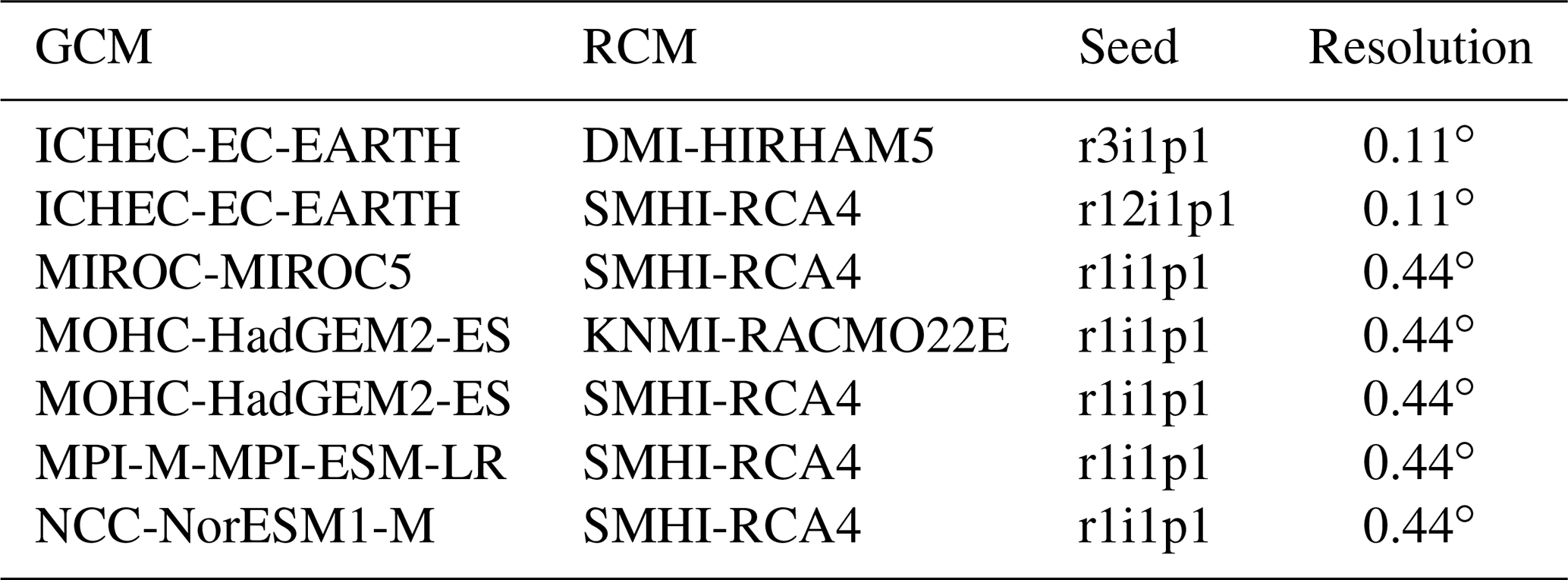
Out of the 68 CC scenarios provided in Michel et al. (2021b), 21 are used in the present study: 7 for the RCP2.6 emission scenarios (low to negative emission), 7 for the RCP4.5 emission scenarios (moderate emission), and 7 for the RCP8.5 scenarios (business as usual). These CC scenarios originate from seven chains of global climate models (GCMs) and regional climate models (RCMs) as detailed in Table 2. Only these seven model chains contain all the variables and RCPs needed for the simulations performed here. The CC simulations are run over the hydrological years 1991–2000, 2006–2015, 2031–2040, 2056–2065, and 2081–2090, referred to as CC periods. For simplicity, we use full decade names further in this paper (e.g. 1990–2000 for the hydrological years 1991–2000, meaning 1 October 1990 to 30 September 2000). The period 2005–2015 is used to validate the CC simulations against measurements for catchments where long-enough historical measurements are available. In the following, the meteorological seasons used for the analysis are abbreviated as follows: winter: DJF (December, January, and February), spring: MAM (March, April, and May), summer: JJA (June, July, and August), and autumn: SON (September, October, and November).

Table 2 Climate change model chains used in this study. For each model chain the RCP2.6, RCP4.5, and RCP8.5 scenarios are used.

2.5 Elevation, glacier, catchment geometry, and land cover data

To perform simulations with Alpine3D, a digital elevation model (DEM) is needed as well as a land use classification to initialize the pixels in the model in an appropriate state and to define the soil and canopy properties. For glaciated catchments, the ice area and thickness need to be provided.

The DEM is derived from the DTM25 dataset at 25 m resolution provided by Swisstopo, averaged to the resolutions used for the simulations (100 and 500 m). Land cover data are derived from the 2006 version of the Copernicus CORINE Land Cover (European Environment Agency, 2013) dataset (CLC) at 100 m resolution (upscaled to 500 m resolution). CLC land cover classes are translated into the land cover classes available in Alpine3D (see Table S3). The catchment and hydrological network, together with sub-catchments attached to each river reach, are derived using the TauDEM software (Tarboton, 1997) with a wrapper to force it to reproduce exactly the river network provided by the Swiss Federal Office for the Environment (FOEN) (Swiss Federal Office for the Environment, 2013, 2020). Details of this method along with an evaluation are given in Sect. S3.

Detailed glacier thickness maps (i.e. ice thickness above bedrock surface) are used at the starting point for each simulation. The evolution of the glacier geometry is simulated with the model GloGEMflow (Zekollari et al., 2019). Details are presented in Sect. 3.1. The glacier maps overwrite the CLC land cover classes and pixels considered to be glacier in CLC but not in the glacier model and are turned into bare rock pixels.

Glacier coverage and mean elevation indicated in Table 1 are obtained from the glacier height grids and DEM described above, which means that they might differ slightly from values given by the data provider for the gauging stations.

3 Models

The models used in this study, GloGEMflow, Alpine3D, and StreamFlow, are presented in detail in Zekollari et al. (2019), Lehning et al. (2006), and Gallice et al. (2016), respectively. Here we only provide a short overview of the models and emphasize aspects relevant for the present application. The main workflow of Alpine3D and StreamFlow is shown in Fig. 2.

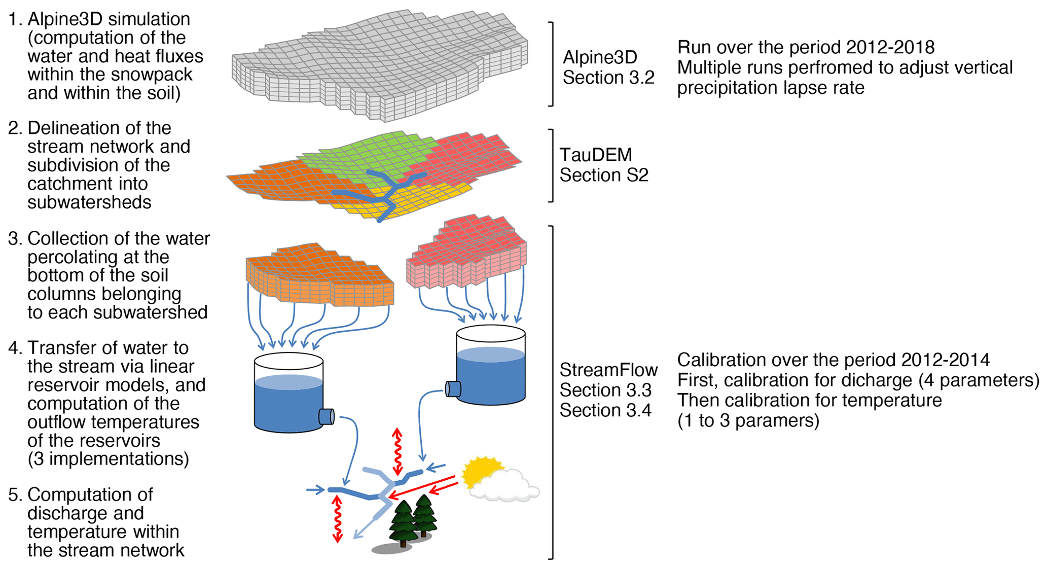
Figure 2 Details of the models' workflow. The calibration and validation periods indicated are valid for all catchments except for the Eulach catchment (where the periods 2015–2016 and 2017–2018 are used instead). Figure adapted from Gallice et al. (2016).

For Alpine3D, as well as for StreamFlow, significant optimization work was necessary in order to use the model chain for such a computationally intensive study. Details of the optimization procedure are presented in Michel (2021).

3.1 GloGEMflow

GloGEMflow calculates the evolution of all individual glaciers along their flowlines by explicitly accounting for both surface mass balance and ice flow processes. The mass balance is calculated from a positive degree-day approach (Huss and Hock, 2015), while ice flow is described through the shallow-ice approximation (Hutter, 1983). GloGEMflow was extensively evaluated over the European Alps by relying on observed mass balances, surface velocities, and glacier changes and by comparing the simulated glacier changes to those from high-resolution 3D modelling studies that focus on individual glaciers (e.g. Jouvet et al., 2009; Zekollari et al., 2014). The simulated glacier extents under the CH2018 CC scenarios considered in this study were transformed from the GloGEMflow 1D model grid to the 2D model grid (at both 100 and 500 m resolution) by ensuring that the area and volume were conserved for each elevation band. This conversion was performed by taking the 2D reference glacier geometry (Huss and Farinotti, 2012) as a starting point and applying a uniform absolute change in ice thickness per elevation band to match the GloGEMflow modelled area. Subsequently, the resulting 2D ice thickness was changed uniformly (same relative change) per elevation band to match the modelled GloGEMflow volume.

3.2 Alpine3D

Alpine3D is a spatially distributed version of the multi-layer snow and soil model SNOWPACK, which explicitly solves the mass and energy balance equations and simulates the snow micro-structure (Lehning et al., 2002b, a). As discussed in the introduction, previous studies have shown the added value of a complex snow model in Alpine environments, while we argue that, for Swiss Plateau regions, such complex models may not be required. However, Alpine3D provides the vertically resolved soil temperature, which is required in StreamFlow and not provided in simpler models. In addition, using Alpine3D throughout allows us to have a consistent land surface model between all catchments. Alpine3D is run at 500 m resolution for all catchments except the small Rietholzbach catchment, where a resolution of 100 m is used. The resolution is chosen to reduce the computational cost, and it has been shown to have only a minor impact on simulated snow depth (Schlögl et al., 2016). The input data for Alpine3D are interpolated to the grids using various algorithms provided by the MeteoIO library (Bavay and Egger, 2014). The air temperature is first de-trended for elevation (using a vertical lapse rate computed from the measurements), then interpolated using inverse distance weighting, and finally re-trended. An analogue procedure is applied for longwave radiation (using a constant lapse rate of −31.25 W m⁻² km⁻¹ to mimic the effect of decreasing air temperature), for wind velocity (using the lapse rate computed from the measurements), and for precipitation, where values of the vertical lapse rate range between 10 % km⁻¹ and 50 % km⁻¹ (see Sect. 3.4). Finally, cloud cover is derived at each meteorological station from ISWR (if available) and interpolated to the grids using an inverse distance weighting algorithm. This cloud cover is then used to adjust the theoretical diffuse and direct radiation at each pixel (Helbig, 2009). Topographical shading is taken into account and a simple model of reflected radiation from surrounding terrain is used.

Alpine3D contains a two-layer canopy module simulating the micro-meteorology in the forest, the evapotranspiration, and the interaction between trees and snow, including snow interception (Gouttevin et al., 2015). Grass, crops, and other land covers are not directly simulated by the canopy module, and the evapotranspiration here is parameterized through the value of the roughness length used in the computation of the latent heat flux. Water infiltration in snow and soil is handled through a simple bucket model. As shown in previous studies, the bucket scheme provides adequate performance on daily and seasonal timescales (Wever et al., 2014, 2015). Alpine3D does not handle partially covered snow pixels, which might delay the melt at the end of the snow season due to overestimated albedo.

Both Alpine3D and StreamFlow are run at hourly resolution. The model writes gridded output for all interpolated forcing variables together with the soil temperature at various depths and the runoff at the bottom of the soil column.

3.3 StreamFlow

StreamFlow is a semi-distributed model concurrently simulating discharge and temperature in each river segment. The runoff at the bottom of the soil column as calculated by Alpine3D is totalized at the scale of each sub-catchment in StreamFlow (see Fig. 2), and the residence time in the soil is determined with an approach using two linear reservoirs in series (Perrin et al., 2003) with reservoir-calibrated coefficients. A parameter representing a fraction of water loss (emulating deep soil infiltration or the difference between surface and sub-surface catchment area) can be calibrated in addition. A single parameter set is calibrated for the entire catchment, with the reservoir parameters being scaled to the sub-catchment size (Gallice et al., 2016).

Based on this sub-catchment runoff, the model uses either a lumped approach (where each stream reach is resolved as a single element, receiving input from its related sub-catchment) or a discretized approach (where reaches are separated into sub-elements based on the resolution used) to compute reach-scale water temperature and runoff routing to the outlet.

For water routing at the reach scale or at the sub-element scale, either an instant routing is considered or a routing scheme based on the Muskingum–Cunge approach, which solves a diffusive-wave approximation of the shallow water equation (Cunge, 1969; Ponce and Changanti, 1994). Regardless of the water routing scheme, heat is explicitly advected together with the mass.

The water temperature in the soil reservoirs at the sub-catchment scale (which determines the water temperature when leaving the reservoirs and entering the river reaches) can be computed in StreamFlow either by (a) using the approach of Comola et al. (2015) based on energy balance between groundwater and soil temperature (where one parameter needs to be calibrated), (b) using the approach of the Hydrological Simulation Program–Fortran, HSPF (Bicknell et al., 1997), or (c) simply taking the soil temperature at a given depth. The HSPF approach essentially approximates the time evolution of the water temperature in the reservoirs by smoothing and adding an offset to the time series of air temperature (the smoothing factor and offset are calibrated parameters). For all three approaches, forcing values averaged over each sub-catchment are used. Different routing and soil water temperature schemes are tested for choosing the most suitable one.

Once the water is routed to the river, the evolution of the water temperature is obtained by computing the energy balance for each reach considering short- and long-wave radiation, sensible and latent heat fluxes, heat exchange and friction with the streambed, and heat advection from upstream reaches and from water input from the stream–hillslope interface. The latent heat flux is computed using a simplified Penman equation (Hannah et al., 2004; Haag and Luce, 2008; Magnusson et al., 2012) and the sensible heat flux is computed from a classical approach (Brown, 1969). The coefficient of heat transfer between the ground and the river needs to be calibrated. Note that the soil depth used for streambed exchange and for the infiltrating water temperature in approaches (a) and (c) is the same. Different depths are tested, and the soil depth leading to the best results is used (Sect. S5 shows that the soil depth chosen for streambed exchange has only a weak impact).

Input data from Alpine3D used in StreamFlow benefit from the treatment performed in Alpine3D, i.e. topographic shading and shading from vegetation present in the land cover dataset used (see Sect. 2.5) combined with the impact of vegetation on wind speed. Small-scale riparian vegetation shading is not accounted for, which might lead to an overestimation of the radiation input in small streams. However, Sect. S9 shows that this has only a minor impact.

3.4 Calibration and validation of models

For the calibration/validation process, Alpine3D is run for the hydrological years 2012–2018. Each Alpine3D simulation is started in July, and the first 3 months serve as spin-up. Before formal parameter calibration in StreamFlow, multiple model runs of Alpine3D are performed with different values of the precipitation vertical lapse rate to adjust the yearly total mass balance in Alpine catchments. In addition, modelled snow heights are compared to measurements to assess the capacity of Alpine3D in reproducing observed snow season dynamics in terms of season duration. Alpine3D has therefore undergone some parameter adjustment but is not calibrated in a strict sense.

After this initial performance check of Alpine3D, StreamFlow is calibrated over the years 2012–2014 and validated over the years 2015–2018. The only exception is the Eulach catchment, where due to the lack of water temperature measurements before 2014, Alpine3D is run over the years 2015–2018, while the calibration and validation periods are 2015–2016 and 2017–2018. Every StreamFlow simulation is run using the first 2 years of data for spin-up and then re-started from the beginning of the time period. Section S4 shows sensitivity tests for the Broye and Lonza catchments using a longer simulation time period (2002–2018). Different calibration periods are used within these 17 years to test for a significant influence on the hydrological model output (Myers et al., 2021), which was not the case.

Depending on the set-up, between five and seven parameters need to be calibrated in StreamFlow (four for discharge and the rest for water temperature; see Table 3). The calibration is performed with a Monte Carlo approach, first for the four parameters of the discharge module (50 000 runs) and then for the parameters of the water temperature module (10 000 runs). The calibration for water temperature is run only for the best parameter set obtained from the discharge calibration and is run with soil temperature calculated by Alpine3D at different depths (the depth leading to the best results being kept; see Sect. S5).

Table 3 Calibration parameters and range of values used in StreamFlow; see Gallice et al. (2016) for details.

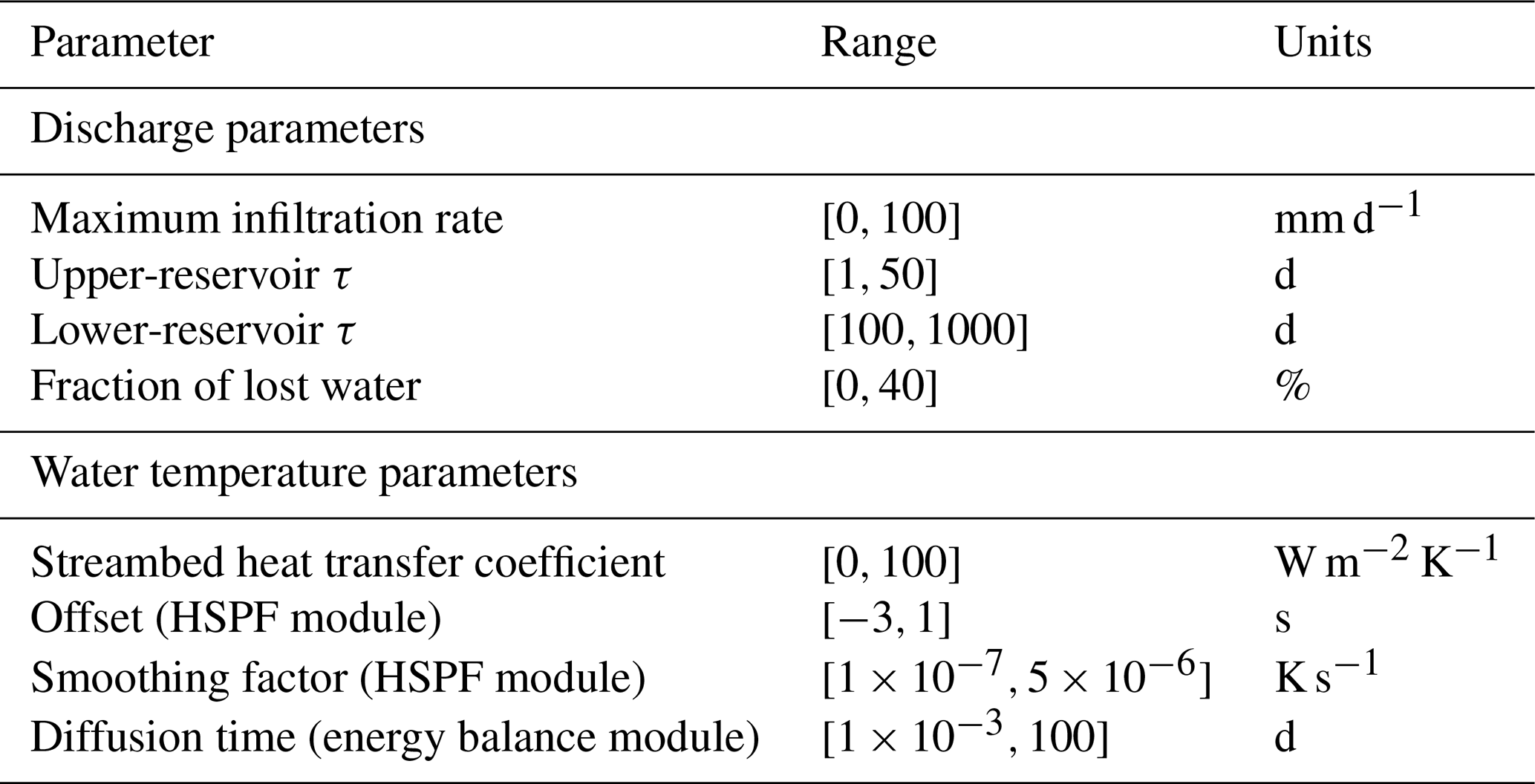
The sequential calibration is motivated by the fact that the model is significantly faster when only discharge is computed. The random sets are drawn from uniform distributions, with bounds indicated in Table 3 (taken and slightly adapted from the work of Gallice et al., 2016). All other model parameters, such as aspect ratio of the reach cross section, are taken from Gallice et al. (2016). As performance metrics, we use the Kling–Gupta efficiency (KGE) coefficient (Gupta et al., 2009) for discharge and the root mean square error (RMSE) for water temperature.

4 Results

4.1 StreamFlow calibration and validation results

Before proper calibration, the performance of the different StreamFlow modules is assessed (see details in Sect. S5). To this end, the calibration is performed using either the lumped or discretized and the direct or Muskingum–Cunge approaches for reach-scale water routing (four combinations) and the three sub-catchment temperature schemes. These are tested at both 100 and 500 m resolution (24 combinations in total), and the 100 m resolution is retained. The more complex and computationally more demanding water routing schemes do not improve the performance, and consequently the lumped and direct approaches are used (Table S5). Finally, the HSPF approach for sub-catchment temperature yielded the best results across all studied catchments and is therefore selected (Table S7, Figs. S4 and S5). Note that employing the HSPF scheme results in a lower impact of the soil temperature on the simulated water temperature (only through conduction between water and streambed).

Table 4 shows the KGE and RMSE values from the calibration and validation of StreamFlow using the retained set-up. For each catchment, all calibrated parameter values are summarized in Table S8, and detailed per-catchment plots for the calibration and validation phases are shown in Sect. S6, Figs. S6 to S29. Figures S30 to S33 show the snow depth for Alpine catchments simulated by Alpine3D at the location of stations measuring snow depth. Daily time series of simulated and measured water temperature of four catchments are shown in Fig. 3. These time series show that catchments with similar performance metrics (Table 4) can still show a different quality of fit to corresponding observed data. This is best visible by an overestimation of water temperature in Alpine catchments in summer, which underlines the limitation of using lumped model performance metrics such as KGE and RMSE over the entire year and the need to perform a more detailed analysis, as presented below and in Sects. 5.1 and S9.

Table 4 Performance of the StreamFlow model during the calibration and validation periods evaluated with Kling–Gupta efficiency (KGE) for discharge and root mean square error (RMSE) for water temperature.

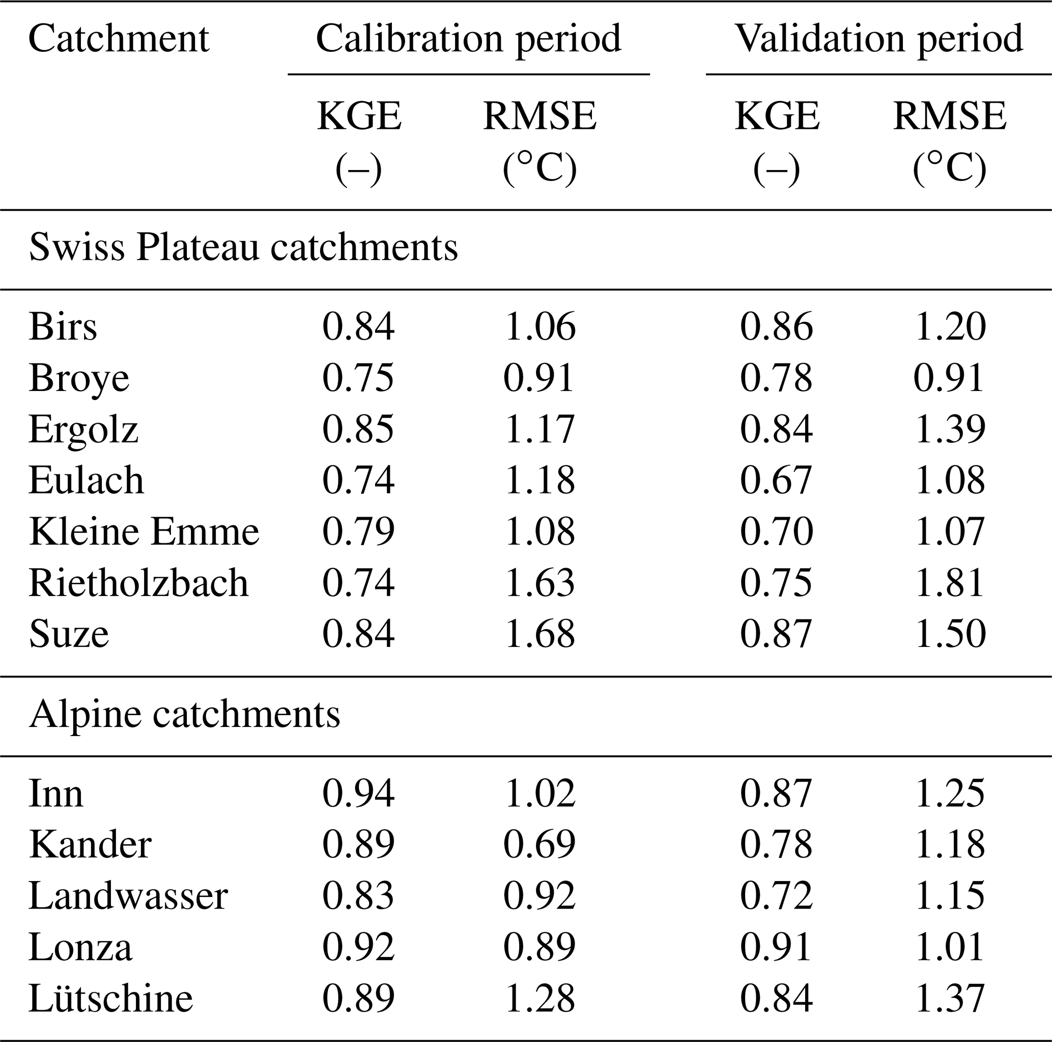
Figure 3 Daily mean water temperature observed (black) and simulated (red) over the calibration periods (left of dotted line) and over the validation period (right of dotted line) for four catchments: the Broye (Swiss Plateau), the Inn (Alpine), the Landwasser (Alpine), and the Suze (Swiss Plateau). These four catchments were chosen to represent the variation in the catchment type. Note that the extent of the y axes (daily mean water temperature range) is different for every panel. Other catchments are shown in Sect. S6.

4.1.1 Swiss Plateau catchments

Validation results of the Swiss Plateau catchments show that the KGE ranges between 0.67 and 0.87 and the RMSE between 0.91 and 1.81 ^∘C (Table 4). These values indicate a good performance compared to previous studies (e.g. Köplin et al., 2010; Råman Vinnå et al., 2018). The simulated validation time series for both discharge and water temperature lie in the range of the historical variability of the measurements (Figs. S6 to S19). The dynamics of high river temperature and discharge events as well as the annual cycles are well captured. There are no strong seasonal patterns of errors in river temperature (except for a slight underestimation in spring), and there is no correlation between errors in simulated discharge and river temperature (Figs. S6 to S19). However, there is an overestimation of discharge in winter but without an impact on the simulated water temperature.

The error in river temperature is slightly larger for the Suze catchment compared to the other Swiss Plateau catchments (see Table 4 and Fig. 3). We attribute this to the fact that this region is karstic, with enhanced water infiltration and resurgence to the surface, which impacts the water temperature. In addition, the gauging station is situated downstream of a cement factory, making anthropogenic influence on the stream temperature likely (see Michel et al., 2020). In the Eulach catchment, a large fraction of water (about 33 %) is directly lost to deeper groundwater via the calibrated water loss parameter. This is coherent with the ratio of precipitation and discharge observed in this catchment as described in Huggenberger and Epting (2011). A sizeable soil water loss is also modelled for the Birs. Again, this is not surprising, since both the Birs and Eulach catchments have been selected deliberately because of their river-fed ground-watershed in order to be used in the study of Epting et al. (2021). Finally, the longer run performed for the Broye catchment (2002–2018, Fig. S3) shows that river temperature in the extremely warm years 2003, 2015, and 2017 and the relatively cooler years 2007 and 2014 is well captured by the model.

4.1.2 Alpine catchments

Alpine3D and StreamFlow perform very well in terms of snow cover and discharge simulation in two of the five Alpine catchments. The annual discharge cycle is well reproduced for the Kander (Figs. S22, S23, and S31) and the Lütschine (Figs. S28, S29, and S33). The results are less good for the Inn (Figs. S26, S27, and S30) and the Lonza (Figs. S26 and S27); this is visible from the discharge plots, even though it is not necessarily reflected in the KGE values. For the Landwasser (Figs. S24, S25, and S32), the melt season starts too early, as shown by the negative correlation between discharge and river temperature errors in spring and summer. These issues highlight the difficulty of accurately reproducing snowmelt- and glacier-melt-induced runoff dynamics in Alpine environments even when using a very sophisticated snow model. A possible explanation is the scarcity of meteorological measurements in Alpine regions, which according to Magnusson et al. (2011) and Schlögl et al. (2016) decreases the performance of models.

Regarding water temperature, lower model performance is obtained for Alpine catchments in summer compared to Swiss Plateau catchments. Sudden water temperature peaks of up to +4 ^∘C above the corresponding measurements are occasionally simulated in summer, leading to an error of up to +2 ^∘C in the summer seasonal mean (Fig. 3).

Another illustration of overestimated summer water temperatures is the summer of 2003. Michel et al. (2020) used historical measurements to show that large amounts of snowmelt and glacier melt contribute to mitigating increased river temperature during hot summers. In their analysis, Alpine catchments in Switzerland were not affected by the extremely warm summer of 2003. In the present study, the model overestimates the temperature anomaly for the year 2003 in the high-Alpine Lonza catchment, while it produces correct results for the lowland Broye catchment (Fig. S3). Ample discussion on this issue and its consequences is presented in Sect. 5.1.

4.2 Climate change simulations

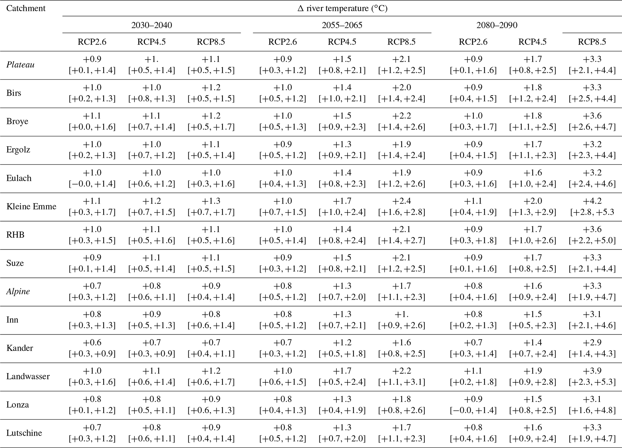
Simulation results are shown in terms of changes (delta) compared to the reference period 1990–2000. Absolute change is used for water, soil, and air temperature and relative change for the other variables. Detailed plots for each catchment are included in Sect. S10, Figs. S60 to S97. The results for annual mean river temperature for all the catchments are summarized in Table 5. Annual and seasonal values for all catchments are presented in Tables S9 to S12. Boxplots presented in this section are constructed from all CC scenarios and all individual years, so the range shows the model uncertainty, the natural inter-annual variability, and the catchment's variability when multiple catchments are combined.

Table 5 Change in annual mean river temperature for all three periods and three RCPs compared to the reference period 1990–2000. The median value of all years and scenarios is indicated together with the range of the values.

Before simulating the future discharge and river temperature, the performance of the models when forced with CC scenarios over the historical period was assessed. Section S8 shows that forcing the models with CC scenarios leads to small overestimation or underestimation of the total discharge in Alpine catchments. This is expected since the used CC scenarios show lower performance for precipitation in Alpine areas compared to Swiss Plateau areas (Warscher et al., 2019). Overall, it is confirmed that the output of Alpine3D and StreamFlow, when forced with CC scenarios over a historical time period, is consistent with the output obtained when forcing the models with measured meteorological inputs.

4.2.1 Swiss Plateau catchments

The model results from CC simulations over the Swiss Plateau catchments are similar among all considered catchments. The similarities in river warming between catchments show that catchment size does not play a noticeable role for the warming rate, as already observed for past periods (Michel et al., 2020).

Figure 4 shows the combined results for all considered Swiss Plateau catchments. For short-term projections, i.e. the period 2030–2040, the mean trend of averaged annual river temperature for the Swiss Plateau catchments is $+\mathrm{0.27}\pm \mathrm{0.03}$ ^∘C per decade (combining all three RCPs, the uncertainty indicated is the standard deviation), which is in line with the $+\mathrm{0.33}\pm \mathrm{0.03}$ ^∘C per decade observed over the whole of Switzerland for the period 1979–2018 (Michel et al., 2020). No significant annual discharge trends are modelled for this period.

Figure 4 Changes in river temperature (ΔT), air temperature (ΔTA), discharge (ΔQ), and precipitation (ΔPSUM), from left to right column, over the periods 2030–2040, 2055–2065, and 2080–2090 compared to the reference period 1990–2000 for the Swiss Plateau catchments and for the three RCPs. The first row shows the annual changes, the second row the winter seasonal changes, and the last row the summer seasonal changes.

Over the same period, the mean air temperature trend over Swiss Plateau catchments is 0.33±0.02 ^∘C per decade, corresponding to a ratio between river and air temperature trends of 0.8 for this period, which compares very well to the ratio obtained from historical observations (Michel et al., 2021b) and in the studies of Null et al. (2013) and Leach and Moore (2019). This result underlines the ability of the model chain to correctly capture the observed changes in the contemporary period. The expected water temperature increase is consistently more pronounced in summer than in winter for all studied catchments, time periods, and CC change scenarios.

For the periods 2055–2065 and 2080–2090, some differences between the RCP emission scenarios appear. For RCP2.6, no relevant additional changes are expected beyond 2030–2040. For RCP4.5, the situation between 2055–2065 and 2080–2090 remains similar, while for RCP8.5 there is an acceleration of changes in discharge and temperature. By the end of the century, the median annual river temperature increase reaches +3.5 ^∘C for RCP8.5. For some specific summers and CC scenarios, the warming can reach up to +6.5 ^∘C (Table S9). These results are in line with recent predictions of Swiss lake surface water temperature over the 21st century (Råman Vinnå et al., 2021). They are also comparable to results in the literature for other regions of the world with a comparable climate regime and using similar climate change scenarios and time periods. For example, Piotrowski et al. (2021) obtain an annual warming of +2 to +3 ^∘C for the period 2070–2100 for RCP8.5 in lowland catchments situated in the United States and in Poland using statistical and machine learning models. Similarly, a large-scale study by van Vliet et al. (2013) predicted a warming of +3 ^∘C by the end of the century for rivers in central Europe using the former SRES A2 scenarios (which predict a warming slightly lower than RCP8.5).

Changes in annual discharge patterns, linked to precipitation changes, appear with RCP4.5 and RCP8.5 in the periods 2055–2065 and 2080–2090 (more marked for RCP8.5 and for the latter period). An increase in winter discharge and a decrease in summer discharge are simulated with no significant change at the annual scale, except for RCP8.5 by the end of the century due to enhanced evapotranspiration (ET). Simulated changes in ET for four catchments are shown in Fig. S96, indicating a median increase in ET of about +15 % by the end of the century in the summer season combined with a deficit of precipitation of −13 % for the emission scenario RCP8.5. A special case is the Eulach catchment, which is much more urbanized compared to the other studied catchments, explaining the lower change in ET observed there. The changes in ET are similar for the RCP4.5 and RCP8.5 scenarios and only about 1.5 times larger than the one expected with the RCP2.6 scenarios, showing that ET will be limited mainly by water availability and that potential additional water during wetter summers will have a very high potential to evaporate. This is also seen from the large variability in ET for the RCP8.5 scenarios.

4.2.2 Alpine catchments

At the annual scale, the simulated water temperature increase in Alpine catchments is close to that observed across the Swiss Plateau (see Table 5) despite a slightly higher air temperature increase (see Figs. 4 and 5). The warming is more limited for the early periods in Alpine environments but reaches the same level as in the Swiss Plateau catchments towards the end of the century. This slower warming in Alpine catchments compared to the Swiss Plateau catchments in early periods of the 21st century is coherent with current trends observed in Switzerland (Michel et al., 2020). At the seasonal timescale, the change in river temperature is different between Swiss Plateau and Alpine catchments. In the Swiss Plateau catchments (Fig. 4), the warming is slightly higher in summer than in winter, with the spring and autumn seasons in between. In Alpine catchments (Fig. 5), the warming is rather limited in winter and spring but 2 to 3 times higher during summer and autumn.

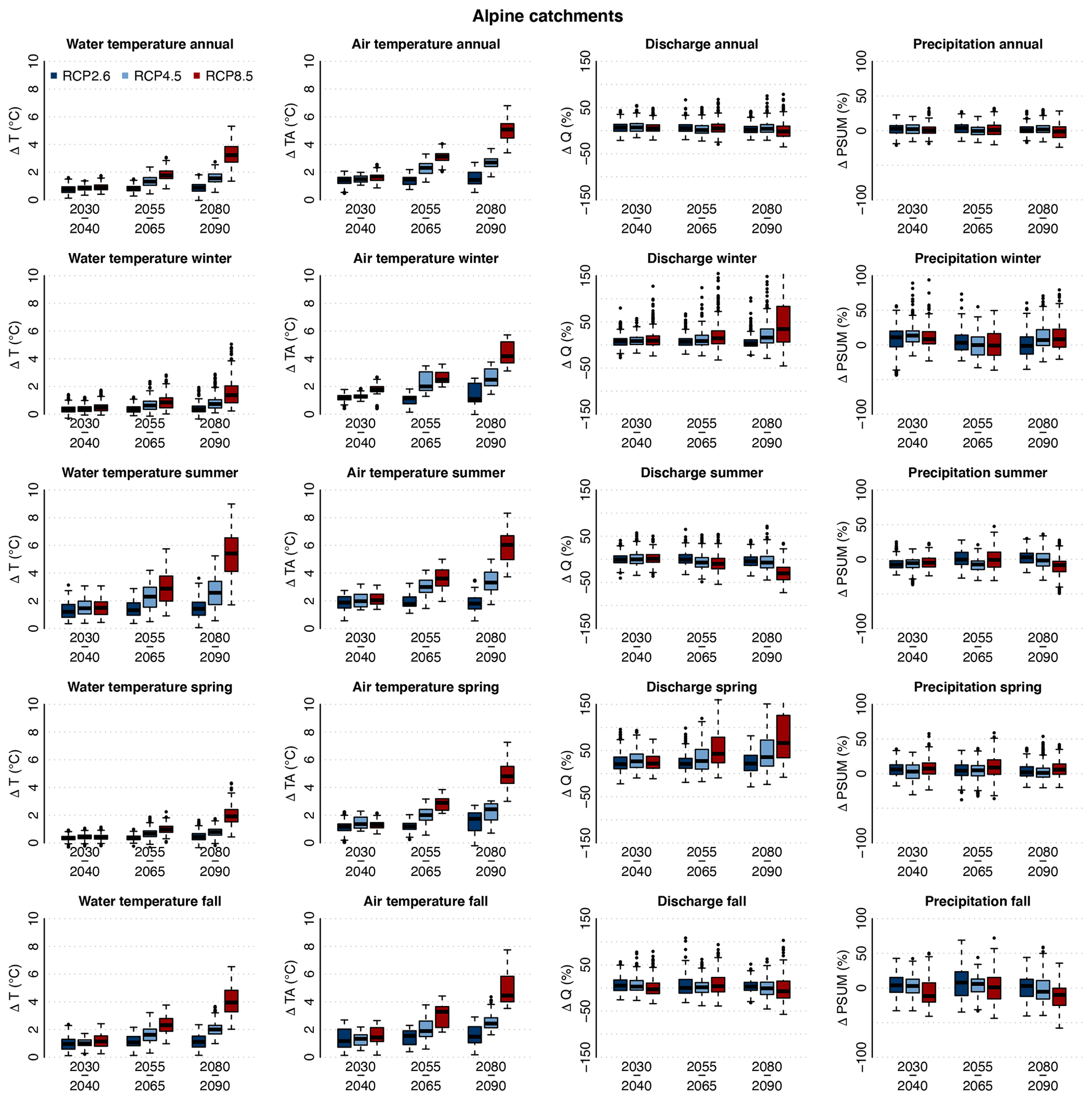
Figure 5 Changes in river temperature (ΔT), air temperature (ΔTA), discharge (ΔQ), and precipitation (ΔPSUM), from left to right column, over the periods 2030–2040, 2055–2065, and 2080–2090 and for the three RCPs compared to the reference period 1990–2000, averaged over all considered Alpine catchments. Row 1 shows the annual change, row 2 the winter seasonal change, row 3 the summer seasonal change, row 4 the spring seasonal change, and row 5 the autumn seasonal change.

To expand the analysis to other quantities simulated by Alpine3D, Fig. 6 shows the simulated evolution of snow and ice water equivalent, of solid precipitation, and of soil surface temperature on a yearly and seasonal basis for all considered Alpine catchments combined (for individual catchments, see Figs. S72 to S76). The annual discharge and temperature cycles for the four time periods and the three RCPs are shown for the Inn catchment in Fig. 7 (see also Figs. S77 to S80 for the other Alpine catchments). Finally, maps of snow and glacier covers for the five Alpine catchments, the periods 1990–2000 and 2080–2090, RCP2.6 and RCP8.5, and for the months of February, May, and December are shown in Figs. S81 to S95.

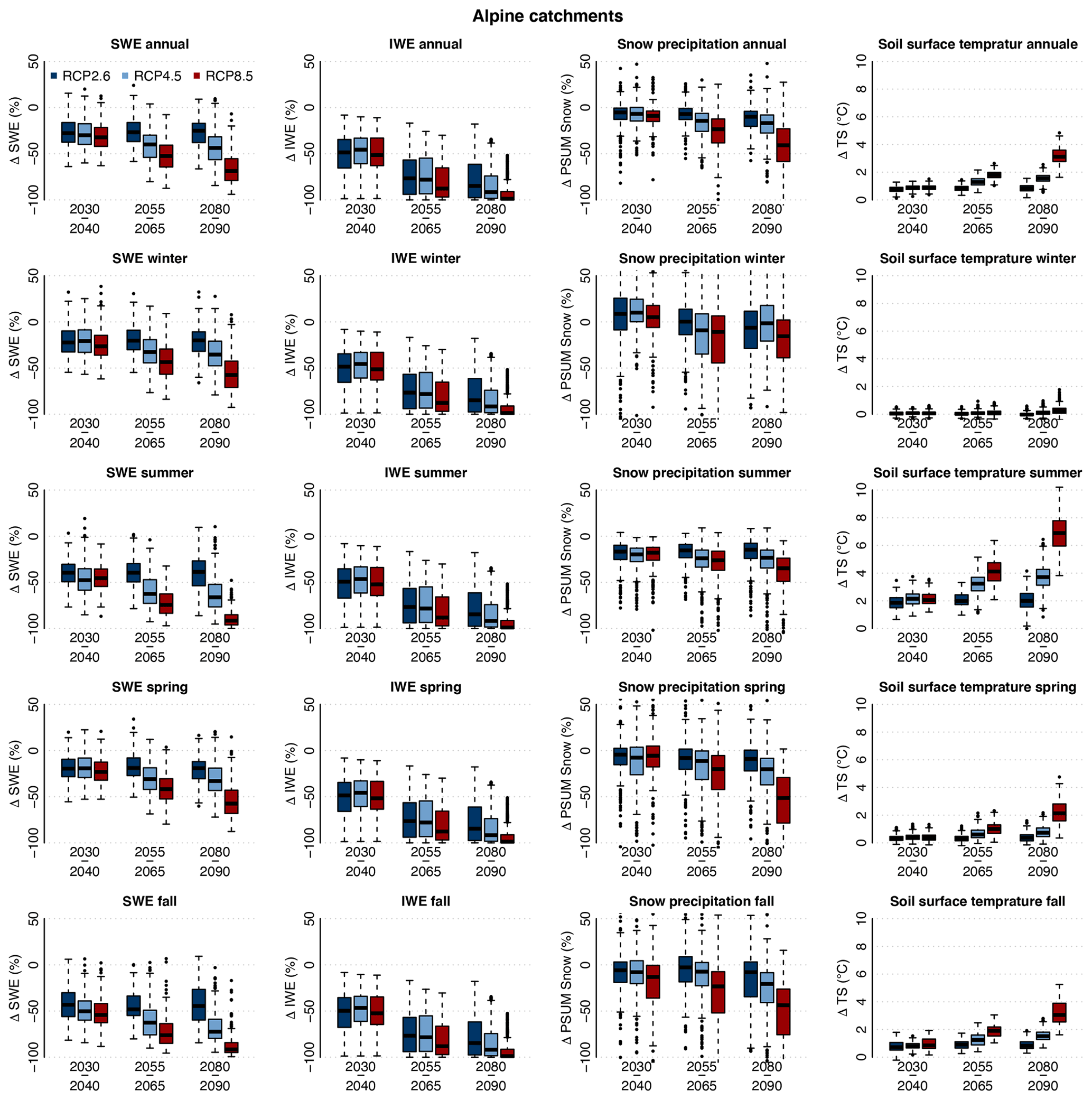
Figure 6 Changes in snow water equivalent in the catchments (ΔSWE), in ice water equivalent (mass of glacier ice and snow in glacier pixels) in the catchments (ΔIWE), in solid precipitation (ΔPSUM snow), and in soil surface temperature (ΔTS), from left to right column, over the periods 2030–2040, 2055–2065, and 2080–2090 and for the three RCP scenarios compared to the reference period 1990–2000, averaged over all considered Alpine catchments. Row 1 shows the annual change, row 2 the winter seasonal change, row 3 the summer seasonal change, row 4 the spring seasonal change, and row 5 the autumn seasonal change.

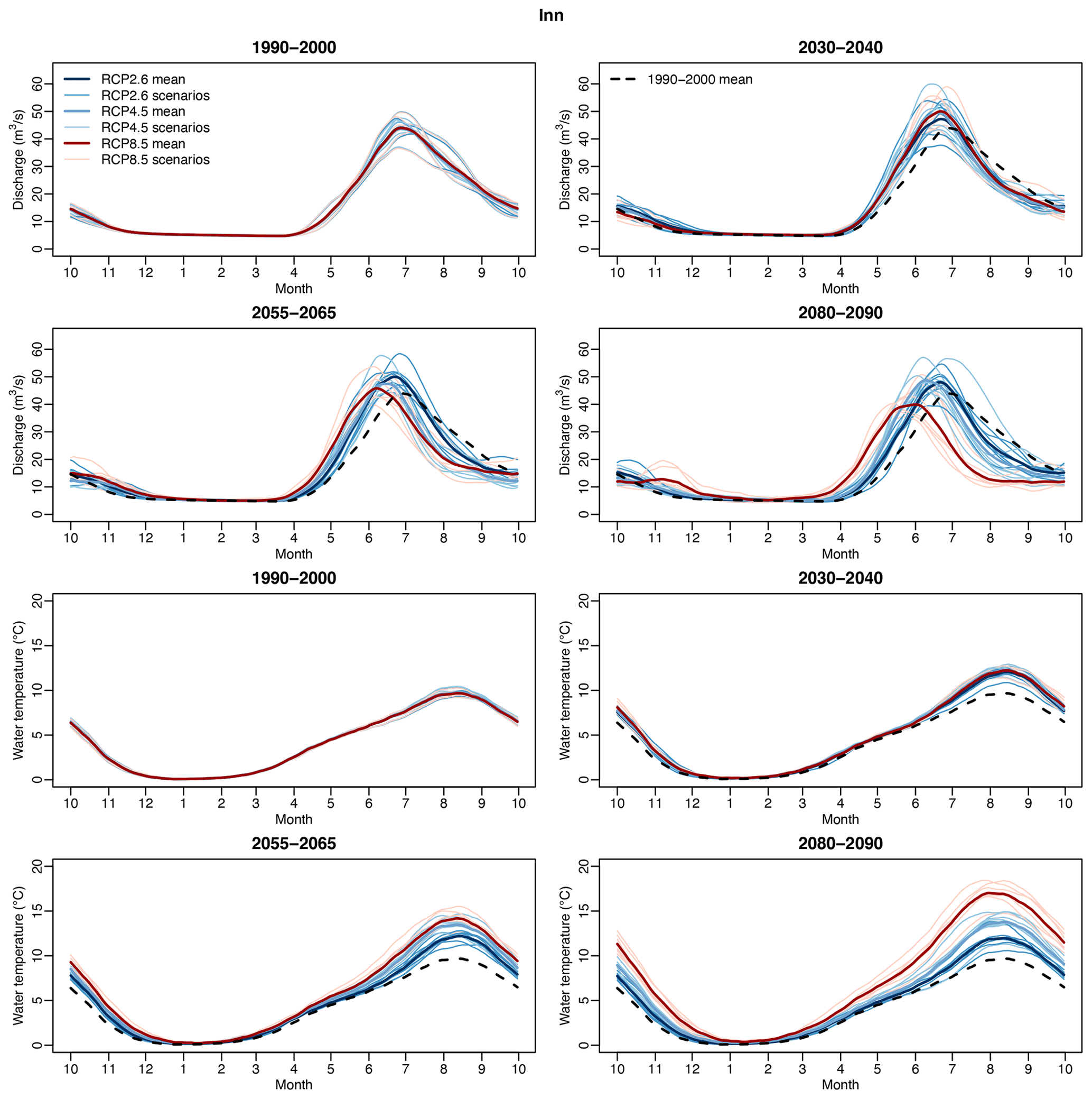
Figure 7 Annual cycle of discharge (top panels) and river temperature (bottom panels) of the Inn catchment. The cycles are obtained by computing the average for each day of the year and by applying a circular moving average of 30 d. Dark lines show the mean for each RCP over each period, and light lines show individual scenarios. Black dashed lines indicate the mean over the reference period 1990–2000 (only shown in subsequent periods to ease comparison).

During the winter season (Fig. 5), despite an air temperature increase similar to that projected for the Swiss Plateau, the river temperature increase is very limited, only reaching a median value of +1.4 ^∘C at the end of the century with RCP8.5 scenarios. This reduced winter warming in Alpine catchments is consistent with observations from the past decades (Michel et al., 2020). At the same time, an increase in discharge between +9 % in 2030–2040 (for the three RCP scenarios) and up to +35 % for RCP8.5 at the end of the century is expected. In the long term, no significant difference in winter precipitation is expected. The combination of the lower fraction of solid precipitation (i.e. more rain) and the enhanced snowmelt explains the increase in winter discharge.

The most important limiting factor for the Alpine river temperature rise in winter (even with a mean air temperature rise of up to +4.2 ^∘C for RCP8.5 at the end of the century compared to the reference period) is that the air temperature mostly remains below freezing at higher elevations, especially during the night. In these periods, the river temperature stays above the air temperature and does not experience any warming. In addition, for near-future periods or low-emission scenarios, the snow cover often prevents an increase in soil temperature in winter (Fig. 6).

During the spring season, earlier snowmelt occurs (Fig. 6), which becomes even more pronounced towards the end of the century and for RCP8.5 (the melt contribution to runoff will increase up to 20 %). In addition, a significant reduction of solid precipitation is expected in future spring seasons. These effects combined lead to a considerable increase in discharge and a shift of the peak runoff towards earlier times in the year. Even for the low- and moderate-emission scenarios RCP2.6 and RCP4.5, this shift is clearly visible at the end of the century. For RCP8.5, we observe a flatter peak occurring almost 2 months earlier than during the reference period (see Figs. 7 and S77 to S80). These results are consistent with findings of Muelchi et al. (2021a) concerning the evolution of discharge. Despite this increase in spring discharge, the river warming is slightly more marked in spring than in winter for the periods 2055–2065 and 2080–2090. As discussed in Sect. 5.1, the advection of cold water from snowmelt is not captured in the used model chain. Accordingly, the river temperature warming might be overestimated in spring since the predicted enhanced melting might inject considerable amounts of cold water into the stream network.

The summer season shows distinctively different changes in river temperature patterns and intensity between RCPs and time periods. For the near future (2030–2040), the expected river temperature increase remains below the air temperature increase, alike for the Swiss Plateau catchments. Advancing in time, and looking especially at RCP8.5 scenarios, the river warming catches up with the air temperature rise leading to a median river warming of +5.4 ^∘C (+5.9 ^∘C for the air temperature, Tables S9 and S10). However, since overestimation was observed during the model validation for summer over the Alpine catchments, these results need to be carefully interpreted and discussed (see Sect. 5.1).

During autumn, a discharge reduction occurs at the beginning of the season, caused by the shift of annual peak discharge to earlier in spring and summer, followed by a discharge increase later in the season due to an increased fraction of liquid precipitation and rapid melting of occasional snowfall. Such autumn melt events contribute to cooling the soil; accordingly, the water temperature increase is similar to the one predicted over the Swiss Plateau.

5 Discussion

5.1 Model chain performance

For the Swiss Plateau catchments, the errors in river temperature (RMSE) obtained during the calibration and validation periods are far below the CC signal for RCP4.5 and RCP8.5, which underlines the robustness of the simulated trends. The results obtained are coherent with past and current observations in Switzerland and in central Europe (Moatar and Gailhard, 2006; Webb and Nobilis, 2007; Arora et al., 2016; Michel et al., 2020) and are in agreement with other results in the literature, both in terms of predicted changes in discharge and water temperature and in terms of processes and CC sensitivity (Null et al., 2013; Ficklin et al., 2014; Du et al., 2019; Leach and Moore, 2019; Wondzell et al., 2019; Muelchi et al., 2021a; Piotrowski et al., 2021). The studied catchments can be assumed to be representative of undisturbed Swiss catchments in general (Michel et al., 2020).

For Alpine catchments, the calibration results for discharge and water temperature show a low model error in winter, spring, and autumn. Over these seasons, results are coherent with observed trends. Summer discharge and snow depletion in the melt season are not perfectly captured in all catchments, but results are coherent with the literature (Brunner et al., 2019a; Muelchi et al., 2021a). During summer, simulated river temperatures show instances of sudden overestimation in four out of the five studied Alpine catchments. These overestimations do not appear during all summers, and there is no temporal coincidence between the instances of temperature overestimation and low discharge conditions. Furthermore, only two of the rivers concerned with this overestimation problem (the Inn and the Landwasser) show a correlation between river temperature and discharge errors (Figs. S21, S23, S25, S27, and S29), suggesting that the underestimation of summer discharge cannot explain the overestimation of river temperature.

Section S9 extensively discusses the influence of solar radiation and other energy fluxes on temperature simulation errors in Alpine catchments. In summary, it can be stated that the approximation of topographic shading due to the spatial resolution of Alpine3D and the underestimation of riparian vegetation shading can slightly contribute to the overestimation of summer river temperature but does not explain the magnitude and behaviour of the observed errors. The analysis rather suggests that the small upstream reaches are overly sensitive to variations in the forcing, causing too high a temperature in the upper part of the catchment, which then becomes advected downstream.

The most probable hypothesis explaining this over-sensitivity is that some mechanisms are not explicitly captured in the model. All the water draining from the snowpack is assumed to infiltrate the soil at the pixel scale in Alpine3D, while the runoff at the bottom of the soil column is collected in StreamFlow at the sub-catchment scale after a transfer through the two linear reservoirs emulating fast and delayed lateral sub-surface runoff. The water leaving these two reservoirs inherits the temperature determined by the sub-catchment temperature scheme in use. The fact that the model performs well in Swiss Plateau catchments regardless of catchment size and local topography suggests that the problem for Alpine catchments is related to processes that are only at play at high elevations. The following processes are not explicitly simulated in StreamFlow (in any of the implemented schemes for infiltrating soil water temperature) and can all contribute to the mentioned temperature overestimation during summer: (i) cold water advection from remaining, hydrologically well-connected snow patches (connected via surface and sub-surface flow; see Yan et al., 2021), (ii) cold water advection from local groundwater systems (see Thornton et al., 2021), and (iii) cold water advection from melting glacier ice (if present; see Du et al., 2021).

The chosen HSPF approach for sub-catchment infiltrating water temperature is shown to generally perform well in comparison to other approaches (see Sect. 3.4 and Leach and Moore, 2015), but it is exclusively based on air temperature and cannot explicitly capture any of the three processes mentioned above (note that the other two available approaches lead to even more problematic results during the summer season). This has only little impact on the simulated river temperatures in spring, when the air temperature is still relatively low. In summer, however, ignoring these cooling mechanisms can explain the exaggerated sensitivity of small upstream reaches. Figure S59 shows the infiltrating water temperature simulated by the HSPF scheme over the Landwasser catchment and its correlation with the simulated overestimation in summer, confirming that the HSPF scheme might be the cause of the overestimation. Our results suggest that this simple approach is not suited for complex Alpine terrain and that a different and probably more complex method should be developed.

The cooling effects from snowmelt and glacier melt, which are missing in the model, can be expected to become less important in the future because of the general glacier retreat and the increase in the average winter snow line. In addition, the Alpine3D simulations performed here show that, in spring, the median of the SWE reduction under RCP8.5 by the end of the century is about −60 %, meaning that the available snow to be melted in summer is reduced by the same amount.

In fact, the lack of proper cold water input parameterization can even be expected to actually result in an underestimation of the computed river warming in Alpine catchments. This would arise if the CC signal is computed with respect to a past period with summer temperature overestimation caused by missing cold water advection and if this effect disappears in the future (Du et al., 2021). However, we cannot conclusively attribute the overestimation to snowmelt and glacier melt not being captured, and other factors might be at play here.

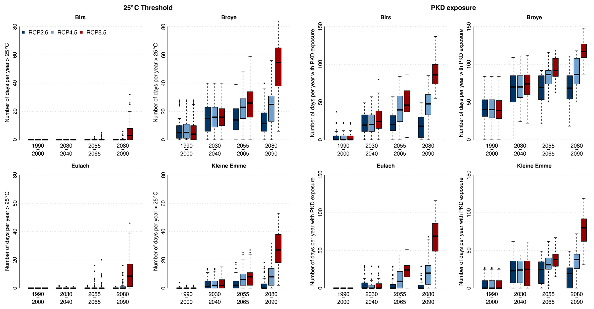
Figure 8 Left panels: number of days per year when the river temperature is above the threshold of 25 ^∘C, for each year in each time period and for each scenario, for four Swiss Plateau catchments. Right: number of days per year when salmonid populations are exposed to PKD, based on the metric presented in Michel et al. (2020), for each year in each time period and for each scenario, for four Swiss Plateau catchments. These four catchments were chosen to represent the variation in the Swiss Plateau catchment type.

Consequently, the results obtained for summer warming in Alpine rivers should be interpreted with caution. The main result of this part of the study is to show the need for more complex models to reliably simulate all the water flowpaths and thermal interactions in Alpine terrain.

Despite the limitations for the summer season in Alpine catchments, the simulated seasonal warming pattern, particularly pronounced in summer, is in agreement with results of Du et al. (2019) for the partially glaciated Athabasca catchment in Canada, of Piotrowski et al. (2021) for the mountainous cedar catchment in Poland, and of Ficklin et al. (2014) over the Columbia River basin in the western US and Canada. For the period 2081–2100 and RCP8.5, Ficklin et al. (2014) obtained river temperature warming comparable to or higher than that of the air temperature for the upper part of the catchment, similar to our results for Alpine catchments.

In summary, we show the high skill of the used physics-based model chain to reproduce discharge and water temperature in the Swiss Plateau catchments. For the Alpine catchments, good results are obtained in all seasons except for summer, and mechanisms explaining this lower performance are provided.

5.2 Climate change impact

The expected increase in river temperature will have a large impact on both natural and societal systems. To evaluate this future impact, we use two metrics introduced by Michel et al. (2020): (i) the number of days per year when the daily maximum river temperature is above 25 ^∘C (this is a legal threshold in Switzerland for unrestricted water usage, e.g. for industrial cooling) and (ii) a metric indicating the number of days per year when salmonid fish are exposed to PKD. The latter metric is based on the model of Carraro et al. (2016), counting the number of days per year for which the minimum daily temperature exceeds 15 ^∘C for at least 28 consecutive days. Values for these two indicators are shown for four catchments in Fig. 8. Note that these two metrics are meaningful only for Swiss Plateau catchments.

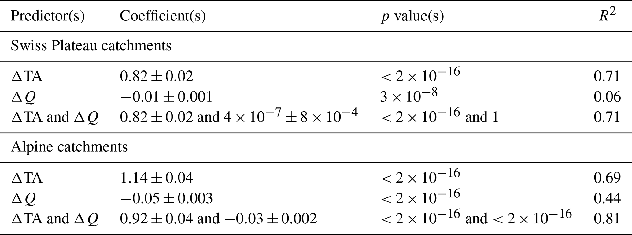
Table 6 Summary of the linear models for changes in river temperature (ΔT) using changes in air temperature (ΔTA), water discharge (ΔQ), or both as predictors. Changes in the period 2080–2090 compared to the reference period 1990–2000 are used for RCP8.5. The table shows the coefficients, the p values associated with each predictor, and the adjusted R² (discounting the effect of additional explanatory variables) of each model. The linear models are applied separately for the Swiss Plateau catchments (top) and the Alpine catchments (bottom).

The metrics values obtained over the historical period match well the corresponding values obtained from measurements (Michel et al., 2020), underlining again the robustness of the results obtained when the models are forced with CC scenarios. For each of the four catchments shown in Fig. 8, both indicators grow over time and with increased greenhouse gas emissions. Catchments such as the Birs and the Eulach, which are currently less prone to high river temperatures, will reach and exceed both the legal threshold of 25 ^∘C and the PKD critical value more frequently in the future. By the middle of the century, river temperature conditions during summer will be favourable for the spread of PKD in all seven investigated catchments (for all RCPs), with possibly devastating impacts on the salmonid fish population. For catchments with relatively warm river water under current conditions, such as the Broye and the Kleine Emme, the legal limit of 25 ^∘C will be reached almost every year already by 2030–2040 regardless of the emission scenario. By the end of the century, and with high-emission scenarios, the river temperature will be above this threshold for around 2 months per year in these two catchments. This will prompt either stoppage of regular water usage for industry and cooling in such catchments or a necessary adaptation of current regulation and legislation at the risk of further enhancing the impacts and increasing the stress and pressure on these ecological systems.

In Alpine catchments, the large decrease in summer snow cover and the shrinking of glaciers (Huss and Hock, 2018; Compagno et al., 2021) lead to a drastic warming of the soil surface owing to lower surface albedo and the absence of a thermally insulating layer (Fig. 6). In 2030–2040 (all scenarios) and during the second part of the 21st century under RCP2.6, this soil warming remains limited, with an increase lower than that of the air temperature. However, for RCP4.5 and RCP8.5 and periods further ahead, these changes in land cover cause a substantial soil temperature increase, which can exceed the warming of the air temperature. Such an increase in soil temperature is not simulated for the lowland catchments (Fig. S97). In addition, Alpine catchments will experience a sharp decrease in discharge during the second half of the summer (see Fig. 7), which might exacerbate the sensitivity of the rivers to energy input and contribute to higher temperatures in the summer season. Therefore, despite the uncertainty linked to the simulated summer river temperatures, our results provide strong evidence of a more pronounced warming during summer in Alpine rivers compared to lowland rivers (which is also consistent with the literature).

Discharge reduction is mentioned in the previous paragraph as a factor of enhanced water warming. From simple thermodynamics, we can expect reduced discharge to have a direct impact on river temperature. However, historical data do not exhibit a strong correlation between changes in discharge and changes in river temperature during summer, except during unusually warm and dry summers, when low discharge exacerbates the warming (Michel et al., 2020). In Alpine catchments, the summer mean water temperature has been shown to have a low inter-annual variability, even during dry and warm summers (Michel et al., 2020).

To investigate the relationship between changes in river temperature and discharge during summer, we apply univariate and multivariate linear models to ΔT, taking ΔTA, ΔQ, or both as predictors. The models are applied separately for the Swiss Plateau and for the Alpine catchments for the summer season, for the period 2080–2090, and for RCP8.5 (Table 6 and Fig. S98). For the Swiss Plateau catchments, both ΔTA and ΔQ are identified as significant predictors when used separately (with an adjusted-R² of only 0.06 when using ΔQ), but when used together the significance of ΔQ disappears and the explanatory power of the model is not improved compared to using ΔTA alone. Thus, in the Swiss Plateau catchments, there is no strong correlation between changes in summer discharge and changes in river temperature. This is coherent with historical observations and with results by Wondzell et al. (2019), which show a much weaker impact of discharge change on water temperature compared to changes in air temperature for the upper Middle Fork John Day River, northeastern Oregon, USA.

In Alpine catchments, ΔQ remains significant in the multivariate model and increases the R² value from 0.69 (when using only ΔTA) to 0.81. In addition, using ΔQ alone allows us to explain almost half of the variability in ΔT. Due to the problem of overestimated summer river temperatures in Alpine catchments, we have low confidence in this specific result and cannot draw a convincing conclusion on possible differences between lowland and Alpine catchments concerning the sensitivity of river temperature to discharge. Accurately quantifying this sensitivity in Alpine regions in a changing climate, with the expected decrease in snow and glacier cover, would be of great interest in further studies.

5.3 Current limitations and future model development

Besides the problem of simulating summer river temperature in Alpine catchments, there are a few other shortcomings in the models used. Riparian vegetation is not completely accounted for in the model chain Alpine3D–StreamFlow, while it is shown to have a strong local effect on river temperature (see among others Kalny et al., 2017; Trimmel et al., 2018; Dugdale et al., 2018; Wondzell et al., 2019). The integration of riparian vegetation would be a necessary addition in such models to assess its effectiveness as a mitigation strategy. Also, no dynamic interaction with the water table is represented in the model. Interaction with groundwater might be a significant factor for water temperature in some catchments (Qiu et al., 2019; Johnson et al., 2020; O'Sullivan et al., 2020). Further model improvement to better represent the interplay of water infiltration in soil, cold water advection, and groundwater dynamics might be key elements in future CC impact assessments of water temperature because this might come in parallel with recently developed methods for groundwater and irrigation water management (García-Gil et al., 2015). Such methods could even include specific thermodynamic water management, such as water infiltration during winter for river cooling during summer (Epting et al., 2013).

Further extensions are needed to account for anthropogenic influences like dams, pumping, deviations, intakes, or discharge, which influence the water temperature (Michel et al., 2020; Seyedhashemi et al., 2021) but are not considered in the model used, limiting the current study to mostly natural undisturbed catchments. In addition, Michel et al. (2020) showed with historical data that the presence of lakes along the watercourse changes the warming rate of rivers. This two-way interaction in river–lake–river systems also remains to be investigated in more detail in future studies, especially considering the expected shifts in lake mixing (Råman Vinnå et al., 2021) and in the Alpine flow regime.

Future extreme events are not covered here because the used models are not validated for extreme events and the forcing time series do not capture such events (Michel et al., 2021b). In central Europe, a clear link between summertime dry spells and heat waves has been found (Fischer et al., 2007b, a), and both are expected to increase in frequency and amplitude in the future (NCCS, 2018). As a consequence, it is likely that even more pronounced warming than predicted here will result during extremely warm and dry summers in the future.

Finally, only one model chain is used for the snow and hydrological simulations, while significant differences can be obtained across models in terms of discharge and water temperature simulation over climate change periods (Carletti et al., 2021; Piotrowski et al., 2021).

6 Conclusion

This work presents the first extensive study of climate change (CC) impact on river temperatures in Switzerland and, to the best of our knowledge, in Alpine areas. A chain of physics-based models is used with 21 CC scenarios, spanning three different emission pathways (RCP2.6, RCP4.5, and RCP8.5). The model chain is applied to two categories of catchments, namely the lowland Swiss Plateau catchments and the higher-elevation Alpine catchments, which exhibit different discharge and thermal regimes.

We demonstrate the ability of a physics-based model chain to reliably simulate the river temperature in a variety of catchments in Switzerland, with a notable exception for summer water temperature in Alpine catchments. We tested several aspects of the physics-based models, such as the impact of using different calibration periods, using a lumped approach versus a discretized approach for water routing or using a simple in-stream routing computation versus a more complex scheme. Higher-complexity routing and discretization schemes do not improve the quality of the simulations. Results show the critical importance of correctly computing the water temperature entering the stream network in Alpine catchments; the results furthermore underline that omitting processes, such as cold water advection originating from snowmelt and ice melt or local cold water storage, could lead to an overestimation of the river temperature during summer. In this sense, this study offers a broad and solid foundation for future development and application of physics-based hydrological models in the context of CC modelling. The study identifies a few flaws of the models and provides evidence for necessary improvements in these models.

The results of the climate change impact study show that a distinct warming of river water is expected for the 21st century in all the investigated regions. By the end of the century (2080–2090), the median annual river temperature increase in the studied catchments amounts to +0.9 ^∘C for RCP2.6 (with a range of 0.0–1.9 ^∘C) and to +3.3 ^∘C for RCP8.5 (1.4–5.3 ^∘C) compared to the reference period 1990–2000. A significant reduction in summer discharge is predicted for high-emission scenarios by the end of the century, with a median value of −27 % for the Swiss Plateau catchments and of −31 % for the Alpine catchments. At the seasonal timescale, the warming on the Swiss Plateau and in the Alpine regions exhibits different patterns. On the Swiss Plateau the summer warming only slightly exceeds the winter one (by about 20 %), and it is only weakly affected by changes in discharge. In the Alpine catchments, the warming is rather limited during the cold months. In summer, the identified model limitations regarding river temperature simulation lower our confidence in the exact value of the predicted warming. However, we show that sizeable decrease in snow and ice cover expected during summer will lead to a significant increase in soil temperature, which then will most likely lead to large further river warming. In addition, this study quantifies the expected reduction in cold water advection from melting glacier and snow, which is also expected to contribute to the summertime river warming in Alpine catchments.

Our results show that river systems in Switzerland (and likely all of the Alps and the adjacent regions) will undergo substantial changes in the near future in terms of both water temperature and water availability. Two metrics have been used to quantify future impacts of river warming on ecology and on industrial cooling water use. This highlights the urgent need for both adaptation and mitigation strategies. The current rapid advances in water temperature modelling should thus cross the boundaries of purely scientific applications and be made available to a broader public for operational use in water temperature forecast and warning systems. Future development of monitoring systems will also be of great importance for improving the understanding of water temperature processes and their representation in models.