the Creative Commons Attribution 4.0 License.
the Creative Commons Attribution 4.0 License.
 | 19 Feb 2021
Uncertainty of simulated groundwater recharge at different global warming levels: a global-scale multi-model ensemble study
Robert Reinecke
Hannes Müller Schmied
Tim Trautmann
Lauren Seaby Andersen
Peter Burek
Martina Flörke
Simon N. Gosling
Manolis Grillakis
Naota Hanasaki
Aristeidis Koutroulis
Yadu Pokhrel
Wim Thiery
Yoshihide Wada
Satoh Yusuke
Petra Döll
Billions of people rely on groundwater as being an accessible source of drinking water and for irrigation, especially in times of drought. Its importance will likely increase with a changing climate. It is still unclear, however, how climate change will impact groundwater systems globally and, thus, the availability of this vital resource. Groundwater recharge is an important indicator for groundwater availability, but it is a water flux that is difficult to estimate as uncertainties in the water balance accumulate, leading to possibly large errors in particular in dry regions. This study investigates uncertainties in groundwater recharge projections using a multi-model ensemble of eight global hydrological models (GHMs) that are driven by the bias-adjusted output of four global circulation models (GCMs). Pre-industrial and current groundwater recharge values are compared with recharge for different global warming (GW) levels as a result of three representative concentration pathways (RCPs). Results suggest that projected changes strongly vary among the different GHM–GCM combinations, and statistically significant changes are only computed for a few regions of the world. Statistically significant GWR increases are projected for northern Europe and some parts of the Arctic, East Africa, and India. Statistically significant decreases are simulated in southern Chile, parts of Brazil, central USA, the Mediterranean, and southeastern China. In some regions, reversals of groundwater recharge trends can be observed with global warming. Because most GHMs do not simulate the impact of changing atmospheric CO2 and climate on vegetation and, thus, evapotranspiration, we investigate how estimated changes in GWR are affected by the inclusion of these processes. In some regions, inclusion leads to differences in groundwater recharge changes of up to 100 mm per year. Most GHMs with active vegetation simulate less severe decreases in groundwater recharge than GHMs without active vegetation and, in some regions, even increases instead of decreases are simulated. However, in regions where GCMs predict decreases in precipitation and where groundwater availability is the most important, model agreement among GHMs with active vegetation is the lowest. Overall, large uncertainties in the model outcomes suggest that additional research on simulating groundwater processes in GHMs is necessary.
- Article
(7324 KB) - Full-text XML
-
Supplement
(34839 KB) - BibTeX
- EndNote


The critical role of groundwater as an accessible source for irrigation and of drinking water, in particular during dry periods, droughts, and floods, will intensify with climate change because increased precipitation variability is expected to decrease the reliability of surface water supply (Taylor et al., 2013; Döll et al., 2018; Kundzewicz and Döll, 2009). While demand for groundwater is likely to increase in the future, groundwater abstractions have already led to depleted aquifers in many regions around the globe (Thomas and Famiglietti, 2019; Cuthbert et al., 2019a; Wada et al., 2012; Konikow and Kendy, 2005; Döll et al., 2014b). They have also resulted in the reduction in groundwater discharge to rivers, with negative impacts on water availability for humans and freshwater biota, in particular during low-flow periods (Herbert and Döll, 2019). To what extent groundwater can serve to sustain ecosystem health and to support human adaptation to climate variability and change strongly depends on future groundwater availability, which is strongly affected by climate change (Kundzewicz and Döll, 2009; Döll, 2009; Taylor et al., 2013; Cuthbert et al., 2019b).
Groundwater recharge (GWR) is a central indicator of potential groundwater availability (Herbert and Döll, 2019). GWR is the vertical water flux to the groundwater from the soil (diffuse GWR) and from surface water bodies (point or focused recharge; Small, 2005). It is a function of the local climate, topography, soil, land cover, land use (urbanization, woodland establishment, crop rotation, and irrigation practices), atmospheric CO2 concentrations, and geology (Small, 2005). Changes in GWR alter groundwater levels and their temporal patterns, which affect vital ecosystem services (Kløve et al., 2014). Knowledge of the dynamics and process interactions determining GWR is a fundamental prerequisite for assessing groundwater quality and quantity under climate change (Green et al., 2011). The simulation of GWR is possibly one of the most challenging components of the water budget as it accumulates the uncertainties of all other components of the budget. Especially in semiarid regions, uncertainties in precipitation and evapotranspiration (Wartenburger et al., 2018) lead to considerable uncertainty in recharge. An additional factor in estimating groundwater recharge is the simulation of the groundwater table and, thus, capillary rise and focused recharge. This has not been achieved yet in GHMs; however, recently, global hydrological models (GHMs) started integrating gradient-based groundwater models to better estimate the flows between surface water and groundwater and the impact of humans and the changing climate on the groundwater system (de Graaf et al., 2019; Reinecke et al., 2019). Neglecting capillary rise may lead to an overestimation of the decreases and increases in GWR due to a changing climate.
Assessing the response of GWR to climate change is difficult even at the local scale, with one of the reasons being that groundwater recharge, different from streamflow, is rarely measured, and long time series of groundwater recharge are not available (Earman and Dettinger, 2011). In local groundwater modeling, groundwater recharge is often determined by calibration using hydraulic head observation, while integrated modeling relies on the partitioning of precipitation into evapotranspiration, storage change, and runoff (GWR plus surface and subsurface runoff). Moreover, projections of GWR often neglect the impact of changing climate and higher CO2 levels on plants and, thus, evapotranspiration and GWR (Taylor et al., 2013). With higher CO2 levels, terrestrial plants open their stomata less, which reduces evapotranspiration and increases runoff (physiological effect), while they might grow better, increasing evapotranspiration (structural effect; Gerten et al., 2014). Vegetation models that include these effects disagree about the balance of both effects (Gerten et al., 2014). However, based on a large ensemble of GCMs that include the impact of CO2 and changing climate on vegetation and evapotranspiration, rising CO2 can be expected to decrease transpiration and, thus, increase total runoff (Milly and Dunne, 2016). Therefore, GHMs that do not consider active vegetation may underestimate runoff, and, thus, GWR increases, or they may overestimate GWR decreases.
While there have been review articles on the relation between groundwater and climate change (Smerdon, 2017; Jing et al., 2020; Refsgaard et al., 2016), global-scale studies that quantify the impact of climate change on GWR are rare. They have evolved regarding the way climate scenarios are implemented and how many global climate models (GCMs) and GHMs are included in the study. While Döll (2009) could only use the delta change method to integrate information from two GCMs in the GHM WaterGAP (Alcamo et al., 2003; Müller Schmied et al., 2014), Portmann et al. (2013) could feed their simulations of future changes in GWR with WaterGAP directly by means of the bias-adjusted output with five GCMs. They found that changes in GWR increase with increasing greenhouse gas emissions. Acknowledging that not only GCMs but also GHMs contribute to the uncertain translation of emissions scenarios to changes in GWR (Moeck et al., 2016), the study of Döll et al. (2018) included two GHMs (WaterGAP and LPJmL – Lund Potsdam Jena managed Land; Rost et al., 2008; Schaphoff et al., 2013) driven by the bias-adjusted output of four GCMs. They evaluated relative changes in GWR with climate change, which can arguably serve as a better indicator of climate change hazard than absolute changes in GWR. On the other hand, the usage of relative change led to the result that change in GWR could not be reliably computed for 55 % of the global land area due to very small GWR for the reference period simulated by LPJmL (Döll et al., 2018). While the LPJmL model considered, differently to the WaterGAP model, the effect of rising CO2 on groundwater recharge, the impact of this on GWR projections were not analyzed in Döll et al. (2018). In general, studies investigating the difference between GHMs with and without dynamic vegetation are rare (Davie et al., 2013).
This study assesses the impact of climate change on GWR based on the output of a multi-model ensemble encompassing eight GHMs, each forced by the bias-adjusted output of four GCMs under three different representative concentration pathways (RCPs). The ensemble was generated in the framework of the Inter-Sectoral Impact Model Intercomparison Project (ISIMIP) using simulation protocol ISIMIP2b (Frieler et al., 2017). The ISIMIP global water sector incorporates global models, including water resources models, land surface models, and dynamic vegetation models, which can compute water flows and storages on the continents of the Earth; in this study, all three model types are referred to as GHMs. The ISIMIP2b ensemble has already been used in multiple climate change studies investigating, for example, flood risk (Willner et al., 2018; Thober et al., 2017; Alfieri et al., 2017), low flows in Europe (Marx et al., 2018), evapotranspiration (Wartenburger et al., 2018), runoff and snow in Europe (Donnelly et al., 2017), drought severity (Pokhrel et al., 2021), heat uptake by inland waters (Vanderkelen et al., 2020), and multi-sectoral impacts (Byers et al., 2018; Lange et al., 2020).
We analyze how GWR is projected to change globally and regionally for multiple global warming (GW) levels, determine the contributions from GHMs and GCMs to the variance of simulated changes, and discuss the implications for future assessments of global groundwater resources. Furthermore, we show the effect of including the physiological impacts of evolving CO2 on global estimates of GWR. To this end, the remainder of this paper is structured as follows. Section 2 provides an overview of the used GHMs and the methods for calculating changes in GWR per GW level and sources of uncertainty. The results in Sect. 3 show the significant changes in GWR per GW and the differences between GHMs and GCMs. We then compare the influence of GCMs, GHMs, and RCPs on the variance of simulated GWR, assess the differences in GWR due to including dynamic vegetation in GHMs, and compare the GHM simulations to interpolated measured GWR. The paper closes with a discussion of these findings (Sect. 4) and conclusions (Sect. 5).
2.1 Simulation of groundwater recharge
This study encompasses eight GHMs that differ in their representation of various hydrological processes. Four of these models are able to simulate the impact of evolving CO2 concentrations on vegetation: CLM 4.5, JULES-W1, LPJmL, and MATSIRO (Table 1). In the following, we use the term active vegetation for models that consider the physiological effect of changes in CO2 on vegetation and the term dynamic vegetation for the models that allow for changing vegetation regarding leaf area index (LAI) and/or vegetation type. A comprehensive overview of GHMs and their properties can be found in Sood and Smakhtin (2015). Detailed model descriptions and evaluations of the models can be found in the primary publications referred to in the subsections below and Telteu et al. (2021; for the model parameterization see Sect. 2.2). The definition of GWR and groundwater varies in between GHMs (discussed in Sect. 4). The analysis in this study is based on monthly GWR (variable qr in ISIMIP) in grid cells simulated by the eight GHMs taking part in the ISIMIP2b protocol (Frieler et al., 2017). Some GHMs contained small negative GWR values, for example, due to capillary rise; these values were set to zero in the analysis. We do not consider focused recharge in this study as no model has offered a reliable implementation of these processes until now. Also, none of the models simulate the depth of the groundwater table beneath the land surface, which does not allow us to correctly attribute delays in recharge due to water table depth.
Table 1Overview of which models are able to simulate the impact of evolving CO2 concentrations on vegetation and how it is implemented.

2.1.1 WaterGAP2
The WaterGAP2 model (Alcamo et al., 2003) computes human water use in five sectors and the resulting net abstractions from groundwater and surface water for all land areas of the globe, excluding Antarctica. These net abstractions are then taken from the respective water storages in the WaterGAP Global Hydrology Model (WGHM; Müller Schmied et al., 2014; Döll et al., 2003, 2012, 2014b). With daily time steps, WGHM simulates flows among the water storage compartments canopy, snow, soil, groundwater, lakes, human-made reservoirs, wetlands, and rivers. GWR in WaterGAP2 is calculated as being a fraction of runoff from land based on soil texture, relief, aquifer type, and the existence of permafrost or glaciers, taking into account a soil-texture-dependent maximum daily groundwater recharge rate (Döll and Fiedler, 2008). If a grid cell is defined as semiarid or arid and has a medium or coarse soil texture, GWR will only occur if daily precipitation exceeds a critical value (Döll and Fiedler, 2008); otherwise, the water runs off. Runoff from land that does not contribute to GWR is transferred to surface water bodies as fast surface runoff. WaterGAP further computes focused recharge beneath surface water bodies in semiarid and arid grid cells, which is not considered in this study.
2.1.2 CLM4.5
The Community Land Model version 4.5 (CLM4.5; Lawrence et al., 2011; Oleson et al., 2013; Swenson and Lawrence, 2015) is the land component of the Community Earth System Model (CESM), a fully coupled, state-of-the-art Earth system model (Hurrell et al., 2013). CLM is a land surface model representing the physical, chemical, and biological processes through which terrestrial ecosystems influence and are influenced by climate, including CO2, across a variety of spatial and temporal scales (Lawrence et al. 2011). Individual land grid points can be composed of multiple land units due to the nested tile approach, which enables the implementation of multiple soil columns and represents biomes as a combination of different plant functional types. Groundwater processes, including sub-surface runoff, recharge, and water table depth variations, are simulated based on the SIMTOP scheme (SImple groundwater Model TOPgraphy based; Niu et al., 2007; Oleson et al., 2013).
2.1.3 H08
H08 (Hanasaki et al., 2018) is a GHM that includes various components for water use and management. It consists of five major components, namely a simple bucket-type land surface model, a river routing model, a crop growth model, which is mainly used to estimate the timing of planting, harvesting, and irrigation in cropland, a reservoir operation model, and a water abstraction model. The abstraction model supplies water to meet the daily water demand of three sectors (irrigation, industry, and municipality) from six available and accessible sources (river, local reservoir, aqueduct, seawater desalination, renewable groundwater, and non-renewable groundwater) and one hypothetical one termed unspecified surface water. It has two soil layers; one is to represent the unsaturated rootzone and the other the saturated zone (groundwater). The scheme of GWR computation is identical to Döll and Fiedler (2008).
2.1.4 JULES-W1
The Joint UK Land Environment Simulator (JULES; Best et al., 2011; W1 stands for water-related simulations in the ISIMIP framework) is a land surface model initially developed by the Met Office as the land surface component of the Met Office Unified Model. JULES is a process-based model that simulates the carbon, water, energy, and momentum fluxes between land and atmosphere, including plant–carbon interactions (Clark et al., 2011). The rainfall that reaches the ground is partitioned into Hortonian surface runoff and an infiltration component. A total of four soil layers represent the soil column, with a total thickness of 3 m, with a unit hydraulic head gradient lower boundary condition and no groundwater component. The water that infiltrates the soil moves down the soil layers that are updated using a finite difference form of the Richards equation (Best et al., 2011). The saturation excess water from the bottom soil layer becomes subsurface runoff that can be considered to be GWR (Le Vine et al., 2016).
2.1.5 LPJmL
Lund Potsdam Jena managed Land (LPJmL) is a dynamic global vegetation model that simulates the growth and productivity of both natural and agricultural vegetation as being coherently linked through their water, carbon, and energy fluxes (Schaphoff et al., 2018). The soil column is divided into six active hydrological layers, with a total thickness of 13 m depth. Percolation of infiltrated water through the soil column is calculated according to a storage routine technique that simulates free water in the soil bucket (Arnold et al., 1990). Excess water over the saturation levels produces lateral runoff in each layer (subsurface runoff). GWR is considered to be percolation (seepage) from the bottom soil layer. As there is no groundwater storage in LPJmL, for the ISIMIP2b protocol, seepage from the base soil layer is reported as both GWR and groundwater runoff, which is routed directly (with no time delay) back into the river system.
2.1.6 PCR-GLOBWB
PCR-GLOBWB (PCRaster Global Water Balance; Sutanudjaja et al., 2018); simulates the water storage in two vertically stacked soil layers and an underlying groundwater layer. Water exchanges are simulated between the layers (infiltration, percolation, and capillary rise) and the interaction of the top layer with the atmosphere (rainfall, evapotranspiration, and snowmelt). PCR-GLOBWB also calculates canopy interception and snow storage. Natural groundwater recharge is fed by net precipitation, and additional recharge from irrigation occurs as the net flux from the lowest soil layer to the groundwater layer, i.e., deep percolation minus capillary rise. The ARNO (a semi-distributed conceptual rainfall–runoff model; Todini, 1996) scheme is used to separate direct runoff, interflow, and GWR. Groundwater recharge can be balanced by capillary rise if the top of the groundwater level is within 5 m of the topographical surface (calculated as the height of the groundwater storage over the storage coefficient on top of the streambed elevation and the sub-grid distribution of elevation).
2.1.7 CWatM
The Community Water Model (CWatM) is a large-scale integrated hydrological model which encompasses general surface and groundwater hydrological processes, including human hydrological activities such as water use and reservoir regulation (Burek et al., 2020). CWatM takes six land cover classes into account and applies the tile approach. This hydrological model has three soil layers and one groundwater storage. The depth of the first soil layer is 5 cm, and the depth of second and third layers vary over grids, depending on the rootzone depth of each land cover class, resulting in total soil depth of up to 1.5 m. Groundwater storage is designed being as a linear reservoir. CWatM includes preferential bypass flow directly into groundwater storage and capillary rise from groundwater storage and percolation from the third soil layer to groundwater storage. Hence, the groundwater recharge reported by CWatM in ISIMIP2b is the net recharge calculated from these three terms.
2.1.8 MATSIRO
The Minimal Advanced Treatments of Surface Interaction and RunOff (MATSIRO; Takata et al., 2003) is a global land surface model initially developed for an atmospheric–ocean general circulation model, the Model For Interdisciplinary Research On Climate (Hasumi and Emori, 2020). This process-based model calculates water and energy flux and storage at and below the land surface, also considering the stomatal response to CO2 increase in the photosynthesis process. The offline version of MATSIRO used for the ISIMIP2b simulation explicitly takes vertical groundwater dynamics into account, including groundwater pumping (Pokhrel et al., 2012, 2015). Soil moisture flux between the 15 soil layers is expressed as a function of the vertical gradient of the hydraulic potential, which is the sum of the matric potential and the gravitational head, and the soil moisture movement is calculated by Richards equation. MATSIRO calculates net groundwater recharge as a budget of gravitational drainage into and capillary rise from the layer where the groundwater table exists. A simplified TOPMODEL (TOPography-based MODEL; Beven and Kirkby, 1979; Stieglitz et al., 1997) is used to represent surface runoff processes, and groundwater discharge is simulated by using an unconfined aquifer model (Koirala et al., 2014).
2.2 Model simulations
Each GHM is forced by bias-adjusted data from the following four GCMs: GFDL-ESM2M, HadGEM2-ES, IPSL-CM5A-LR, and MIROC5. Further details on the selection of climate models and the bias correction can be found in Frieler et al. (2017), Lange (2018, 2019), Hempel et al. (2013), and online at ISIMIP (2018). The bias adjustment method used for the GCMs in ISIMIP2b is using a trend-preserving algorithm (Frieler et al., 2017) with the EWEMBI data set (Lange, 2018) as the baseline (reference) climate condition. The simulations in this study span the period from 1861 to 2099. All GHMs (except for PCR-GLOBWB, which misses the RCP8.5 run) simulate the RCPs 2.6, 6.0, and 8.5.
The pre-industrial period (PI) is defined in ISIMIP from 1661 to 1860, whereas the historical period is defined from 1861 to 2005. Additionally, for the RCP and historical simulations, ISIMIP defines PI simulations that represent an extended state of emissions scenarios from the PI period until 2099 (and partially until 2300; not applicable in this study). In this study, we always, unless stated otherwise, refer to PI by the simulation period of 1960–2099, with the continued concentration levels of 1661–1860. Details on the simulation setup can be found on the ISIMIP web page (ISIMIP, 2019) or in Frieler et al. (2017).
Regarding the non-climatic drivers, all GHMs use, for the time before 2006, so-called historical socioeconomic pathway assumptions, e.g., historical water use, except for CLM 4.5, which used the socioeconomic state of 2005. All simulations for 2006–2099 are based on this assumed socio-economic state of 2005. For some models this affects the abstraction from groundwater, which is not stimulated by all models (JULES-W1), or GWR directly due to irrigation (H08, CLM, and PCR-GLOBWB). Details on the pertinent scenario variables can be found in the ISIMIP protocol (Frieler et al., 2017). Land use change was not considered.
2.3 Determining stabilized warming levels
In order to derive policy-relevant information, we assessed impacts framed in terms of GW levels (1, 1.5, 2, and 3∘C) with respect to the GW of 0∘C in PI conditions (James et al., 2017). The time of passing a warming level is defined as the first time the 31-year running mean of the global averaged annual mean temperature reaches above that level. Each GCM reaches different GW at different times (Table 2), depending on the RCPs (van Vuuren et al., 2014). For each GW level (1, 1.5, 2, and 3∘C), time slice of 31 years (i.e., 15 before the level was reached, and 15 after) for each GCM and for each RCP, in which that GW is reached, are used. Using this time slice, a yearly mean GWR at 0.5∘ spatial resolution was calculated for the GHMs that were forced with the particular combination of GCM and RCP (Fig. 1). Additionally, a PI reference was calculated for each GCM, RCP, and GHM combination for the same time slice in which the GW level was reached in a particular RCP–GCM combination using the PI reference simulation (see Sect. 2.2). Figure 1 illustrates the methodology by showing two unspecified RCPs and the PI comparison paths.
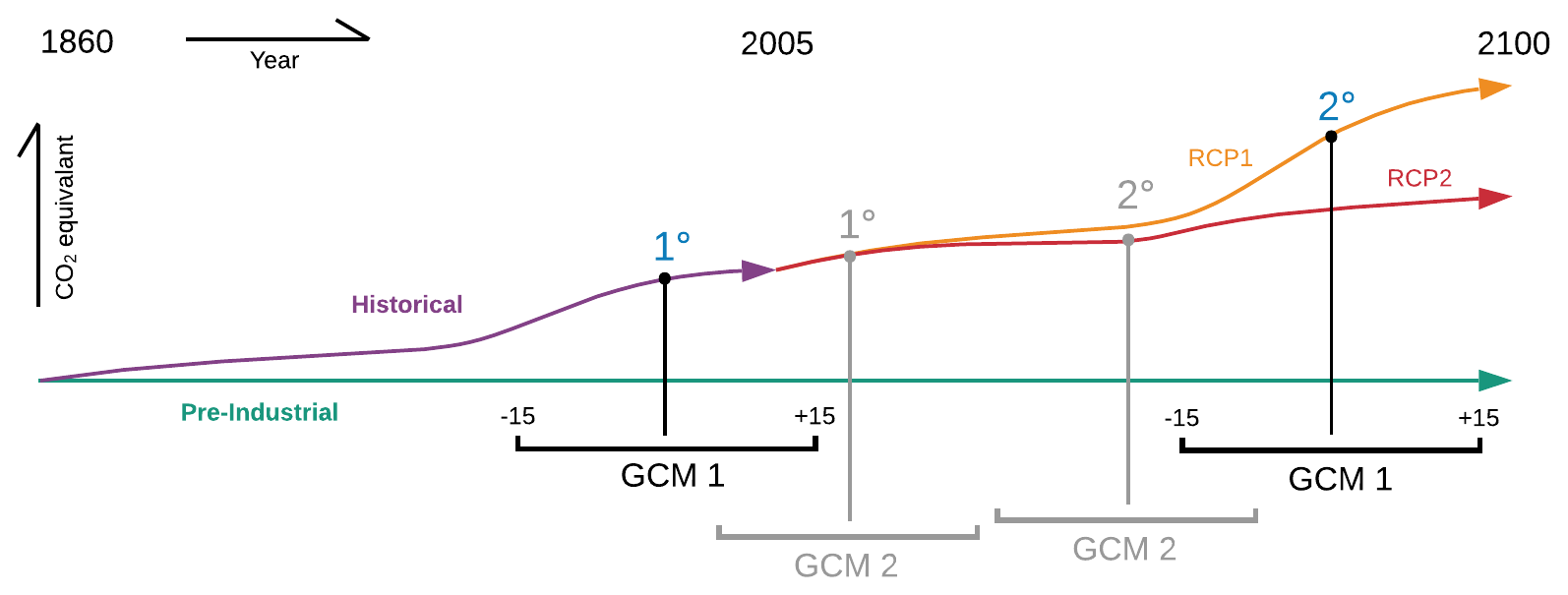
Figure 1Conceptual representation of how GW levels are determined for different GCMs, RCPs, and the PI comparison period.
Table 2Overview of the warming levels and in which year they are reached in the corresponding GCM (ISIMIP, 2019).

Considering that not all RCP/GCM combinations reach higher warming levels (Table 2), not all ensembles have the same size. Theoretically, the maximum ensemble size is 96, with a combination of 8 GHMs, 4 GCMs, and 3 RCPs (2.6, 6.0, and 8.5). Because projections under RCP8.5 were not available for PCR-GLOBWB, the maximum ensemble size is 84. The smallest ensemble (for 3∘C) consists of 36 members.
2.4 Calculation of model variance
To calculate whether the variance in absolute GWR change is mainly introduced through the GHMs or the GCMs, the following equation was applied per model grid cell and GW level.
where is the variance ratio of GCMs to GHMs, is the average variance of GWR change of all GHMs per GCM per RCP, and is the average variance in GWR change of all GCMs per RCP per GHM. The variance relative to the choice in RCP can be calculated similarly as follows:
where is the average variance in GWR of all RCPs per GCM per GHM.
2.5 Determining significant changes
A model ensemble allows us to consider the uncertainty in modeling physical processes as different models use different algorithms and parameters for computing groundwater recharge. To determine whether changes in GWR due to GW computed by the model ensemble are statistically significant, we used the two-sample Kolmogorov–Smirnov (K–S) test to compare the GWR values computed by all GHM–GCM model combinations under, for example, PI conditions with the values at the various GW levels. The use of a two-tailed t test is not advisable in this setting due to the small sample size (max. 84 in this study). Because the K–S test does not allow us to check whether the ensemble agrees on the sign of change in GWR, we applied an additional criterion to determine a significant change similar to Döll et al. (2018). A change is only marked as statistically significant if the K–S test indicates a significant difference and at least 60 % of the model realizations of the ensemble (RCP, GCM, and GHM combinations) agree on the sign of change (i.e., a decrease or increase). In case of a low significance, all models may show large responses to climate change while their agreement on the amount or sign of change is low.
3.1 Changes in groundwater recharge at different warming levels
To assess the impact of GW on GWR, Fig. 2 shows the ensemble mean change of GWR between the current 1∘C world and a potential 3∘C GW. We chose to express changes as absolute change rather than relative change because zero, or close to zero, GWR in some regions of the world leads to undefined or extremely large percentage increases and decreases (Figs. S1 and S2 in the Supplement). The model mean shows large decreases of over 100 mm per year in South America and in the Mississippi Basin and decreases of up to 50 mm per year in the Mediterranean, East China, and West Africa. Increases of over 100 mm per year are prominent in Indonesia and East Africa. Individual GHM–GCM model combinations compute much larger changes.
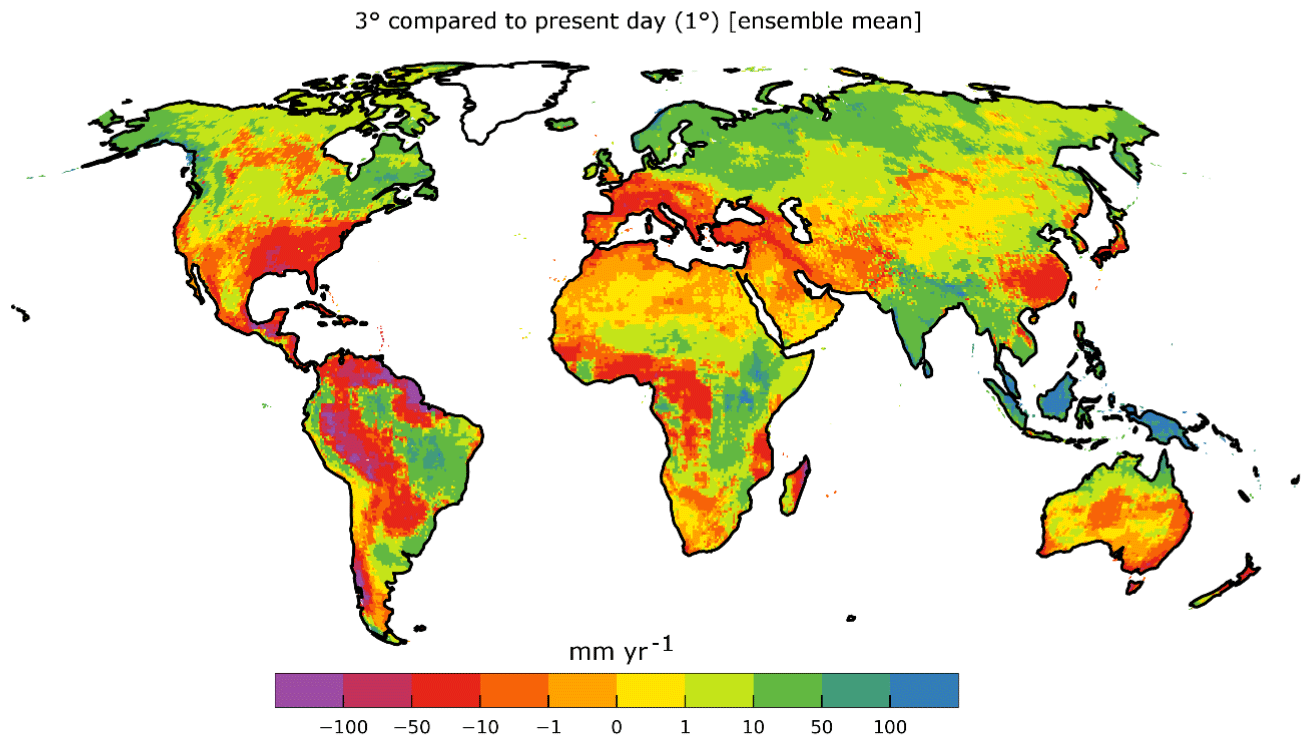
Figure 2Ensemble mean change in GWR (mm yr−1) between conditions of present-day warming of 1∘C GW and at 3∘C GW, averaged over the GWR changes of all GHM–GCM model combinations.
Ensemble mean changes, as shown in Fig. 2, may be low in some areas, but this could be due to large positive changes computed by some GHM–GCM model combinations being canceled by large negative changes by other model combinations. To assess the changes which show a high statistical agreement between the model combinations, we determine where computed changes of GWR are statistically significant (Sect. 2.5). As a reference for the intensity of the changes, Fig. 3a shows the mean GWR at PI averaged over all GHMs, RCPs, and GCMs from 1861 to 2099. The spatial pattern of GWR roughly agrees with the pattern of Mohan et al. (2018), which is derived by inferring it from more than 700 small-scale GWR estimates. The global mean GWR for the PI period is 140 mm per year, which is very similar to the value of 134 mm per year determined by Mohan et al. (2018) for the period 1981–2014 (see also Sect. 4).
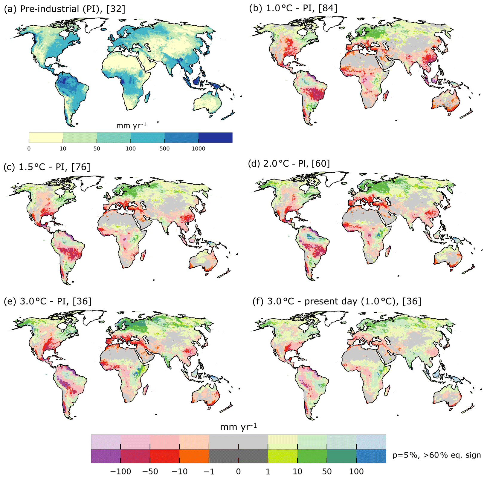
Figure 3Mean GWR (mm yr−1) for pre-industrial greenhouse gas concentrations, averaged over the GWR of all GHMs and GCMs (a). Ensemble mean absolute change in GWR (mm yr−1) at 1.0∘C (b), 1.5∘C (c), 2.0∘C (d), and 3.0∘C (e) GW compared to PI. The ensemble mean absolute change in GWR (mm yr−1) for 3.0∘C GW compared to GWR at the current GW of 1∘C (f). For (b) to (f), only those cells are displayed in solid colors where the Kolmogorov–Smirnov (K–S) test with a p of 5 % indicated that the ensemble GWR distribution for PI (for (f) the GWR distribution at 1∘C) and for the GW level difference, and at least 60 % of the models agree on the sign of the change. The ensemble size is shown in brackets. Lighter colors (upper color bar) show (statistical) insignificant mean differences.
Figure 3b–e show the (statistical) significant (bright colors; Sect. 2.5) mean absolute changes in GWR of the multi-model ensemble under a GW of 1.0, 1.5, 2.0, and 3.0∘C compared to PI, i.e., GWR of the PI runs for the corresponding time slices (Sect. 2.3). For all GW levels compared to PI (Fig. 3b–e), consistent patterns of decreasing GWR emerge for southern Chile, Brazil, central continental USA, the Mediterranean, and East China. Consistent and significant increases can be observed for northern Europe and in general northern latitudes and East Africa. Significant changes could only be derived for a small percentage of the total grid cells. Only about 15 % of the cells, on average for all GW levels, show significant increases or decreases. However, the patterns of non-significant (light colors) mean changes are consistent with the significant changes and show, for example, larger areas of increases and decreases around the significant changes for the Amazon. The identification of non-significance in most areas is due to the K–S test. The sign criterion affects mainly the Sahara and central Asia.
At 1∘C, GW (Fig. 3b) decreases of more than 100 mm per year are simulated in Southeast Asia, East China, Guyana, and southern Brazil. Decreases between 100 and 50 mm per year can be seen in central continental USA, southern Brazil, southern Chile, the Mediterranean, central Africa, and East China. Increases in GWR of 50 and over 100 mm per year are visible in the center of the Amazon, while decreases show in the northeastern and southern part that increase with GW. Overall, the significant global change is −17 mm per year at 1∘C.
A 1.5∘C GW shows only a limited increase in the Amazon but similar increases in the rest of the world. Decreases in GWR over 100 mm per year are now visible in Central America, but decreases for Southeast Asia have vanished. Smaller decreases, for example, in Australia, have also vanished in a 1.5∘C world. These effects are not necessarily due to no changes in GWR but due to disagreements in the ensemble that do not allow us to determine a reliable and significant change for this warming level. The global significant mean change is −12 mm per year at 1.5∘C GW.
At 2∘C GW, increases in GWR over 100 mm per year are present in northern Java, the Amazon, and East Africa. Decreases are similar to 1.5∘C GW, except for southern Chile and the northern Andes, where decreases become more severe. However, on the significant global mean, these changes balance out to −1 mm per year .
In a 3∘C world, large areas of decreases in GWR of over 100 mm per year in the Amazon Basin close to the Andes occur, and this is also the case in Guyana, Venezuela, West Africa, and the Mississippi Basin. Increases in GWR of over 100 mm per year, in contrast, are visible in East Africa, India, and northern Java. Increases of 50 to 100 mm per year dominate in northern latitudes at 3∘C warming compared to other GW levels. The global significant mean increases by +3 mm per year .
We have already reached a GW of approximately 1∘C (IPCC, 2018). Figure 3f shows the changes in GWR of a 3∘C GW compared to the present-day GW of already 1∘C instead of the PI. Overall, the agreement among the models is smaller than when the 3∘C world is compared to PI. Only 8 % of the cells show significant changes. Decreases over 100 mm per year are present in the Amazon Basin close to the Andes and on the coast of Guyana. Decreases of 50 to 100 mm per year are visible in Chile, the Mississippi Basin, the Caribbean, and southern France. Increases in GWR are again to be expected in the northern latitudes, southern Brazil, East Africa, and Southeast Asia, whereas the latter shows increases over 100 mm per year for Malaysia. The global significant mean change is +8 mm per year. Figure S3 shows the mean and median changes of GWR per latitude for all four GW levels, together with the standard deviation without a significance test. A decrease in mean GWR can be observed for all GW levels at 40∘ S, around 20∘ S (i.e., Namibia and Australia), and 5∘ N (Guyana). Increases are visible at 60∘ N (northern Europe) and in the south, close to the Equator, presenting a large spread and sudden change in direction in the tropics. Increases at greater than 60∘ N are likely due to a combination of different rain and snow patterns and snowmelt timing.
Large areas of insignificant changes of GWR (light colors) in Fig. 3 can be traced back to the uncertainty in GWR in between GHMs and GCMs. Figure 4 shows absolute GWR changes in a 1.5∘C world compared to PI (Fig. 4a and b) and the absolute GWR at PI (Fig. 4c and d) for the SREX (Special Report on Managing the Risks of Extreme Events and Disasters to Advance Climate Change Adaptation; Murray and Ebi, 2012; see Fig. S6 for a map of the SREX regions) region of the Amazon (left) and southern Europe/Mediterranean (right). Corresponding plots for all other SREX regions are provided in the Supplement. Similar to box plots, the letter-value plots in Fig. 4 show the distribution of values among the 0.5∘ grid cells belonging to the SREX region. Letter-value plots have the advantage of showing the distribution of values outside of the usual interquartile range (IQR; Q25–Q75). For example, for Fig. 4b CLM 4.5 with GFDL-ESM2-ES, the mean change in GWR is −19 mm per year, the middle box represents the IQR showing that 50 % of changes are close to zero or smaller than zero, the smaller box towards the negative changes shows that 12.5 % are smaller than −47 mm per year, whereas the additional missing box in the positive direction hints that almost no values are larger than zero. The horizontal size of the boxes is automatically scaled and does not carry any additional information.
Computed changes vary strongly among both GHMs and GCMs (Fig. 4a and b). In the Amazon, JULES-W1 shows a mean increase of 225 mm per year. Compared to WaterGAP2, JULES-W1 estimates of GWR change are 147 mm per year higher for MIROC5 and 44 mm per year lower for HadGEM. These differences are even large relative to the higher mean PI GWR in the Amazon compared to other regions of the world (compare to MED in Fig. 4). Nevertheless, the PI estimates also differ by, for example, 122 mm per year between JULES-W1 and WaterGAP2 on the mean for all GCMs and RCPs, and PI GWR is 625 mm per year smaller for H08 than for MATSIRO in the Amazon.
In the Mediterranean, almost all GHMs show the largest decreases in GWR with IPSL-CM5a-LR, followed by GFDL input, while HadGEM results in almost no change. However, the changes computed with each GCM input vary strongly among the GHMs. In general, CLM 4.5 and PCR-GLOBWB project the most considerable changes. The decrease in GWR computed by CLM 4.5 with IPSL-CM5a-LR is 33 % of the mean GWR calculated for PI with that model combination.
Conversely, JULES-W1 simulates for most grid cells in this SREX region the smallest PI GWR values (but also very high outliers) and, likely related, the smallest (mean) changes, together with MATSIRO and CWatM, which show altogether small GWR changes in all grid cells of the SREX regions. H08 and WaterGAP2, which apply similar approaches to modeling GWR as a function of total runoff, show somewhat similar GWR changes.
The four GHMs that take into account the impact of increasing CO2 (Sect. 2.1) do not result in similar changes as compared to the other four models. It is to be expected from the literature (Davie et al., 2013) that, with the physiological effect, the decreases in GWR would be slighter in the case of the CO2-sensitive models, but that is not the case. This is likely due to the approach of analyzing GW levels instead of RCPs and periods because different GCMs reach a particular GW level at different times and CO2 levels. This is further investigated in Sect. 3.3. On the global mean and for 1.5∘C GW, LPJmL simulates the lowest PI GWR, whereas MATSIRO and CLM 4.5 produce the highest global mean GWR (Fig. S4). PCR-GLOBWB simulates the largest global mean decreases with HadGEM (Fig. S5). In contrast, JULES-W1 and MATSIRO simulate increases of GWR on the global mean for all GCMs except for HadGEM (Fig. S5).
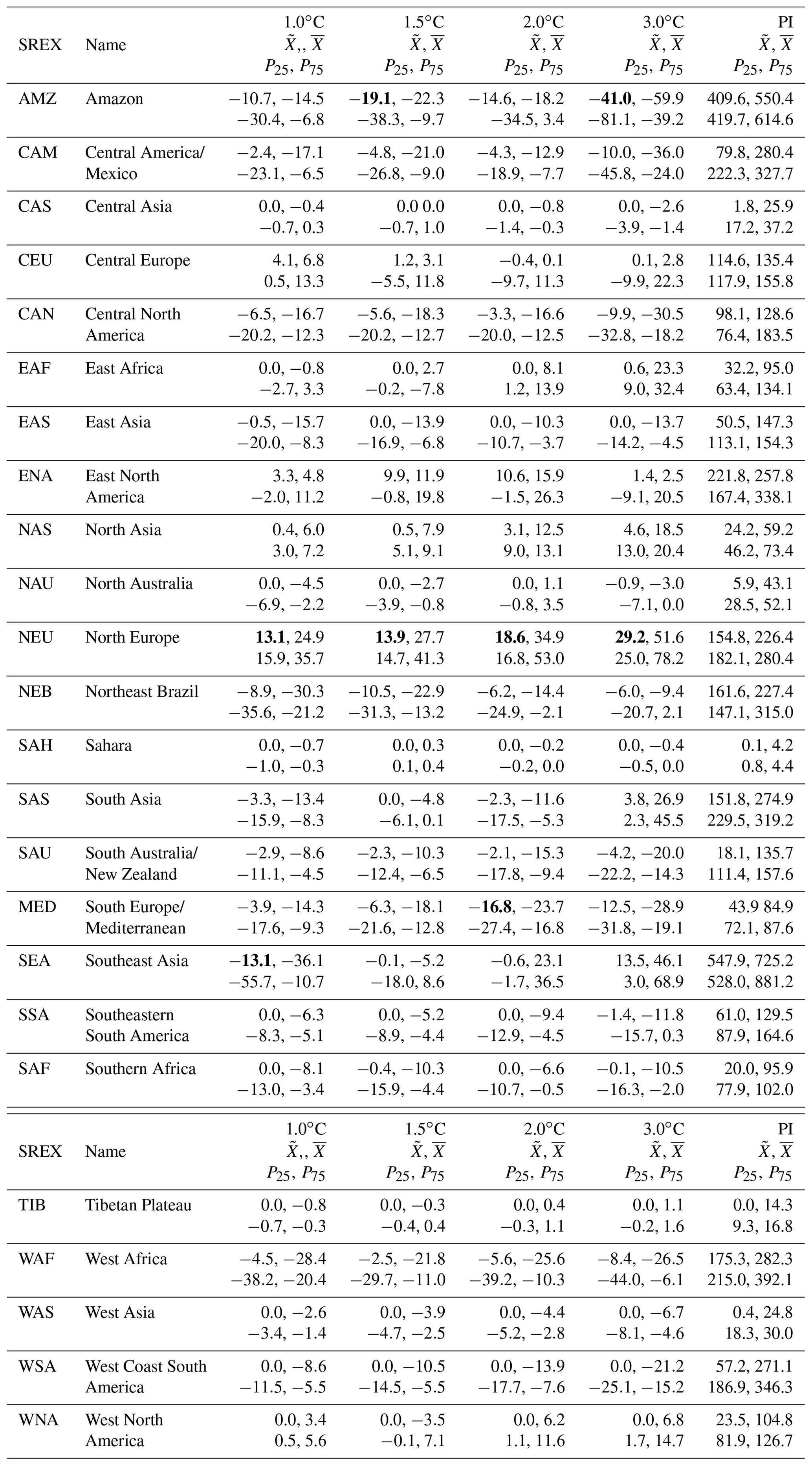
To provide an overview of changes in GWR in each SREX region, Table 3 shows the median, mean, and P25 and P75 changes in GWR compared to PI for all regions (see Fig. S6 for a map of the SREX regions). Overall, northern Europe shows the largest consistent increases in GWR, whereas the Amazon shows the largest consistent decreases, except for 2∘C, where southern Europe/Mediterranean shows the largest decreases of 18.6 mm per year as the median. For 3∘C, the Amazon shows the highest decreases in GWR with −41.0 mm per year as median. Notably, Southeast Asia first shows decreases of 13.1 mm per year with 1.0∘C GW and then no change with 1.5 and 2∘C and an increase in GWR of 13.5 mm per year with 3∘C. Relative to PI, the changes in the 3∘C GW in the the Amazon only account for 10 % of the GWR, compared to the 19 % relative increase of GWR in northern Europe with 3∘C and the 40 % decrease in GWR in southern Europe/Mediterranean at 2∘C GW.
Table 3Median (), mean (), P25, and P75 of absolute GWR change (mm yr−1) for four warming levels for each SREX region compared to PI. , , P25, and P75 describe the distribution of changes of spatially averaged GWR in each SREX region among all 36–84 ensemble members (Sect. 2.3). are the 25th and 75th percentile in the ensemble for a given region and a given GW level. The last column shows absolute GWR at PI. The following regions are not included due to the coarse spatial resolution of the models and low confidence in the reliability of results: the Arctic, Canada, Greenland, and Iceland, Antarctica, the Pacific islands, the southern tropical Pacific, the small island region of the Caribbean, and the West Indian Ocean. Maximum and minimum values per GW level are given in bold. No statistical test is applied to filter the values.
3.2 Sources of ensemble variance
To investigate whether the main variance in projected GWR changes is caused by GHMs, GCMs, or the different RCP scenarios, we apply Eqs. (1) and (2) (see Sect. 2.4) for 1.5 and 3∘C GW. Figure 5 shows the GCM to GHM variance ratio for 1.5∘C (Fig. 5a) and 3∘C (Fig. 5b) per grid cell; the GHM RCP variance ratio is not shown here (see Fig. S7; mean of GHM RCP ratio – 22 %) as the primary influence can be appropriated to the GCM and GHM selection (this is also the case when choosing only the CO2 sensitive models). For the simulated variance at PI, see Figs. S1 and S4.
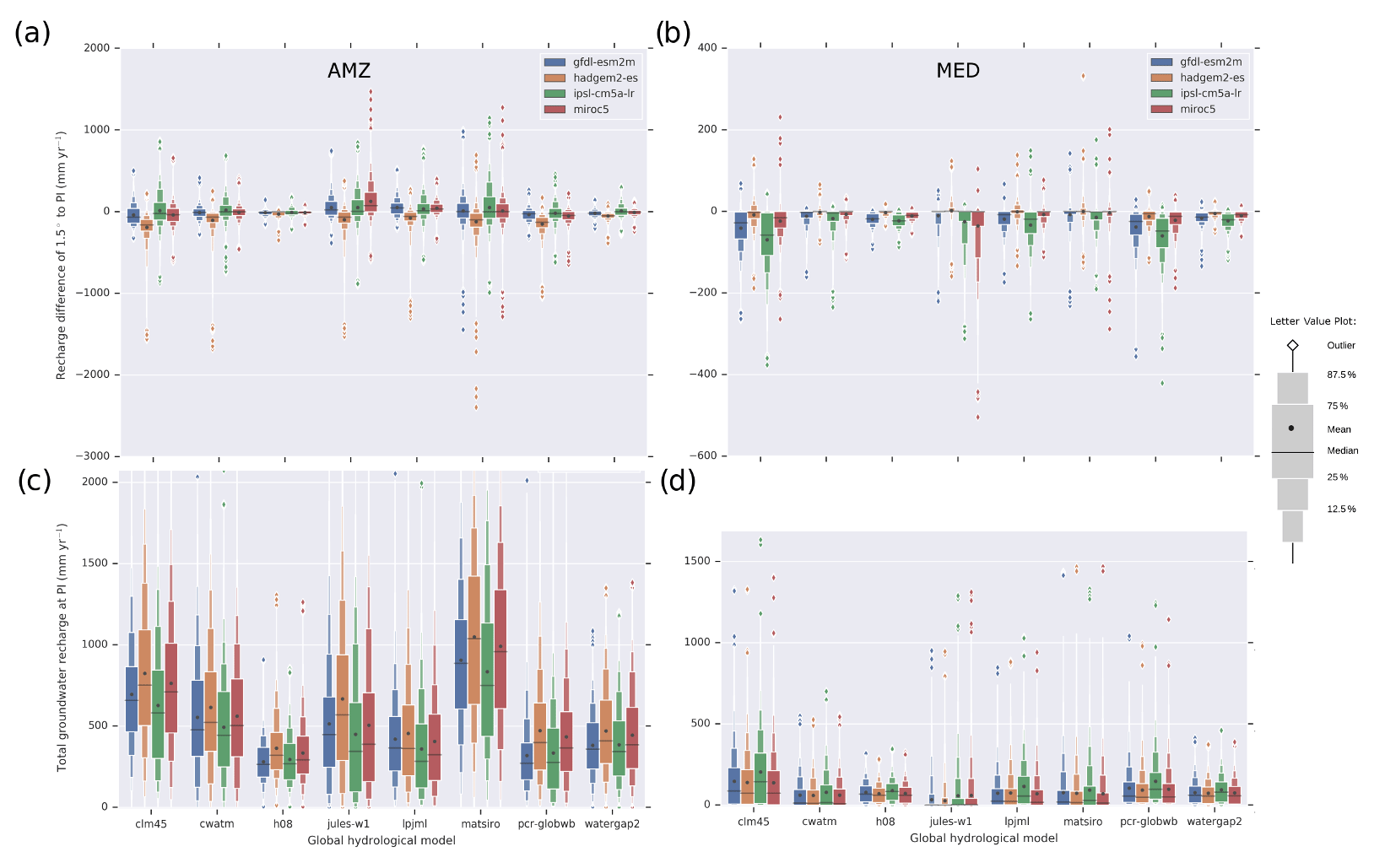
Figure 4Letter-value plot (Hofmann et al., 2017) of absolute changes in GWR in 0.5∘ grid cells (mm yr−1) at 1.5∘C GW compared to PI (a, b) and absolute PI GWR (mm yr−1) (c, d) for the Amazon (a, c) and the southern Europe/Mediterranean (b, d) SREX region (for all other regions and GW levels (2, 3∘C), see the Supplement). No statistical test is applied, and all grid cells inside a region are included. Each box may include multiple simulations with different RCPs.
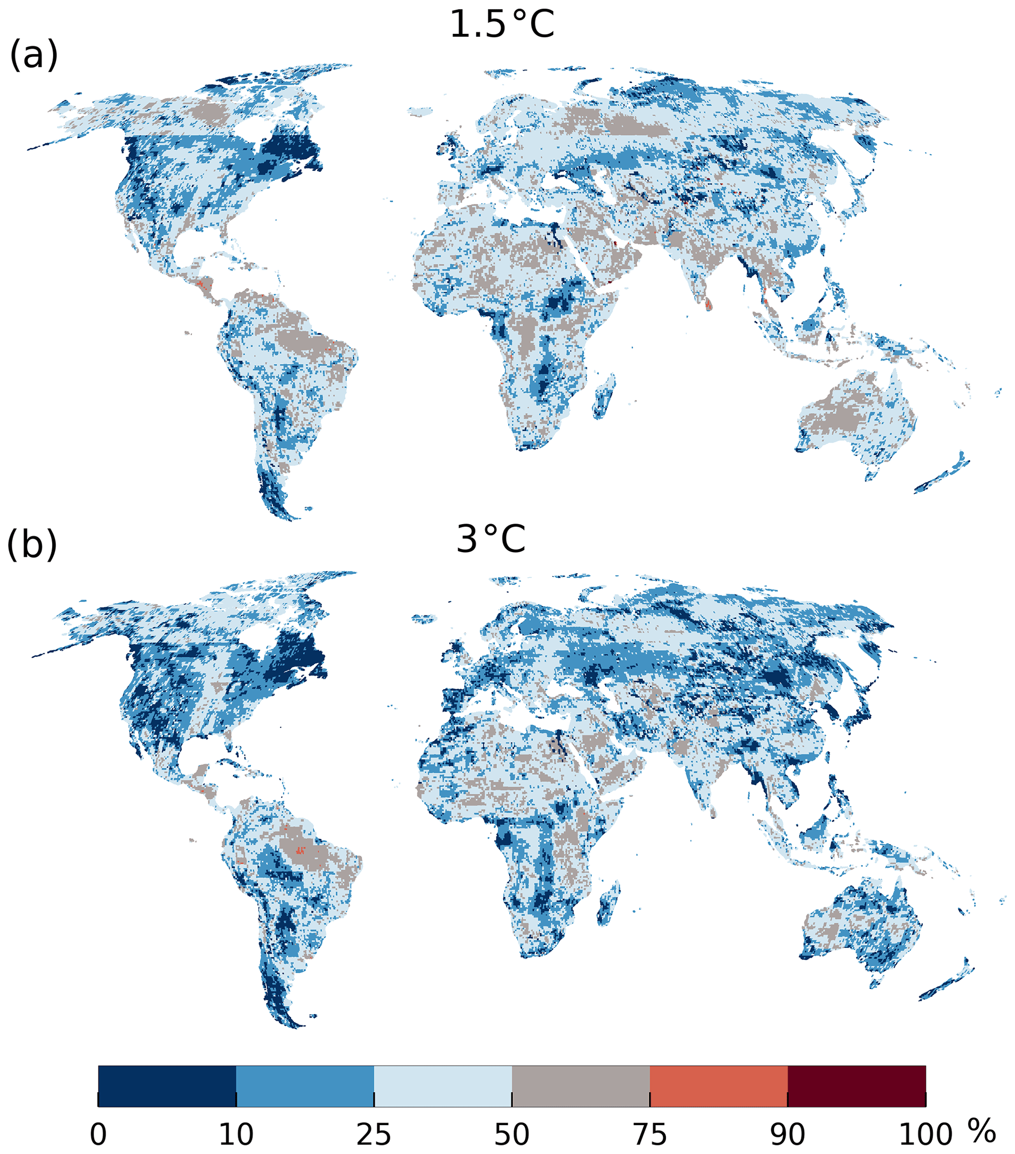
Figure 5GCM variance in percent of the total variance of GWR change from eight GHMs and four GCMs at 1.5∘C (a) and a 3∘C (b) GW (see also Sect. 2.4). Red depicts areas where the GCMs are responsible for the majority of the variance in GWR change. Blue areas indicate where the main variance is introduced through GHMs.
Overall, GHMs cause more significant variance in 1.5∘C than in a 3∘C world, which is plausible because of increased GCM trends with increased CO2 concentrations. This is possibly also due to the missing RCP8.5 simulations for PCR-GLOBWB for all GCMs. A clear spatial pattern of GCM influence in the Amazon shows that it relates to the region of Fig. 3 where increases of GWR are calculated. On the other hand, the region in the Amazon where decreases are simulated (see Fig. 3) shows mainly the GHMs as the source of variance. In the Mediterranean, the influence shifts as well from GCMs (1.5∘C) to GHMs (3∘C). This could be due to a high agreement in GCMs in this region and a considerable disagreement in GHMs. Similar patterns can be found when comparing absolute GWR, but the influence of GCMs is less pronounced, especially in the Amazon (Fig. S8).
3.3 Impacts of evolving carbon dioxide concentrations on groundwater recharge estimates
Including vegetation dynamics in GHMs may alter the model response in future estimates of GWR as evolving CO2 concentrations alter the fluxes of energy and water (Davie et al., 2013). To investigate the influence of simulating the physiological impacts of evolving CO2 on GWR, we compared GWR changes computed by two CLM 4.5 runs, each of which were driven by GFDL-ESM2M climate input; the standard run included the ensemble analysis above, with CO2 concentrations changing according to the RCP, and an additional run was done in which CO2 concentrations after 2005 were held constant at the 2005 level. Unfortunately, no other GHM–GCM combinations with these alternative CO2 concentration variants are available in the framework of ISIMIP2b.
Figure 6 shows differences in simulated GWR between a dynamic and a static CO2 simulation for 2∘C (Fig. 6a) and 3∘C (Fig. 6b). In most grid cells, GWR simulated with dynamic CO2 is larger than GWR simulated with static CO2 levels of 2005 (Fig. 6a and b). In the tropics, GWR with dynamic CO2 can be higher than with constant CO2 by 10–50 mm per year for 2∘C GW (Fig. 6a), while difference reaches 50–100 mm per year in the 3∘C world (Fig. 6b). Decreases in GWR are spatially consistent (for example, in Brazil, Central US, and India) at 2 and 3∘C GW and rarely exceed 10 mm per year.

Figure 6GWR (dynamic CO2) compared to GWR (static CO2; mm yr−1) for 2.0∘C (a) and 3.0∘C (b) GW. GWR (dynamic CO2) compared to PI (dynamic CO2; mm yr−1) for 2.0∘C (c) and 3.0∘C (d) GW. The figure only includes the GHM CLM 4.5 and the GCM GFDL-ESM2M. Maps show changes in GWR at a certain GW (including all RCPs that lead to that GW with a certain CO2 concentration), with dynamically evolving CO2 compared to static CO2 concentrations from 2005. Green and blue mean that GWR is higher when evolving CO2 concentrations are considered; red and purple indicate lower GWR.
Compared to the absolute changes between PI and the GW levels for dynamic CO2 (Fig. 6c and d), the decreases in GWR are rather small (e.g., up −10 mm per year in Brazil (see Fig. 6a and b), while change compared to PI exceeds −100 mm per year; see Fig. 6c and d). Also, increases in GWR due to dynamic CO2 are in regions with large (>100 mm per year; see Fig. 6c and d) increases in recharge.
The preceding analysis focused on GW levels parallel to other studies of GHM ensembles. To investigate the difference in including active vegetation processes in GHM further, we compared the four GHMs that include these processes with the four models that do not (Table 1). Because different RCPs decide the concentration of CO2 in the atmosphere, we compare RCP2.6 and RCP8.5 time slices instead of GW levels.
Figure 7 compares the precipitation and GWR changes between the period 1981–2010 and the period 2070–2099 for the two RCPs, and the two different model types for the SREX regions investigated in Table 3. Changes in precipitation and GWR are only based on the GCM HadGEM2-ES (see Fig. S9 for the average over all GCMs) as the relationship between GWR and precipitation is not linear, and the plot is comparable to Davie et al. (2013), who investigated differences in runoff. Compared to the average precipitation of all GCMs where only two regions show a decrease larger than 100 mm per year (Fig. S9b), HadGEM2-ES shows seven regions for RCP8.5 with such a decrease in precipitation.
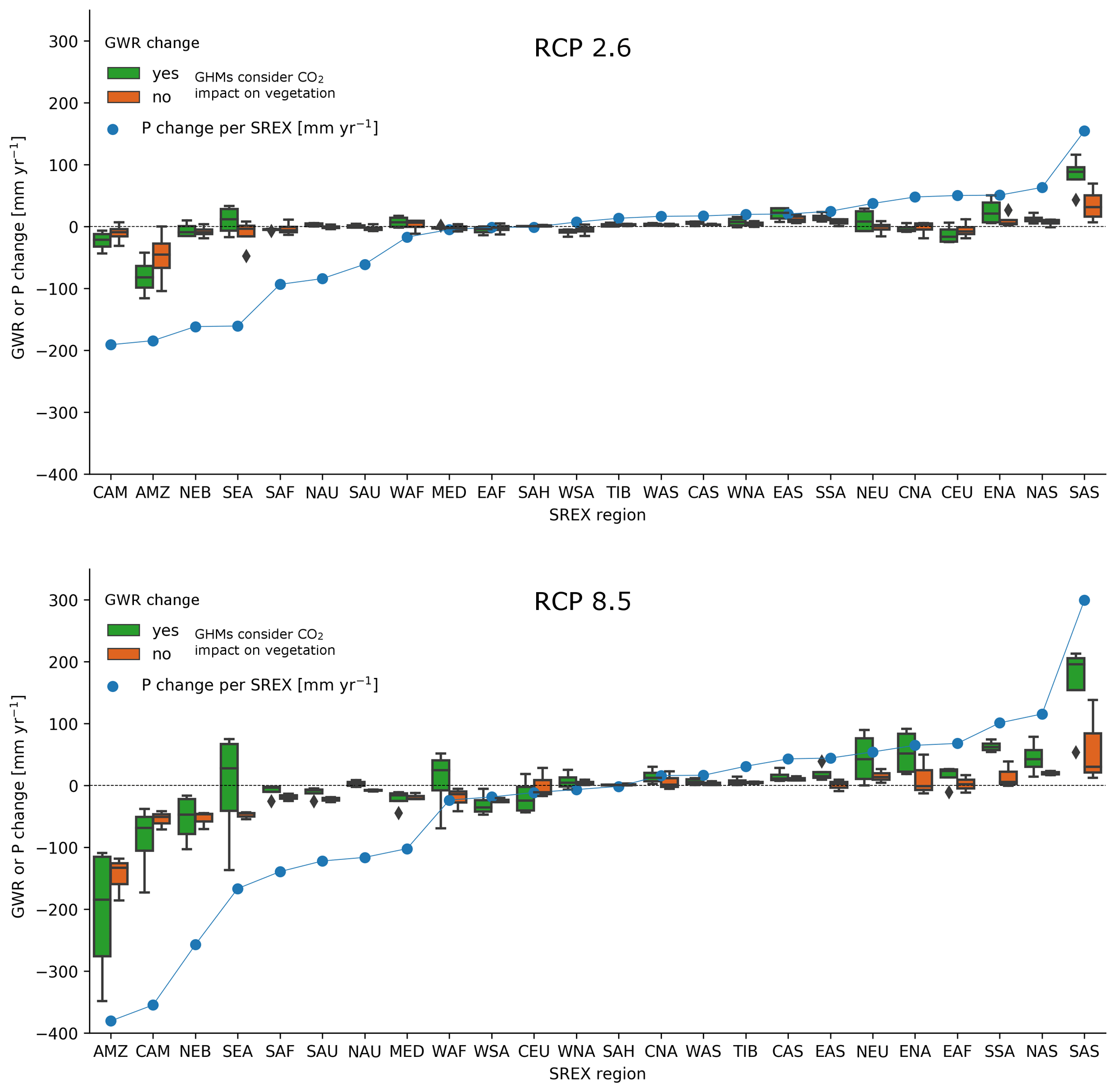
Figure 7Relation of changes in precipitation (P; means from 1981–2010 to 2070–2099) to changes in GWR (means from 1981–2010 to 2070–2099), depending on the model type (with or without CO2; see also Table 1) per SREX (selection as in Table 3) for RCP2.6 and RCP8.5 for the GCM HadGEM2-ES.
GWR changes vary between RCPs and model type and in between GHMs (Fig. S10). The relation between precipitation and GWR and the difference between model types becomes clearer with RCP8.5 than with RCP2.6. Models with active vegetation (Fig. 7; green markers) agree that with more precipitation GWR should increase, for example, for South Asia (SAS); however, they disagree in regions where decreases in precipitation are expected and the risk for groundwater availability is highest, for example, Central America (CAM) and South Europe/Mediterranean (MED). GHMs without active vegetation (Fig. 7; orange markers), on the other hand, show a more consistent decrease in GWR for regions with decreases in precipitation and only some agreement in regions with increased precipitation.
Decreases in precipitation may lead to a decrease in vegetation productivity (if not counteracted by an increased water use efficiency due to elevated CO2 concentrations; Singh et al., 2020) and, thus, to a decrease in transpiration. GHMs assume shares for evapotranspiration (ET) in relation to potential ET and the available precipitation. In contrast, transpiration in CO2-driven models responds to active vegetation and the relations between different water flux components that simpler GHMs do not. This can explain why the dynamic vegetation models exhibit inter-model regional differences in the GWR response to P decrease. Furthermore, some models (MATSIRO) may not calculate LAI which impacts transpiration. For models with active vegetation, the increase in water use efficiency due to stomatal conductance (also referred to as CO2 fertilization) can compensate for the decrease in precipitation to some extent, making more water available for groundwater recharge as compared to the GHMs (Table 1). Though, in some regions, as seen in Fig. 7 (and Fig. S10), this feedback is not enough to overcome the warmer and drier climate in terms of groundwater flux. Overall, the capability of a model to simulate actual ET largely influences its capability to simulate groundwater recharge.
CWatM often lies in the middle of simulated GWR changes at RCP2.6. Davie et al. (2013) showed generally higher runoff values for JULES-W1 than for LPJmL; the reverse is true for GWR (Fig. S10). For RCP8.5, CWatM always simulates the largest increases and lowest decreases in GWR of all models without active vegetation.
A spatially more refined difference between the model types is shown in Fig. 8 for RCP8.5 (for RCP 2.6, almost no significant changes were found). For each grid cell, the map shows the significant (K–S test; p is 5 %) absolute difference in simulated change in GWR between models that include dynamic vegetation processes and models that do not include them. In the northern latitudes, both models with and without dynamic vegetation agree on an increase in GWR but differ by up to 100 mm per year. Similarly, in the Mediterranean and central Brazil, both model types simulate a decrease in GWR, but the magnitude is significantly different between the model groups. In the Amazon, patches of significant differences between the models show increases in GWR computed by GHMs with dynamic vegetation, whereas GHMs without dynamic vegetation show a decrease. A similar effect is visible in central Africa, India, and parts of Indonesia; however, decreases are also simulated instead of increases for the Congo and Zambezi catchment. Both in the Mediterranean and South America, models with dynamic vegetation show up to 100 mm per year difference in change compared to models without – even though no physiological effect should be dominant. According to Fig. 6, this is likely due to CLM 4.5 because JULES-W1 and LPJmL show a slighter GWR decrease than the models without dynamic vegetation. It is likely that the shown differences are due to the implementation of dynamic vegetation in the GHMs (see Fig. S10); however, it is possible that other model peculiarities and processes are relevant as well.

Figure 8Significant absolute difference in GWR change between 1981–2010 and 2077–2099 for RCP8.5 in between four GHMs with (dyn) and four GHMs without dynamic (or active) vegetation (no dyn). See also Table 1. A reddish color (left side of the color bar) indicates that the mean change in GWR, as computed by the models with dynamic vegetation, is more negative or less positive than change computed by other models. White regions indicate no significance is based on the K–S test (Sect. 2.5). Solid colors indicate that the majority of the two model groups (three out of four models for each group) do not have the same sign; i.e., that including dynamic vegetation leads to different signs in the GWR change. Lighter colors indicate where the majority agrees on the sign of change.
Estimating GWR is challenging (Moeck et al., 2016). Our results show that, even for the PI period, the estimates of GWR vary largely among different GHMs. This is likely caused by the very different treatment of the runoff partitioning, implementation of the soil layer(s), inclusion of dynamic vegetation processes, and simulation of capillary rise. Because GWR is hard to measure directly (Scanlon et al., 2002), it is also challenging to verify the accuracy of the estimates.
To the best of our knowledge, the data set of Mohan et al. (2018) is the only available gridded global GWR data set that is not based on global hydrological modeling. This data set of mean 1981–2010 GWR in 0.5∘ grid cells was developed from a regression analysis that combined gridded data sets of mean precipitation and potential evapotranspiration and land use and/or land cover with local estimates of GWR at 715 locations worldwide. Figure 9 compares the GHMs under investigation for PI conditions to this data set. The used data for comparison are one ensemble member of the analysis of Mohan et al. (2018) that was deemed best in their study. The global mean GWR in this member is slightly lower, at 110 mm per year, than the reported mean of 134 mm per year. Overall, the GHMs best agree with Mohan et al. (2018) in arid regions like the Sahara, Australia, southern Africa, and the Andes. Underestimates are predominant in the northern latitudes and Central Asia, whereas underestimates appear in Europe and the eastern USA for all models. All models, except for H08 and WaterGAP2 which show underestimates, result in overestimates in East Asia. In the Amazon, MATSIRO and CLM 4.5 overestimate by more than 100 mm per year compared to Mohan et al. (2018), whereas all other models show a mix of over- and underestimates across continents. A similar pattern is visible in central Africa, where CLM, MATSIRO, and CWatM overestimate, and all other models show a mixture of over- and underestimates of −100 to 100 mm per year. H08 and WaterGAP2 have the best agreement according to the NSE (Nash–Sutcliffe efficiency; calculated spatially; Nash and Sutcliffe, 1970) of 0.4 and 0.2, while the bias (mean (GHM Mohan et al.)) is lowest for JULES-W1. All GHMs show much lower GWR in permafrost regions as they assume that there is no or little GWR in such regions. It is possible that the GWR of Mohan et al. (2018) is overestimated here as no measurements informed their results in these regions.
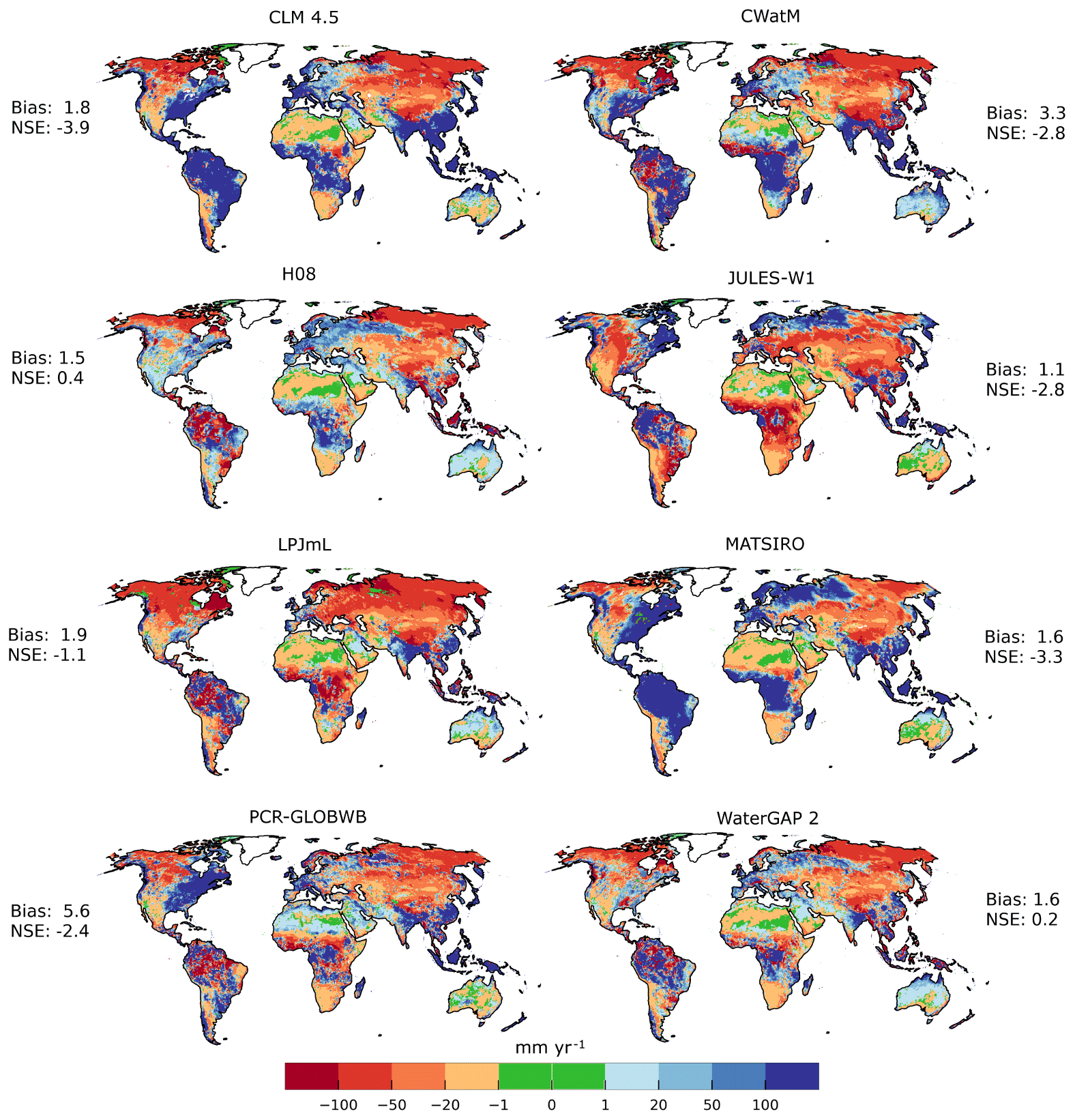
Figure 9PI GWR per GHM compared to the 34-year (1981–2014) mean GWR (mm yr−1) of Mohan et al. (2018). Bias is the mean (GHM Mohan et al. 2018). NSE (Nash–Sutcliffe efficiency; Nash and Sutcliffe, 1970) is calculated spatially over all cells instead of time.
The variance in modeled GWR is possibly caused by the different implementation of the hydrological processes in between the models. Furthermore, models differ in their definition of groundwater and GWR. Some include groundwater storage that is recharged by a fraction of precipitation; others do not include a groundwater component at all but define the saturation of excess water from the bottom soil layer as GWR. Models may include only some of the processes that affect GWR, for example, capillary rise, percolation from the soil, preferential flow bypassing the soil matrix, the interaction between surface water and the aquifer, changing land use over time (not considered here), and changing vegetation (e.g., reducing infiltration capacity). Furthermore, important processes like evaporation, infiltration, percolation, or runoff and GWR separation are implemented with different equations and simplifications. For evapotranspiration, a standard deviation of 0.15 mm per day globally for the period 1989–2005 was found in the ISIMIP ensemble (Wartenburger et al., 2018). Some models even use sub-grid information or sub-daily time steps, e.g., for changes in unsaturated conductivity. Notably, models that include dynamic vegetation processes showed the largest spread in GWR in regions with decreasing precipitation. It is also important to distinguish the capability of the models to compute groundwater recharge during a historical period from their capability to estimate changes in groundwater recharge due to climate change. A model that simulates the current groundwater recharge pattern correctly may be incapable of computing future groundwater recharge if it cannot correctly simulate the impact of climate change and changing atmospheric CO2 concentrations on actual evapotranspiration correctly.
To illustrate the model differences further, the following describes the impact of changes in precipitation for WaterGAP and LPJmL, which is representative for the different model types used in this study. In WaterGAP, a simulated percent change in total runoff translates to the same percentage change in GWR unless, for example, due to more extreme precipitation events, the infiltration capacity is exceeded more often – such that the relative increase in GWR is smaller than total runoff. Absolute changes in GWR are always smaller than changes in total runoff. In LPJmL, changes in total runoff do not translate to proportional changes in groundwater runoff and GWR. Any flux or storage that takes water before it is partitioned to the soil will impact the groundwater and GWR. Possible reasons for a reduction in GWR (percolation past the bottom hydrologically active layer at 3 m depth; see Sect. 2.1) can be changes in precipitation amount and/or intensity, transpiration due to vegetation productivity, transpiration due to changes in vegetation water use efficiency due to CO2 fertilization, or changes in anthropogenic water use demands.
This difference in behavior is reflected in Fig. 7, where the response between precipitation and GWR of GHMs without any active and/or dynamic vegetation is relatively uniform. The non-uniform response of the models that include vegetation changes is likely due to the complicated process feedbacks between vegetation and water (transpiration changes due to available water together with vegetation productivity) and complex feedbacks in between changes in CO2, temperature, and precipitation which affect vegetation.
This study highlights that uncertainties and differences in GHMs need to be investigated further, and that, in order to estimate global groundwater vulnerability, improved estimates of global GWR are required.
This study is limited not only by the uncertainty in correctly representing the process of GWR but also in the propagation and aggregation of uncertainties. Future greenhouse gas emission scenarios are created based on the input of integrated assessment models. They are translated into emission scenarios of atmospheric concentrations and forcings that are, in turn, used to evaluate their impacts on the climate simulated by GCMs. Outputs of the GCMs are then bias adjusted and spatially downscaled to be used in the assessment with impact models like GHMs (Döll et al., 2014a). Furthermore, the analysis is limited by the number of GCMs that were used, as discussed in McSweeney and Jones (2016), although the GCMs are carefully selected to be most representative of the CMIP (Taylor et al., 2012) ensemble.
The multi-model ensemble study presented here assesses GWR at GW of 1.5, 2, and 3∘C compared to GWR simulated under pre-industrial climate conditions and 1∘C of GW. Changes are assessed based on transient time slices of the 30 years around the year that crosses the specific warming level. These slices are an approximation of the stabilized climate state of that warming level; they rely on the assumption that, for a given warming level, the impacts are the same regardless of the time it took to reach it or whether equilibrium has been reached at all (Boulange et al., 2018). However, this kind of analysis has limitations as the transient nature of climate is aggregated over a relatively short period (31 years). Components like the ocean might not equilibrate at these timescales (Donnelly et al., 2017).
Additionally, different RCPs are combined, which limit the possibility to investigate processes that are sensitive to different CO2 concentrations. Investigations in this study based on RCPs show the difference between these model types. On the other hand, using GW levels reduces the uncertainties from GCM variability due to the use of different time slices, depending on when a GCM reaches a GW level.
The variance in GWR is caused by GCMs and GHMs alike, depending on the region similar to a multi-model ensemble study on the climate change impacts on streamflow (Schewe et al., 2014). Again, the assessment is limited by the number of used GCMs. Furthermore, this study did not include changes in land cover and land use and, thus, irrigation, which can have a tremendous impact on GWR, especially as irrigation patterns and used crops will change with a changing climate (Hauser et al., 2019; Hirsch et al., 2017, 2018; Thiery et al., 2017, 2020). The only similar study on the global impacts of GW on GWR, to the knowledge of the authors, was conducted by Portmann et al. (2013). The study used five GCMs and one GHM, WaterGAP, which (a slightly different version) was also included in this study. Overall results are spatially consistent; however, Portmann et al. (2013) showed more consistent trends among GW levels (compare Table 3). Portmann et al. (2013) acknowledge that including impacts of evolving CO2 levels on vegetation will have an impact on the simulated GWR and that WaterGAP is likely overestimating the decreases in GWR. Similarly, Davie et al. (2013) found that the simulation of runoff was not consistent across models, depending on whether CO2 was considered. The results presented in this study show that this assumption is true for some regions, where differences of up to 100 mm per year can be observed.
Despite the uncertainties, this study provides further evidence that climate change will impact groundwater availability in many regions of the world. A notable decrease can be expected in the Mediterranean, the Amazon, and Brazil, whereas increases can be expected in northern Europe. It is nevertheless troublesome that, especially in regions that are known to be vulnerable to climate change, for example, southern Africa, model agreement in between model types is low.
Potential GWR changes due to climate change require increased attention from the scientific community and from decision makers because they affect future water availability in many regions and, thus, the wellbeing of billions of people. This study shows that simulated global-scale estimates of GWR vary strongly among GHMs, which contribute more strongly to the overall uncertainty of future GWR than the applied GCM output. However, statistically significant increases and decreases in GWR could be identified in specific regions per GW level. The presented inter-model ranges of GWR changes are an important input for processes aiming at developing strategies for climate change adaptation, as risk-averse decision makers may want to orient their strategies towards adapting to the worst-case GWR change and not to the projected ensemble mean change.
This study shows that including vegetation processes in GHMs can change projected GWR changes substantially. However, consideration of these processes does not lead to a uniform increase in groundwater recharge, as might be expected from the physiological effect of increasing atmospheric CO2 concentration. In some regions with decreasing groundwater recharge, where groundwater availability is a major concern, models that include these processes show the largest differences among themselves. Further research is necessary to understand GWR on large scales and how it is affected by climate. Simulation of groundwater recharge in global models and the connected uncertainties needs to be analyzed in greater detail by, e.g., the application of extensive sensitivity analysis. Such an assessment should also extend to the benefit of integrating gradient-based groundwater flow models in GHMs.
All simulations are available through the ISIMIP project at https://www.isimip.org (last access: 1 January 2020) (Gosling et al., 2020).
The supplement related to this article is available online at: https://doi.org/10.5194/hess-25-787-2021-supplement.
RR led the conceptualization, formal analysis, methodology, software, visualization, and writing of the draft. The original idea was by HMS. HMS and PD supported the review and editing of the paper and the development of the methodology. TT supported the editing and review. MF, SNG, MG, NH, AK, LS, WT, YW, YP, BP, and SY contributed to the model description in Sect. 2 and made suggestions regarding wording, figures, and discussion. PD and HMS supervised the work of RR and made suggestions regarding the analysis, structure, and wording of the text and design of tables and figures.
The authors declare that they have no conflict of interest.
We would like to thank the ISIMIP (https://www.isimip.org, last access: 16 February 2021) project for supplying the data and the modeling community for carrying out these crucial simulations. We should, furthermore, like to thank Chinchu Mohan for providing the data.
This research has been supported by the German Federal Ministry of Education and Research (grant no. 01LS1711F). Yadu Pokhrel acknowledges support from the National Science Foundation (CAREER Award; grant no. 1752729).
This paper was edited by Philippe Ackerer and reviewed by five anonymous referees.
Alcamo, J., Döll, P., Henrichs, T., Kaspar, F., Lehner, B., Rösch, T., and Siebert, S.: Development and testing of the WaterGAP 2 global model of water use and availability, Hydrolog. Sci. J., 48, 317–337, https://doi.org/10.1623/hysj.48.3.317.45290, 2003.
Alfieri, L., Bisselink, B., Dottori, F., Naumann, G., de Roo, A., Salamon, P., Wyser, K., and Feyen, L.: Global projections of river flood risk in a warmer world, Earth's Future, 5, 171–182, https://doi.org/10.1002/2016EF000485, 2017.
Arnold, J. G., Williams, J. R., Nicks, A. D., and Sammons, N. B.: SWRRB; a basin scale simulation model for soil and water resources management, Texas A & M University Press, College Station, Texas, 142 pp., 1990.
Best, M. J., Pryor, M., Clark, D. B., Rooney, G. G., Essery, R. H., Ménard, C. B., Edwards, J. M., Hendry, M. A., Porson, A., Gedney, N., Mercado, L. M., Sitch, S., Blyth, E., Boucher, O., Cox, P. M., Grimmond, C. S. B., and Harding, R. J.: The Joint UK Land Environment Simulator (JULES), model description – Part 1: Energy and water fluxes, Geosci. Model Dev., 4, 677–699, https://doi.org/10.5194/gmd-4-677-2011, 2011.
Beven, K. J. and Kirkby, M. J.: A physically based, variable contributing area model of basin hydrology/Un modèle à base physique de zone d'appel variable de l'hydrologie du bassin versant, Hydrolog. Sci. Bull., 24, 43–69, https://doi.org/10.1080/02626667909491834, 1979.
Boulange, J., Hanasaki, N., Veldkamp, T., Schewe, J., and Shiogama, H.: Magnitude and robustness associated with the climate change impacts on global hydrological variables for transient and stabilized climate states, Environ. Res. Lett., 13, 64017, https://doi.org/10.1088/1748-9326/aac179, 2018.
Burek, P., Satoh, Y., Kahil, T., Tang, T., Greve, P., Smilovic, M., Guillaumot, L., Zhao, F., and Wada, Y.: Development of the Community Water Model (CWatM v1.04) – a high-resolution hydrological model for global and regional assessment of integrated water resources management, Geosci. Model Dev., 13, 3267–3298, https://doi.org/10.5194/gmd-13-3267-2020, 2020.
Byers, E., Gidden, M., Leclère, D., Balkovic, J., Burek, P., Ebi, K., Greve, P., Grey, D., Havlik, P., Hillers, A., Johnson, N., Kahil, T., Krey, V., Langan, S., Nakicenovic, N., Novak, R., Obersteiner, M., Pachauri, S., Palazzo, A., Parkinson, S., Rao, N. D., Rogelj, J., Satoh, Y., Wada, Y., Willaarts, B., and Riahi, K.: Global exposure and vulnerability to multi-sector development and climate change hotspots, Environ. Res. Lett., 13, 55012, https://doi.org/10.1088/1748-9326/aabf45, 2018.
Clark, D. B., Mercado, L. M., Sitch, S., Jones, C. D., Gedney, N., Best, M. J., Pryor, M., Rooney, G. G., Essery, R. L. H., Blyth, E., Boucher, O., Harding, R. J., Huntingford, C., and Cox, P. M.: The Joint UK Land Environment Simulator (JULES), model description – Part 2: Carbon fluxes and vegetation dynamics, Geosci. Model Dev., 4, 701–722, https://doi.org/10.5194/gmd-4-701-2011, 2011.
Collatz, G., Ball, J., Grivet, C., and Berry, J. A.: Physiological and environmental regulation of stomatal conductance, photosynthesis and transpiration: a model that includes a laminar boundary layer, Agr. Forest Meteorol., 54, 107–136, https://doi.org/10.1016/0168-1923(91)90002-8, 1991.
Cuthbert, M. O., Gleeson, T., Moosdorf, N., Befus, K. M., Schneider, A., Hartmann, J., and Lehner, B.: Global patterns and dynamics of climate–groundwater interactions, Nat. Clim. Change, 9, 137–141, https://doi.org/10.1038/s41558-018-0386-4, 2019a.
Cuthbert, M. O., Taylor, R. G., Favreau, G., Todd, M. C., Shamsudduha, M., Villholth, K. G., MacDonald, A. M., Scanlon, B. R., Kotchoni, D. O. V., Vouillamoz, J.-M., Lawson, F. M. A., Adjomayi, P. A., Kashaigili, J., Seddon, D., Sorensen, J. P. R., Ebrahim, G. Y., Owor, M., Nyenje, P. M., Nazoumou, Y., Goni, I., Ousmane, B. I., Sibanda, T., Ascott, M. J., Macdonald, D. M. J., Agyekum, W., Koussoubé, Y., Wanke, H., Kim, H., Wada, Y., Lo, M.-H., Oki, T., and Kukuric, N.: Observed controls on resilience of groundwater to climate variability in sub-Saharan Africa, Nature, 572, 230–234, https://doi.org/10.1038/s41586-019-1441-7, 2019b.
Davie, J. C. S., Falloon, P. D., Kahana, R., Dankers, R., Betts, R., Portmann, F. T., Wisser, D., Clark, D. B., Ito, A., Masaki, Y., Nishina, K., Fekete, B., Tessler, Z., Wada, Y., Liu, X., Tang, Q., Hagemann, S., Stacke, T., Pavlick, R., Schaphoff, S., Gosling, S. N., Franssen, W., and Arnell, N.: Comparing projections of future changes in runoff from hydrological and biome models in ISI-MIP, Earth Syst. Dynam., 4, 359–374, https://doi.org/10.5194/esd-4-359-2013, 2013.
de Graaf, I. E. M., Gleeson, T., (Rens) van Beek, L. P. H., Sutanudjaja, E. H., and Bierkens, M. F. P.: Environmental flow limits to global groundwater pumping, Nature, 574, 90–94, https://doi.org/10.1038/s41586-019-1594-4, 2019.
Di L., and Mishra, A. K.: Performance of AMSR_E soil moisture data assimilation in CLM4.5 model for monitoring hydrologic fluxes at global scale, J. Hydrol., 547, 67–79, https://doi.org/10.1016/j.jhydrol.2017.01.036, 2017.
Döll, P.: Vulnerability to the impact of climate change on renewable groundwater resources: a global-scale assessment, Environ. Res. Lett., 4, 35006, https://doi.org/10.1088/1748-9326/4/3/035006, 2009.
Döll, P. and Fiedler, K.: Global-scale modeling of groundwater recharge, Hydrol. Earth Syst. Sci., 12, 863–885, https://doi.org/10.5194/hess-12-863-2008, 2008.
Döll, P., Hoffmann-Dobrev, H., Portmann, F. T., Siebert, S., Eicker, A., Rodell, M., Strassberg, G., and Scanlon, B.: Impact of water withdrawals from groundwater and surface water on continental water storage variations, J. Geodynam., 59-60, 143–156, https://doi.org/10.1016/j.jog.2011.05.001, 2012.
Döll, P., Kaspar, F., and Lehner, B.: A global hydrological model for deriving water availability indicators: model tuning and validation, J. Hydrol., 270, 105–134, https://doi.org/10.1016/S0022-1694(02)00283-4, 2003.
Döll, P., Jiménez-Cisneros, B., Oki, T., Arnell, N. W., Benito, G., Cogley, J. G., Jiang, T., Kundzewicz, Z. W., Mwakalila, S., and Nishijima, A.: Integrating risks of climate change into water management, Hydrolog. Sci. J., 60, 4–13, https://doi.org/10.1080/02626667.2014.967250, 2014a.
Döll, P., Müller Schmied, H., Schuh, C., Portmann, F. T., and Eicker, A.: Global-scale assessment of groundwater depletion and related groundwater abstractions: Combining hydrological modeling with information from well observations and GRACE satellites, Water Resour. Res., 50, 5698–5720, https://doi.org/10.1002/2014WR015595, 2014b.
Döll, P., Trautmann, T., Gerten, D., Schmied, H. M., Ostberg, S., Saaed, F., and Schleussner, C.-F.: Risks for the global freshwater system at 1.5 ∘C and 2 ∘C global warming, Environ. Res. Lett., 13, 44038, https://doi.org/10.1088/1748-9326/aab792, 2018.
Donnelly, C., Greuell, W., Andersson, J., Gerten, D., Pisacane, G., Roudier, P., and Ludwig, F.: Impacts of climate change on European hydrology at 1.5, 2 and 3 degrees mean global warming above preindustrial level, Climatic Change, 143, 13–26, https://doi.org/10.1007/s10584-017-1971-7, 2017.
Earman, S. and Dettinger, M.: Potential impacts of climate change on groundwater resources – a global review, J. Water Clim. Change, 2, 213–229, https://doi.org/10.2166/wcc.2011.034, 2011.
Farquhar, G. D., von Caemmerer, S., and Berry, J. A.: A biochemical model of photosynthetic CO2 assimilation in leaves of C3 species, Planta, 149, 78–90, https://doi.org/10.1007/BF00386231, 1980.
Frieler, K., Lange, S., Piontek, F., Reyer, C. P. O., Schewe, J., Warszawski, L., Zhao, F., Chini, L., Denvil, S., Emanuel, K., Geiger, T., Halladay, K., Hurtt, G., Mengel, M., Murakami, D., Ostberg, S., Popp, A., Riva, R., Stevanovic, M., Suzuki, T., Volkholz, J., Burke, E., Ciais, P., Ebi, K., Eddy, T. D., Elliott, J., Galbraith, E., Gosling, S. N., Hattermann, F., Hickler, T., Hinkel, J., Hof, C., Huber, V., Jägermeyr, J., Krysanova, V., Marcé, R., Müller Schmied, H., Mouratiadou, I., Pierson, D., Tittensor, D. P., Vautard, R., van Vliet, M., Biber, M. F., Betts, R. A., Bodirsky, B. L., Deryng, D., Frolking, S., Jones, C. D., Lotze, H. K., Lotze-Campen, H., Sahajpal, R., Thonicke, K., Tian, H., and Yamagata, Y.: Assessing the impacts of 1.5 ∘C global warming – simulation protocol of the Inter-Sectoral Impact Model Intercomparison Project (ISIMIP2b), Geosci. Model Dev., 10, 4321–4345, https://doi.org/10.5194/gmd-10-4321-2017, 2017.
Gerten, D., Betts, R., and Döll, P.: Cross-chapter box on the active role of vegetation in altering water flows under climate change, in: Climate Change 2014: Impacts, Adaptation, and Vulnerability. Part A: Global and Sectoral Aspects, Contribution of Working, edited by: Field, C. B., Barros, V. R., Dokken, D. J., Mach, K. J., Mastrandrea, M. D., Bilir, T. E., Chatterjee, M., Ebi, K. L., Estrada, Y. O., Genova, R. C., Girma, B., Kissel, E. S., Levy, A. N., MacCracken, S., Mastrandrea, P. R., and White, L. L., Cambridge University Press, Cambridge, UK and New York, NY, USA, 157–161, 2014.
Gosling, S., Müller Schmied, H., Betts, R., Chang, J., Ciais, P., Dankers, R., Döll, P., Eisner, S., Flörke, M., Gerten, D., Grillakis, M., Hanasaki, N., Hagemann, S., Huang, M., Huang, Z., Jerez, S., Kim, H., Koutroulis, A., Leng, G., Liu, X., Masaki, Y., Montavez, P., Morfopoulos, C., Oki, T., Papadimitriou, L., Pokhrel, Y., Portmann, F. T., Orth, R., Ostberg, S., Satoh, Y., Seneviratne, S., Sommer, P., Stacke, T., Tang, Q., Tsanis, I., Wada, Y., Zhou, T., Büchner, M., Schewe, J., and Zhao, F.: ISIMIP 2b Simulation Data from Water (global) Sector, available at: https://www.isimip.org, last access: 1 January 2020.
Green, T. R., Taniguchi, M., Kooi, H., Gurdak, J. J., Allen, D. M., Hiscock, K. M., Treidel, H., and Aureli, A.: Beneath the surface of global change: Impacts of climate change on groundwater, J. Hydrol., 405, 532–560, https://doi.org/10.1016/j.jhydrol.2011.05.002, 2011.
Hanasaki, N., Yoshikawa, S., Pokhrel, Y., and Kanae, S.: A global hydrological simulation to specify the sources of water used by humans, Hydrol. Earth Syst. Sci., 22, 789–817, https://doi.org/10.5194/hess-22-789-2018, 2018.
Hasumi, H. and Emori, S.: K-1 coupled model (MIROC) description, available at: https://ccsr.aori.u-tokyo.ac.jp/~hasumi/miroc_description.pdf, last access: 13 May 2020.
Hauser, M., Thiery, W., and Seneviratne, S. I.: Potential of global land water recycling to mitigate local temperature extremes, Earth Syst. Dynam., 10, 157–169, https://doi.org/10.5194/esd-10-157-2019, 2019.
Hempel, S., Frieler, K., Warszawski, L., Schewe, J., and Piontek, F.: A trend-preserving bias correction – the ISI-MIP approach, Earth Syst. Dynam., 4, 219–236, https://doi.org/10.5194/esd-4-219-2013, 2013.
Herbert, C. and Döll, P.: Global assessment of current and future groundwater stress with a focus on transboundary aquifers, Water Resour. Res., 55, 4760–4784, https://doi.org/10.1029/2018WR023321, 2019.
Hirsch, A. L., Wilhelm, M., Davin, E. L., Thiery, W., and Seneviratne, S. I.: Can climate-effective land management reduce regional warming?, J. Geophys. Res.-Atmos., 122, 2269–2288, https://doi.org/10.1002/2016JD026125, 2017.
Hirsch, A. L., Prestele, R., Davin, E. L., Seneviratne, S. I., Thiery, W., and Verburg, P. H.: Modelled biophysical impacts of conservation agriculture on local climates, Global Change Biol., 24, 4758–4774, https://doi.org/10.1111/gcb.14362, 2018.
Hofmann, H., Wickham, H., and Kafadar, K.: Letter-Value Plots: Boxplots for Large Data, J. Comput. Graph. Stat., 26, 469–477, https://doi.org/10.1080/10618600.2017.1305277, 2017.
Hurrell, J. W., Holland, M. M., Gent, P. R., Ghan, S., Kay, J. E., Kushner, P. J., Lamarque, J.-F., Large, W. G., Lawrence, D., Lindsay, K., Lipscomb, W. H., Long, M. C., Mahowald, N., Marsh, D. R., Neale, R. B., Rasch, P., Vavrus, S., Vertenstein, M., Bader, D., Collins, W. D., Hack, J. J., Kiehl, J., and Marshall, S.: The Community Earth System Model: A Framework for Collaborative Research, B. Amer. Meteorol. Soc., 94, 1339–1360, https://doi.org/10.1175/BAMS-D-12-00121.1, 2013.
IPCC: Global Warming of 1.5 ∘C: An IPCC Special Report on the impacts of global warming of 1.5 ∘C above pre-industrial levels and related global greenhouse gas emission pathways, in the context of strengthening the global response to the threat of climate change, sustainable development, and efforts to eradicate poverty, World Meteorological Organization, Geneva, Switzerland, 2018.
ISIMIP: Bias correction fact sheet, available at: https://www.isimip.org/documents/284/ISIMIP2b_biascorrection_factsheet_24May2018.pdf (last access: 28 December 2019), 2018.
ISIMIP: Thresholds and time slices, available at: https://www.isimip.org/protocol/temperature-thresholds-and-time-slices/, last access: 27 December 2019.
James, R., Washington, R., Schleussner, C.-F., Rogelj, J., and Conway, D.: Characterizing half-a-degree difference: a review of methods for identifying regional climate responses to global warming targets, WIREs Clim. Change, 8, e457, https://doi.org/10.1002/wcc.457, 2017.
Jing, M., Kumar, R., Heße, F., Thober, S., Rakovec, O., Samaniego, L., and Attinger, S.: Assessing the response of groundwater quantity and travel time distribution to 1.5, 2, and 3 ∘C global warming in a mesoscale central German basin, Hydrol. Earth Syst. Sci, 24, 1511–1526, https://doi.org/10.5194/hess-24-1511-2020, 2020.
Kløve, B., Ala-Aho, P., Bertrand, G., Gurdak, J. J., Kupfersberger, H., Kværner, J., Muotka, T., Mykrä, H., Preda, E., Rossi, P., Uvo, C. B., Velasco, E., and Pulido-Velazquez, M.: Climate change impacts on groundwater and dependent ecosystems, J. Hydrol., 518, 250–266, https://doi.org/10.1016/j.jhydrol.2013.06.037, 2014.
Koirala, S., Yeh, P. J.-F., Hirabayashi, Y., Kanae, S., and Oki, T.: Global-scale land surface hydrologic modeling with the representation of water table dynamics, J. Geophys. Res.-Atmos., 119, 75–89, https://doi.org/10.1002/2013JD020398, 2014.
Konikow, L. F. and Kendy, E.: Groundwater depletion: A global problem, Hydrogeol. J., 13, 317–320, https://doi.org/10.1007/s10040-004-0411-8, 2005.
Kundzewicz, Z. W. and Döll, P.: Will groundwater ease freshwater stress under climate change?, Hydrolog. Sci. J., 54, 665–675, https://doi.org/10.1623/hysj.54.4.665, 2009.
Lange, S.: Bias correction of surface downwelling longwave and shortwave radiation for the EWEMBI dataset, Earth Syst. Dynam., 9, 627–645, https://doi.org/10.5194/esd-9-627-2018, 2018.
Lange, S.: EartH2Observe, WFDEI and ERA-Interim data Merged and Bias-corrected for ISIMIP (EWEMBI), V. 1.1, GFZ Data Services. https://doi.org/10.5880/pik.2019.004, 2019.
Lange, S., Volkholz, J., Geiger, T., Zhao, F., Vega, I., Veldkamp, T., Reyer, C. P. O., Warszawski, L., Huber, V., Jägermeyr, J., Schewe, J., Bresch, D. N., Büchner, M., Chang, J., Ciais, P., Dury, M., Emanuel, K., Folberth, C., Gerten, D., Gosling, S. N., Grillakis, M., Hanasaki, N., Henrot, A.-J., Hickler, T., Honda, Y., Ito, A., Khabarov, N., Koutroulis, A., Liu, W., Müller, C., Nishina, K., Ostberg, S., Müller Schmied, H., Seneviratne, S. I., Stacke, T., Steinkamp, J., Thiery, W., Wada, Y., Willner, S., Yang, H., Yoshikawa, M., Yue, C., and Frieler, K.: Projecting Exposure to Extreme Climate Impact Events Across Six Event Categories and Three Spatial Scales, Earth's Future, 8, e2020EF001616, https://doi.org/10.1029/2020EF001616, 2020.
Lawrence, D. M., Oleson, K. W., Flanner, M. G., Thornton, P. E., Swenson, S. C., Lawrence, P. J., Zeng, X., Yang, Z.-L., Levis, S., Sakaguchi, K., Bonan, G. B., and Slater, A. G.: Parameterization improvements and functional and structural advances in Version 4 of the Community Land Model, J. Adv. Model. Earth Syst., 3, M03001, https://doi.org/10.1029/2011MS00045, 2011.
Le Vine, N., Butler, A., McIntyre, N., and Jackson, C.: Diagnosing hydrological limitations of a land surface model: application of JULES to a deep-groundwater chalk basin, Hydrol. Earth Syst. Sci, 20, 143–159, https://doi.org/10.5194/hess-20-143-2016, 2016.
Marx, A., Kumar, R., Thober, S., Rakovec, O., Wanders, N., Zink, M., Wood, E. F., Pan, M., Sheffield, J., and Samaniego, L.: Climate change alters low flows in Europe under global warming of 1.5, 2, and 3 ∘C, Hydrol. Earth Syst. Sci., 22, 1017–1032, https://doi.org/10.5194/hess-22-1017-2018, 2018.
McSweeney, C. F. and Jones, R. G.: How representative is the spread of climate projections from the 5 CMIP5 GCMs used in ISI-MIP?, Clim. Serv., 1, 24–29, https://doi.org/10.1016/j.cliser.2016.02.001, 2016.
Milly, P. C. D. and Dunne, K. A.: Potential evapotranspiration and continental drying, Nat. Clim. Change, 6, 946–949, https://doi.org/10.1038/nclimate3046, 2016.
Moeck, C., Brunner, P., and Hunkeler, D.: The influence of model structure on groundwater recharge rates in climate-change impact studies, Hydrogeol. J., 24, 1171–1184, https://doi.org/10.1007/s10040-016-1367-1, 2016.
Mohan, C., Western, A. W., Wei, Y., and Saft, M.: Predicting groundwater recharge for varying land cover and climate conditions – a global meta-study, Hydrol. Earth Syst. Sci., 22, 2689–2703, https://doi.org/10.5194/hess-22-2689-2018, 2018.
Müller Schmied, H., Eisner, S., Franz, D., Wattenbach, M., Portmann, F. T., Flörke, M., and Döll, P.: Sensitivity of simulated global-scale freshwater fluxes and storages to input data, hydrological model structure, human water use and calibration, Hydrol. Earth Syst. Sci., 18, 3511–3538, https://doi.org/10.5194/hess-18-3511-2014, 2014.
Murray, V. and Ebi, K. L.: IPCC Special Report on Managing the Risks of Extreme Events and Disasters to Advance Climate Change Adaptation (SREX), J. Epidemiol. Commun. Health, 66, 759–760, 2012.
Nash, J. and Sutcliffe, A.: River flow forecasting through conceptual models. 1. A discussion of principles, J. Hydrol., 10, 282–290, 1970.
Niu, G.-Y., Yang, Z.-L., Dickinson, R. E., Gulden, L. E., and Su, H.: Development of a simple groundwater model for use in climate models and evaluation with Gravity Recovery and Climate Experiment data, J. Geophys. Res., 112, D07103, https://doi.org/10.1029/2006JD007522, 2007.
Oleson, K., Lawrence, D., Bonan, G., Drewniak, B., Huang, M., Koven, C., Levis, S., Li, F., Riley, W., Subin, Z., Swenson, S., Thornton, P., Bozbiyik, A., Fisher, R., Heald, C., Kluzek, E., Lamarque, J.-F., Lawrence, P., Leung, L., Lipscomb, W., Muszala, S., Ricciuto, D., Sacks, W., Sun, Y., Tang, J., and Yang, Z.-L.: Technical description of version 4.5 of the Community Land Model (CLM), No. NCAR/TN−503+STR), https://doi.org/10.5065/D6RR1W7M, 2013.
Pokhrel, Y., Hanasaki, N., Koirala, S., Cho, J., Yeh, P. J.-F., Kim, H., Kanae, S., and Oki, T.: Incorporating Anthropogenic Water Regulation Modules into a Land Surface Model, J. Hydrometeorol., 13, 255–269, https://doi.org/10.1175/JHM-D-11-013.1, 2012.
Pokhrel, Y. N., Koirala, S., Yeh, P. J.-F., Hanasaki, N., Longuevergne, L., Kanae, S., and Oki, T.: Incorporation of groundwater pumping in a global land surface model with the representation of human impacts, Water Resour. Res., 51, 78–96, https://doi.org/10.1002/2014WR015602, 2015.
Pokhrel, Y., Felfelani, F., Satoh, Y., Boulange, J., Burek, P., Gädeke, A., Gerten, D., Gosling, S. N., Grillakis, M., Gudmundsson, L., Hanasaki, N., Kim, H., Koutroulis, A., Liu, J., Papadimitriou, L., Schewe, J., Müller Schmied, H., Stacke, T., Telteu, C.-E., Thiery, W., Veldkamp, T., Zhao, F., and Wada, Y.: Global terrestrial water storage and drought severity under climate change, Nat. Clim. Change, https://doi.org/10.1038/s41558-020-00972-w, in press, 2021.
Portmann, F. T., Döll, P., Eisner, S., and Flörke, M.: Impact of climate change on renewable groundwater resources: Assessing the benefits of avoided greenhouse gas emissions using selected CMIP5 climate projections, Environ. Res. Lett., 8, 24023, https://doi.org/10.1088/1748-9326/8/2/024023, 2013.
Refsgaard, J. C., Sonnenborg, T. O., Butts, M. B., Christensen, J. H., Christensen, S., Drews, M., Jensen, K. H., Jørgensen, F., Jørgensen, L. F., Larsen, M., Rasmussen, S. H., Seaby, L. P., Seifert, D., and Vilhelmsen, T. N.: Climate change impacts on groundwater hydrology – where are the main uncertainties and can they be reduced?, Hydrolog. Sci. J., 61, 2312–2324, https://doi.org/10.1080/02626667.2015.1131899, 2016.
Reinecke, R., Foglia, L., Mehl, S., Herman, J. D., Wachholz, A., Trautmann, T., and Döll, P.: Spatially distributed sensitivity of simulated global groundwater heads and flows to hydraulic conductivity, groundwater recharge, and surface water body parameterization, Hydrol. Earth Syst. Sci., 23, 4561–4582, https://doi.org/10.5194/hess-23-4561-2019, 2019.
Rost, S., Gerten, D., Bondeau, A., Lucht, W., Rohwer, J., and Schaphoff, S.: Agricultural green and blue water consumption and its influence on the global water system, Water Resour. Res., 44, W09405, https://doi.org/10.1029/2007WR006331, 2008.
Scanlon, B. R., Healy, R. W., and Cook, P. G.: Choosing appropriate techniques for quantifying groundwater recharge, Hydrogeol. J., 10, 18–39, https://doi.org/10.1007/s10040-001-0176-2, 2002.
Schaphoff, S., Heyder, U., Ostberg, S., Gerten, D., Heinke, J., and Lucht, W.: Contribution of permafrost soils to the global carbon budget, Environ. Res. Lett., 8, 14026, https://doi.org/10.1088/1748-9326/8/1/014026, 2013.
Schaphoff, S., von Bloh, W., Rammig, A., Thonicke, K., Biemans, H., Forkel, M., Gerten, D., Heinke, J., Jägermeyr, J., Knauer, J., Langerwisch, F., Lucht, W., Müller, C., Rolinski, S., and Waha, K.: LPJmL4 – a dynamic global vegetation model with managed land – Part 1: Model description, Geosci. Model Dev., 11, 1343–1375, https://doi.org/10.5194/gmd-11-1343-2018, 2018.
Schewe, J., Heinke, J., Gerten, D., Haddeland, I., Arnell, N. W., Clark, D. B., Dankers, R., Eisner, S., Fekete, B. M., Colon-Gonzalez, F. J., Gosling, S. N., Kim, H., Liu, X., Masaki, Y., Portmann, F. T., Satoh, Y., Stacke, T., Tang, Q., Wada, Y., Wisser, D., Albrecht, T., Frieler, K., Piontek, F., Warszawski, L., Kabat, P., Schewe, J., Heinke, J., Gerten, D., Haddeland, I., Arnell, N. W., Clark, D. B., Dankers, R., Eisner, S., Fekete, B. M., Colón-González, F. J., Gosling, S. N., Kim, H., Liu, X., Masaki, Y., Portmann, F. T., Satoh, Y., Stacke, T., Tang, Q., Wada, Y., Wisser, D., Albrecht, T., Frieler, K., Piontek, F., Warszawski, L., and Kabat, P.: Multimodel assessment of water scarcity under climate change, P. Natl. Acad. Sci. USA, 111, 3245–3250, https://doi.org/10.1073/pnas.1222460110, 2014.
Singh, A., Kumar, S., Akula, S., Lawrence, D. M., and Lombardozzi, D. L.: Plant Growth Nullifies the Effect of Increased Water-Use Efficiency on Streamflow Under Elevated CO2 in the Southeastern United States, Geophys. Res. Lett, 47, e2019GL086940, https://doi.org/10.1029/2019GL086940, 2020.
Small, E. E.: Climatic controls on diffuse groundwater recharge in semiarid environments of the southwestern United States, Water Resour. Res., 41, W04012, https://doi.org/10.1029/2004WR003193, 2005.
Smerdon, B. D.: A synopsis of climate change effects on groundwater recharge, J. Hydrol., 555, 125–128, https://doi.org/10.1016/j.jhydrol.2017.09.047, 2017.
Sood, A. and Smakhtin, V.: Global hydrological models: a review, Hydrolog. Sci. J., 60, 549–565, https://doi.org/10.1080/02626667.2014.950580, 2014.
Stieglitz, M., Rind, D., Famiglietti, J., and Rosenzweig, C.: An Efficient Approach to Modeling the Topographic Control of Surface Hydrology for Regional and Global Climate Modeling, J. Climate, 10, 118–137, https://doi.org/10.1175/1520-0442(1997)010<0118:AEATMT>2.0.CO;2, 1997.
Sutanudjaja, E. H., van Beek, R., Wanders, N., Wada, Y., Bosmans, J. H. C., Drost, N., van der Ent, R. J., de Graaf, I. E. M., Hoch, J. M., de Jong, K., Karssenberg, D., López López, P., Peßenteiner, S., Schmitz, O., Straatsma, M. W., Vannametee, E., Wisser, D., and Bierkens, M. F. P.: PCR-GLOBWB 2: a 5 arcmin global hydrological and water resources model, Geosci. Model Dev., 11, 2429–2453, https://doi.org/10.5194/gmd-11-2429-2018, 2018.
Swenson, S. C. and Lawrence, D. M.: A GRACE-based assessment of interannual groundwater dynamics in the Community Land Model, Water Resour. Res., 51, 8817–8833, https://doi.org/10.1002/2015WR017582, 2015.
Takata, K., Emori, S., and Watanabe, T.: Development of the minimal advanced treatments of surface interaction and runoff, Global Planet. Change, 38, 209–222, https://doi.org/10.1016/S0921-8181(03)00030-4, 2003.
Taylor, K. E., Stouffer, R. J., and Meehl, G. A.: An Overview of CMIP5 and the Experiment Design, B. Am. Meteorol. Soc., 93, 485–498, https://doi.org/10.1175/BAMS-D-11-00094.1, 2012.
Taylor, R. G., Scanlon, B., Döll, P., Rodell, M., van Beek, R., Wada, Y., Longuevergne, L., Leblanc, M., Famiglietti, J. S., Edmunds, M., Konikow, L., Green, T. R., Chen, J., Taniguchi, M., Bierkens, M. F. P., MacDonald, A., Fan, Y., Maxwell, R. M., Yechieli, Y., Gurdak, J. J., Allen, D. M., Shamsudduha, M., Hiscock, K., Yeh, P. J.-F., Holman, I., and Treidel, H.: Ground water and climate change, Nat. Clim. Change, 3, 322–329, https://doi.org/10.1038/nclimate1744, 2013.
Telteu, C.-E., Müller Schmied, H., Thiery, W., Leng, G., Burek, P., Liu, X., Boulange, J. E. S., Seaby Andersen, L., Grillakis, M., Gosling, S. N., Satoh, Y., Rakovec, O., Stacke, T., Chang, J., Wanders, N., Shah, H. L., Trautmann, T., Mao, G., Hanasaki, N., Koutroulis, A., Pokhrel, Y., Samaniego, L., Wada, Y., Mishra, V., Liu, J., Döll, P., Zhao, F., Gädeke, A., Rabin, S., and Herz, F.: Understanding each other's models: a standard representation of global water models to support improvement, intercomparison, and communication, Geosci. Model Dev. Discuss. [preprint], https://doi.org/10.5194/gmd-2020-367, in review, 2021.
Thiery, W., Davin, E. L., Lawrence, D. M., Hirsch, A. L., Hauser, M., and Seneviratne, S. I.: Present-day irrigation mitigates heat extremes, J. Geophys. Res.-Atmos., 122, 1403–1422, https://doi.org/10.1002/2016JD025740, 2017.
Thiery, W., Visser, A. J., Fischer, E. M., Hauser, M., Hirsch, A. L., Lawrence, D. M., Lejeune, Q., Davin, E. L., and Seneviratne, S. I.: Warming of hot extremes alleviated by expanding irrigation, Nat. Commun., 11, 290, https://doi.org/10.1038/s41467-019-14075-4, 2020.
Thober, S., Kumar, R., Wanders, N., Marx, A., Pan, M., Rakovec, O., Samaniego, L., Sheffield, J., Wood, E. F., and Zink, M.: Multi-model ensemble projections of European river floods and high flows at 1.5, 2, and 3 degrees global warming, Environ. Res. Lett., 13, 14003, https://doi.org/10.1088/1748-9326/aa9e35, 2017.
Thomas, B. F. and Famiglietti, J. S.: Identifying Climate-Induced Groundwater Depletion in GRACE Observations, Scient. Rep., 9, 4124, https://doi.org/10.1038/s41598-019-40155-y, 2019.
Todini, E.: The ARNO rainfall–runoff model, J. Hydrol., 175, 339–382, https://doi.org/10.1016/S0022-1694(96)80016-3, 1996.
Vanderkelen, I., Lipzig, N. P. M., Lawrence, D. M., Droppers, B., Golub, M., Gosling, S. N., Janssen, A. B. G., Marcé, R., Schmied, H. M., Perroud, M., Pierson, D., Pokhrel, Y., Satoh, Y., Schewe, J., Seneviratne, S. I., Stepanenko, V. M., Tan, Z., Woolway, R. I., and Thiery, W.: Global Heat Uptake by Inland Waters, Geophys. Res. Lett, 47, e2020GL087867, https://doi.org/10.1029/2020GL087867, 2020.
van Vuuren, D. P., Kriegler, E., O'Neill, B. C., Ebi, K. L., Riahi, K., Carter, T. R., Edmonds, J., Hallegatte, S., Kram, T., Mathur, R., and Winkler, H.: A new scenario framework for Climate Change Research: scenario matrix architecture, Climatic Change, 122, 373–386, https://doi.org/10.1007/s10584-013-0906-1, 2014.
Wada, Y., van Beek, L. P. H., and Bierkens, M. F. P.: Nonsustainable groundwater sustaining irrigation: A global assessment, Water Resour. Res., 48, W00L06, https://doi.org/10.1029/2011WR010562, 2012.
Wartenburger, R., Seneviratne, S. I., Hirschi, M., Chang, J., Ciais, P., Deryng, D., Elliott, J., Folberth, C., Gosling, S. N., Gudmundsson, L., Henrot, A.-J., Hickler, T., Ito, A., Khabarov, N., Kim, H., Leng, G., Liu, J., Liu, X., Masaki, Y., Morfopoulos, C., Müller, C., Schmied, H. M., Nishina, K., Orth, R., Pokhrel, Y., Pugh, T. A. M., Satoh, Y., Schaphoff, S., Schmid, E., Sheffield, J., Stacke, T., Steinkamp, J., Tang, Q., Thiery, W., Wada, Y., Wang, X., Weedon, G. P., Yang, H., and Zhou, T.: Evapotranspiration simulations in ISIMIP2a—Evaluation of spatio-temporal characteristics with a comprehensive ensemble of independent datasets, Environ. Res. Lett., 13, 75001, https://doi.org/10.1088/1748-9326/aac4bb, 2018.
Willner, S. N., Levermann, A., Zhao, F., and Frieler, K.: Adaptation required to preserve future high-end river flood risk at present levels, Sci. Adv., 4, eaao1914, https://doi.org/10.1126/sciadv.aao1914, 2018.