the Creative Commons Attribution 4.0 License.
the Creative Commons Attribution 4.0 License.
 | 18 Feb 2021
A time-varying parameter estimation approach using split-sample calibration based on dynamic programming
Xiaojing Zhang
Although the parameters of hydrological models are usually regarded as constant, temporal variations can occur in a changing environment. Thus, effectively estimating time-varying parameters becomes a significant challenge. Two methods, including split-sample calibration (SSC) and data assimilation, have been used to estimate time-varying parameters. However, SSC is unable to consider the parameter temporal continuity, while data assimilation assumes parameters vary at every time step. This study proposed a new method that combines (1) the basic concept of split-sample calibration, whereby parameters are assumed to be stable for one sub-period, and (2) the parameter continuity assumption; i.e. the differences between parameters in consecutive time steps are small. Dynamic programming is then used to determine the optimal parameter trajectory by considering two objective functions: maximization of simulation accuracy and maximization of parameter continuity. The efficiency of the proposed method is evaluated by two synthetic experiments, one with a simple 2-parameter monthly model and the second using a more complex 15-parameter daily model. The results show that the proposed method is superior to SSC alone and outperforms the ensemble Kalman filter if the proper sub-period length is used. An application to the Wuding River basin indicates that the soil water capacity parameter varies before and after 1972, which can be interpreted according to land use and land cover changes. A further application to the Xun River basin shows that parameters are generally stationary on an annual scale but exhibit significant changes over seasonal scales. These results demonstrate that the proposed method is an effective tool for identifying time-varying parameters in a changing environment.
- Article
(6904 KB) - Full-text XML
- BibTeX
- EndNote


Conceptual models describe the physical processes that occur in the real world by means of certain assumptions and empirically determined functions (Toth and Brath, 2007). In spite of their simplicity, conceptual models are effective in providing reliable runoff predictions for widespread applications (Refsgaard and Knudsen, 1996; Quoc Quan et al., 2018), such as real-time flood forecasting, climate change impact assessments (Stephens et al., 2019; Deng et al., 2019), and water resources management. Conceptual hydrological models typically have several inputs, a moderate number of parameters, state variables, and outputs. Among these, the parameters play an important role in accurate simulation and should be related to the catchment properties. However, parameter values often cannot be obtained by field measurements (Merz et al., 2011). An alternative approach is to calibrate parameters based on historical data.
Parameters are usually regarded as constants in time, because of the general idea that catchment conditions are temporally stable. Constant parameters become inaccurate in differential split-sample test (DSST) conditions (Klemes, 1986). For example, parameters calibrated based on data from a wet (or dry) period may fail to simulate runoff in a dry (or wet) period for the same catchment. Boderick et al. (2016) used DSST to assess the transferability of six conceptual models under contrasting climate conditions. They found that performance declines most when models are calibrated during wet periods but validated in dry ones. Fowler et al. (2016) pointed out that the parameter set obtained by mathematical optimization based on wet periods may not be robust when applied in dry periods. Additionally, the catchment properties can change over time, such as in the case of afforestation and deforestation (Siriwardena et al., 2006; Guzha et al., 2018). These changes need to be taken into account through model parameters (Bronstert, 2004; Hundecha and Bardossy, 2004). Hence, temporal variations in parameters should reflect the changing environment.
One challenge here is the methodology used to identify time-varying parameters. In the literature, three approaches have been discussed. The first is split-sample calibration (SSC), whereby available data are split into a moderate number of sub-periods and the parameters are calibrated individually for each period (Thirel et al., 2015). The second method is data assimilation (Pathiraja et al., 2018; Deng et al., 2016). This method assimilates observational data to enable errors, states, and parameters to be updated (Li et al., 2013), making it possible to identify time-varying parameters. The third approach is to construct a functional form or empirical equation according to the correlation between parameters and some climatic variates such as precipitation and potential evapotranspiration (Jeremiah et al., 2013; Westra et al., 2014; Deng et al., 2019). Note that this study focuses on methods to identify time-varying parameters rather than modelling them; hence, only comparisons between SSC and data assimilation are discussed.
SSC is the most commonly used method (Paik et al., 2005; Coron et al., 2012; Fowler et al., 2018; Xie et al., 2018). Merz et al. (2011) investigated the time stability of parameters by estimating six parameter sets based on six consecutive 5-year periods. Lan et al. (2018) clustered calibration data into 24 sub-annual periods to detect the seasonal hydrological dynamic behaviour. Despite broad application, it remains debatable whether a particular mathematical optimum gives the parameter value during one period. Many equivalent optima can exist simultaneously for one dataset when calibrating the model against observations (Poulin et al., 2011). Several studies addressed this question by adding more constraints to the objective function over the respective period. For example, Gharari et al. (2013) emphasized consistent performance in different climatic conditions, while Xie et al. (2018) modified SSC by selecting parameters with good simulation ability for both the current sub-period and the whole period. Some conceptual hydrological parameters reflect the catchment characteristics. When climate change and human activities occur, watershed characteristics, such as soil water storage capacity, are difficult to change dramatically in a very short time. Hence, parameter continuity, defined as differences between the parameters in consecutive time steps to be small, is required for hydrological modelling. However, few reports have considered the continuity of parameters in the SSC method.
This assumption of parameter continuity is the basic idea behind data assimilation methods. For example, the a priori parameters in ensemble Kalman filter (EnKF) methods are commonly derived from updated values from the previous time step (Xiong et al., 2019; Moradkhani et al., 2005). From this, a trade-off between simulation accuracy and parameter continuity is established, and parameters that enable greater continuity are more likely to be selected. Deng et al. (2016) validated the ability of the EnKF to identify changes in two-parameter monthly water balance (TMWB) model parameters. Pathiraja et al. (2016) proposed two-parameter evolution models for improving conventional dual EnKF and obtained superior results for diagnosing the non-stationarity in a system. EnKF and its variants are relatively advanced approaches for identifying time-varying parameters (Lu et al., 2013). However, for a hydrological model, the states may change over every time step, whereas the parameters may not, in particular for hourly timescales. This can be offset by SSC, which assumes that the parameters remain stable for a pre-determined period (such as decades, years, or months). Compared to EnKF, the simplicity of SSC is another advantage, as it has a less complex mechanism and reduced redundancy (Chen and Zhang, 2006).
The aim of this study is to present a new method for time-varying parameter estimation by combining the strengths of the basic concept of SSC and the continuity assumption of data assimilation, which is a useful tool for diagnosing the non-stationarity caused by a changing environment. Compared with data assimilation, the proposed split-sample calibration based on dynamic programming (SSC-DP) avoids overly frequent changes of parameters, such as hourly or daily variations. Compared with SSC, the distinctive element is that SSC-DP considers the parameters to be related over adjacent sub-periods and selects parameter sets with good performance for each period and small differences between adjacent time steps. In this study, three aspects of the proposed method are evaluated: (1) the performance of SSC-DP is compared with that of existing methods in terms of the estimation of time-varying parameters; (2) the applicability of SSC-DP to more complex hydrological models with a considerable number of parameters; (3) the ability of SSC-DP to provide additional insights on parameter variations and their correlations with the properties of real catchments. To investigate the above issues, the proposed method is compared with SSC and EnKF in two synthetic experiments (one with a two-parameter monthly model, the other with a 15-parameter daily model). SSC-DP is also applied to two real catchments for parameter estimation under different environmental conditions.
The remainder of this paper is organized as follows. Section 2 describes the proposed method, reference methods, and performance evaluation indices. Section 3 describes two synthetic experiments and two real catchment case studies for comparison among different time-varying parameter estimation methods. Sections 4 and 5 present the results and discussion, respectively, before the conclusions to this study are drawn in Sect. 6.
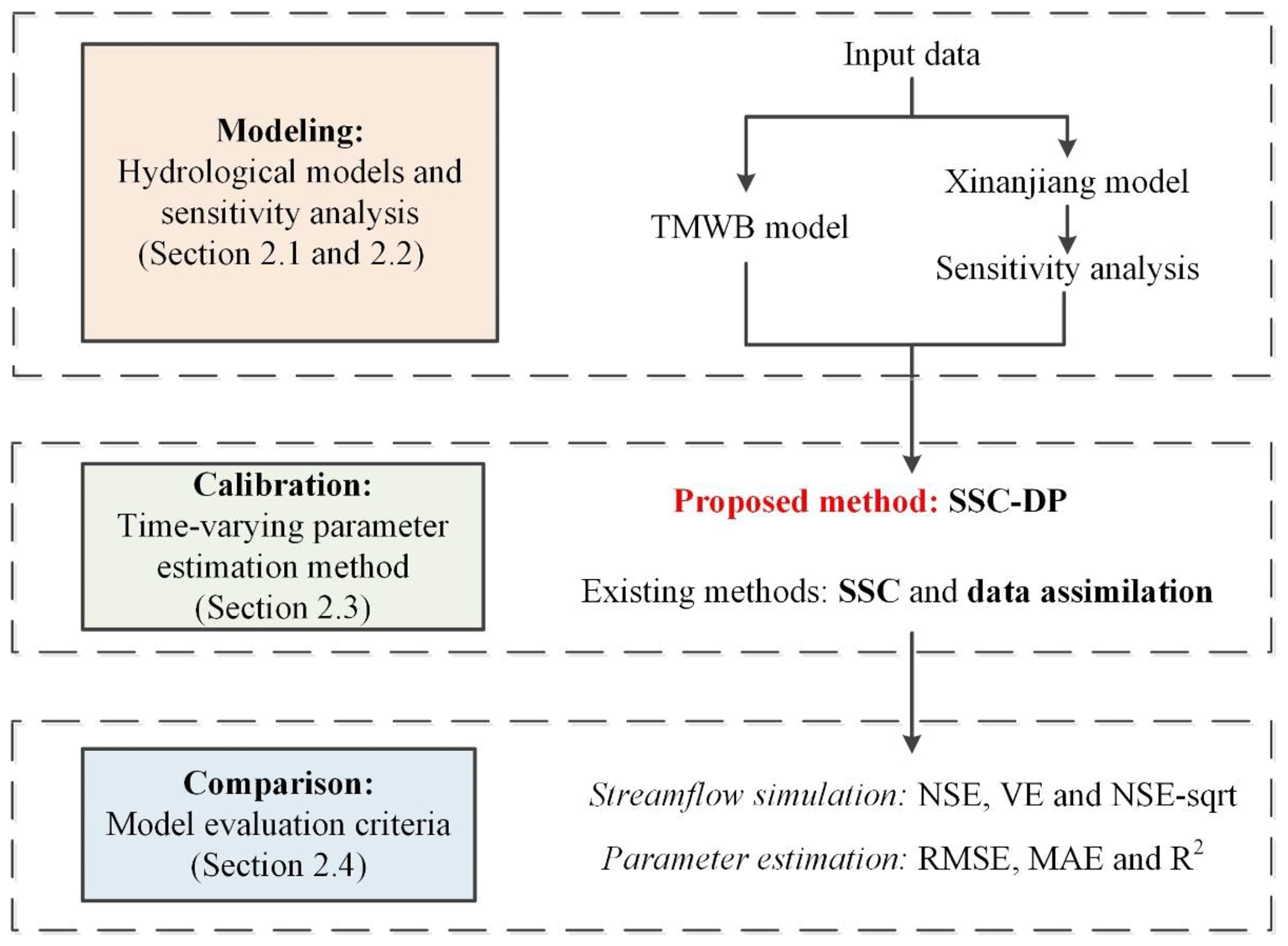
In this section, a SSC-DP method is proposed to identify the time-varying parameters of hydrological models. The two hydrological models considered in this study are the TMWB and Xinanjiang models. Their concepts and differences are presented in Sect. 2.1. A sensitivity analysis is employed to focus efforts on parameters important to calibration and avoid prohibitive computational cost, as outlined in Sect. 2.2. Three time-varying parameter estimation methods (SSC, SSC-DP, and data assimilation) are presented in Sect. 2.3. The SSC and data assimilation are provided for comparisons with the SSC-DP. Finally, to evaluate the performance of the time-varying parameter estimation methods, six evaluation criteria are selected and formulated in Sect. 2.4. The flow chart of the methodologies is shown in Fig. 1.
2.1 Hydrological models
2.1.1 Two-parameter monthly water balance model
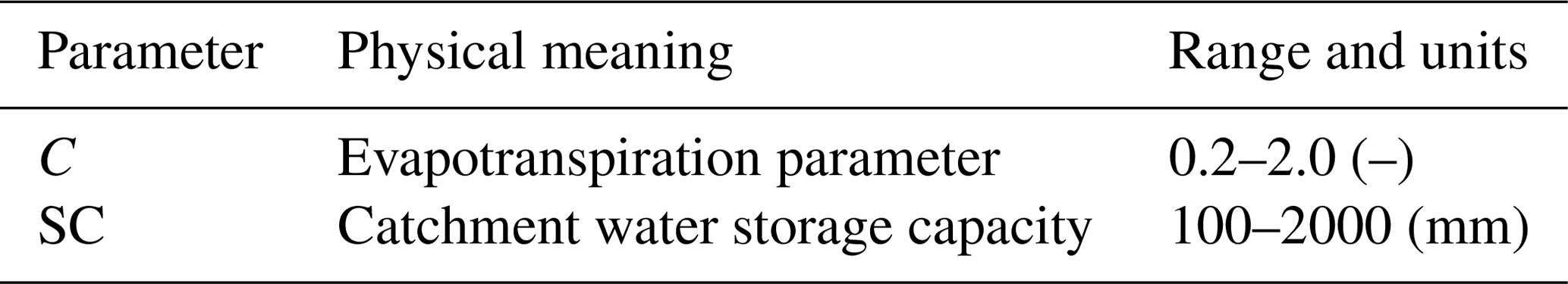
The TMWB model developed by Xiong and Guo (1999) is efficient for monthly runoff simulations and forecasts (Kim et al., 2016; Dai et al., 2018; Yang et al., 2017; Guo et al., 2002). The model requires monthly precipitation and potential evapotranspiration as inputs. Its simplicity and efficiency of performance mean that TMWB can easily be used to investigate the impacts of climate change (Deng et al., 2016; Luo et al., 2019). Its outputs include monthly streamflow, actual evapotranspiration, and the soil moisture content index. The model has only two parameters (Table 1), C and SC. The parameter C takes account of the effect of the change of timescale when simulating actual evapotranspiration. The parameter SC represents the field capacity (mm).

2.1.2 Xinanjiang model
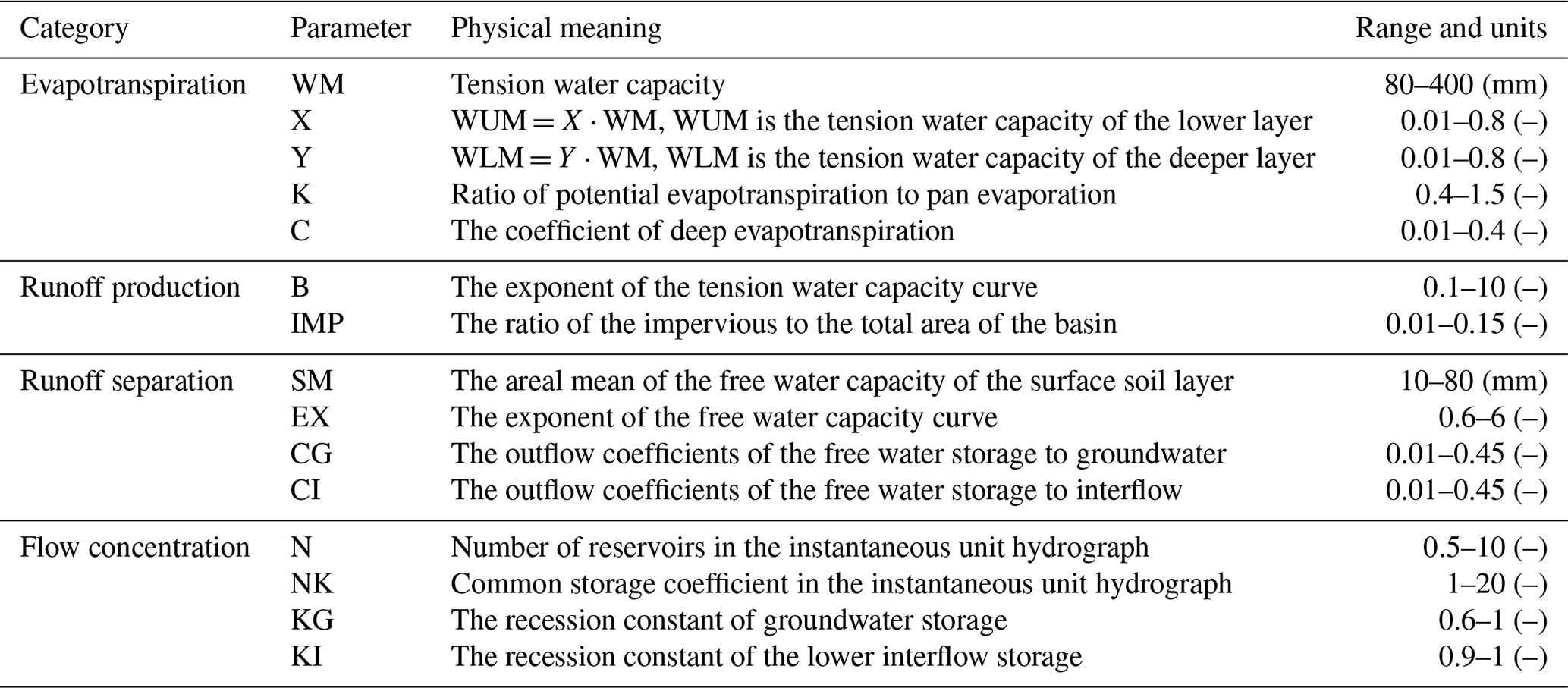
The Xinanjiang model (Zhao, 1992) is widely used in China (Yin et al., 2018; Si et al., 2015; Li and Zhang, 2017). It takes precipitation and pan-evaporation data as inputs and estimates the actual evapotranspiration, soil moisture storage, surface runoff, interflow, and groundwater runoff from the watershed. The simulated streamflow is calculated by summing the routing results of the surface, interflow, and groundwater runoff (Sun et al., 2018). In this study, the surface runoff is routed by the instantaneous unit hydrograph (Lin et al., 2014), while the interflow and groundwater runoff are routed by the linear reservoir method (Jayawardena and Zhou, 2000). A schematic overview of the model is presented in Fig. 2. The meaning, range, and units of all the parameters in the Xinanjiang model are listed in Table 2.
There are two important differences between the TMWB and Xinanjiang models: (1) the TMWB model has two parameters, while the Xinanjiang model has 15 parameters; (2) TMWB is a monthly rainfall–runoff model, whereas the Xinanjiang model can run on hourly or daily step sizes.
2.2 Parameter sensitivity analysis method
Sensitivity analysis is used to identify which parameters significantly affect the performance of the Xinanjiang model and reduce the number of parameters to be calibrated. Numerous sensitivity analysis methods are available, such as the Morris method (Morris, 1991) and Sobol analysis (Sobol, 1993). The Morris method provides similar results to Sobol analysis with a reduced computational burden (Rebolho et al., 2018; Teweldebrhan et al., 2018; Yang et al., 2018).
The Morris method assumes that if parameters change by the same relative amount, the parameter that causes the larger elementary effect is the more sensitive (King and Perera, 2013). The elementary effect is calculated as follows:
where θp represents the pth parameter, Δ is the relative amount, Np is the total number of parameters, and y is the model output based on a particular parameter set.
Each parameter is changed in turn and every parameter set produces an elementary effect. The parameter sensitivity is evaluated using the mean value μ of the elementary effects. If a parameter has a higher value of μ, it is more sensitive. In fact, interactions between parameters should be taken into account (Jie et al., 2018). Hence, the SD σ can be calculated. A higher value of σ indicates a stronger nonlinear correlation between parameters (Pappenberger et al., 2008).
2.3 Time-varying parameter estimation method
2.3.1 Split-sample calibration
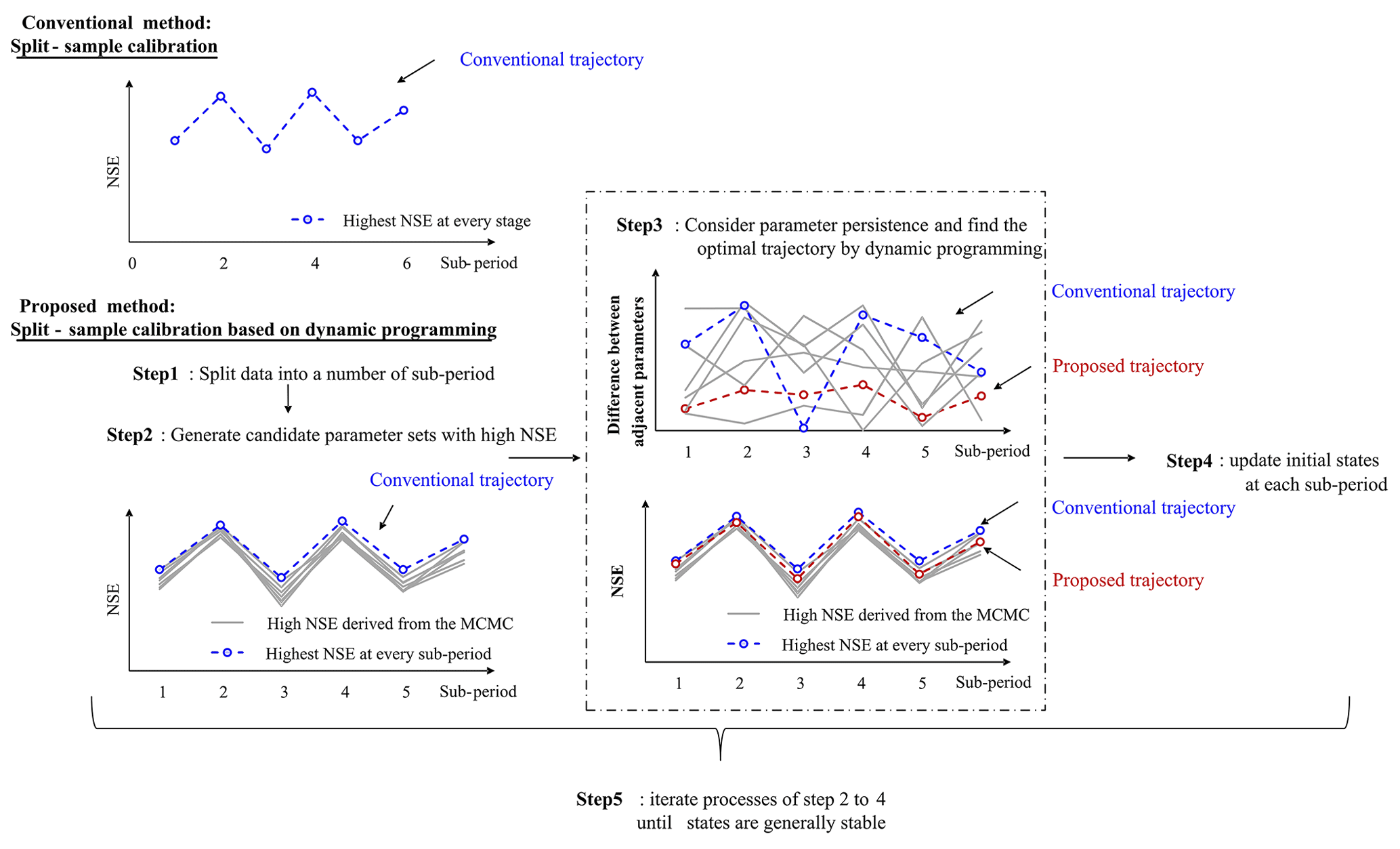
SSC provides a simple way of diagnosing parameter non-stationarity under a changing environment (Merz et al., 2011). As illustrated in Fig. 3a, the method usually has two steps (Kim et al., 2015; Hughes, 2015): (1) available data are divided into several consecutive periods, which can be arbitrarily chosen as hours, days, months, seasons, or years; (2) parameters are calibrated separately for the respective period. This procedure gives better simulation performance than using constant parameters but leads to the estimated parameters fluctuating strongly over adjacent sub-periods, producing false temporal variants.
2.3.2 Split-sample calibration based on dynamic programming
To overcome this problem, the SSC-DP method identifies time-varying parameters with consideration of temporal continuity. SSC-DP has five steps (Fig. 3b):
- 1.
Split the sample periods. This process is the same as the first step of the SSC.
- 2.
Generate an ensemble of near-optimal parameters. Multiple parameter sets with objective values close to the optimum for each sub-period are obtained using Markov chain–Monte Carlo (MCMC) sampling (Chib and Greenberg, 1995). The likelihood measure of the ith sub-period links the parameter to observations using the Nash–Sutcliffe efficiency (NSE) (Nash and Sutcliffe, 1970) as follows:
where Qt and are the observed and simulated runoff at time step t, respectively, and l is the length of the sub-period.
- 3.
Optimize by using dynamic programming. The goal is to find parameters that provide both accurate streamflow simulations and continuity. The continuity condition aims to minimize the difference between the estimated parameters for sub-periods i and i+1. For N sub-periods, the objective function can be expressed as follows:
where θi,p is the pth estimated parameter over the ith sub-period; and are its maximum and minimum values, respectively; NP is the number of the parameters; and α is the weight, reflecting parameter continuity. The weights of NSEi, NSEln ,i, and NSEabs,i are set to 1 following the work of Merz et al. (2011), who used equal weights for the NSE and its variants.
As the decision-making process during the current sub-period is related to that of the previous sub-period, the parameter estimation over N periods becomes a multi-stage optimization problem. To solve this, a dynamic programming technique (Bellman, 1957) is employed to decompose the optimization into a number of single-stage problems and determine the optimal trajectory of the time-varying parameters. Dynamic programming is a useful method for handling sequential operation decisions. It allows the problem to be solved using a backward recursive procedure, whereby the decision-making for each sub-period maximizes the sum of current and future benefits (Ming et al., 2017; Li et al., 2018). In this study, the objective function is formulated as the following recursive equation:
where is the evaluation index using the optimal time-varying parameters from the Nth to the ith sub-periods, and Eq. (6) calculates the objective function from the Nth sub-period to the first sub-period.
- 4.
Update initial states. The initial states, such as that of the soil water content, are important in model simulation and calibration. As the final states for sub-period i are not used as the initial states for sub-period i+1 during steps (1)–(3), the time-varying parameter set obtained from step (3) is applied to the hydrological model to update the initial states of each sub-period for the next iteration.
- 5.
Repeat steps (1)–(4). Steps (1)–(4) are repeated until the initial states of each sub-period are generally stable.
2.3.3 Data assimilation
Another approach for diagnosing variations in parameters is data assimilation, using methods such as the EnKF and ensemble Kalman smoother (EnKS). These are used here as reference methods. The EnKF has been widely applied to conceptual models, including TMWB (Deng et al., 2016). Li et al. (2013) noted that the EnKF struggles to handle the time-lag in routing processes. However, the routing component is vital to the Xinanjiang model. EnKS can efficiently determine the states of the Xinanjiang model (Meng et al., 2017), but the estimation of routing parameters deserves discussion. Most previous studies have used a fixed distribution of the routing hydrograph in data assimilation (Lu et al., 2013); i.e. the parameters are constant for routing processes. With respect to these issues, a modified EnKF (named SSC-EnKF) is established as a third data assimilation reference method in the synthetic experiment with the Xinanjiang model (described in Sect. 3.1).
The EnKF includes two main steps: model prediction and assimilation. The state vector is augmented with parameter variables so that time-varying parameters can be estimated simultaneously with model states. For model prediction, the augmented vector is derived by adding noise on that from the previous time step through the following equation:
where ϑt is the parameter vector at time step t, represented as (); xt is the state vector; and are the kth ensemble member forecasts at time step t+1; and are the updated values of the kth ensemble member forecasts at time step t; ut+1 denotes the forcing data (e.g. precipitation) at time step t+1; and and are the white noise for the kth ensemble member, which follow a Gaussian distribution with zero mean and specified covariance of Rt and Gt, respectively.
In the assimilation process, the augmented vector is updated using the following equations if suitable observations are available:
where yt+1 is the observation vector at time t+1; is the kth observation ensemble member at time step t+1; is the simulation vector at time t+1; h is the observational operator that converts the model states to observations; is the measurement error, which follows a Gaussian distribution with a covariance of Wt; and is the Kalman gain matrix (for details, see Feng et al., 2017).
The EnKS is based on the EnKF. Whereas the EnKF updates the model states and parameters at the current time step, the EnKS takes account of those values over the past time steps. The main steps of the EnKS are identical to those of the EnKF, but the equation of the assimilation process is formulated as follows:
where is the Kalman gain matrix of EnKS. The fixed time window n of EnKS is pre-determined based on the response function or unit hydrograph. Meng et al. (2017) suggested that the time window should be set as half of the recession time of a flood.
A third data assimilation approach is constructed based on the SSC. Instead of assimilating one observed variable, it assimilates the observed variables during a given period in one assimilation process. Assuming that the parameters are constant in the given period, the equation of the assimilation process for the ith sub-period is expressed as follows:
where ϑi is the parameter vector for sub-period i, represented as (); xi is the initial state vector for sub-period i; and l is the length of the sub-period.
This approach addresses the routing-lag issue by allowing parameters of the routing processes, such as the instantaneous unit hydrograph, to remain constant for each sub-period and to be time-varying over the whole period.
2.4 Model evaluation criteria
The streamflow simulations given by the proposed method are verified using the NSE, relative error (RE), and NSE on logarithm of streamflow (NSEln) (Hock, 1999). RE evaluates the error of the total volume of streamflow, while NSE and NSEln evaluate the agreement between the hydrograph of observations and simulations. NSE is more sensitive to high flows, but NSEln focuses more on low flows. Higher values of NSE, and NSEln and lower absolute values of RE indicate better streamflow simulations. The NSE, RE, and NSEln are expressed as followed:
The estimated parameters are evaluated by the RMSE (Alvisi et al., 2006), MARE (Khalil et al., 2001), and R2 (Kim et al., 2007) in the synthetic experiments (see details in Sect. 3.1). RMSE is more sensitive to high values than MARE, while R2 is based on the linear assumption (Dawson et al., 2007). Smaller values of RMSE and MARE and higher values of R2 indicate stronger parameter identification ability. For the pth parameter, the formulations are as follows:
where θt and are the true parameter and its estimated value at the tth time step, respectively; and are the mean value of the true parameters and its estimated values, respectively; and m is the length of the data during the whole period.
Table 3Different cases of synthetic experiments and real catchment case studies for comparison and evaluation.
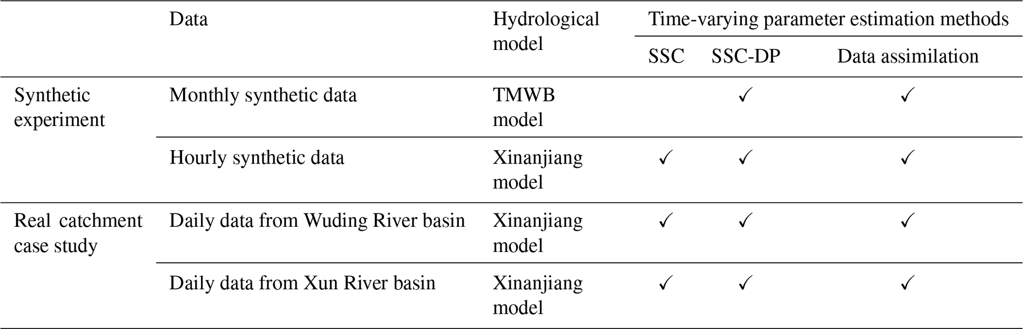
Two synthetic experiments and two real catchment case studies were designed to assess the performance of SSC-DP. The experiments are described in Table 3.
3.1 Synthetic experiments
The two synthetic experiments examine the ability of SSC-DP to identify the time-varying parameters of the TMWB and Xinanjiang hydrological models. The merit of synthetic experiments is that the parameters can be synthetically generated to be either constant or time-varying. Hence, it is convenient to compare the estimated values with the pre-determined parameters to evaluate different parameter estimation methods. Note that synthetic experiments have been successfully used in several time-varying parameter identification studies (Deng et al., 2016; Pathiraja et al., 2016; Xiong et al., 2019).
3.1.1 Synthetic experiment with the TMWB model
Synthetic data of monthly precipitation and potential evapotranspiration were collected from the 03451500 catchment of the Model Parameter Estimation Experiment (MOPEX) (Duan et al., 2006). The data cover 252 months. Runoff was derived by the TMWB model using synthetic precipitation, potential evapotranspiration, and the pre-determined parameters. Gaussian noise was added to the simulated runoff to represent uncertainties. The mean of the noise was set to zero, and the SD was assumed to be 3 % of the magnitude of the values (Deng et al., 2016).
Table 4True parameters of different scenarios in the synthetic experiment with the TMWB model.
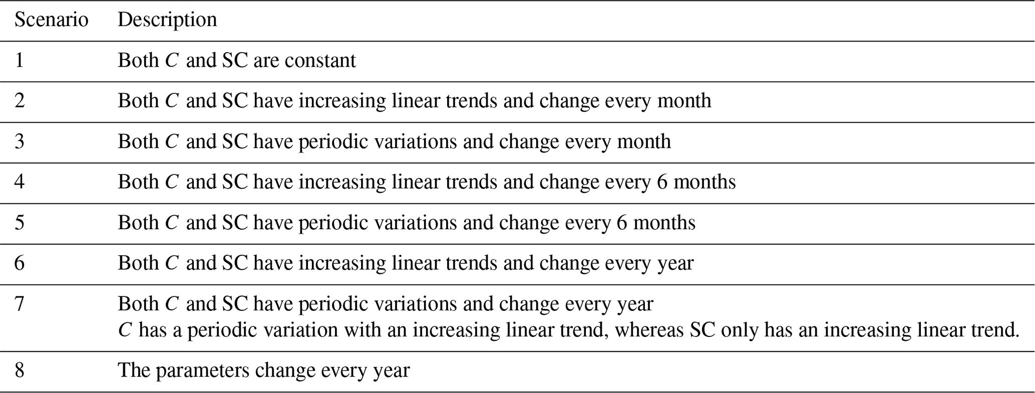
Eight scenarios with different pre-determined parameters were investigated (Table 4). The first scenario considered constant parameters. Scenarios 2 and 3 considered month-by-month variations in TMWB model parameters; i.e. the parameters remain constant during each month but change from month to month. Scenarios 4 and 5 considered parameters that change every 6 months. Scenarios 6–8 considered year-by-year variations. The changes in both C and SC were considered to be linear in scenarios 2, 4, and 6 (trend) and sinusoidal in scenarios 3, 5, and 7 (periodicity), reflecting the impacts of climate change and human activities (Pathiraja et al., 2016). Scenario 8 considered a periodic variation with an increasing trend for parameter C and only the linear variation in SC.
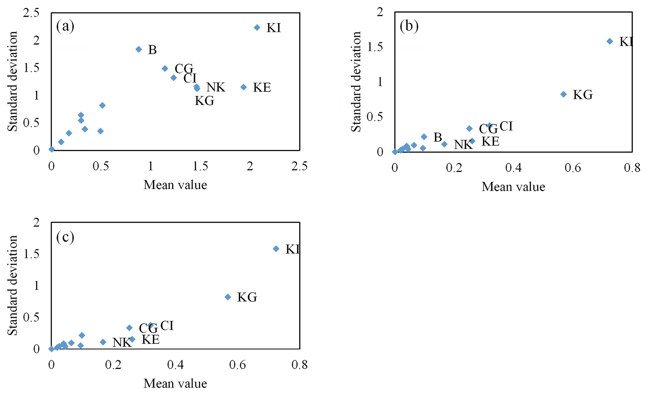
Figure 4Results of the Morris method for the synthetic experiment with the Xinanjiang model. The sensitivity analysis is based on three different kinds of model responses: (a) NSE, (b) NSEabs, (c) NSEln. Only the most sensitive parameters are labelled.
3.1.2 Synthetic experiment with the Xinanjiang model
Hourly precipitation and pan evaporation data were collected from the Baiyunshan Reservoir basin in China. The data cover a period of 18 000 h. The Xinanjiang model has 15 parameters, which can lead to a significant computational burden. To reduce the total number of model runs, only the sensitive parameters were considered to be free. The Morris method was used to detect the free parameters (Fig. 4), with the results showing that KE, CI, CG, KI, KG, and NK are sensitive parameters. Thus, the other parameters were held constant for the whole period.
Table 5True parameters of different scenarios in the synthetic experiment with the Xinanjiang model
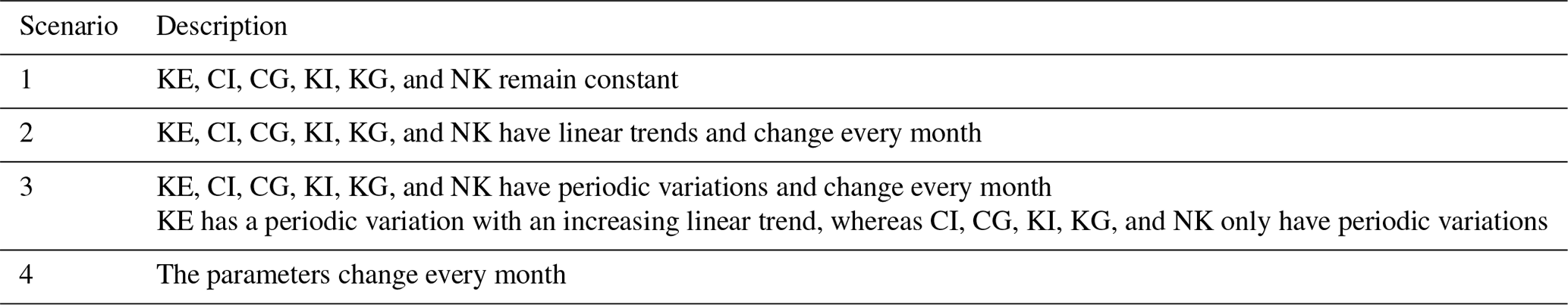
Similar to the experiment with the TMWB model, the synthetic runoff was derived from the Xinanjiang model with added Gaussian noise. The mean of the noise was set to zero, and the SD was assumed to be 5 % of the magnitude of the values. As presented in Table 5, all 15 parameters were set to be constant in the first scenario. The pre-determined sensitive parameters were considered to vary with a certain trend and periodicity in scenarios 2 and 3, respectively. Scenario 4 considered a combined variation of trend and periodicity for the parameter KE, with the other free parameters set to vary linearly. The parameter variations in scenarios 2–4 were assumed to occur once a month.
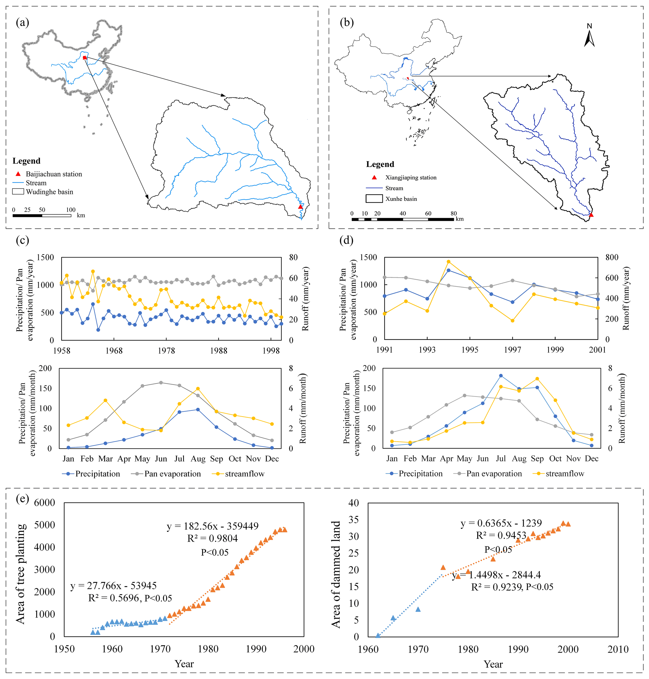
Figure 5Location of (a) Wuding River basin and (b) Xun River basin. The plots (c) and (d) show the average yearly and monthly variations of precipitation, pan evaporation, and streamflow in the Wuding River basin and Xun River basin, respectively. The plot (e) shows the temporal variations in the soil and water conservation measures undertaken in the Wuding River basin.
3.2 Study area: Wuding River basin
The Wuding River basin (Fig. 5a) examined in the first case study is a large sub-basin of the Yellow River basin located on the Loess Plateau (Xu, 2011). The Wuding River has a drainage area of 30 261 km2 and a total length of 491 km. The average slope is 0.2 %, and the elevation varies from 600–1800 . The area is a semi-arid region with mean annual precipitation of ∼ 401 mm. The annual potential evapotranspiration is 1077 mm, and the mean annual runoff is 39 mm. The data for this basin were collected over the period 1958–2000. The daily precipitation was obtained from Thiessen polygons using records from 122 rain gauges. Based on meteorological data from the China Meteorological Data Sharing Service System (http://data.cma.cn, last access: 12 February 2018), areal pan evaporation data were obtained. As illustrated in Fig. 5a, the station furthest downstream, Baijiachuan, drains an area of 29 662 km2 (98 % of the total basin) and records the daily runoff data. The data of the daily precipitation and streamflow in the Wuding River basin were obtained from the local Hydrology and Water Resources Bureau of China, the quality of which has been checked by the official authorities, and there are no gaps among these data for all the hydrological stations. It can be seen from Fig. 5c that the annual streamflow in the Wudinghe River basin has a distinct decreasing trend, while seasonal variations are not significant, but the annual precipitation and pan evaporation generally have no trend, suggesting the impacts of human activities on rainfall–runoff relationships.
Soil and water conservation measures, such as the construction of the check dams and afforestation, have been undertaken since the 1960s. The areas of two soil and water conservation measures are plotted in Fig. 5e, the data of which were collected from Zhang et al. (2002). The areas of tree planting have an increasing trend, but the slope gets much larger after 1972. It indicates that greater efforts have been made for afforestation since the turning point. Similarly, the areas of dammed lands also increase, but the rate gets slower after 1972. These two soil and water conservation measures had changed the underlying surface of the watershed and impacted the relationship between precipitation and runoff (Jiao et al., 2017; Gao et al., 2017).
3.3 Study area: Xun River basin
The proposed method was also applied to the Xun River basin, China (Fig. 5b). Located between 108∘24′–109∘26′ E and 32∘52′–33∘55′ N, the study area covers approximately 6448 km2. The Xun River is ∼ 218 km long and has an average annual flow of 73 m3 s−1 (Li et al., 2016). The basin has a subtropical monsoon climate. The weather is wet and moderate with an annual average temperature of 15–17 ∘C. The daily hydrological data from 1991–2001 include precipitation from 28 rainfall stations, pan evaporation from three hydrological gauged stations, and discharge at the outlet of the Xun River basin. Areal precipitation was obtained using the Thiessen polygon method, and areal pan evaporation was computed using the average value of the data from gauged stations. The data in the Xun River basin were also obtained from the local Hydrology and Water Resources Bureau of China, and there are no gaps among these data for all the hydrological stations.
It can be observed from Fig. 5d that no trend is found in annual precipitation, pan evaporation, and streamflow, suggesting that the relationship between precipitation and runoff of the Xun River basin is rarely affected by human activities during 1991–2001. However, strong seasonal patterns are exhibited in these three climatic and hydrological variables, suggesting that seasonal variations in hydrological parameters should be considered.
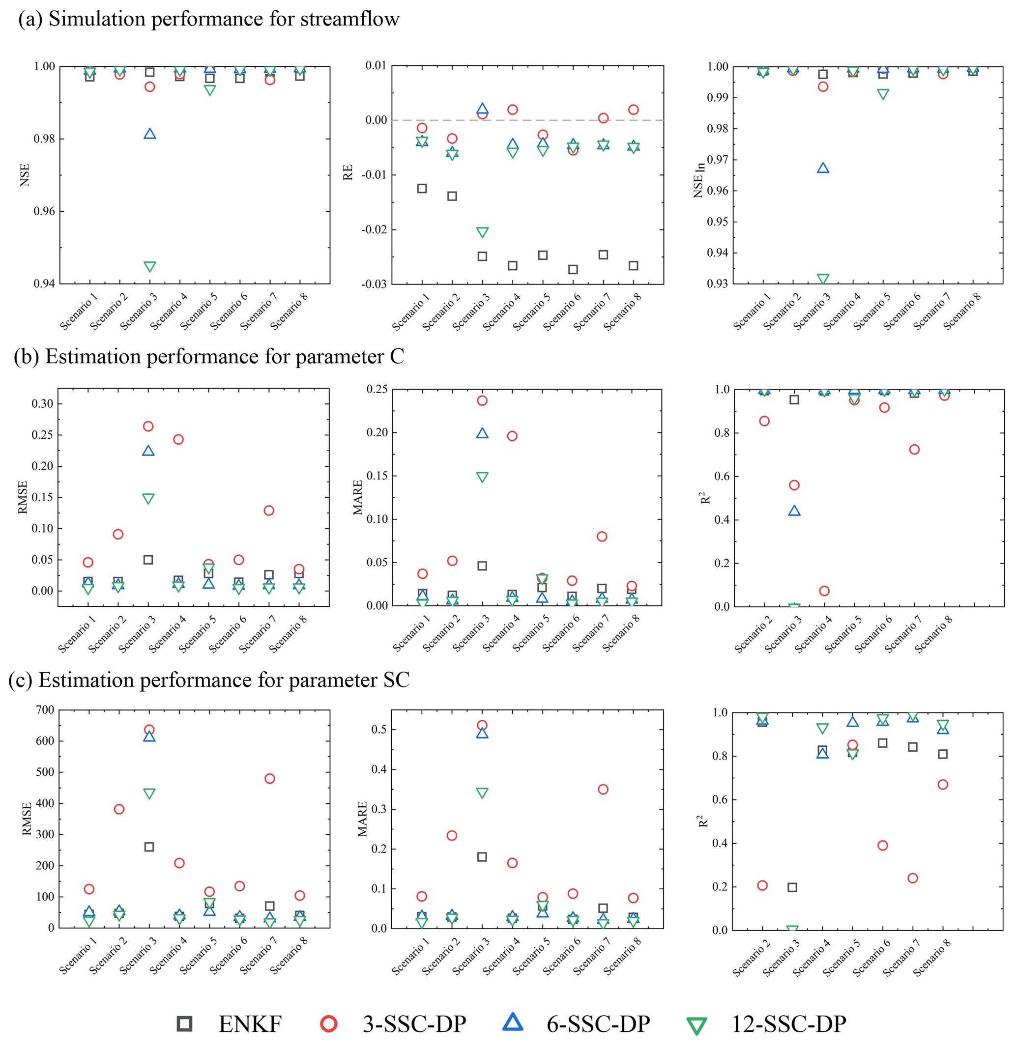
Figure 6Comparison between the EnKF and SSC-DP methods for (a) streamflow simulation and identification of (b) parameter C and (c) parameter SC.
4.1 Synthetic experiment
4.1.1 Results of synthetic experiment with the TMWB model
When using SSC-DP, the first task is to define how the hydrological data series should be split into the k sub-periods within which the parameters are assumed to be constant. As climate change can induce seasonal or half-annual variations while human activities usually influence the watershed annually, lengths of 3 months, 6 months, and 12 months were arbitrarily chosen. Thus, this experiment compared the following four methods: (1) EnKF, (2) 3-SSC-DP, (3) 6-SSC-DP, and (4) 12-SSC-DP.
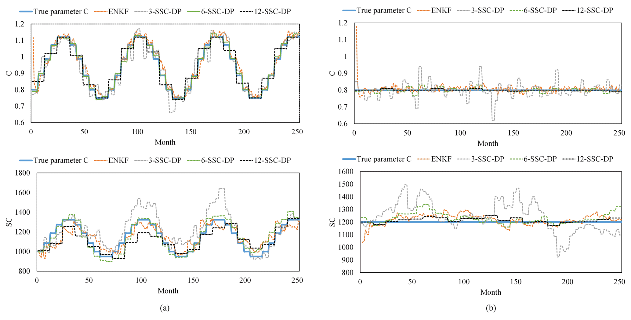
Figure 7Comparison among different methods for (a) scenario 5 and (b) scenario 1 of the synthetic experiment with the TMWB model.
Figure 6a presents the runoff simulation performance for various scenarios. In scenario 1, the NSE values of the three SSC-DP methods are all higher than that of EnKF. The results of NSEln show no significant differences among various methods. For scenarios 2, 4, and 6, where true parameters have linear trends, the 6-SSC-DP and 12-SSC-DP are superior to the EnKF and 3-SSC-DP in terms of NSE and NSEln. In scenario3, where the true parameters have periodic variations and change every month, the NSE and NSEln values of 6-SSC-DP and 12-SSC-DP decrease significantly, because the assumed sub-period length is longer than the timescale of actual variations. Similarly, in scenario 5, 12-SSC-DP performs worst for NSE and NSEln, but 6-SSC-DP performs best. In scenario 7 and 8, both 6-SSC-DP and 12-SSC-DP perform better than EnKF. According to the evaluations of NSE and NSEln, the SSC-DP offers improved accuracy compared to the EnKF if the proper length is chosen. Another advantage of the SSC-DP is the small RE. For all scenarios, the SSC-DP methods significantly outperform for RE compared with EnKF. Among the SSC-DP methods, the RE of 3-SSC-DP is the smallest.
Figure 6b and c focuses on the ability of the four methods to identify time-varying parameters. It can be seen that the RMSE and MARE values of the 3-SSC-DP are larger than those of other methods in most cases. That is because the sub-period length that serves as a calibration period for MCMC is so short (i.e. 3 months) that the estimated parameters are associated with higher uncertainties.
Regarding the synthetic true parameters having constant values (scenario 1), 12-SSC-DP gives the best performance with the lowest RMSE and MARE and highest R2. The observations and estimated parameters are presented in Fig. 7b. It shows that the estimated parameters obtained by EnKF vary at every time step, resulting in larger deviations from the observations than 6-SSC-DP and 12-SSC-DP.
When the synthetic true parameters vary linearly (scenarios 2, 4, and 6), 12-SSC-DP produces the best estimations in comparison with EnKF, 3-SSC-DP, and 6-SSC-DP. The performances of 6-SSC-DP and EnKF are similar.
When the synthetic true parameters vary sinusoidally from month to month, EnKF gives the best estimations in scenario 3. The poor performances of 6-SSC-DP and 12-SSC-DP can be explained by the sub-period length being much longer than the actual one. When the parameters vary periodically at 6-month intervals (scenario 5), 6-SSC-DP yields the best performance with the lowest RMSE and MARE and highest R2. The differences in estimation performances among 3-SSC-DP, 12-SSC-DP, and EnKF are small. The estimated parameters for scenario 5 have been plotted in Fig. 7a. Although 3-SSC-DP and 12-SSC-DP have different lengths of sub-periods, they can also detect the correct seasonal signal of the parameters. For the annual variation in parameters (scenario 7), 12-SSC-DP and 6-SSC-DP produce better results than EnKF. Similar results can be seen in scenario 8, where C has a combined variation from year to year. In summary, the results indicate that the SSC-DP with a suitable length can estimate more accurate parameters than EnKF.
4.1.2 Results of synthetic experiment with the Xinanjiang model
The Xinanjiang model is more complex than TMWB, and so some sensitivity analysis is necessary. As stated in Sect. 3.1.2, the sensitive parameters are KE, CI, CG, KI, KG, and NK. The 18 000 hourly hydrological data points were divided into 25 sub-periods (monthly timescale) and 12 sub-periods (bimonthly timescale). It is considered that a monthly timescale helps diagnose seasonal variations, whereas a 2-month timescale provides data for longer calibration lengths.
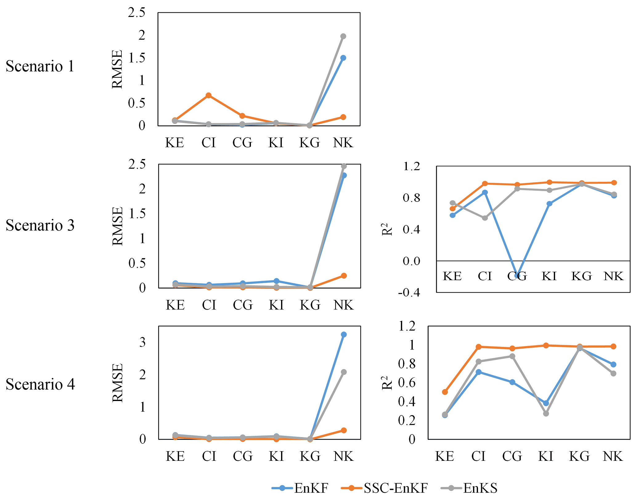
Figure 8Comparison among EnKF, SSC-EnKF, and EnKS in the synthetic experiment with the Xinanjiang model.
Three data assimilation methods (see Sect. 2.3.2 for details) were applied to the synthetic data: (1) EnKF, (2) EnKS, and (3) SSC-EnKF. The results in Fig. 8 indicate that EnKS is superior to EnKF, as previously observed (Li et al., 2013), although SSC-EnKF gives the best results. This is probably because SSC-EnKF is based on the assumption that the parameters remain constant during each sub-period.
The simulated streamflow and identification of time-varying parameters were compared across four methods: 1-SSC, SSC-EnKF, 1-SSC-DP, and 2-SSC-DP. The simulation performance is summarized in Fig. 9a. For all scenarios, the NSE of 2-SSC-DP is the lowest, but it performs better for low flows. The SSC-EnKF produces the highest RE in scenarios 2, 3, and 4, indicating the problem of simulating water balance. The SSC and 1-SSC-DP perform well for all scenarios in terms of NSE, RE, and NSEln. However, the SSC performs better than the 1-SSC-DP with regard to RE, while 1-SSC-DP is slightly superior to SSC in scenario 3 with higher NSEln.

Figure 9Comparison among the SSC, SSC-EnKF, and SSC-DP methods in the synthetic experiment with the Xinanjiang model for (a) streamflow simulation and parameter identification in terms of (b) RMSE, (c) MARE, and (d) R2.
Figure 9b and c compares the time-varying parameter estimation performance among the four methods. In scenarios 1 and 2, 2-SSC-DP produces the lowest RMSE, MARE, and R2, followed by the 1-SSC-DP. The 1-SSC-DP is slightly superior to the 1-SSC and significantly outperforms the SSC-EnKF for the two scenarios.
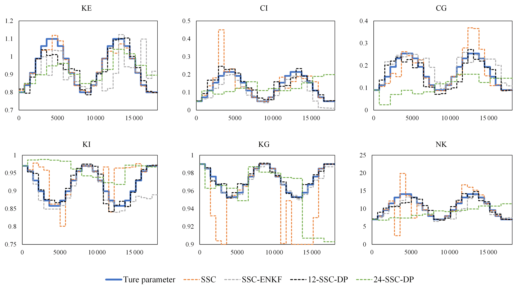
Figure 10Comparison between estimated parameters and their true values for scenario 3 of the synthetic experiment with the Xinanjiang model.
When the synthetic true parameters vary sinusoidally from month to month (scenario 3), the estimated parameters are plotted in Fig. 10. It can be seen that 1-SSC-DP successfully detects a seasonal signal in every parameter. The SSC-EnKF performs well for R2, but it has high MARE. Although the average MARE values of the SSC and 2-SSC-DP are lower than those of SSC-EnKF, their R2 are relatively low. From Fig. 10, the estimated parameters by the 1-SSC generally fluctuate periodically, but the variations are dramatic, resulting in the lowest R2 for CI, KI, KG, and NK. The estimated parameters of the 2-SSC-DP fluctuate more slowly, but the sub-period length is too long. In scenario 4, 1-SSC performs better than the SSC-EnKF and 2-SSC-DP but is still slightly inferior to the 1-SSC-DP. Overall, the 1-SSC-DP achieves higher-quality and more robust parameter estimations performances than the other methods.
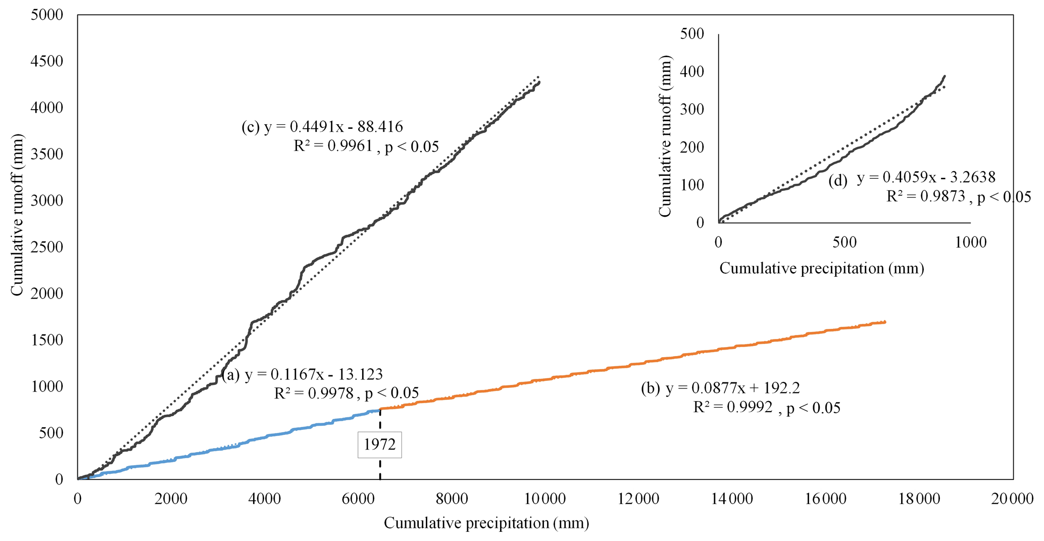
Figure 11Double mass curves between daily runoff and precipitation for (a) Wuding River basin from 1958–1972; (b) Wuding River basin from 1973–2000; (c) Xun River basin from 1991–2001. Subgraph (d) represents the double mass curve between the mean daily runoff and precipitation from 1991–2001.
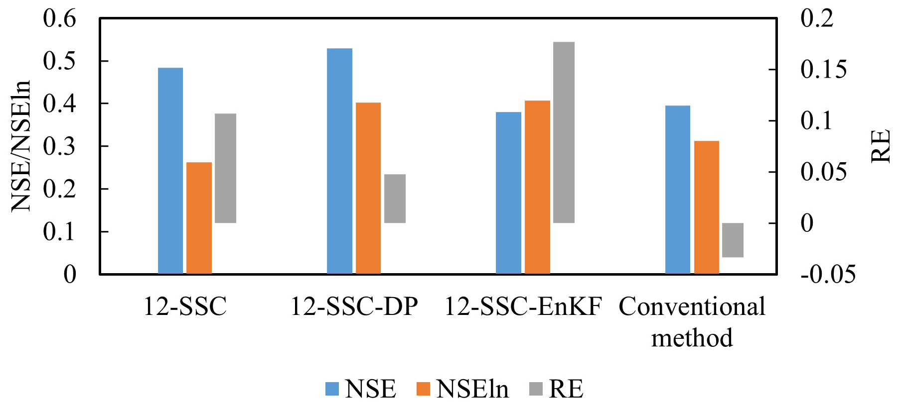
Figure 12Simulation performance for streamflow in the Wuding River basin. The results of NSE and NSEln are shown on the primary axis, while the values of RE are shown on the secondary axis.
4.2 Case study: Wuding River basin
Figure 11a and b show the double mass curves between daily runoff and precipitation for the Wuding River basin. Similar to the work of Deng et al. (2016), the two linear slopes (p value < 0.05) of the curves are different before and after 1972, demonstrating the relationship between precipitation and runoff changes under the soil and water conservation measures. This suggests that there are annual variations in the watershed characteristics. Hence, the length of each sub-period was set to 12 months, and the time-varying parameters were identified using 12-SSC-DP. Based on daily Wuding data from 1958–2000, sensitivity analysis showed that nine parameters of the Xinanjiang model are relatively sensitive: WM, WUM, WLM, KE, IMP, KI, KG, N, and NK.
The simulation results given by 12-SSC-DP were benchmarked against those from 12-SSC, data assimilation, and the conventional method in which all Xinanjiang model parameters remain constant. The simulation performance is presented in Fig. 12. The values of the NSEs are relatively low, because the streamflow in dry regions is difficult to simulate. It can be seen that the 12-SSC-DP gives the best simulation results among different methods with the highest NSE and NSEln and small RE. Although the 12-SSC produces relatively high NSE, it performs the worst simulations for low flows. The SSC-EnKF has relatively high NSEln, but its RE is the largest. Overall, the 12-SSC-DP significantly improves the simulation performance of the Xinanjiang model in the Wuding River basin.
Although the objective function of 12-SSC-DP considers the trade-off between simulation accuracy and parameter continuity, 12-SSC-DP gives a higher NSE value. This may be because 12-SSC locates a local peak over one sub-period, resulting in unreasonable model states for the beginning of the next sub-period, whereas 12-SSC-DP uses dynamic programming to explore more reasonable parameter values and model states. Figure 13 shows the quantile–quantile plots, from which it can be seen that if the parameters are assumed to be constant, streamflow is highly underestimated. The underestimation mainly derives from the deficiencies of the model structure. Methods 12-SSC and 12-SSC-DP reduce this underestimation by using time-varying parameters. Additionally, 12-SSC-DP is slightly inferior to 12-SSC in terms of peak flows but is superior in terms of simulating streamflow lower than 100 m3 s−1, which accounts for 80 % of the whole streamflow time series. It can be inferred that the 12-SSC-DP is more applicable to the simulation of streamflow in the Wuding River basin.
The estimated time-varying parameters estimated by 12-SSC-DP are plotted in Fig. 14. The results show that WM remains constant before and after 1972, but WUM varies significantly over this period, indicating that the distribution of soil water capacity may change, i.e. WUM decreases but WLM increases. A Person correlation analysis is applied to investigate the relationship between the areas of tree planting and WUM as well as WLM. It is found that there is a significant negative correlation (Pearson correlation efficient ρ = −0.38, P<0.05) between the areas of tree planting and WUM, while WLM has a non-significant positive correlation (ρ = 0.26, P>0.05) with the areas of tree planting. It can be inferred that less severe soil erosion occurred, because the upper layers became thinner while the lower layer, where vegetation roots dominate, became thicker (Jayawardena and Zhou, 2000). Additionally, IMP is significantly correlated with the areas of tree planting (ρ = −0.33, P<0.05). Except for afforestation, the areas of the dammed lands are significantly correlated with WLM (ρ = 0.46, P<0.05), suggesting that the construction of the check dams also has an influence on the soil water capacity of the Wuding river basin. Other parameters, KE, KI, KG, N, and NK, show little difference before and after 1972. The variations in WLM and IMP slowed down after the turning point, similar to the results of Deng et al. (2016).
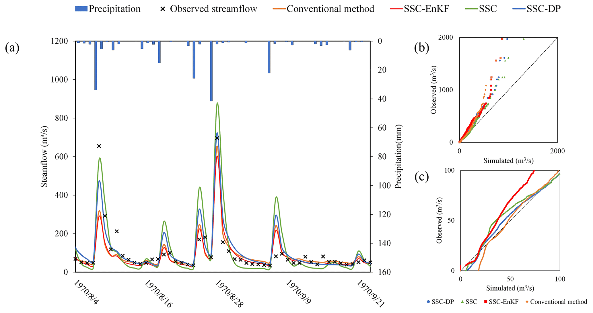
Figure 13The simulated and observed streamflow using the conventional method, SSC-EnKF, SSC, and SSC-DP for the Wuding River basin. (a) Streamflow simulation hydrograph. (b) The quantile–quantile plot for all streamflow. (c) The quantile–quantile plot for streamflow lower than 100 m3 s−1.
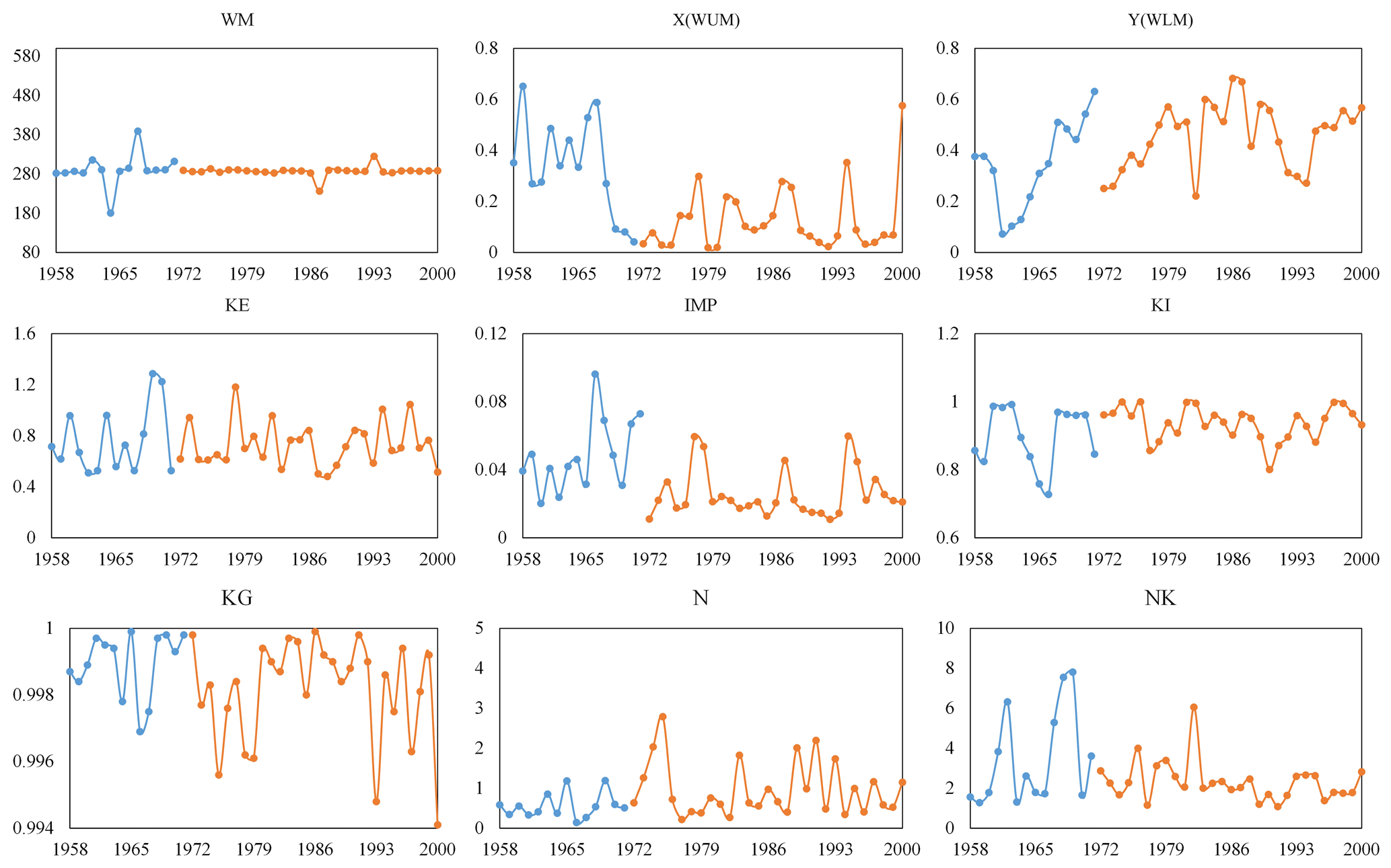
Figure 14Estimated sensitive parameters of the Xinanjiang model for the Wuding River basin. The blue and orange solid lines represent the estimated parameters pre- and post-1972, respectively.
4.3 Case study: Xun River basin
Figure 11c and d show the double mass curves between runoff and precipitation for the Xun River basin. The linear slope of the curve is generally stationary for the whole 10-year period shown in Fig. 11c, with a correlation coefficient of 99.6 %. In contrast, the linear slope for an intra-annual timescale is non-stationary (Fig. 11d). Based on these results, it can be inferred that the relationship between precipitation and runoff is stable from 1990–2000 but varies over the intra-annual timescale. Hence, sub-periods of 3 and 12 months were examined in the Xun River basin using models 3-SSC-DP and 12-SSC-DP. From the Xun River basin data from 1991–2000, sensitivity analysis suggested that five parameters of the Xinanjiang model are relatively sensitive, namely KE, B, KI, KG, and NK.

Figure 15Simulation performance for streamflow in the Xun River basin. The results of NSE and NSEln are shown on the primary axis, while the values of RE are shown on the secondary axis.
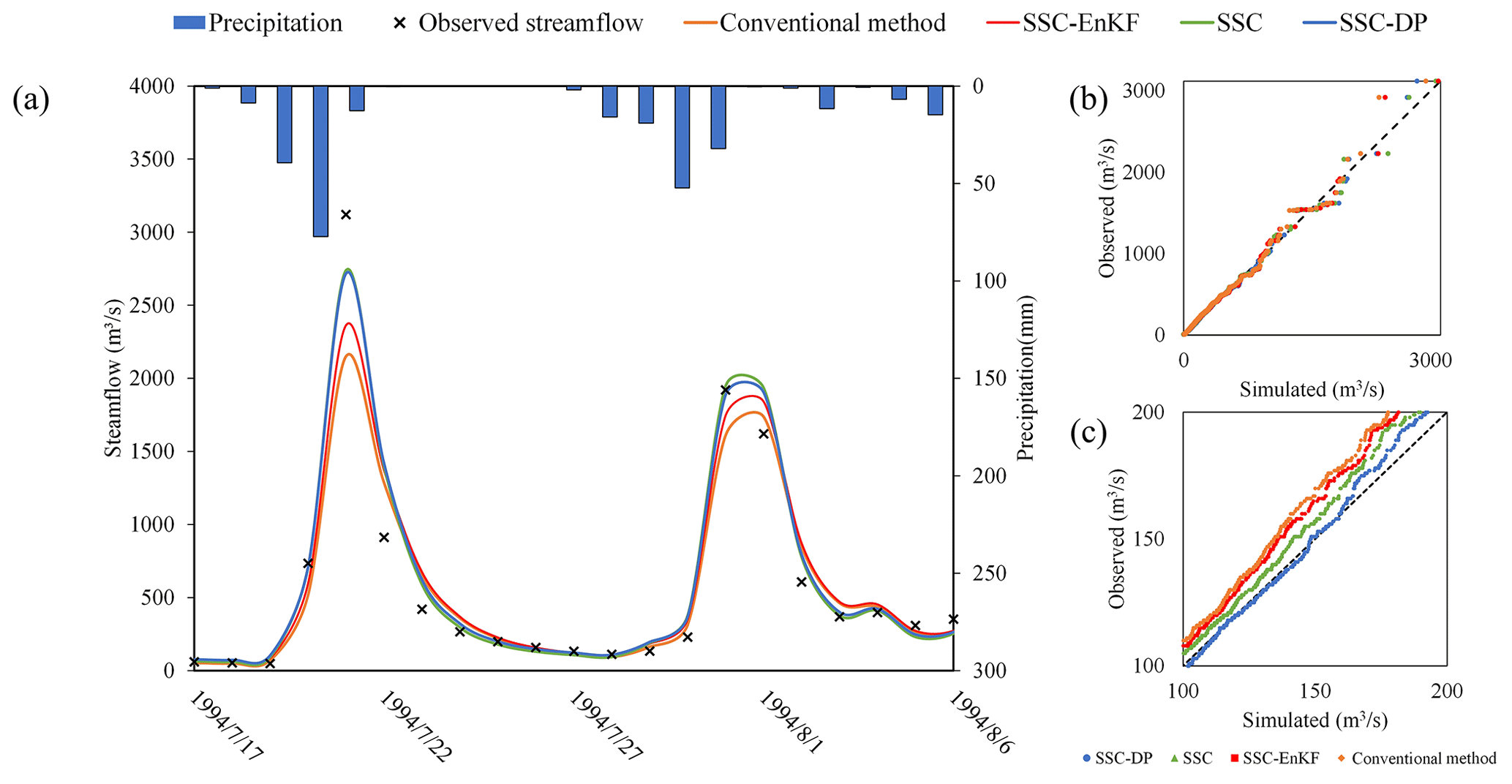
Figure 16The simulated and observed streamflow using the conventional method, SSC-EnKF, SSC, and SSC-DP for the Xun River basin. (a) Streamflow simulation hydrograph. (b) The quantile–quantile plot for all streamflow. (c) The quantile–quantile plot for streamflow ranging from 100 to 200 m3 s−1.
Similar to the case study of the Wuding River basin, the simulation performance of 3-SSC-DP was benchmarked against that of 3-SSC, data assimilation, and the conventional calibration method. Among the data assimilation methods described in Sect. 2.3.2, 3-SSC-EnKF gives the highest simulation accuracy. The simulation performance is presented in Fig. 15. All methods performed well, with NSE values of 92.5 %, 93.0 %, 95.0 %, and 94.8 % for the conventional method, 3-SSC-EnKF, 3-SSC, and 3-SSC-DP, respectively. 3-SSC and 3-SSC-DP also perform well for NSEln compared with 3-SSC-EnKF and the conventional method. However, with regard to RE, the values are 0.0007 and 0.0324 for 3-SSC-DP and 3-SSC-DP, respectively. This indicated that the 3-SSC-DP can better simulate water balance than the 3-SSC in the Xun River basin. Figure 16 illustrates the hydrograph and quantile–quantile plots for the simulations in the Xun river basin. It is evident that the peak flows estimated by the 3-SSC are higher than those of 3-SSC-DP, and 3-SSC-DP simulates better the flows ranging from 100 to 200 m3 s−1.
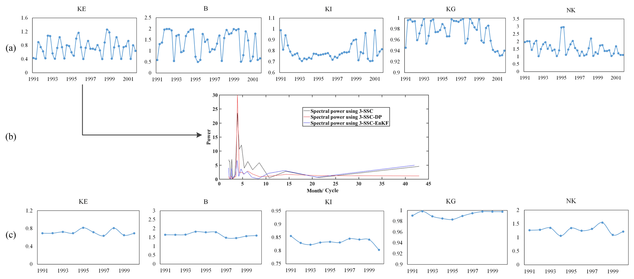
Figure 17Estimated sensitive parameters of the Xinanjiang model for the Xun River basin over (a) a seasonal timescale and (c) an annual timescale. Plot (b) illustrates the spectral power of parameter KE using different methods.
The estimated parameters using 3-SSC-DP are presented in Fig. 17a. Some parameters vary significantly over an intra-annual timescale. Among them, the parameter KE, representing the ratio of potential evapotranspiration to pan evaporation, exhibits the most distinct seasonal variations. A fast Fourier transform was used to calculate the spectral power of the KE time series to explore its periodic characteristics. As can be observed from Fig. 17b, 3-SSC-DP had the greatest spectral power, for a period of 4.0 cycles per year, somewhat higher than the power obtained by 3-SSC and 3-SSC-EnKF. This means a stronger periodic pattern is captured by 12-SSC-DP. Given that the estimated KE varies at 3-month intervals, it has a 1-year periodicity. The other parameters do not exhibit significant 1-year periodic patterns. This may be because only KE, linking potential evapotranspiration and pan evaporation, is directly impacted by seasonal climate variations, such as temperature.
As noted in the methodology section, the performance of the proposed method is influenced by several factors, such as the weights in the objective function and the choice of lengths. Some suggestions regarding the improvement of the proposed approach are now discussed in detail.
5.1 Objective function of dynamic programming in SSC-DP
In the conventional method, a parameter set is identified as optimal for providing the best simulation over the calibration period. However, other parameter sets with slightly worse (but still good) performance can also be candidates. Allowing for input data uncertainty and local optima, SSC-DP identifies parameter sets that perform near-optimally and display fewer fluctuations over sub-periods. This can be adjusted by weights in the objective function of the dynamic programming approach (see Eq. 3). As the weighting for accuracy increases, parameters providing more accurate simulations are chosen, but parameter continuity is less important. If too much importance is given to continuity, the variations in real-world processes may be underestimated. Here, the influence of different weights has been assessed for simulation accuracy and parameter continuity based on synthetic experiments with the TMWB and Xinanjiang models, respectively. Specifically, the weight for simulation accuracy was set to 1, and the weight for parameter continuity α varied from zero to a small positive value (e.g. 1). When α=0, only simulation accuracy was considered.
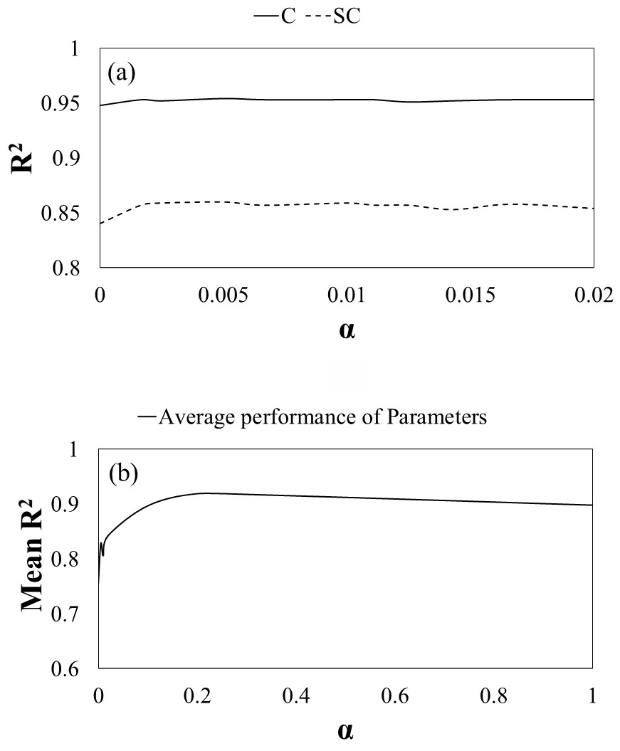
Figure 18Correlation efficiency results of SSC-DP using different weights of parameter continuity for synthetic experiments with (a) the TMWB model and (b) the Xinanjiang model. The mean R2 is the average value of the R2 such that the identification results for parameters with different ranges can be summarized.
Figure 18a shows the R2 value of 12-SSC-DP with various continuity weights for scenario 4 in the synthetic experiment with the TMWB model. It can be seen that R2 is lowest when α=0 for both C and SC. There is some improvement when a nonzero weight is applied. As α increases, the performance of 12-SSC-DP improves and then worsens; the differences among schemes with nonzero weights are not distinct. Similar results can be observed in Fig. 18b, which presents the R2 value of 12-SSC-DP with various α values for scenario 2 in the synthetic experiment with the Xinanjiang model. Therefore, nonzero continuity weights can significantly improve the parameter estimation performance compared with the zero-weight case. It is suggested that weights of 1 (accuracy) and 0.005 (continuity) be used with the TMWB model and weights of 1 (accuracy) and 0.2 (continuity) be applied with the Xinanjiang model, as in this study.
5.2 Choice of sub-period length in SSC-DP
As mentioned by Gharari et al. (2013), there are different ways of determining the sub-period lengths. The sub-periods can be non-continuous hydrological years (Seiller et al., 2012), months or seasons (Deng et al., 2018; Paik et al., 2005), and discharge or precipitation events (Singh and Bardossy, 2012). This introduces a controversial issue whereby parameters are impacted by the length of the calibration period. Merz et al. (2009) suggested that 3–5 years is an acceptable calibration period, whereas Singh and Bardossy (2012) indicated that a small number of events may be sufficient for parameter identification. It is suggested that the determination of the sub-period length considers three factors:
- 1.
The temporal scale of climate change or human activities. For example, the Wudinghe River basin is taken as a case study. The soil and water conservation measures have led to long-term change in the catchment characteristic since the 1960s. Due to this, the yearly sub-period is preferred.
- 2.
The seasonality. Contrary to the Wudinghe River basin, the relationship between precipitation and runoff of the Xun River basin is rarely affected by human activities during 1991–2001. However, its significant seasonal dynamics can be observed and has been studied in the literature (Lan et al., 2020, 2018). In order to diagnose the seasonality, the stable period of 3 months is adopted.
- 3.
The simulation accuracy. The length should be neither too long nor too short so as to increase the reliability of the calibration while guaranteeing that variations in real processes are captured. Thus, given that the timescale of the variations is unknown, the proposed SSC-DP can be used with different split-sample lengths. It is suggested that the length should be as long as possible without degrading the simulation performance significantly. For example, in the synthetic experiment with the TMWB model, if the difference between the NSE values of 6-SSC-DP and 3-SSC-DP is small, the preferred length is 6 months.
However, many studies are based on the conventional assumption that the parameters of different sub-periods are independent. Hence, the sub-period lengths should be long enough to reduce the degree of uncertainty. In this study, the assumption of parameter continuity is introduced to give another constraint that considers correlations between parameters of adjacent sub-periods. It appears that the determination of sub-period lengths deserves further investigation.
This paper has described a time-varying parameter estimation approach based on dynamic programming. The proposed SSC-DP combines the basic concept of SSC and the continuity assumption of data assimilation to estimate more continuous parameters while providing comparably good streamflow simulations. Two synthetic experiments were designed to evaluate its applicability and efficiency for time-varying parameter identification. Furthermore, two case studies were conducted to explore the advantages of SSC-DP in real catchments. From the results, the following conclusions can be drawn:
- 1.
The proposed method with a suitable length not only produces better simulation performance, but also ensures more accurate parameter estimates than SSC and EnKF in the synthetic experiment using the TMWB model with two parameters. The impact of sub-period lengths on the performance of SSC-DP is significant when the pre-determined parameters vary sinusoidally.
- 2.
The proposed method can be used to deal with complex hydrological models involving a large number of parameters, demonstrated by the synthetic experiment using the Xinanjiang model with 15 parameters. A sensitivity analysis was performed to reduce the probable computational cost and improve the efficiency of identifying the time-varying parameters.
- 3.
The proposed method has the potential to detect the relationship between the time-varying parameters and dynamic catchment characteristics. For example, SSC-DP produces the best simulation performance in the case study of the Wuding River basin and detects that parameters representing soil water capacity and impervious areas changed significantly after 1972, reflecting the soil and water conservation projects carried out from 1958–2000. Additionally, SSC-DP detects the strongest seasonal signal in the case study of Xun River basin, indicating the distinct impacts of seasonal climate variability.
This study has demonstrated that the proposed method is an effective approach for identifying time-varying parameters under changing environments. Further work is still needed, such as to determine an objective method for choosing the sub-period lengths.
The data and code that support the findings of this study are available from the corresponding author upon request.
All of the authors helped to develop the method, designed the experiments, analysed the results, and wrote the paper.
The authors declare that they have no conflict of interest.
This study was supported by the Innovation Team in Key Field of the Ministry of Science and Technology (2018RA4014), the National Natural Science Foundation of China (51861125102), and Natural Science Foundation of Hubei Province (2017CFA015). The authors would like to thank the editor and anonymous reviewers for their comments that helped improve the quality of the paper.
This research has been supported by the Innovation Team in Key Field of the Ministry of Science and Technology (grant no. 2018RA4014) and the National Natural Science Foundation of China (grant no. 51861125102).
This paper was edited by Dimitri Solomatine and reviewed by two anonymous referees.
Alvisi, S., Mascellani, G., Franchini, M., and Bárdossy, A.: Water level forecasting through fuzzy logic and artificial neural network approaches, Hydrol. Earth Syst. Sci., 10, 1–17, https://doi.org/10.5194/hess-10-1-2006, 2006.
Bellman, R.: Dynamic programming, Princeton University Press, Princeton, 1957.
Broderick, C., Matthews, T., Wilby, R. L., Bastola, S., and Murphy, C.: Transferability of hydrological models and ensemble averaging methods between contrasting climatic periods, Water Resour. Res., 52, 8343–8373, https://doi.org/10.1002/2016wr018850, 2016.
Bronstert, A.: Rainfall-runoff modelling for assessing impacts of climate and land-use change, Hydrol. Process., 18, 567–570, https://doi.org/10.1002/hyp.5500, 2004.
Chen, Y. and Zhang, D.: Data assimilation for transient flow in geologic formations via ensemble Kalman filter, Adv. Water Resour., 29, 1107–1122, https://doi.org/10.1016/j.advwatres.2005.09.007, 2006.
Chib, S. and Greenberg, E.: Understanding the Metropolis-Hastings algorithm, Am. Stat., 49, 327–335, https://doi.org/10.2307/2684568, 1995.
Coron, L., Andreassian, V., Perrin, C., Lerat, J., Vaze, J., Bourqui, M., and Hendrickx, F.: Crash testing hydrological models in contrasted climate conditions: An experiment on 216 Australian catchments, Water Resour. Res., 48, https://doi.org/10.1029/2011wr011721, 2012.
Dai, C., Qin, X. S., Chen, Y., and Guo, H. C.: Dealing with equality and benefit for water allocation in a lake watershed: A Gini-coefficient based stochastic optimization approach, J. Hydrol., 561, 322–334, https://doi.org/10.1016/j.jhydrol.2018.04.012, 2018.
Dawson, C. W., Abrahart, R. J., and See, L. M.: HydroTest: A web-based toolbox of evaluation metrics for the standardised assessment of hydrological forecasts, Environ. Model. Softw., 22, 1034–1052, https://doi.org/10.1016/j.envsoft.2006.06.008, 2007.
Deng, C., Liu, P., Guo, S., Li, Z., and Wang, D.: Identification of hydrological model parameter variation using ensemble Kalman filter, Hydrol. Earth Syst. Sci., 20, 4949–4961, https://doi.org/10.5194/hess-20-4949-2016, 2016.
Deng, C., Liu, P., Wang, D., and Wang, W.: Temporal variation and scaling of parameters for a monthly hydrologic model, J. Hydrol., 558, 290–300, https://doi.org/10.1016/j.jhydrol.2018.01.049, 2018.
Deng, C., Liu, P., Wang, W., Shao, Q., and Wang, D.: Modelling time-variant parameters of a two-parameter monthly water balance model, J. Hydrol., 573, 918–936, https://doi.org/10.1016/j.jhydrol.2019.04.027, 2019.
Duan, Q., Schaake, J., Andreassian, V., Franks, S., Goteti, G., Gupta, H. V., Gusev, Y. M., Habets, F., Hall, A., Hay, L., Hogue, T., Huang, M., Leavesley, G., Liang, X., Nasonova, O. N., Noilhan, J., Oudin, L., Sorooshian, S., Wagener, T., and Wood, E. F.: Model Parameter Estimation Experiment (MOPEX): An overview of science strategy and major results from the second and third workshops, J. Hydrol., 320, 3–17, https://doi.org/10.1016/j.jhydrol.2005.07.031, 2006.
Feng, M., Liu, P., Guo, S., Shi, L., Deng, C., and Ming, B.: Deriving adaptive operating rules of hydropower reservoirs using time-varying parameters generated by the EnKF, Water Resour. Res., 53, 6885–6907, https://doi.org/10.1002/2016wr020180, 2017.
Fowler, K., Peel, M., Western, A., and Zhang, L.: Improved rainfall-runoff calibration for drying climate: Choice of objective function, Water Resour. Res., 54, 3392–3408, https://doi.org/10.1029/2017wr022466, 2018.
Fowler, K. J. A., Peel, M. C., Western, A. W., Zhang, L., and Peterson, T. J.: Simulating runoff under changing climatic conditions: Revisiting an apparent deficiency of conceptual rainfall-runoff models, Water Resour. Res., 52, 1820–1846, https://doi.org/10.1002/2015wr018068, 2016.
Gao, S., Liu, P., Pan, Z., Ming, B., Guo, S., and Xiong, L.: Derivation of low flow frequency distributions under human activities and its implications, J. Hydrol., 549, 294–300, https://doi.org/10.1016/j.jhydrol.2017.03.071, 2017.
Gharari, S., Hrachowitz, M., Fenicia, F., and Savenije, H. H. G.: An approach to identify time consistent model parameters: sub-period calibration, Hydrol. Earth Syst. Sci., 17, 149–161, https://doi.org/10.5194/hess-17-149-2013, 2013.
Guo, S. L., Wang, J. X., Xiong, L. H., Ying, A. W., and Li, D. F.: A macro-scale and semi-distributed monthly water balance model to predict climate change impacts in China, J. Hydrol., 268, 1–15, https://doi.org/10.1016/s0022-1694(02)00075-6, 2002.
Guzha, A. C., Rufino, M. C., Okoth, S., Jacobs, S., and Nobrega, R. L. B.: Impacts of land use and land cover change on surface runoff, discharge and low flows: Evidence from East Africa, J. Hydrol.: Reg. Stud., 15, 49–67, https://doi.org/10.1016/j.ejrh.2017.11.005, 2018.
Hock, R.: A distributed temperature-index ice- and snowmelt model including potential direct solar radiation, J. Glaciol., 45, 101–111, https://doi.org/10.3189/s0022143000003087, 1999.
Hughes, D. A.: Simulating temporal variability in catchment response using a monthly rainfall-runoff model, Hydrolog. Sci. J., 60, 1286–1298, https://doi.org/10.1080/02626667.2014.909598, 2015.
Hundecha, Y. and Bardossy, A.: Modeling of the effect of land use changes on the runoff generation of a river basin through parameter regionalization of a watershed model, J. Hydrol., 292, 281–295, https://doi.org/10.1016/j.jhydrol.2004.01.002, 2004.
Jayawardena, A. W. and Zhou, M. C.: A modified spatial soil moisture storage capacity distribution curve for the Xinanjiang model, J. Hydrol., 227, 93–113, https://doi.org/10.1016/s0022-1694(99)00173-0, 2000.
Jeremiah, E., Marshall, L., Sisson, S. A., and Sharma, A.: Specifying a hierarchical mixture of experts for hydrologic modeling: Gating function variable selection, Water Resour. Res., 49, 2926–2939, https://doi.org/10.1002/wrcr.20150, 2013.
Jiao, Y., Lei, H., Yang, D., Huang, M., Liu, D., and Yuan, X.: Impact of vegetation dynamics on hydrological processes in a semi-arid basin by using a land surface-hydrology coupled model, J. Hydrol., 551, 116–131, https://doi.org/10.1016/j.jhydrol.2017.05.060, 2017.
Jie, M. X., Chen, H., Xu, C. Y., Zeng, Q., Chen, J., Kim, J. S., Guo, S. L., and Guo, F. Q.: Transferability of conceptual hydrological models across temporal resolutions: Approach and application, Water Resour. Manage., 32, 1367–1381, https://doi.org/10.1007/s11269-017-1874-4, 2018.
Khalil, M., Panu, U. S., and Lennox, W. C.: Groups and neural networks based streamflow data infilling procedures, J. Hydrol., 241, 153–176, https://doi.org/10.1016/s0022-1694(00)00332-2, 2001.
Kim, S., Hong, S. J., Kang, N., Noh, H. S., and Kim, H. S.: A comparative study on a simple two-parameter monthly water balance model and the Kajiyama formula for monthly runoff estimation, Hydrolog. Sci. J., 61, 1244–1252, https://doi.org/10.1080/02626667.2015.1006228, 2016.
Kim, S. M., Benham, B. L., Brannan, K. M., Zeckoski, R. W., and Doherty, J.: Comparison of hydrologic calibration of HSPF using automatic and manual methods, Water Resour. Res., 43, W01402, https://doi.org/10.1029/2006wr004883, 2007.
Kim, S. S. H., Hughes, J. D., Chen, J., Dutta, D., and Vaze, J.: Determining probability distributions of parameter performances for time-series model calibration: A river system trial, J. Hydrol., 530, 361–371, https://doi.org/10.1016/j.jhydrol.2015.09.073, 2015.
King, D. M. and Perera, B. J. C.: Morris method of sensitivity analysis applied to assess the importance of input variables on urban water supply yield – A case study, J. Hydrol., 477, 17–32, https://doi.org/10.1016/j.jhydrol.2012.10.017, 2013.
Klemes, V.: Operational testing of hydrological simulation-models, Hydrolog. Sci. J., 31, 13–24, https://doi.org/10.1080/02626668609491024, 1986.
Lan, T., Lin, K. R., Liu, Z. Y., He, Y. H., Xu, C. Y., Zhang, H. B., and Chen, X. H.: A clustering preprocessing framework for the subannual calibration of a hydrological model considering climate-land surface variations, Water Resour. Res., 54, 10034–10052, https://doi.org/10.1029/2018WR023160, 2018.
Lan, T., Lin, K., Xu, C.-Y., Tan, X., and Chen, X.: Dynamics of hydrological-model parameters: mechanisms, problems and solutions, Hydrol. Earth Syst. Sci., 24, 1347–1366, https://doi.org/10.5194/hess-24-1347-2020, 2020.
Li, H. and Zhang, Y.: Regionalising rainfall-runoff modelling for predicting daily runoff: Comparing gridded spatial proximity and gridded integrated similarity approaches against their lumped counterparts, J. Hydrol., 550, 279–293, https://doi.org/10.1016/j.jhydrol.2017.05.015, 2017.
Li, H., Liu, P., Guo, S., Ming, B., Cheng, L., and Zhou, Y.: Hybrid two-stage stochastic methods using scenario-based forecasts for reservoir refill operations, J. Water Resour. Plan. Manage., 144, 04018080, https://doi.org/10.1061/(asce)wr.1943-5452.0001013, 2018.
Li, Y., Ryu, D., Western, A. W., and Wang, Q. J.: Assimilation of stream discharge for flood forecasting: The benefits of accounting for routing time lags, Water Resour. Res., 49, 1887–1900, https://doi.org/10.1002/wrcr.20169, 2013.
Li, Z., Liu, P., Deng, C., Guo, S., He, P., and Wang, C.: Evaluation of estimation of distribution algorithm to calibrate computationally intensive hydrologic model, J. Hydrol. Eng., 21, 04016012, https://doi.org/10.1061/(asce)he.1943-5584.0001350, 2016.
Lin, K., Lv, F., Chen, L., Singh, V. P., Zhang, Q., and Chen, X.: Xinanjiang model combined with Curve Number to simulate the effect of land use change on environmental flow, J. Hydrol., 519, 3142–3152, https://doi.org/10.1016/j.jhydrol.2014.10.049, 2014.
Lu, H., Hou, T., Horton, R., Zhu, Y., Chen, X., Jia, Y., Wang, W., and Fu, X.: The streamflow estimation using the Xinanjiang rainfall runoff model and dual state-parameter estimation method, J. Hydrol., 480, 102–114, https://doi.org/10.1016/j.jhydrol.2012.12.011, 2013.
Luo, M., Pan, C., and Zhan, C.: Diagnosis of change in structural characteristics of streamflow series based on selection of complexity measurement methods: Fenhe river basin, China, J. Hydrol. Eng., 24, 05018028, https://doi.org/10.1061/(asce)he.1943-5584.0001748, 2019.
Meng, S., Xie, X., and Liang, S.: Assimilation of soil moisture and streamflow observations to improve flood forecasting with considering runoff routing lags, J. Hydrol., 550, 568–579, https://doi.org/10.1016/j.jhydrol.2017.05.024, 2017.
Merz, R., Parajka, J., and Bloeschl, G.: Scale effects in conceptual hydrological modeling, Water Resour. Res., 45, W09405, https://doi.org/10.1029/2009wr007872, 2009.
Merz, R., Parajka, J., and Bloeschl, G.: Time stability of catchment model parameters: Implications for climate impact analyses, Water Resour. Res., 47, W02531, https://doi.org/10.1029/2010WR009505, 2011.
Ming, B., Liu, P., Bai, T., Tang, R., and Feng, M.: Improving optimization efficiency for reservoir operation using a search space reduction method, Water Resour. Manage., 31, 1173–1190, https://doi.org/10.1007/s11269-017-1569-x, 2017.
Moradkhani, H., Sorooshian, S., Gupta, H. V., and Houser, P. R.: Dual state-parameter estimation of hydrological models using ensemble Kalman filter, Adv. Water Resour., 28, 135–147, https://doi.org/10.1016/j.advwatres.2004.09.002, 2005.
Morris, M. D.: Factorial sampling plans for preliminary computational experiments, Technometrics, 33, 161–174, https://doi.org/10.2307/1269043, 1991.
Nash, J. E. and Sutcliffe, J. V.: River flow forecasting through conceptual models part I – A discussion of principles, J. Hydrol., 10, 282–290, https://doi.org/10.1016/0022-1694(70)90255-6, 1970.
Paik, K., Kim, J. H., Kim, H. S., and Lee, D. R.: A conceptual rainfall-runoff model considering seasonal variation, Hydrol. Process., 19, 3837–3850, https://doi.org/10.1002/hyp.5984, 2005.
Pappenberger, F., Beven, K. J., Ratto, M., and Matgen, P.: Multi-method global sensitivity analysis of flood inundation models, Adv. Water Resour., 31, 1–14, https://doi.org/10.1016/j.advwatres.2007.04.009, 2008.
Pathiraja, S., Marshall, L., Sharma, A., and Moradkhani, H.: Hydrologic modeling in dynamic catchments: A data assimilation approach, Water Resour. Res., 52, 3350–3372, https://doi.org/10.1002/2015wr017192, 2016.
Pathiraja, S., Anghileri, D., Burlando, P., Sharma, A., Marshall, L., and Moradkhani, H.: Time-varying parameter models for catchments with land use change: the importance of model structure, Hydrol. Earth Syst. Sci., 22, 2903–2919, https://doi.org/10.5194/hess-22-2903-2018, 2018.
Poulin, A., Brissette, F., Leconte, R., Arsenault, R., and Malo, J.-S.: Uncertainty of hydrological modelling in climate change impact studies in a Canadian, snow-dominated river basin, J. Hydrol., 409, 626–636, https://doi.org/10.1016/j.jhydrol.2011.08.057, 2011.
Quoc Quan, T., De Niel, J., and Willems, P.: Spatially distributed conceptual hydrological model building: A genetic top-down approach starting from lumped models, Water Resour. Res., 54, 8064–8085, https://doi.org/10.1029/2018wr023566, 2018.
Rebolho, C., Andréassian, V., and Le Moine, N.: Inundation mapping based on reach-scale effective geometry, Hydrol. Earth Syst. Sci., 22, 5967–5985, https://doi.org/10.5194/hess-22-5967-2018, 2018.
Refsgaard, J. C. and Knudsen, J.: Operational validation and intercomparison of different types of hydrological models, Water Resour. Res., 32, 2189–2202, https://doi.org/10.1029/96wr00896, 1996.
Seiller, G., Anctil, F., and Perrin, C.: Multimodel evaluation of twenty lumped hydrological models under contrasted climate conditions, Hydrol. Earth Syst. Sci., 16, 1171–1189, https://doi.org/10.5194/hess-16-1171-2012, 2012.
Si, W., Bao, W., and Gupta, H. V.: Updating real-time flood forecasts via the dynamic system response curve method, Water Resour. Res., 51, 5128–5144, https://doi.org/10.1002/2015wr017234, 2015.
Singh, S. K. and Bardossy, A.: Calibration of hydrological models on hydrologically unusual events, Adv. Water Resour., 38, 81–91, https://doi.org/10.1016/j.advwatres.2011.12.006, 2012.
Siriwardena, L., Finlayson, B. L., and McMahon, T. A.: The impact of land use change on catchment hydrology in large catchments: The Comet River, Central Queensland, Australia, J. Hydrol., 326, 199–214, https://doi.org/10.1016/j.jhydrol.2005.10.030, 2006.
Sobol, I. M.: Sensitivity estimates for nonlinear mathematical models, Math. Model. Comput. Exp., 1, 407–414, 1993.
Stephens, C. M., Marshall, L. A., and Johnson, F. M.: Investigating strategies to improve hydrologic model performance in a changing climate, J. Hydrol., 579, 124219, https://doi.org/10.1016/j.jhydrol.2019.124219, 2019.
Sun, Y., Bao, W., Jiang, P., Ji, X., Gao, S., Xu, Y., Zhang, Q., and Si, W.: Development of multivariable dynamic system response curve method for real-time flood forecasting correction, Water Resour. Res., 54, 4730–4749, https://doi.org/10.1029/2018wr022555, 2018.
Teweldebrhan, A. T., Burkhart, J. F., and Schuler, T. V.: Parameter uncertainty analysis for an operational hydrological model using residual-based and limits of acceptability approaches, Hydrol. Earth Syst. Sci., 22, 5021–5039, https://doi.org/10.5194/hess-22-5021-2018, 2018.
Thirel, G., Andreassian, V., Perrin, C., Audouy, J. N., Berthet, L., Edwards, P., Folton, N., Furusho, C., Kuentz, A., Lerat, J., Lindstrom, G., Martin, E., Mathevet, T., Merz, R., Parajka, J., Ruelland, D., and Vaze, J.: Hydrology under change: an evaluation protocol to investigate how hydrological models deal with changing catchments, Hydrolog. Sci. J., 60, 1184–1199, https://doi.org/10.1080/02626667.2014.967248, 2015.
Toth, E. and Brath, A.: Multistep ahead streamflow forecasting: Role of calibration data in conceptual and neural network modeling, Water Resour. Res., 43, W11405, https://doi.org/10.1029/2006wr005383, 2007.
Westra, S., Thyer, M., Leonard, M., Kavetski, D., and Lambert, M.: A strategy for diagnosing and interpreting hydrological model nonstationarity, Water Resour. Res., 50, 5090–5113, https://doi.org/10.1002/2013wr014719, 2014.
Xie, S., Du, J., Zhou, X., Zhang, X., Feng, X., Zheng, W., Li, Z., and Xu, C.-Y.: A progressive segmented optimization algorithm for calibrating time-variant parameters of the snowmelt runoff model (SRM), J. Hydrol., 566, 470–483, https://doi.org/10.1016/j.jhydrol.2018.09.030, 2018.
Xiong, L. H. and Guo, S. L.: A two-parameter monthly water balance model and its application, J. Hydrol., 216, 111–123, https://doi.org/10.1016/s0022-1694(98)00297-2, 1999.
Xiong, M., Liu, P., Cheng, L., Deng, C., Gui, Z., Zhang, X., and Liu, Y.: Identifying time-varying hydrological model parameters to improve simulation efficiency by the ensemble Kalman filter: A joint assimilation of streamflow and actual evapotranspiration, J. Hydrol., 568, 758–768, https://doi.org/10.1016/j.jhydrol.2018.11.038, 2019.
Xu, J.: Variation in annual runoff of the Wudinghe River as influenced by climate change and human activity, Quatern. Int., 244, 230–237, https://doi.org/10.1016/j.quaint.2010.09.014, 2011.
Yang, N., Zhang, K., Hong, Y., Zhao, Q., Huang, Q., Xu, Y., Xue, X., and Chen, S.: Evaluation of the TRMM multisatellite precipitation analysis and its applicability in supporting reservoir operation and water resources management in Hanjiang basin, China, J. Hydrol., 549, 313–325, https://doi.org/10.1016/j.jhydrol.2017.04.006, 2017.
Yang, X., Jomaa, S., Zink, M., Fleckenstein, J. H., Borchardt, D., and Rode, M.: A new fully distributed model of nitrate transport and removal at catchment scale, Water Resour. Res., 54, 5856–5877, https://doi.org/10.1029/2017wr022380, 2018.
Yin, J., Guo, S., He, S., Guo, J., Hong, X., and Liu, Z.: A copula-based analysis of projected climate changes to bivariate flood quantiles, J. Hydrol., 566, 23–42, https://doi.org/10.1016/j.jhydrol.2018.08.053, 2018.
Zhang, J., Ji, W., and Feng, X.: Water and sediment changes in the Wudinghe River: present state, formative cause and tendency in the future, in: A Study of Water and Sediment Changes in the Yellow River, edited by: Wang, G. and Fan, Z., Publishing House of Yellow River Water Conservancy, Zhengzhou, 393–429, 2002.
Zhao, R. J.: The Xinanjiang model applied in China, J. Hydrol., 135, 371–381, 1992.