the Creative Commons Attribution 4.0 License.
the Creative Commons Attribution 4.0 License.
 | 23 Dec 2021
Effects of aquifer geometry on seawater intrusion in annulus segment island aquifers
Zhaoyang Luo
Chengji Shen
Pei Xin
Chunhui Lu
Ling Li
David Andrew Barry
Seawater intrusion in island aquifers was considered analytically, specifically for annulus segment aquifers (ASAs), i.e., aquifers that (in plan) have the shape of an annulus segment. Based on the Ghijben–Herzberg and hillslope-storage Boussinesq equations, analytical solutions were derived for steady-state seawater intrusion in ASAs, with a focus on the freshwater–seawater interface and its corresponding watertable elevation. Predictions of the analytical solutions compared well with experimental data, and so they were employed to investigate the effects of aquifer geometry on seawater intrusion in island aquifers. Three different ASA geometries were compared: convergent (smaller side is facing the lagoon, larger side is the internal no-flow boundary and flow converges towards the lagoon), rectangular and divergent (smaller side is the internal no-flow boundary, larger side is facing the sea and flow diverges towards the sea). Depending on the aquifer geometry, seawater intrusion was found to vary greatly, such that the assumption of a rectangular aquifer to model an ASA can lead to poor estimates of seawater intrusion. Other factors being equal, compared with rectangular aquifers, seawater intrusion is more extensive, and watertable elevation is lower in divergent aquifers, with the opposite tendency in convergent aquifers. Sensitivity analysis further indicated that the effects of aquifer geometry on seawater intrusion and watertable elevation vary with aquifer width and distance from the circle center to the inner arc (the lagoon boundary for convergent aquifers or the internal no-flow boundary for divergent aquifers). A larger aquifer width and distance from the circle center to the inner arc weaken the effects of aquifer geometry, and hence differences in predictions for the three geometries become less pronounced.
- Article
(4216 KB) - Full-text XML
- BibTeX
- EndNote


Islands are extensively distributed throughout the world's oceans. Unfortunately, their groundwater resources are impacted by sea-level rise and increased demands. According to a recent estimate, there are approximately 65 million people living on oceanic islands where groundwater may be the only source of freshwater (Thomas et al., 2020). Fresh groundwater stored on oceanic islands is mainly from precipitation (usually in the form of a freshwater lens), and its availability varies due to different factors, e.g., island topography, rainfall patterns, tides, episodic storms and human activities (White and Falkland, 2010; Storlazzi et al., 2018). Seawater intrusion is thus an important issue due to its deleterious effect on oceanic island freshwater storage (e.g., Werner et al., 2017; Lu et al., 2019; Memari et al., 2020).
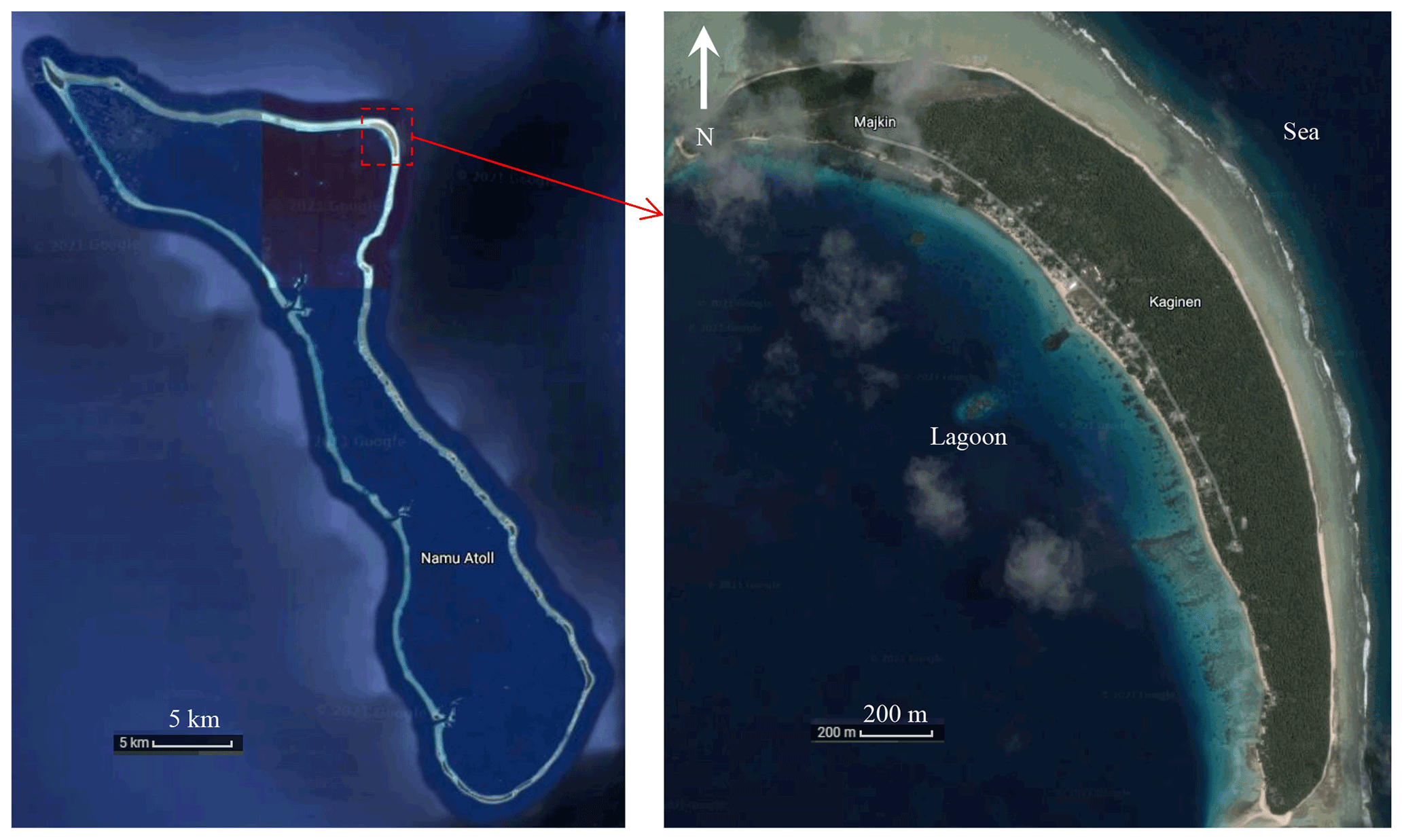
Figure 1Island with an annulus segment in the Namu Atoll, Marshall Islands (© Google Earth 2021).
Over the past few decades, seawater intrusion in oceanic islands has been extensively investigated by field observations (e.g., Röper et al., 2013; Post et al., 2019), laboratory experiments (e.g., Stoeckl et al., 2015; Bedekar et al., 2019; Memari et al., 2020), numerical simulations (e.g., Lam, 1974; Gingerich et al., 2017; Liu and Tokunaga, 2019) and analytical solutions (e.g., Fetter, 1972; Ketabchi et al., 2014; Lu et al., 2019). Among these, analytical solutions are effective tools to assess the extent of seawater intrusion (i.e., the location of the freshwater–seawater interface), although they cannot incorporate complex factors (e.g., dispersive mixing and transient oceanic dynamics) (Werner et al., 2013). The advantages of analytical solutions are that they are computationally efficient, can be used as test cases for numerical models and can reveal the explicit relationships between parameters that influence seawater intrusion (e.g., Fetter, 1972; Ketabchi et al., 2014; Liu et al., 2014; Lu et al., 2019).
Based on the Dupuit–Forchheimer approximation (i.e., ignoring vertical flow) and the Ghijben–Herzberg equation (Drabbe and Badon Ghijben, 1889, English translation given by Post, 2018; Herzberg, 1901), Fetter (1972) presented analytical solutions describing the freshwater–seawater interface location and watertable elevation in a circular island. Bailey et al. (2010) further compared these single-layered analytical solutions with field measurements, indicating that the analytical solutions perform well in estimating the freshwater–seawater interface location and watertable elevation. Fetter's solutions formed the foundation for many subsequent analytical studies on seawater intrusion in island aquifers. Again, for a single layer, Chesnaux and Allen (2008) and Greskowiak et al. (2013) developed analytical solutions to predict the steady-state groundwater age distribution in freshwater lenses. In addition, using single-layered analytical solutions, Morgan and Werner (2014) proposed vulnerability indicators of freshwater lenses under sea-level rise and recharge change.
Since aquifers are usually heterogeneous, the single-layer analytical solutions were subsequently extended to two-layered island aquifers. Vacher (1988) derived solutions for the freshwater–seawater interface location and watertable elevation for infinite-strip islands composed of different layers. Dose et al. (2014) conducted laboratory experiments to validate and confirm the reliability of analytical solutions proposed by Fetter (1972) and Vacher (1988). Ketabchi et al. (2014) extended Fetter's analytical solutions to calculate the freshwater–seawater interface location and watertable elevation in two-layered circular islands subject to sea-level rise. Their results indicated that land-surface inundation caused by sea-level rise has a considerable impact on fresh groundwater lenses. Recently, Lu et al. (2019) derived analytical solutions for the freshwater–seawater interface location and watertable elevation for both strip and circular islands with two adjacent layers, i.e., a less permeable slice along the shoreline of an island and a more permeable zone inland.
All the abovementioned analytical solutions apply to either strip or circular islands. According to the classification of sand dunes developed by Stuyfzand (1993, 2017), there are different island layouts that should be considered, e.g., where the shape of the island is an annulus segment, instead of a strip or circular disk (Fig. 1). Annulus segment-shaped islands are found in various atolls (i.e., circular chains of islands surrounding a central lagoon) as found in the Pacific and Indian oceans (Werner et al., 2017; Duvat, 2019). Nevertheless, analytical solutions of seawater intrusion are not yet available for annulus segment aquifers (ASAs). In general, ASAs are conceptually treated as a 2D cross section, similar to strip islands (e.g., Ayers and Vacher, 1986; Underwood et al., 1992; Bailey et al., 2009; Werner et al., 2017). Evidently, topography plays an important role in groundwater flow and hence seawater intrusion (e.g., Zhang et al., 2016; Liu and Tokunaga, 2019). It remains unclear whether analytical solutions of seawater intrusion for strip islands are appropriate for ASAs. It is also unclear how island geometry affects the freshwater–seawater interface location and watertable elevation of ASAs.
In this study, analytical solutions are derived for steady-state seawater intrusion for ASAs, with a focus on the freshwater–seawater interface location and its corresponding watertable elevation. After comparing their predictions with experimental data (Memari et al., 2020), the analytical solutions are employed to investigate the effects of aquifer geometry on the freshwater–seawater interface location and watertable elevation in ASAs.
Figure 2 shows the conceptual model of an ASA (a slice of an atoll island). The plan view of the model domain is represented as a sector (EFGH) with an angle θ (Fig. 2a). The sea (EF) and lagoon (HG) boundaries are located at L+L0 (L) and L0 (L) from the circle center, respectively. Since the longitudinal length is usually much longer than the lateral length for an atoll island (Werner et al., 2017), seawater intrusion from the lateral sides (EH and FG, Fig. 2a) is negligible in comparison to the longitudinal side, especially for the middle portion of an ASA. Therefore, EH and FG are treated as lateral no-flow boundaries. Note that treating the lateral sides as no-flow boundaries is often used in studies of freshwater lenses on atoll islands (e.g., Ayers and Vacher, 1986; Underwood et al., 1992; Bailey et al., 2009; Werner et al., 2017). The lateral vertical cross section of the model domain is conceptualized as a rectangle (ABCD) along the radial direction with dimensions of L (L) (width) × d (L) (height) (Fig. 2b and c). AD is the impermeable base, while BC is the land surface through which aquifer recharge flows.

Figure 2Conceptual model of an annulus segment aquifer (a slice of an atoll island). (a) Plan view and (b, c) lateral vertical cross section with the saltwater interface tip (b) above the aquifer bed (single location) and (c) on the aquifer bed (two locations). In (a), the sea boundary is on EF, and the atoll lagoon boundary is on HG; in (b) and (c), AD is the impermeable base, and OO* is the internal no-flow boundary.
Both the sea and lagoon water levels are set to Hs (L), which results in an internal no-flow boundary (water divide, where the slope of the watertable is zero) between the sea and lagoon (location of the z axis in Fig. 2b and c). The segment between the sea and the internal no-flow boundary is referred to as Unit 1, whereas the segment between the internal no-flow and lagoon boundaries is referred to as Unit 2 (Fig. 2). The widths of Units 1 and 2 are l1 (L) and l2 (L), respectively. In addition, the flow is asymmetrical in Units 1 and 2, with divergent flow (the aquifer length w (L) increases along the flow direction) in Unit 1 and convergent flow (w decreases along the flow direction) in Unit 2.
The r−z coordinate origin is placed at the intersection of the internal no-flow boundary and impermeable base, with the r axis pointing to the circle center (radial direction) and the z axis pointing vertically upward. Further, ϕ (L) is the watertable height, h (L) is the vertical distance between the watertable and the interface, hs (L) is the vertical distance between the sea level and the interface and (L) is the vertical distance from the impermeable base to the interface for a given r (Fig. 2b and c). Constant recharge into the saturated zone, N (L T−1), is assumed. There are two possibilities for the interface tip (i.e., the location where the freshwater–seawater interface connects to the z axis or the bottom boundary): above the aquifer bed (Fig. 2b) or on the aquifer bed (Fig. 2c). The r coordinates of the interface tip in Units 1 and 2 are denoted as rt1 (L) and rt2 (L), respectively (Fig. 2c). Note that when the interface tip is above the aquifer bed, as in Fig. 2b.
Consistent with previous studies (e.g., Ketabchi et al., 2014; Lu et al., 2016, 2019), the following assumptions are made: (1) steady-state flow, (2) sharp freshwater–seawater interface, (3) homogeneous and isotropic aquifer with a horizontal bottom, (4) aquifer recharge, due to rainfall infiltration, assumed to be stationary and uniform throughout the domain, (5) vertical flow in the saturated zone negligible (the Dupuit–Forchheimer approximation) and (6) the same velocity assumed on the arc (w) for a given radial distance r, leading to radial flow only. Based on this last assumption, the 3D flow problem can be simplified to 1D, making it possible to consider geometry effects analytically (Fan and Bras, 1998; Paniconi et al., 2003; Troch et al., 2003).
Under the abovementioned assumptions, groundwater flow in an ASA (Fig. 2) can be described as (Fan and Bras, 1998; Paniconi et al., 2003; Troch et al., 2003)
where q (L2 T−1) is the radial flux per unit length along the radial direction r (L). Equation (1) is a special case of the hillslope-storage Boussinesq equation proposed by Troch et al. (2003). Paniconi et al. (2003) validated the hillslope-storage Boussinesq equation by comparing it with a 3D Richards' equation model and found that predictions of the hillslope-storage Boussinesq equation matched those of the 3D model for seven different geometries well. For conciseness, readers are referred to Paniconi et al. (2003) for more details about the validation. Subsequently, the hillslope-storage Boussinesq equation was used for different analyses (Hilberts et al., 2005, 2007; Hazenberg et al., 2015, 2016; Kong et al., 2016; Luo et al., 2018), all of which focus on hillslope aquifers where the aquifer bottom is usually sloping. The hillslope-storage Boussinesq equation assumes that groundwater flow is parallel to the aquifer bottom (the Dupuit–Forchheimer approximation). Therefore, it can be applied to coastal unconfined aquifers where the aquifer bottom slope is usually mild (Lu et al., 2016).
According to Darcy's law and the Dupuit–Forchheimer approximation, the freshwater flux in the aquifer segment between the seaward boundary and interface tip can be calculated as (ϕ is independent of z)
where Ks (L T−1) is the saturated hydraulic conductivity.
3.1 Interface tip above the aquifer bed
We first consider the situation where the interface tip is above the aquifer bed (Fig. 2b). In Unit 1 where , substituting Eq. (2) into Eq. (1) and then integrating it gives
According to the Ghijben–Herzberg equation, the vertical thickness of the freshwater zone (h) in the interface zone is given by
where is the dimensionless density difference, and ρf [M L−3] and ρs [M L−3] are the freshwater and seawater densities, respectively. Substitution of Eq. (4) into Eq. (3) yields
Rearranging Eq. (5) produces
Integrating Eq. (6) leads to
where C1 is the integration constant that is determined by the sea boundary condition (i.e., , ϕ=Hs),
The relation between hs and ϕ is given by
Combining Eq. (7) with Eq. (9) and eliminating ϕ yields
Equation (10) gives the freshwater–seawater interface location in Unit 1 once l1 and l2 are determined.
Equation (7) applies to Unit 2 by replacing C1 with C2,
where C2 is chosen to satisfy the lagoon boundary condition (r=l2, ϕ=Hs),
Combining Eqs. (9) and (11) and eliminating ϕ leads to
Equation (13) gives the freshwater–seawater interface location in Unit 2 once l2 is determined. Since the sea level and lagoon water level are the same, an internal no-flow boundary exists between the sea and lagoon, i.e.,
where (hs)unit 1 and (hs)unit 2 represent hs in Units 1 and 2, respectively.
Combining Eqs. (10), (13) and (14) leads to expressions for l1 and l2,
As indicated by Eqs. (15) and (16), the internal no-flow boundary between the sea and lagoon only depends on L and L0. For known l1 and l2, Eqs. (10) and (13) can be employed to predict the freshwater–seawater interface location in Units 1 and 2, respectively. Once the interface location is determined, h and ϕ are given by
3.2 Interface tip on the aquifer bed
When the interface tip is on the aquifer bed, the location of the internal no-flow boundary remains the same as for the interface tip above the aquifer bed. The freshwater–seawater interface for Units 1 and 2 can be determined by Eqs. (10) and (13), respectively. Then, from Eq. (17), h at the aquifer segment between the sea boundary and the interface tip is determined. To calculate h for the aquifer segment between the interface tip and the internal no-flow boundary, the r coordinate of the interface tip is found. At the interface tip of Unit 1 (r=rt1),
With Eqs. (10) and (20), rt1 is given by
Let
and
then Eq. (21) becomes
which is solved by a root-finding method.
The freshwater discharge for the aquifer segment between the interface tip and the internal no-flow boundary is calculated as
Repeating the steps from Eqs. (3) to (7) gives
where C3 is determined by substituting Eq. (20) into Eq. (28). Then, Eq. (28) can be adopted to calculate h for the segment between the interface tip and the internal no-flow boundary where h=ϕ.
Similarly, the r coordinate of the interface tip in Unit 2 (rt2) is obtained by substituting Eq. (19) into Eq. (13). Then, the watertable (h) of the aquifer segment between the interface tip and the internal no-flow boundary for Unit 2 is computed by repeating the steps from Eqs. (21) to (28).
4.1 Validation of the analytical solutions
The analytical solutions were validated by comparing their predictions with experimental data compiled from Memari et al. (2020), who reported experiments carried out using a 15∘ radial tank. The tank contained three distinct chambers: internal no-flow boundary condition, porous medium and constant-head boundary condition (i.e., sea or lagoon). The internal no-flow and seaward boundaries were respectively located at 10 and 55.5 cm from the circle center, i.e., 45.5 cm from the internal no-flow boundary to the constant-head boundary along the radial direction. Note that the experimental tank corresponds to Unit 1 of the radial aquifer with l1=45.5 cm and l2=0, so the analytical results were calculated using Eqs. (10) and (26). The thicknesses of the porous medium and sea level were 28 and 25 cm, respectively, with m s−1. The measured saltwater and freshwater densities were respectively 1.015 and 0.999 g mL−1, leading to α=62. Two different recharge events with constant N, and m s−1, were considered in the experiments.
Figure 3 shows the comparison between analytical and experimental results of the freshwater–seawater interface for different recharge events. In general, the analytical solution predicts the freshwater–seawater interface well for both recharge events, despite there being some differences between the analytical results and the measurements, particularly in the zone near the constant-head boundary ( cm). These deviations are likely due to assumptions made in the analytical solution, i.e., (i) a sharp freshwater–seawater interface, (ii) ignoring the effect of freshwater discharge and (iii) neglecting the vertical flow (the Dupuit–Forchheimer approximation).

Figure 3Comparison between analytical and experimental (data compiled from Memari et al., 2020) results for the freshwater–seawater interface location for different recharge events. Note that the left and right sides are the sea and internal no-flow boundaries, respectively.
4.2 Effects of aquifer geometry on seawater intrusion
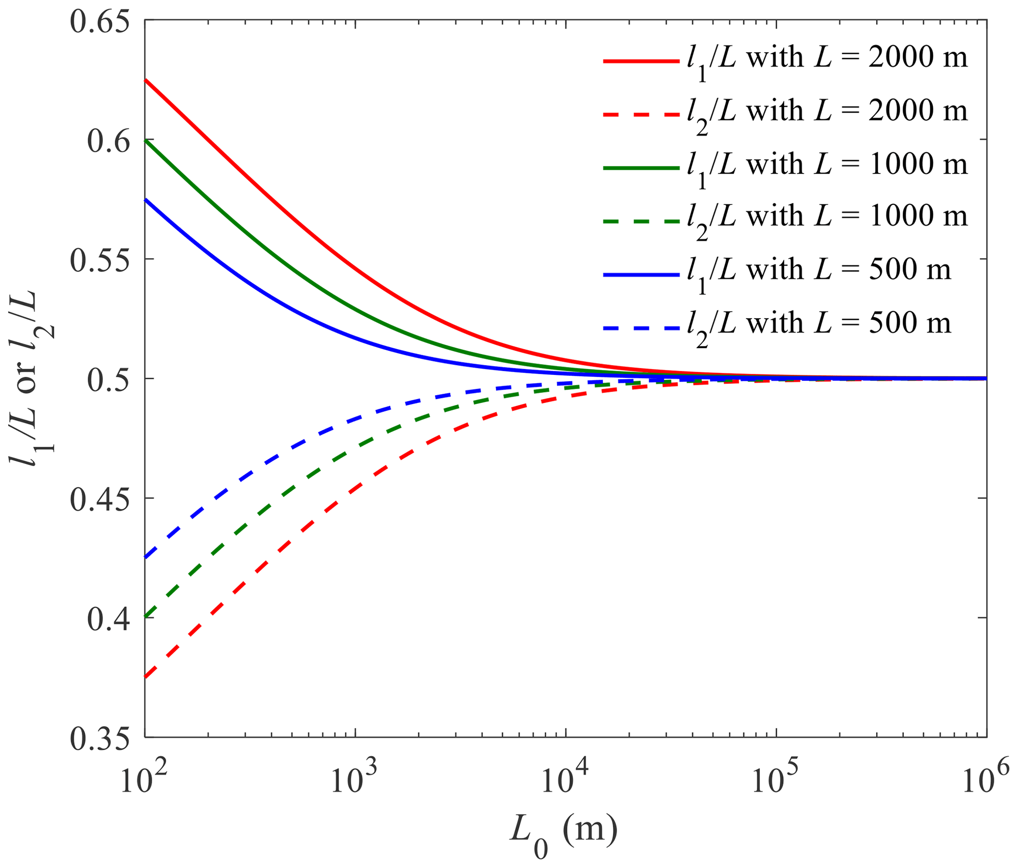
Previous studies showed that boundary conditions play a critical role in estimates of seawater intrusion (Werner and Simmons, 2009; Lu et al., 2016). Therefore, the internal no-flow boundary between the sea and lagoon was examined for various ASAs. As indicated by Eqs. (15) and (16), this internal no-flow boundary depends only on L and L0. The values of l1 and l2 calculated respectively from Eqs. (15) and (16) are shown in Fig. 4 for three typical values of L (500, 1000 and 2000 m), with L0 varying from 102 to 106 m. In general, the internal no-flow boundary deviates from the middle of the ASA. When L0 is less than 105 m, l1 is larger than l2 for the three different values of L, indicating an internal no-flow boundary closer to the lagoon boundary. For example, taking L=2000 m and L0=100 m leads to l1=1240 m and l2=760 m, with a deviation of 240 m (12 % of 2000 m) from the middle of the ASA. When L0 exceeds 105 m, however, the location of the internal no-flow boundary can be approximated as being at the middle of the ASA for all considered values of L. This is in contrast to strip and circular aquifers, where the internal no-flow boundary is always in the middle of the aquifer due to symmetry.
Since the internal no-flow boundary location between the sea and lagoon deviates from the middle of the ASA, we expect aquifer geometry to play a significant role in controlling seawater intrusion. As mentioned previously, ASAs can be convergent (Unit 1) or divergent aquifers (Unit 2) where the extent of seawater intrusion may be different. However, for strip aquifers, both Units 1 and 2 are rectangular with the same extent of seawater intrusion. Therefore, three geometries were compared in this study: convergent, rectangular and divergent (Fig. 5). These geometries have been widely examined in hillslope hydrology regrading to the effects of aquifer geometry on runoff generation (Troch et al., 2003; Kong et al., 2016; Luo et al., 2018). To present the results more conveniently, we placed the r−z coordinate origin at the intersection of the constant-head boundary (sea or lagoon) and the impermeable base, with the r axis pointing horizontally to the internal no-flow boundary and the z axis vertically upward (Fig. 5). In addition, the distance between the constant-head boundary and the internal no-flow boundary (aquifer width) is denoted as L* (Fig. 5), while the other parameters remain the same.
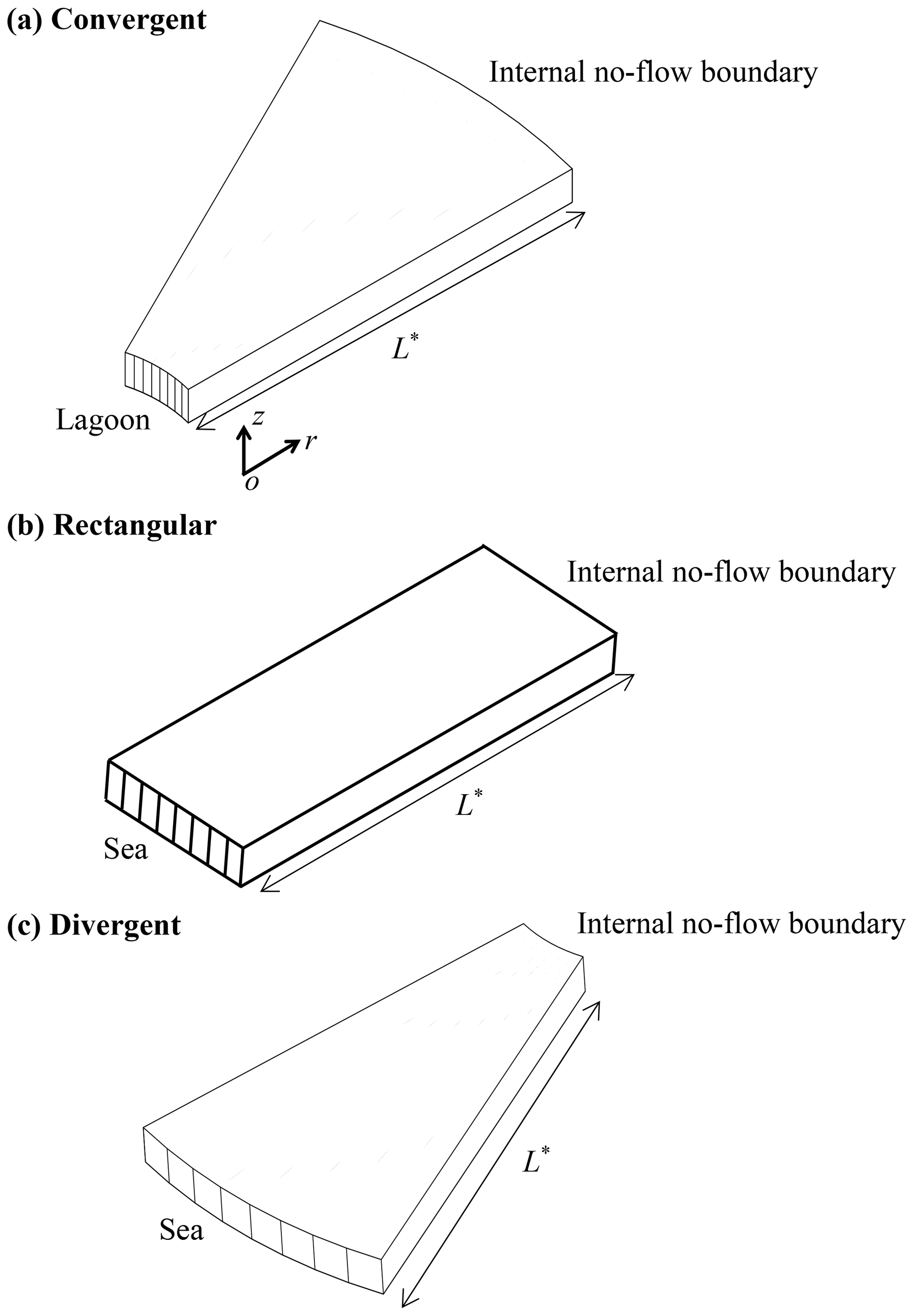
Figure 5Three-dimensional view of (a) convergent (smaller side facing the lagoon), (b) rectangular and (c) divergent aquifers (larger side facing the sea) compared in this study. L* represents the distance from the sea/lagoon to the internal no-flow boundary, i.e., l1 or l2 in Fig. 2. The internal no-flow boundary corresponds to the z axis in Fig. 2.
Following previous studies (e.g., Lu et al., 2016, 2019), different cases were selected to show the effects of aquifer geometry on seawater intrusion (Cases 1 and 2 in Table 1). According to Werner et al. (2017), the width of atoll islands generally varies from 100 to 1500 m along the radial direction. In order to focus on the effects of aquifer geometry on seawater intrusion, the same L* and L0 were assumed for the three aquifers, with L* and L0 equal to 1000 and 200 m, respectively. Note that L0 is the distance from the circle center to the lagoon boundary for convergent aquifers, whereas it represents the distance from the circle center to internal no-flow boundary for divergent aquifers hereafter. The sand characteristics were the same as in the experiments of Memari et al. (2020). Two recharge events were considered (Cases 1 and 2, Table 1). The freshwater–seawater interface was calculated using the analytical solutions for the three different aquifers. Note that the Appendix presents analytical solutions for seawater intrusion in strip aquifers deduced from Lu et al. (2019).
Table 1List of parameters use in different simulations.

* The parameter is varied: the range of L0 is from 200 to 6000 m, whereas the range of L* is from 600 to 1600 m.
Figure 6 shows the freshwater–seawater interface calculated for Cases 1 and 2. As can be seen, the extent of seawater intrusion is noticeably different for the three aquifer geometries. For high recharge ( m s−1), the interface tip is located at around 500 m for the divergent aquifer, which is about twice the value of the rectangular aquifer and 6 times the value for the convergent aquifer (Fig. 6a). When the recharge decreases to m s−1, the interface tip moves further landward for the three aquifers as expected, but the difference between results is still great (Fig. 6b). The interface tip is displaced above the aquifer bed for both the rectangular and divergent aquifers, while it remains on the aquifer bed for the convergent aquifer. Regardless of the recharge rate, the most landward freshwater–seawater interface occurs in the divergent aquifer and vice versa for the convergent aquifer. This underlines that aquifer geometry plays a major role in controlling seawater intrusion, and hence it is necessary to account for aquifer geometry in analyses of seawater intrusion.
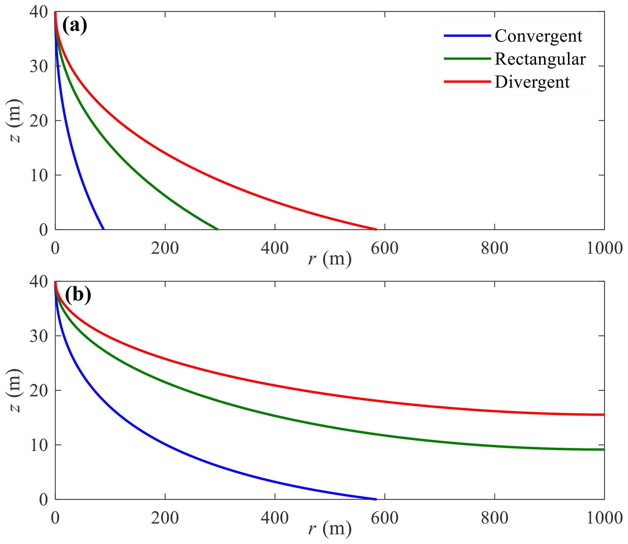
Figure 6Freshwater–seawater interface predicted by analytical solutions for three different aquifers with (a) high and (b) low recharge (Cases 1 and 2 in Table 1). Note that r=1000 m is the internal no-flow boundary in Fig. 5.

Figure 7Sensitivity of (a, b) the locations of the freshwater–seawater interface and (c, d) watertable to L0 for convergent (a, c) and divergent (b, d) aquifers. The arrow in each plot shows the direction of increasing L0 (values given in a, used to produce the different curves). Note that predictions for rectangular aquifers are independent of L0.
4.3 Sensitivity analysis
A sensitivity analysis was conducted to investigate to what extent aquifer geometry affects seawater intrusion. Since we focus on the effects of aquifer geometry on the locations of the freshwater–seawater interface and watertable, values of L0 and L* were varied, with other parameters kept constant. When conducting the sensitivity analysis of L0, L* was fixed at 1000 m, which is a typical value for ASAs (Werner et al., 2017). Figure 7 shows the sensitivity of the locations of the freshwater–seawater interface and watertable to changes in L0 (Case 3, Table 1). The freshwater–seawater interface and watertable elevation are independent of L0 for rectangular aquifers (Appendix A). However, the freshwater–seawater interface and watertable elevation differ greatly when varying L0 for both convergent and divergent aquifers, highlighting that L0 plays an important role in affecting seawater intrusion. Specifically, as L0 increases, the freshwater–seawater interface moves more landward (larger , Fig. 7a), and its corresponding watertable elevation decreases (Fig. 7c) for convergent aquifers. In contrast, for divergent aquifers, increasing L0 moves the freshwater–seawater interface more seaward (smaller , Fig. 7b), and its corresponding watertable elevation increases (Fig. 7d). For a given L0, divergent aquifers have the largest extent of seawater intrusion and the lowest watertable elevation, and the opposite is the case for convergent aquifers (Fig. 7).
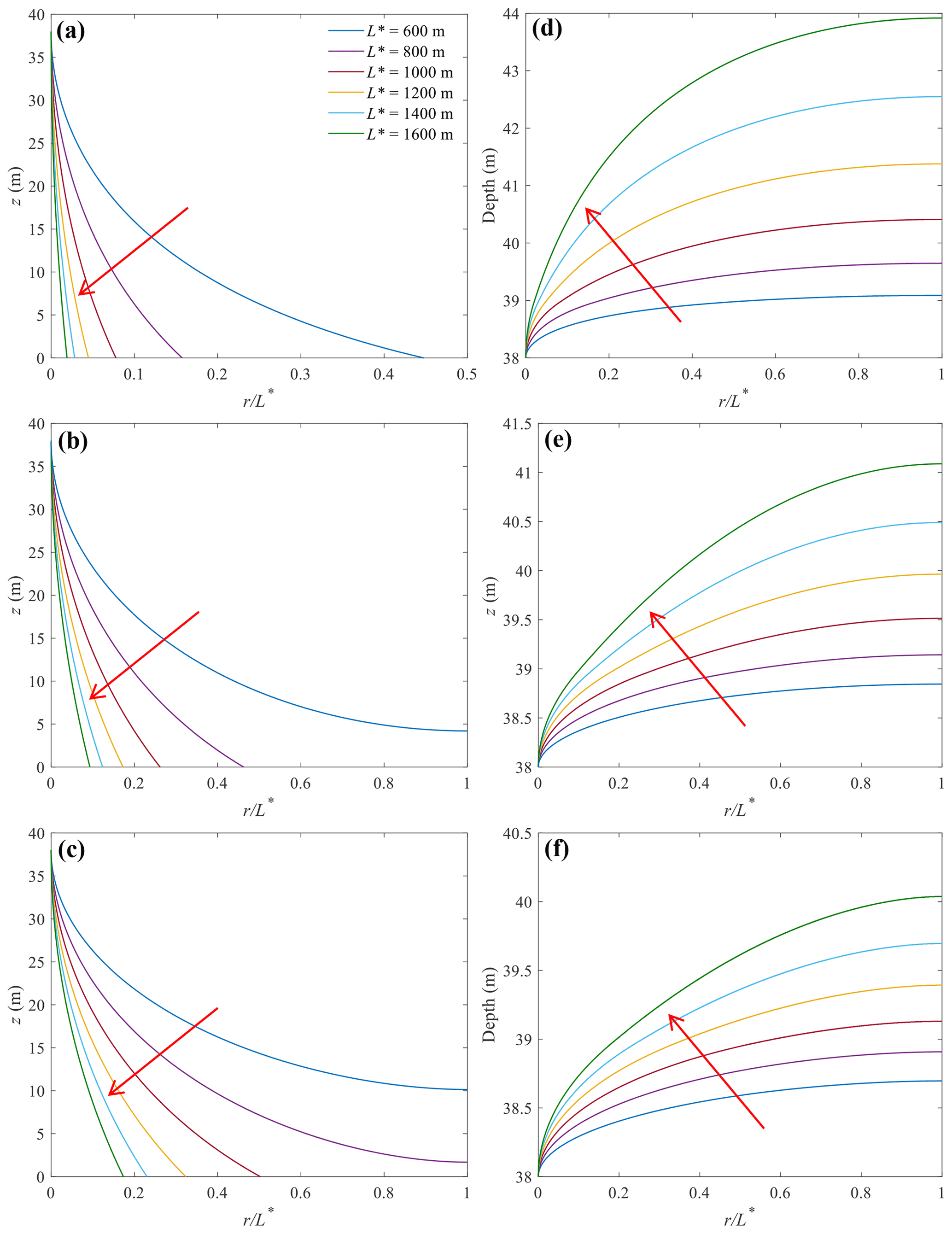
Figure 8Sensitivity of (a–c) the locations of the freshwater–seawater interface and (d–f) watertable to L* for convergent (a, d), rectangular (b, e) and divergent (c, f) aquifers. The arrow in each plot points to the increase in L* values used to construct each curve (values indicated in a).
Regardless of the freshwater–seawater interface and watertable elevation, the deviation between rectangular aquifers and divergent or convergent aquifers is significant when L0 is less than 2000 m (Fig. 7). For example, the r coordinate of the interface tip (z=0) is 262 m for the rectangular aquifer at L0=200 m, whereas it is 78 (31 % of that in the rectangular aquifer) and 500 m (191 % of that in the rectangular aquifer) for the convergent and divergent aquifers, respectively. As L0 increases, the deviation between the three aquifers decreases. When L0=2000 m, the r coordinate of the interface tip is 262, 209 (80 % of that in the rectangular aquifer) and 318 m (121 % of that in the rectangular aquifer) for the rectangular, convergent and divergent aquifers, respectively. As L0 increases to 6000 m, the freshwater–seawater interface and watertable elevation of both convergent and divergent aquifers tend to those of rectangular aquifers; i.e., geometry effects decrease with increasing L0. These results highlight the critical role played by the shape of aquifers. As a result, ignoring the aquifer geometry may lead to an inappropriate management strategy for groundwater resources in atoll islands.
The sensitivity of the freshwater–seawater interface and watertable elevation to L* was investigated by varying L* from 600 to 1600 m while fixing L0 to 200 m (Case 4, Table 1). As shown in Fig. 8, contrary to the results for varying L0, in this case the freshwater–seawater interface and watertable elevation in all three topographies are related to L*. Again, the extent of seawater intrusion is greatest in divergent aquifers and least in convergent aquifers for a given L*. When L* increases, the freshwater–seawater interface moves seaward, and the watertable elevation increases, regardless of aquifer geometry; i.e., the seawater intrusion decreases (Fig. 8a–c). This is because the total freshwater flux increases with increasing L*, leading to a higher hydraulic gradient and hence less seawater intrusion (Fig. 8d–f). Moreover, an increase in L* reduces the differences in the seawater intrusion distance among the three geometries; i.e., the effects of aquifer geometry on seawater intrusion are more significant at small L*. However, even at the maximum L* considered (1600 m), the deviation between three aquifers remains significant: the r coordinate of the interface tip is about 148 m for the rectangular aquifer, whereas it is about 32 (22 % of that in the rectangular aquifer) and 278 m (188 % of that in the rectangular aquifer) for the convergent and divergent aquifers, respectively. Both L0 and L* can greatly impact seawater intrusion estimates for divergent and convergent aquifers, highlighting the necessity to include geometry effects in analytical solutions of seawater intrusion.
Based on the Ghijben–Herzberg and hillslope-storage Boussinesq equations, we derived analytical solutions of steady-state seawater intrusion for ASAs, with a focus on the freshwater–seawater interface and its corresponding watertable elevation as affected by recharge. After comparing with experimental data of Memari et al. (2020), the analytical solutions were employed to examine the effects of aquifer geometry on seawater intrusion in island aquifers. Three different shapes of island aquifer were compared: convergent, rectangular and divergent. The results lead to the following conclusions.
-
The presented analytical solutions perform well in predicting the experimental freshwater–seawater interface, suggesting that these analytical solutions can predict seawater intrusion reasonably in different aquifer geometries.
-
Island geometry plays a significant role in affecting the freshwater–seawater interface and watertable elevation. Other factors being equal, the extent of seawater intrusion is greatest in divergent aquifers and conversely least in convergent aquifers. In contrast, the watertable elevation is lowest in divergent aquifers and highest in convergent aquifers.
-
The effects of aquifer geometry on seawater intrusion are dependent on the aquifer width and distance from the circle center to the internal no-flow boundary (Figs. 7 and 8). A larger aquifer width and distance from the circle center to the inner arc (the lagoon boundary for convergent aquifers or the internal no-flow boundary for divergent aquifers) weaken the role played by aquifer geometry and hence lead to a smaller deviation of the extent of seawater intrusion between the three topographies.
Real island aquifers are expected to exhibit more complexity than considered here; e.g., they will have more complex shapes and are subjected to transient flow conditions caused by tides, waves and groundwater pumping (Mantoglou, 2003; Pool and Carrera, 2011; Werner et al., 2013). In addition, since the experimental scale of Memari et al. (2020) is necessarily small, future experiments and field data are needed to further validate and facilitate the analytical solutions. Despite this, the new analytical solutions, validated against experiments, can be used as a tool for rapid estimation of seawater intrusion in ASAs once known island geometry and corresponding soil properties are given.
For rectangular aquifers, the seawater intrusion in Unit 1 is identical to that in Unit 2 because of symmetry. With the interface tip on the aquifer bed, analytical solutions for the freshwater–seawater interface (hs), watertable elevation (h), and r coordinate of the interface tip in Unit 2 (rt2) can be respectively written as (Lu et al., 2019)
When the interface tip is above the aquifer bed, the analytical solution for the freshwater–seawater interface location and watertable elevation in Unit 2 are the same as Eqs. (A1) and (A2), respectively.
Experimental data used in this study were compiled from Memari et al. (2020).
All the authors contributed to the design of the research. ZL carried out data collation, developed the analytical solutions and prepared the manuscript with contributions from all the co-authors. All the authors contributed to the interpretation of the results and provided feedback.
The contact author has declared that neither they nor their co-authors have any competing interests.
Publisher's note: Copernicus Publications remains neutral with regard to jurisdictional claims in published maps and institutional affiliations.
This research was supported by the National Key R & D Program of China (2019YFC0409004) and the National Natural Science Foundation of China (51979095 and 41807178). Zhaoyang Luo acknowledges EPFL for financial support, and Jun Kong acknowledges the Qing Lan Project of Jiangsu Province (2020). We appreciate the constructive comments from the handling editor Mauro Giudici and three anonymous reviewers, which led to significant improvement to the paper.
This research has been supported by the National Key R & D Program of China (2019YFC0409004), the National Natural Science Foundation of China (51979095 and 41807178), EPFL and the Qing Lan Project of Jiangsu Province (2020).
This paper was edited by Mauro Giudici and reviewed by three anonymous referees.
Ayers, J. F. and Vacher, H. L.: Hydrogeology of an atoll island: A conceptual model from detailed study of a Micronesian example, Groundwater, 24, 185–198, https://doi.org/10.1111/j.1745-6584.1986.tb00994.x, 1986.
Bailey, R. T., Jenson, J. W., and Olsen, A. E.: Numerical modeling of atoll island hydrogeology, Groundwater, 47, 184–196, https://doi.org/10.1111/j.1745-6584.2008.00520.x, 2009.
Bailey, R. T., Jenson, J. W., and Olsen, A. E.: Estimating the ground water resources of atoll islands, Water, 2, 1–27, https://doi.org/10.3390/w2010001, 2010.
Bedekar, V. S., Memari, S. S., and Clement, T. P.: Investigation of transient freshwater storage in island aquifers, J. Contam. Hydrol., 221, 98–107, https://doi.org/10.1016/j.jconhyd.2019.02.004, 2019.
Chesnaux, R. and Allen, D. M.: Groundwater travel times for unconfined island aquifers bounded by freshwater or seawater, Hydrogeol. J., 16, 437–445, https://doi.org/10.1007/s10040-007-0241-6, 2008.
Dose, E. J., Stoeckl, L., Houben, G. J., Vacher, H. L., Vassolo, S., Dietrich, J., and Himmelsbach, T.: Experiments and modeling of freshwater lenses in layered aquifers: Steady state interface geometry, J. Hydrol., 509, 621–630, https://doi.org/10.1016/j.jhydrol.2013.10.010, 2014.
Drabbe, J. and Badon Ghijben, W.: Nota in verband met de voorgenomen put boring nabij Amsterdam, Tijdschrift van het Koninklijk Instituut van Ingenieurs, Gravenhage, the Netherlands, 8–22, 1889.
Duvat, V. K. E.: A global assessment of atoll island planform changes over the past decades, Wiley Interdisciplin. Rev. Clim. Change, 10, e557, https://doi.org/10.1002/wcc.557, 2019.
Fan, Y. and Bras, R. L.: Analytical solutions to hillslope subsurface storm flow and saturation overland flow, Water Resour. Res., 34, 921–927, https://doi.org/10.1029/97WR03516, 1998.
Fetter, C. W.: Position of the saline water interface beneath oceanic islands, Water Resour. Res., 8, 1307–1315, https://doi.org/10.1029/WR008i005p01307, 1972.
Gingerich, S. B., Voss, C. I., and Johnson, A. G.: Seawater-flooding events and impact on freshwater lenses of low-lying islands: Controlling factors, basic management and mitigation, J. Hydrol., 551, 676–688, https://doi.org/10.1016/j.jhydrol.2017.03.001, 2017.
Greskowiak, J., Röper, T., and Post, V. E.: Closed-form approximations for two-dimensional groundwater age patterns in a fresh water lens, Groundwater, 51, 629–634, https://doi.org/10.1111/j.1745-6584.2012.00996.x, 2013.
Hazenberg, P., Fang, Y., Broxton, P., Gochis, D., Niu, G. Y., Pelletier, J. D., Troch., P. A., and Zeng, X.: A hybrid-3D hillslope hydrological model for use in Earth system models, Water Resour. Res., 51, 8218–8239, https://doi.org/10.1002/2014WR016842, 2015.
Hazenberg, P., Broxton, P., Gochis, D., Niu, G. Y., Pangle, L. A., Pelletier, J. D., Troch., P. A., and Zeng, X.: Testing the hybrid-3-D hillslope hydrological model in a controlled environment, Water Resour. Res., 52, 1089–1107, https://doi.org/10.1002/2015WR018106, 2016.
Herzberg, A.: Die wasserversorgung einiger Nordseebäder, J. Gasbeleucht. Wasserversorg., 44, 815–819, 45, 842–844, 1901.
Hilberts, A. G., Troch, P. A., Paniconi, C., and Boll, J.: Low-dimensional modeling of hillslope subsurface flow: Relationship between rainfall, recharge, and unsaturated storage dynamics, Water Resour. Res., 43, W03445, https://doi.org/10.1029/2006WR004964, 2007.
Hilberts, A. G. J., Troch, P. A., and Paniconi, C.: Storage-dependent drainable porosity for complex hillslopes, Water Resour. Res., 41, W06001, https://doi.org/10.1029/2004WR003725, 2005.
Ketabchi, H., Mahmoodzadeh, D., Ataie-Ashtiani, B., Werner, A. D., and Simmons, C. T.: Sea-level rise impact on fresh groundwater lenses in two-layer small islands, Hydrol. Process., 28, 5938–5953, https://doi.org/10.1002/hyp.10059, 2014.
Kong, J., Shen, C., Luo, Z., Hua, G., and Zhao, H.: Improvement of the hillslope-storage Boussinesq model by considering lateral flow in the unsaturated zone, Water Resour. Res., 52, 2965–2984, https://doi.org/10.1002/2015WR018054, 2016.
Lam, R. K.: Atoll permeability calculated from tidal diffusion, J. Geophys. Res., 79, 3073–3081, https://doi.org/10.1029/JC079i021p03073, 1974.
Liu, J. and Tokunaga, T.: Future risks of tsunami-induced seawater intrusion into unconfined coastal aquifers: Insights from numerical simulations at Niijima Island, Japan, Water Resour. Res., 55, 10082–10104, https://doi.org/10.1029/2019WR025386, 2019.
Liu, Y., Mao, X., Chen, J., and Barry, D. A.: Influence of a coarse interlayer on seawater intrusion and contaminant migration in coastal aquifers, Hydrol. Process., 28, 5162–5175, https://doi.org/10.1002/hyp.10002, 2014.
Lu, C., Xin, P., Kong, J., Li, L., and Luo, J.: Analytical solutions of seawater intrusion in sloping confined and unconfined coastal aquifers, Water Resour. Res., 52, 6989–7004, https://doi.org/10.1002/2016WR019101, 2016.
Lu, C., Cao, H., Ma, J., Shi, W., Rathore, S. S., Wu, J., and Luo, J.: A proof-of-concept study of using a less permeable slice along the shoreline to increase fresh groundwater storage of oceanic islands: Analytical and experimental validation, Water Resour. Res., 55, 6450–6463, https://doi.org/10.1029/2018WR024529, 2019.
Luo, Z., Shen, C., Kong, J., Hua, G., Gao, X., Zhao, Z., Zhao, H., and Li, L.: Effects of unsaturated flow on hillslope recession characteristics, Water Resour. Res., 54, 2037–2056, https://doi.org/10.1002/2017WR022257, 2018.
Mantoglou, A.: Pumping management of coastal aquifers using analytical models of saltwater intrusion, Water Resour. Res., 39, 1335, https://doi.org/10.1029/2002WR001891, 2003.
Memari, S. S., Bedekar, V. S., and Clement, T. P.: Laboratory and numerical investigation of saltwater intrusion processes in a circular island aquifer, Water Resour. Res., 56, e2019WR025325, https://doi.org/10.1029/2019WR025325, 2020.
Morgan, L. K. and Werner, A. D.: Seawater intrusion vulnerability indicators for freshwater lenses in strip islands, J. Hydrol., 508, 322–327, https://doi.org/10.1016/j.jhydrol.2013.11.002, 2014.
Paniconi, C., Troch, P. A., Van Loon, E. E., and Hilberts, A. G.: Hillslope-storage Boussinesq model for subsurface flow and variable source areas along complex hillslopes: 2. Intercomparison with a three-dimensional Richards equation model, Water Resour. Res., 39, 1317, https://doi.org/10.1029/2002WR001730, 2003.
Pool, M. and Carrera, J.: A correction factor to account for mixing in Ghyben-Herzberg and critical pumping rate approximations of seawater intrusion in coastal aquifers, Water Resour. Res., 47, W05506, https://doi.org/10.1029/2010WR010256, 2011.
Post, V. E.: Annotated translation of “Nota in verband met de voorgenomen putboring nabij Amsterdam [Note concerning the intended well drilling near Amsterdam]” by J. Drabbe and W. Badon Ghijben (1889), Hydrogeol. J., 26, 1771–1788, https://doi.org/10.1007/s10040-018-1797-z, 2018.
Post, V. E. A., Houben, G. J., Stoeckl, L., and Sültenfuß, J.: Behaviour of tritium and tritiogenic helium in freshwater lens groundwater systems: Insights from Langeoog Island, Germany, Geofluids, 2019, 1494326, https://doi.org/10.1155/2019/1494326, 2019.
Röper, T., Greskowiak, J., Freund, H., and Massmann, G.: Freshwater lens formation below juvenile dunes on a barrier island (Spiekeroog, Northwest Germany), Estuar. Coast. Shelf Sci., 121–122, 40–50, https://doi.org/10.1016/j.ecss.2013.02.004, 2013.
Stoeckl, L., Houben, G. J., and Dose, E. J.: Experiments and modeling of flow processes in freshwater lenses in layered island aquifers: Analysis of age stratification, travel times and interface propagation, J. Hydrol., 529, 159–168, https://doi.org/10.1016/j.jhydrol.2015.07.019, 2015.
Storlazzi, C. D., Gingerich, S. B., van Dongeren, A., Cheriton, O. M., Swarzenski, P. W., Quataert, E., Voss, C. I., Field, D. W., Annamalai, H., Piniak, G. A., and McCall, R.: Most atolls will be uninhabitable by the mid-21st century because of sea-level rise exacerbating wave-driven flooding, Sci. Adv., 4, eaap9741, https://doi.org/10.1126/sciadv.aap9741, 2018.
Stuyfzand, P. J.: Hydrochemistry and hydrology of the coastal dune area of the Western Netherlands, PhD Thesis, Vrije University, Amsterdam, ISBN 90-74741-01-0, available at: http://dare.ubvu.vu.nl/handle/1871/12716 (last access: 21 December 2021), 1993.
Stuyfzand, P. J.: Observations and analytical modeling of freshwater and rainwater lenses in coastal dune systems, J. Coast. Conserv., 21, 577–593, https://doi.org/10.1007/s11852-016-0456-6, 2017.
Thomas, A., Baptiste, A., Martyr-Koller, R., Pringle, P., and Rhiney, K.: Climate change and small island developing states, Annu. Rev. Environ. Resour., 45, 1–27, https://doi.org/10.1146/annurev-environ-012320-083355, 2020.
Troch, P. A., Paniconi, C., and van Loon, E.: Hillslope-storage Boussinesq model for subsurface flow and variable source areas along complex hillslopes: 1. Formulation and characteristic response, Water Resour. Res., 39, 1316, https://doi.org/10.1029/2002WR001728, 2003.
Underwood, M. R., Peterson, F. L., and Voss, C. I.: Groundwater lens dynamics of atoll islands, Water Resour. Res., 28, 2889–2902, https://doi.org/10.1029/92WR01723, 1992.
Vacher, H. L.: Dupuit-Ghyben-Herzberg analysis of strip-island lenses, Geol. Soc. Am. Bull., 100, 580–591, https://doi.org/10.1130/0016-7606(1988)100<0580:DGHAOS>2.3.CO;2, 1988.
Werner, A. D. and Simmons, C. T.: Impact of sea-level rise on sea water intrusion in coastal aquifers, Groundwater, 47, 197–204, https://doi.org/10.1111/j.1745-6584.2008.00535.x, 2009.
Werner, A. D., Bakker, M., Post, V. E., Vandenbohede, A., Lu, C., Ataie-Ashtiani, B., Simmons, C. T., and Barry, D. A.: Seawater intrusion processes, investigation and management: Recent advances and future challenges, Adv. Water Resour., 51, 3–26, https://doi.org/10.1016/j.advwatres.2012.03.004, 2013.
Werner, A. D., Sharp, H. K., Galvis, S. C., Post, V. E., and Sinclair, P.: Hydrogeology and management of freshwater lenses on atoll islands: Review of current knowledge and research needs, J. Hydrol., 551, 819–844, https://doi.org/10.1016/j.jhydrol.2017.02.047, 2017.
White, I. and Falkland, T.: Management of freshwater lenses on small Pacific islands, Hydrogeol. J., 18, 227–246, https://doi.org/10.1007/s10040-009-0525-0, 2010.
Zhang, Y., Li, L., Erler, D. V., Santos, I., and Lockington, D.: Effects of alongshore morphology on groundwater flow and solute transport in a nearshore aquifer, Water Resour. Res., 52, 990–1008, https://doi.org/10.1002/2015WR017420, 2016.