Flexible and consistent quantile estimation for intensity–duration–frequency curves

Assessing the relationship between the intensity, duration, and frequency (IDF) of extreme precipitation is required for the design of water management systems. However, when modeling sub-daily precipitation extremes, there are commonly only short observation time series available. This problem can be overcome by applying the duration-dependent formulation of the generalized extreme value (GEV) distribution which fits an IDF model with a range of durations simultaneously. The originally proposed duration-dependent GEV model exhibits a power-law-like behavior of the quantiles and takes care of a deviation from this scaling relation (curvature) for sub-hourly durations (Koutsoyiannis et al., 1998). We suggest that a more flexible model might be required to model a wide range of durations (1 min to 5 d). Therefore, we extend the model with the following two features: (i) different slopes for different quantiles (multiscaling) and (ii) the deviation from the power law for large durations (flattening), which is newly introduced in this study. Based on the quantile skill score, we investigate the performance of the resulting flexible model with respect to the benefit of the individual features (curvature, multiscaling, and flattening) with simulated and empirical data. We provide detailed information on the duration and probability ranges for which specific features or a systematic combination of features leads to improvements for stations in a case study area in the Wupper catchment (Germany). Our results show that allowing curvature or multiscaling improves the model only for very short or long durations, respectively, but leads to disadvantages in modeling the other duration ranges. In contrast, allowing flattening on average leads to an improvement for medium durations between 1 h and 1 d, without affecting other duration regimes. Overall, the new parametric form offers a flexible and enhanced performance model for consistently describing IDF relations over a wide range of durations, which has not been done before as most existing studies focus on durations longer than 1 h or day and do not address the deviation from the power law for very long durations (2–5 d).

1 Introduction

The number of heavy precipitation events has increased significantly in Europe (Kundzewicz et al., 2006; Tank and Können, 2003) and worldwide (Hartmann et al., 2013). Such events are related to flooding and other hazards which can cause severe damage to agriculture and infrastructure (Brémond et al., 2013). The impact of extreme precipitation depends on the temporal scale of the event. Short, intense convective precipitation exhibits different characteristic consequences than long-lasting, mostly stratiform, precipitation. Examples for events on different timescales of minutes to hours, days, and weeks are pluvial or flash floods (Braunsbach, Germany, May 2016), river flooding (Elbe, Germany, 2013), and groundwater flooding (Leicestershire, UK, March 2017), respectively.

The definition of precipitation extremes is based on the occurrence probability and is quantified using quantiles (return levels) and associated occurrence probabilities, often expressed as return periods in a stationary interpretation. Quantitative estimations of quantiles and associated probabilities mostly follow one of two popular methods, namely (1) block maxima and their description with the generalized extreme value (GEV) distribution – a heavy-tailed and asymmetric distribution – or (2) threshold exceedances and a description with the generalized Pareto distribution (GPD; e.g., Coles, 2001). Typically, annual precipitation maxima of different timescales are used to describe extreme rainfall events. Both GEV and GPD can be used to model the extreme precipitation of a certain timescale. A common problem for short timescales, i.e., the scarce availability of data with high measurement frequency, can be overcome by modeling several timescales at once. Different timescales can be represented as durations over which the precipitation rate is aggregated and averaged. Most frequently, daily precipitation sums are reported but hourly or 5 min aggregation are also common.

A way to describe the characteristics of extremes for various durations (timescales) are intensity–duration–frequency (IDF) curves, which describe the relationship between extreme precipitation intensities, their duration (timescale), and their frequency (occurrence probability or average return period). These relations have been known since the mid-20th century (Chow, 1953) and have become popular among hydrologists and meteorologists. In estimating these curves, one tries to exploit the assumption of a smooth intensity–frequency relationship across different durations. This helps for interpolating between durations, and it can also improve the estimation for short durations, as shorter time series are often available for those.

Historically, a set of GEV distributions is sought individually for a set of durations (e.g., 5 min, 1 h, 12 h, 24 h, and 48 h) leading to quantile (return level) estimates for specified probabilities (return periods) for all durations considered. In a second step, for a given probability a smooth function is estimated by interpolating associated quantiles across durations (García-Bartual and Schneider, 2001). However, by using a duration-dependent extreme value distribution (d-GEV) (see the first examples in Nguyen et al., 1998, and Menabde et al., 1999), IDF estimation can be carried out in one step within a single model. To achieve this, GEV parameters are defined as functions of duration. This approach prevents the crossing of quantiles across durations and is, thus, considered consistent. Moreover, the data are used more efficiently, which simplifies the extension of the model, e.g., the inclusion of large-scale covariates at a later stage. This will enable first insights into physical effects beyond the pure statistical evaluation of precipitation.

It is widely agreed that precipitation intensities for given exceedance probabilities follow a power-law-like function (scaling) across duration (Gupta and Waymire, 1990; Veneziano and Furcolo, 2002; Burlando and Rosso, 1996), with higher intensities for short durations. For a range of very short durations (d≤1 h), the scaling assumption does not hold because maxima from different durations often originate from the same event. This leads to a curvature of IDF curves, where intensity no longer follows a power law with decreasing duration. Bougadis and Adamowski (2006) approached this issue by using two different duration exponents for small durations and for other durations. A more smooth transition can be achieved by including the curvature as a duration offset in the parameters of the GEV distribution without explicitly distinguishing between short and long durations. Koutsoyiannis et al. (1998) used a model with five parameters to describe the complete IDF relation for different probabilities (return periods) and across durations. The underlying idea is based on a reparameterization of the GEV and its three characteristic parameters of location μ, scale σ, and shape ξ. While shape ξ is held constant for all durations d, it is further assumed that the ratio between location and scale $\mathit{\mu }/\mathit{\sigma }$ remains constant across duration d (for details, see Sect. 2.3).

Ulrich et al. (2020) built on the approach of Koutsoyiannis et al. (1998) and extended it to a spatial setting with covariates for the d-GEV parameters. Although using both consistent modeling and spatial pooling improves model performance, the need for more flexibility of the IDF curves in longer durations is emphasized and will be addressed in the present study. Therefore, we aim to look for new parameterizations of the IDF curve's duration dependence by combining the existing approaches of multiscaling and duration offset and also extending it by a new parameter, namely the intensity offset.

The commonly used variant of the d-GEV with five parameters (Koutsoyiannis et al., 1998) might not be flexible enough for a wide range of durations from minutes to several days. A first approach for extending the d-GEV addresses the simple scaling relation. This model assumes a scaling that is independent of the exceedance probability (return period). However, relaxing this assumption leads to so-called multiscaling, which allows for different scaling-like behavior for different exceedance probabilities (return periods). This is achieved by introducing another parameter η₂, as in Eqs. 8 and 10 in Sect. 2.3. Then, the ratio between location and scale is not constant anymore. Multiscaling is found to be effective for durations longer than 1 h (Veneziano and Furcolo, 2002; Burlando and Rosso, 1996). Van de Vyver (2018) employs the multiscaling approach in a Bayesian setting. On a global scale, different scale parameters have been investigated by Courty et al. (2019). None of the named studies combine multiscaling with curvature for short durations but focus on only one of these aspects, while our study is aiming for a combination and analysis of three different features.

In this study, we compare different ways to parameterize IDF curves, including the features of multiscaling and duration offset. In addition, we present a new d-GEV parameter, the intensity offset, which accounts for the deviation from the power law and the flattening of IDF curves for long durations. To our knowledge, this comprehensive analysis of different features has not been conducted before. Section 2 lists the data sources and introduces the different features and their modeling equations, as well as the verification methods, to analyze modeling performance. In Sect. 3, the cross-validated verification results of all features are shown with respect to modeling performance of different return periods and durations. For verification, we perform a case study using rainfall gauge data from a catchment in Germany. IDF curves that include all analyzed features are presented for selected stations.

2 Data and methods

We use precipitation measurements in an area in and around the catchment of the river Wupper in western Germany. In order to compare different models for the d-GEV, we use the quantile skill index (QSI) introduced in Ulrich et al. (2020) within a cross-validation setting. For the resulting IDF curves, we obtain confidence intervals using a bootstrapping method and test their coverage with artificial data with known dependence levels in a simulation study. The data and all necessary methods are explained in the following section.

2.1 Station-based precipitation data

Precipitation sums for the minute, hour, and day are provided by Wupperverband and the German Meteorological Service. Rain gauges are located in and around the catchment of the river Wupper in North Rhine–Westphalia, Germany. In total, 115 stations are used. Data from two measuring devices with a distance below 250 m are combined into one station each in order to obtain a longer time series, thus resulting in a total of 92 grouped stations. However, in cases where measurement series are grouped together, it is common to have measurements from both instruments for a certain period of time. Thus, when merging, we decided to use only the observations with the higher measuring frequency for the analysis. For example, when combining two time series with hourly and daily data, respectively, the time series of all aggregation levels (durations) are obtained from the hourly data for the overlapping period. This choice is made because 24 h values from an hourly measurement frequency might show higher intensities since the 24 h window is shifted hour by hour in order to find the annual maximum. On the other hand, 24 h values from the daily measurement frequency are recorded for a fixed day block, i.e., from 08:00 to 07:59 LT (local time). A test of robustness was performed (not shown) to assess how the estimated IDF curves are affected by the choice of measurement frequency which is preserved during the time of overlap when merging the time series. For this purpose, two IDF curves were created, i.e., (1) choosing the maxima from a higher measurement frequency and (2) choosing the maxima from a lower measurement frequency. In most cases, there was no relevant difference between both methods.

Years with more than 10 % of missing values are disregarded. Some years contain measurement artifacts, where identical rainfall values were repeated over several time steps. After consulting the data maintainers, these years are removed before the analysis. The data exhibit heterogeneity in terms of the temporal frequency and the length of the resulting time series. Figure 1 presents the availability of data over time (left) and space (right) for three possible temporal resolutions. More specifically, minute data have been available since 1968, whereas daily records range back to 1893.

Figure 1 (a) Number of stations according to the temporal resolution. (b) Station location (circles) with data availability (circle area size) by temporal resolution (color). The red line within the map of Germany indicates the Wupper catchment boundary.

Time series for different durations are obtained from an accumulation over a sample of durations as follows:

$$\begin{array}{}\text{(1)}& \begin{array}{rl}d\in \mathit{\{}& \mathrm{1}\min ,\mathrm{4}\min ,\mathrm{8}\min ,\mathrm{16}\min ,\mathrm{32}\min ,\mathrm{1}\mathrm{h},\mathrm{2}\mathrm{h},\mathrm{4}\mathrm{h},\mathrm{8}\mathrm{h},\\ & \mathrm{16}\mathrm{h},\mathrm{24}\mathrm{h},\mathrm{48}\mathrm{h},\mathrm{72}\mathrm{h},\mathrm{96}\mathrm{h},\mathrm{120}\mathrm{h}\mathit{\}},\end{array}\end{array}$$

respectively, as done by Ulrich et al. (2020). In the following, numerical values are presented in hours. We use only the annual maxima of these time series to model the distribution of extreme precipitation. The original precipitation time series are accumulated with the R package IDF (Ulrich et al., 2021b). The data set with annual maxima can be found online and supports the findings of this study (Fauer et al., 2021).

The set of durations d is chosen such that small durations are presented with smaller increments than larger durations. In a simulation study, we tested whether using a different set of durations with a stronger focus on short durations affects the results, but no such effect could be found (see Appendix C).

Minute measurements might be less accurate when only a small number of rain drops is recorded and measured intensity is affected by sampling uncertainty. However, for events that are identified as annual maxima, we expect the rain amount to be large enough so that a higher sampling uncertainty compared to larger measurement accumulation sums can be neglected.

2.2 Generalized extreme value distribution

One of the most prominent ideas of extreme value statistics is based on the Fisher–Tippett–Gnedenko theorem, which states that, under suitable assumptions, maxima drawn from sufficiently large blocks follow one of three distributions. These distributions differ in their tail behavior. The GEV distribution comprises all three cases in one parametric family and is widely used in extreme precipitation analysis as follows (Coles, 2001):

$$\begin{array}{}\text{(2)}& G\left(z\right)=\exp \mathit{\{}-{\left[\mathrm{1}+\mathit{\xi }\left({\displaystyle \frac{z-\mathit{\mu }}{\mathit{\sigma }}}\right)\right]}^{-\mathrm{1}/\mathit{\xi }}\mathit{\}}.\end{array}$$

Here, the non-exceedance probability G for precipitation intensity z depends on the parameter location μ, scale σ>0, and shape ξ≠0, with z restricted to $\mathrm{1}+\mathit{\xi }(z-\mathit{\mu })/\mathit{\sigma }>\mathrm{0}$. The non-exceedance probability can be expressed as a return period, e.g., for an annual block size $T\left(z\right)=\mathrm{1}/(\mathrm{1}-G(z\left)\right)$ years. Consequently, return values for a given non-exceedance probability $\mathrm{0}<p<\mathrm{1}$ can be calculated by solving Eq. (2) for z, as follows:

$$\begin{array}{}\text{(3)}& z=\left(\right[-\log \mathit{\left\{}p\mathit{\right\}}{]}^{-\mathit{\xi }}-\mathrm{1}){\displaystyle \frac{\mathit{\sigma }}{\mathit{\xi }}}+\mathit{\mu }.\end{array}$$

Water management authorities and other institutions rely on return values for different durations. However, the GEV distribution in the form of Eq. (2) is limited to one selected duration at a time. One way to account for that need is to model each duration separately and then, in an independent second step, interpolate the resulting quantiles (return levels) across duration d, as done in the KOSTRA atlas (DWD, 2017) of the German Meteorological Service (DWD). One huge disadvantage of this method is that quantile crossing can occur, meaning that quantiles (intensities) associated with smaller exceedance probabilities can have higher values than quantiles from larger exceedance probabilities in some duration regimes. To solve this problem, Nguyen et al. (1998), Koutsoyiannis et al. (1998), and Menabde et al. (1999) proposed a distribution with parameters depending on duration d; there is thus only one single model required to obtain consistent (i.e., non-crossing) duration dependent quantiles (return values). Another advantage is the involvement of data from neighboring durations in the estimation of GEV parameters. For the modeling of short-duration rainfall, often very little data are available than for longer durations d≥24 (1 d). Thus, in this setting, information from long durations has the potential to increase modeling performance for short durations as well.

2.3 Duration dependence

There are multiple empirical formulations for the relationship between intensity z and duration d. Koutsoyiannis et al. (1998) proposed a general form with five parameters for IDF curves. Therefore, a reparameterization and extension of the GEV is needed with the following:

$$\begin{array}{}\text{(4)}& {\displaystyle }\mathit{\sigma }\left(d\right)& {\displaystyle }={\mathit{\sigma }}_{\mathrm{0}}(d+\mathit{\theta }{)}^{-\mathit{\eta }}\text{(5)}& {\displaystyle }\mathit{\mu }\left(d\right)& {\displaystyle }=\stackrel{\mathrm{̃}}{\mathit{\mu }}\mathit{\sigma }\left(d\right)\text{(6)}& {\displaystyle }\mathit{\xi }& {\displaystyle }=\text{const.}\text{(7)}& {\displaystyle }G\left(z\right)& {\displaystyle }=\exp \mathit{\{}-{\left[\mathrm{1}+\mathit{\xi }\left({\displaystyle \frac{z}{{\mathit{\sigma }}_{\mathrm{0}}(d+\mathit{\theta }{)}^{-\mathit{\eta }}}}-\stackrel{\mathrm{̃}}{\mathit{\mu }}\right)\right]}^{-\mathrm{1}/\mathit{\xi }}\mathit{\}}.\end{array}$$

Here, $\stackrel{\mathrm{̃}}{\mathit{\mu }}$ is the rescaled location parameter, θ is the duration offset, and η the duration exponent. Scale σ follows a two-parameter power law (scaling relation) of duration d, with scale offset σ₀ being constant for all durations. For d≫θ, it is justified to disable the duration offset feature by setting duration offset θ=0. The resulting IDF curves (Fig. 2a) have two main features. (1) The curves follow a power law for a wide range of durations d>1 (1 h), and the power law exponent (slope in a double logarithmic plot) is described by a duration exponent η and is equal for all probabilities. (2) The deviation from the power law (or curvature) for d<1 (1 h) is described by the duration offset θ.

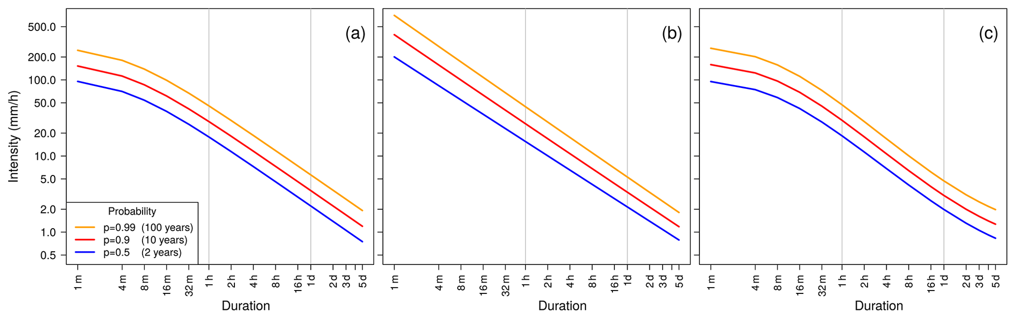
Figure 2 IDF curve examples showing the visualization of different IDF curve features. (a) Curvature for short durations. (b) Multiscaling. (c) Curvature for short durations, flattening for long durations, and multiscaling.

When applying the GEV separately to every duration out of a set of durations and interpolating in a second independent modeling step, the number of parameters equals three GEV parameters times the number of selected durations plus at least three parameters for interpolating every quantile. For the set of durations chosen here, and for evaluating five quantiles, this implies estimating 15 × 3 + 5 × 3 = 60 parameters. For the consistent approach, estimation is reduced to only five d-GEV parameters, i.e., $\stackrel{\mathrm{̃}}{\mathit{\mu }}$, σ₀, ξ, θ, and η. A smaller parameter set is less likely to overfit the data and enables us to better investigate underlying physical processes.

Models can be further improved by adding the multiscaling feature (Gupta and Waymire, 1990; Burlando and Rosso, 1996; Van de Vyver, 2018) which introduces different slopes, depending on the quantile (or associated probability). Figure 2b presents how this feature affects the IDF curves. In order to highlight the effect of the multiscaling, we set θ=0, resulting in no deviation from a power law (curvature) for short durations. The multiscaling feature is added at the cost of one additional parameter η₂ (second duration exponent) in the model, as follows:

$$\begin{array}{}\text{(8)}& {\displaystyle }\mathit{\sigma }\left(d\right)& {\displaystyle }={\mathit{\sigma }}_{\mathrm{0}}{d}^{-(\mathit{\eta }+{\mathit{\eta }}_{\mathrm{2}})}\text{(9)}& {\displaystyle }\mathit{\mu }\left(d\right)& {\displaystyle }=\stackrel{\mathrm{̃}}{\mathit{\mu }}{\mathit{\sigma }}_{\mathrm{0}}{d}^{-\mathit{\eta }}.\end{array}$$

Using only the curvature feature, Ulrich et al. (2020) reported decreasing performance in consistent modeling for longer durations d≥24 (1 d) when compared to using separate GEV models for each duration. Our attempt aims at more flexibility in the IDF curve in the long-duration regime. Therefore, we combine both features, curvature (duration offset) and multiscaling (second duration exponent), and add a new parameter τ, the intensity offset, which allows for a slower decrease of intensity for very long durations d≫24 (Fig. 2c). This effect will be called flattening in the following:

$$\begin{array}{}\text{(10)}& {\displaystyle }\mathit{\sigma }\left(d\right)& {\displaystyle }={\mathit{\sigma }}_{\mathrm{0}}(d+\mathit{\theta }{)}^{-(\mathit{\eta }+{\mathit{\eta }}_{\mathrm{2}})}+\mathit{\tau },\text{(11)}& {\displaystyle }\mathit{\mu }\left(d\right)& {\displaystyle }=\stackrel{\mathrm{̃}}{\mathit{\mu }}\left({\mathit{\sigma }}_{\mathrm{0}}\right(d+\mathit{\theta }{)}^{-\mathit{\eta }}+\mathit{\tau }).\end{array}$$

Summarizing this section, the following three different features were presented: (1) curvature, described by the duration offset parameter θ, (2) multiscaling, using a second duration exponent η₂, and (3) flattening with the intensity offset τ, which is introduced in this study. In the following, we use the notation IDF_c for a model including only the curvature feature, i.e., η₂=0 and τ=0, IDF_m for a model including only the multiscaling feature, i.e., θ=0 and τ=0, and IDF_f for a model including only the flattening feature, i.e., θ=0 and η₂=0. Feature combinations are denoted as, e.g., IDF_cmf for all features. The plain duration-dependent model without curvature, multiscaling, and flattening is denoted as IDF.

2.4 Parameter estimation

Parameters of the d-GEV distribution are estimated by maximizing the likelihood (maximum likelihood estimation – MLE) under the assumption of independent annual maxima. Jurado et al. (2020) showed that independence is a reasonable assumption in many cases, especially for long durations. Their study was performed on an earlier version of the same data set that was used in this study. Moreover, Rust (2009) showed that in strongly dependent time series convergence towards the GEV distribution is slower. But, assuming an appropriate choice of model, dependence does not play a large role. We use the negative log-likelihood L, to avoid using products of small numbers, as follows:

$$\begin{array}{}\text{(12)}& \begin{array}{rl}& L(\stackrel{\mathrm{̃}}{\mathit{\mu }},{\mathit{\sigma }}_{\mathrm{0}},\mathit{\xi },\mathit{\theta },\mathit{\eta },{\mathit{\eta }}_{\mathrm{2}},\mathit{\tau }\mid Z)\\ & =\sum _{n=\mathrm{1}}^N\sum _{d\in D}-\log \left(G(z_{n,d},d\mid \stackrel{\mathrm{̃}}{\mathit{\mu }},{\mathit{\sigma }}_{\mathrm{0}},\mathit{\xi },\mathit{\theta },\mathit{\eta },{\mathit{\eta }}_{\mathrm{2}},\mathit{\tau })\right),\end{array}\end{array}$$

with the number of data points N, the duration set D, data points for each duration z_n,d, and the characteristic parameters of the modified d-GEV $\stackrel{\mathrm{̃}}{\mathit{\mu }},{\mathit{\sigma }}_{\mathrm{0}},\mathit{\xi },\mathit{\theta },\mathit{\eta },{\mathit{\eta }}_{\mathrm{2}},\mathit{\tau }$. The sum of L over all data points Z is minimized with the R package optim() function (R Core Team, 2020). The R package IDF (Ulrich et al., 2021b), which was already used for the accumulation, also provides functions for fitting and plotting IDF curves. Its functionality was extended in the context of this study and now provides options for both multiscaling and flattening in IDF curves.

Finding reasonable initial values for d-GEV parameters in the optimization process was a major challenge during parameter estimation because optimization stability strongly depends on the choice of initial values. Details about this procedure can be found in Appendix A.

2.5 Quantile skill index

After estimating GEV parameters, quantiles q (return levels) can be predicted for a chosen non-exceedance probability p (or return period T, with $T=\mathrm{1}/(\mathrm{1}-p)$), using Eq. 3. To verify how well a modeled quantile q of a given probability p represents extremes in the data, we use the quantile score (QS) as follows (Koenker and Machado, 1999; Bentzien and Friederichs, 2014):

$$\begin{array}{}\text{(13)}& \text{QS}\left(p\right)=\sum _n^N{\mathit{\rho }}_{\mathrm{p}}(z_n-q),\end{array}$$

with a small score indicating a good model. Here, ρ_p is the tilted absolute value function, also known as the so-called check function.

$$\begin{array}{}\text{(14)}& {\mathit{\rho }}_{\mathrm{p}}\left(u\right)=\left\{\begin{array}{ll}pu& ,u>\mathrm{0}\\ (p-\mathrm{1})u& ,u\le \mathrm{0},\end{array}\right.\end{array}$$

with $u=z_n-q$. For high non-exceedance probabilities p, it leads to a strong penalty for data points that are still higher than the modeled quantile (z_n>q). Using this approach, the QS allows for detailed verification for each probability p and duration d separately by predicting a quantile intensity for a given p and d and comparing it with data points z_n,d of duration d.

To compare different IDF models in terms of the QS, we require another verification measure. The quantile skill score QSS compares the quantile score QS_M of a new IDF model M with the quantile score QS_R of a reference IDF model R as follows:

$$\begin{array}{}\text{(15)}& {\text{QSS}}_{M\mid R}=\mathrm{1}-{\text{QS}}_M/{\text{QS}}_R.\end{array}$$

The QSS takes values $-\mathrm{\infty }<\text{QSS}\le \mathrm{1}$ with QSS=1 for a perfect model. Positive values ${\text{QSS}}_{M\mid R}>\mathrm{0}$ are associated with an improvement of M over R. In case the model M is outperformed by the reference R, the resulting QSS is negative ${\text{QSS}}_{M\mid R}<\mathrm{0}$. In this case, its value is not easily interpretable. This issue is acknowledged by the quantile skill index (QSI) suggested by Ulrich et al. (2020). In the case of ${\text{QSS}}_{M\mid R}<\mathrm{0}$, reference R and model M are exchanged and $-{\text{QSS}}_{R\mid M}$ is used for negative values of the QSI, as follows:

$$\begin{array}{}\text{(16)}& \text{QSI}=\left\{\begin{array}{ll}\mathrm{1}-{\text{QS}}_M/{\text{QS}}_R& ,{\text{QS}}_M\le {\text{QS}}_R\\ {\text{QS}}_R/{\text{QS}}_M-\mathrm{1}& ,{\text{QS}}_M>{\text{QS}}_R.\end{array}\right.\end{array}$$

The QSI has a symmetric range and indicates either (1) a good skill over the reference when leaning clearly towards 1, (2) little or no skill when being close to 0, or (3) worse performance than the reference when leaning clearly towards −1.

In this study, the quantile score was calculated in a cross-validation setting. For each station, the available years with maxima are divided into n_cv non-overlapping blocks of 3 consecutive years. Then, for each cross-validation step i, one block is chosen as testing set, and all the other blocks are used as training data set. For the remaining cross-validation steps, this procedure is repeated with another block chosen as testing set in each step until all blocks have been used as testing sets exactly once. The cross-validated QS is obtained by averaging the score of all cross-validation steps as follows:

$$\begin{array}{}\text{(17)}& {\text{QS}}^{\text{cv}}={\displaystyle \frac{\mathrm{1}}{n_{\text{cv}}}}\sum _{i=\mathrm{1}}^{n_{\text{cv}}}{\text{QS}}_i.\end{array}$$

Then, the QSI is derived from the averaged cross-validated QS of the model, ${\text{QS}}_M^{\text{cv}}$, and the averaged cross-validated QS of the reference, ${\text{QS}}_R^{\text{cv}}$, according to Eq. (16). If a year was assigned to the training or testing data set, then all available accumulation durations are used for training or testing, respectively, to avoid dependence between the test and validation set.

In order to compare individual model features, we will use the mentioned models without this specific feature as a reference in the following.

2.6 Bootstrapping and coverage

To provide an estimate of the uncertainty of the intensity quantile estimates in IDF curves, we obtain 95 % confidence intervals using a bootstrapping method. To account for dependence between annual maxima of different durations, we apply the ordinary non-parametric bootstrap percentile method (Davison and Hinkley, 1997) as follows.

Please note that, in this paragraph, the empirical quantiles used for the confidence intervals should not be confused with the intensity quantiles, which describe the return level and are referred to as quantiles as well. For each station, we draw a sample of years (with replacement) from the set of years with available data. This way, for a chosen year, all maxima from this year are used, and we expect that sampling in this way maintains the dependence structure of the data. We then estimate the parameters of the d-GEV, which is used to calculate the intensity quantile that is connected to a certain non-exceedance probability (see Eq. 3). We obtain a distribution of the estimated intensity quantiles by repeating this process 500 times. From this distribution, we use the empirical 0.025 and 0.975 quantiles to obtain the upper and lower bounds of the 95 % confidence interval of intensity quantiles.

We conduct a simulation study to examine whether the derived confidence intervals provide reasonable coverage despite the dependence between the annual maxima of different durations. Therefore, we simulate 500 samples of data, each with a size of n = 50 years, with a known dependence between durations. In a first case, samples with no dependence between durations are obtained by drawing random values from a d-GEV distribution. Further details on the simulated data can be found in Appendix Sect. B. In a second case, to obtain data with dependence between durations, we use the R package SpatialExtremes to simulate values from a Brown–Resnick simple max-stable process with known dependence parameters. We use the range and smooth parameter $(\mathit{\rho },\mathit{\alpha })\in \mathit{\left\{}\right(\mathrm{1},\mathrm{0.2}),(\mathrm{120},\mathrm{1}),(\mathrm{60},\mathrm{1}\left)\mathit{\right\}}$ for (1) a weak dependence, (2) a strong dependence, and (3) a dependence found for Wupper catchment (Jurado et al., 2020), respectively. We transform the simulated data from having Fréchet margins to d-GEV margins with the chosen parameters, as done by Jurado et al. (2020), and adjust them to the hourly scale used in this study. Then, for the artificial data, confidence intervals are obtained by bootstrapping with 500 repetitions, as described above. For better understanding, this results in a total of 500 × 500 × 50 data points and 500 confidence intervals. The ratio of samples in which the confidence intervals cover the true intensity z and the total number of samples (500) is called the coverage. It can be calculated for each duration and probability separately.

3 Results

Results are presented in the following order: (1) modeling performance is verified with the QSI for the three different IDF curve features, i.e., curvature, multiscaling, and flattening. (2) IDF curves with all three features are shown for two rain gauges. Curves are presented with a 95 % confidence interval, as created by a bootstrapping method. (3) The trustworthiness of this bootstrapping method applied to the new model with all three features is investigated with a coverage analysis, based on simulated data.

3.1 Model validation

The QSI is used to compare the quantile score of a model with that of a reference. In order to specifically investigate the influence of a single model feature, we use these features in a model and compare with a reference without this specific feature; e.g., ${\text{QSI}}_{{\text{IDF}}_c\mid \text{IDF}}$ gives the performance for a model including only curvature against the plain reference without curvature, or ${\text{QSI}}_{{\text{IDF}}_{\text{cmf}}\mid {\text{IDF}}_{\text{mf}}}$ gives the performance for the full model including curvature, multiscaling, and flattening against a reference with multiscaling and flattening and without curvature (see Sect. 2.3).

Figure 3 shows the QSI for an IDF model including each of the three features of curvature, multiscaling, and flattening (columns) combined with no other, one other, or both other features (rows) against a reference model which differs only in the one feature under investigation (labels on top of the columns). For each ${\text{QSI}}_{{\text{IDF}}_{\mathrm{1}}\mid {\text{IDF}}_{\mathrm{2}}}$, one panel is provided in Fig. 3. Models and references are listed in Table E1 in Appendix. E. In this way, the potential performance of each feature, e.g., curvature, is analyzed and is denoted as e.g., curvature skill. QSI values between −0.05 and 0.05 are considered as being an indicator of no relevant difference between model performances.

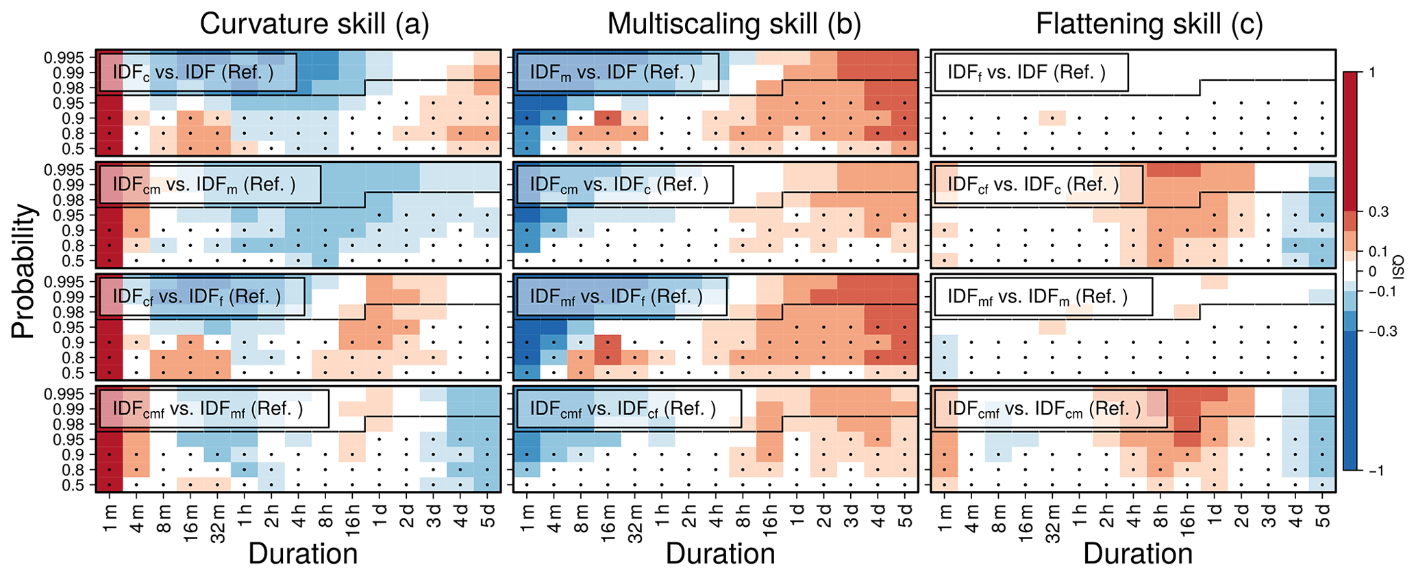
Figure 3 Quantile skill index (QSI) of the three features (columns) for four different cases (rows) where the investigated feature is combined with no other (upper row), one other (second and third row), or both other features (lower row) in model and reference. Column titles indicate the feature switched on in the model and switched off in the reference. The slightly opaque labels in the panels indicate which model and reference is used (see also Table E1). Dots show whether the average length of the time series over all stations is longer than the return period $T=\mathrm{1}/(\mathrm{1}-p)$ (here shown as probability p) and indicate the verification trustworthiness. Black lines are derived from the number of years of the station with the longest time series. The verification for rare events (upper part of each panel) above the black line has to be treated carefully because the data do not cover this time period. For this verification plot, only stations that provide data on a minute scale were used.

The curvature (duration offset θ≠0) for short durations can be explained by a stronger connection between the annual maxima of different durations, which tend to originate from the same event. Usually, the most intense phase of a heavy precipitation event lasts for several minutes, and aggregated maxima do not differ much on this scale. Based on this idea, curvature influences the IDF curve's shape only for very short durations below 1 h (Fig. 2a). The consistently positive QSI values for $d=\mathrm{1}/\mathrm{60}$ (1 min) for the curvature skill support this theory. These results show that this duration regime $d=\mathrm{1}/\mathrm{60}$ is much better modeled with the curvature, compared to models without this feature. However, the slope for medium durations, described by the duration exponent (see Fig. 2b), is steeper when using curvature compared to models that do not use curvature. So, for medium and long durations, models perform equally well or worse when curvature is used than reference models without curvature, in most cases, on average (see the blue regimes in Fig. 3a). In the absence of multiscaling (rows 1 and 3), a further performance increase could be found for durations between 8 h and 5 d.

Multiscaling allows for different slopes of different p quantiles on a double logarithmic scale. Figure 3b shows that this feature increases modeling performance mainly for long, but also for some sub-hourly, durations when estimating quantiles for small non-exceedance probabilities. Not using curvature enables a small multiscaling skill gain for sub-hourly durations (rows 1 and 3 in Fig. 3b). An explanation could be that multiscaling tends to let IDF curves associated with different return periods diverge for short durations and converge for long durations. This behavior might interfere with the duration offset's introduction of curvature in short durations. Furthermore, the presence of curvature leads to a slightly smaller skill increase for durations longer than 16 h (rows 2 and 4 in Fig. 3b). This effect agrees with the results from the curvature skill verification (Fig. 3a), where it was shown that curvature improves modeling performance only for very short durations and has no or a negative effect on medium and long durations.

The intensity offset τ is a new feature, first introduced in this study, which addresses the empirically observed slower decrease in intensity for very long durations, called flattening. In the case where curvature is enabled in both model and reference (rows 2 and 4 in Fig. 3c), the flattening feature improves modeling performance slightly for the shortest duration of 1 min and strongly for medium durations between 2 h and 1 d. Here, the flattening might compensate for the loss in skill that we observe for medium durations for models with curvature. In these cases, there is a slight loss in skill for very long durations. In cases where curvature is not used, flattening is not needed as it provides no clear skill. An explanation for the flattening of the IDF curves in long durations could be seasonal effects, with annual maxima of short or long durations occurring more often in the summer or winter months, respectively. These effects are currently under further investigation.

When modeling only the durations d≥1 (1 h) of all available stations, the models are rather indifferent towards parameterization (Fig. 4). Here, multiscaling and flattening show some skill improvements for long and medium durations, respectively, similar to that in Fig. 3, but to a much smaller extent when compared to a data set which uses the whole range of durations from 1 min to 5 d for both training and testing (Fig. 3).

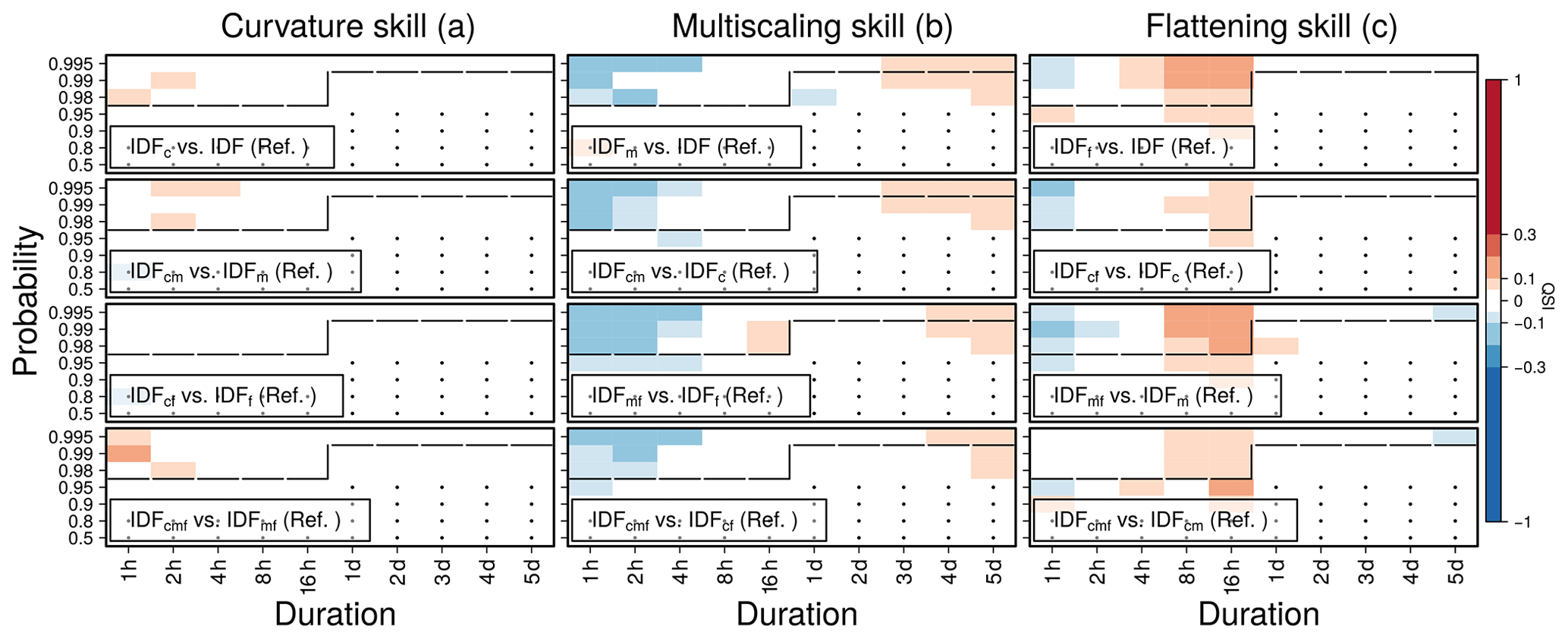
Figure 4 Quantile skill index for data with an hourly resolution. The visualization scheme follows that of Fig. 3. Here, all models were trained and tested for durations d≥1. Here, all stations were considered, regardless of the temporal resolution.

We conclude that the choice of parameters depends on the study purpose. When focusing on long ranges of durations, we recommend using features like curvature, multiscaling, and flattening. If the focus lies on long durations, or the data do not provide a sub-hourly resolution, simple scaling models might be sufficient. These recommendations are further elaborated on in the discussion in Sect. 4.

3.2 IDF curves

Figure 5 shows IDF curves for the stations Bever and Buchenhofen, where a long precipitation series is available (51 years with minute resolution and 76 years with daily resolution in Bever and 19 and 77 years in Buchenhofen, respectively). The difference in available years for different durations has an impact on the width of 95 % confidence intervals, with uncertainty being larger when little data are available. Noticeably, confidence intervals for both stations for p=0.99 and $d=\mathrm{1}/\mathrm{60}$ have a wide range over more than 100 $\mathrm{mm}/\mathrm{h}$. Considering that the 100-year return level was not observed in either station, a wide confidence interval range was expected. For p≤0.8 in Bever, the confidence intervals remain narrow, even on a minute scale.

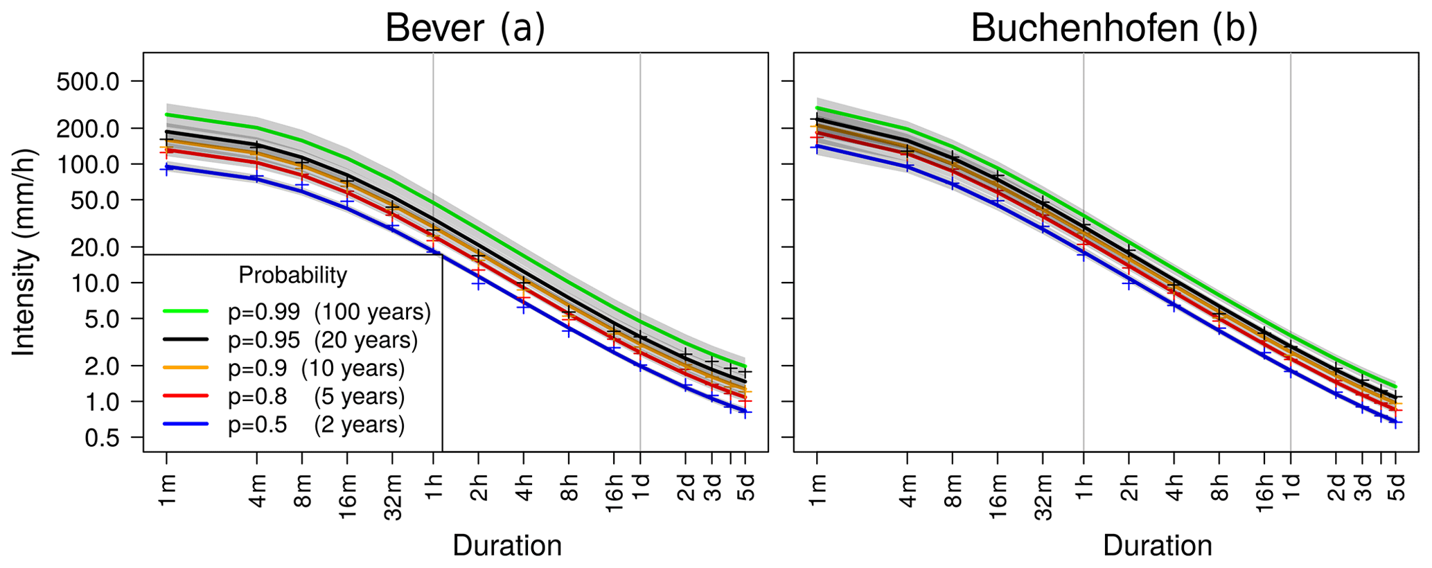
Figure 5 IDF curves for two example stations within the Wupper catchment. Empirical quantile estimates are denoted with the plus signs (+). Confidence intervals are obtained from a bootstrapping procedure.

3.3 Coverage

Confidence intervals in Fig. 5 are obtained from a bootstrapping procedure. In the formulation of the likelihood, we assume the maxima of different durations to be independent. This assumption might not be justified especially for short durations (see  Jurado et al., 2020), and thus, this dependence must be taken into account when estimating uncertainties. Disregarding the dependence would result in an underestimation of the uncertainty. To account for this effect, all annual maxima of each year – for all considered durations – are always included jointly into a bootstrapping sample. We assume that this procedure preserves the dependence structure between durations. To investigate this assumption, we calculate the coverage of simulated data (see Appendix B) from (1) a d-GEV distribution without dependence and a Brown–Resnick max-stable process with (2) a typical dependence for the Wupper station (Jurado et al., 2020) and (3) a rather weak and (4) strong dependence between durations (Fig. 6). In the first case without any dependence, the displayed coverage does completely agree with the 95 % confidence interval, without any respect to duration or frequency (probability). When using dependence on a weak or strong level, the coverage is smaller but still around 90 %. This can be interpreted as an underestimation of uncertainty, to a small extent, by the confidence intervals in the case of a high dependence. The true dependence of durations was not investigated in this study and could be lower. That said, these results suggest that bootstrapping is a suitable tool for estimating confidence intervals in the presented context.

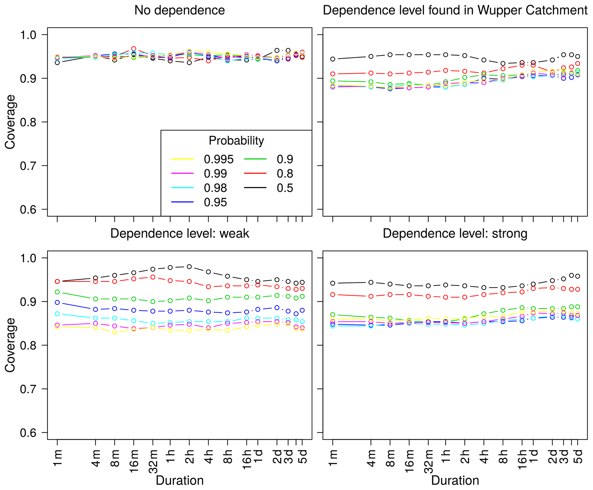
Figure 6 Bootstrapping coverage. Using a Brown–Resnick max-stable process, the coverage was determined in order to investigate the reliability of 95 % confidence intervals from bootstrapping. A total of three different levels of dependence were used.

4 Discussion

In this study, we show that model performance can be increased when the flattening of IDF curves in the long-duration regime is taken into account. We assume that this behavior arises from seasonal effects. That means that the annual maxima of different durations may not follow the same scaling process. However, this topic is currently under further investigation (Ulrich et al., 2021a).

The analyzed features – curvature, multiscaling, and flattening – were seen in the results to have a different impact on modeling performance, depending on the duration and return period. All features are able to improve the model for certain regimes, but depending on the problem that is approached, features should be chosen accordingly. If the focus is on a small timescales of minutes, then the curvature skill is important for a good modeling result. When curvature is used and medium to long timescales are also of importance, then the flattening feature should be used. This helps to compensate for the deterioration due to curvature over longer durations. Multiscaling is a good choice if a loss in skill for short durations can be accepted in exchange for a simultaneous improvement at long durations, regardless of which other features are requested.

The skills of the features depend on another feature's presence. This dependence is strongest for the flattening, which can only improve the model when curvature is used. The modeling performance of the curvature depends less on the presence of other features. The same applies to the multiscaling feature.

These suggestions hold for models that are supposed to cover a wide range of timescales from minutes to days. For data with hourly or more coarse temporal resolution, the skill gain from using the features is much smaller. Here, flattening can improve the model slightly on a daily timescale and multiscaling only improves modeling long durations a little bit but leads to a slight reduction in skill for the hourly timescale.

Additional parameters give the model more flexibility. Including τ in the model allows one to reduce deviations between model and data points particularly for long durations. This, in turn, opens the possibility to vary the remaining parameters such that deviations between model and data points can be reduced in other (e.g., short) duration regimes. Conversely, this also holds when including θ. In this way, a parameter that changes the curve in long durations can increase the modeling performance in other durations and even slightly decrease model performance in long durations in certain cases. In Fig. 7, IDF curves for two models are compared for a chosen station (Bever). The model that includes flattening (IDF_cmf) is able to follow the empirical quantiles in long durations as well as the model without flattening (IDF_cm). However, flattening gives the model the opportunity to better follow the empirical quantiles in medium durations between 4 h and 1 d, which is in accordance with the results in Fig. 3c.

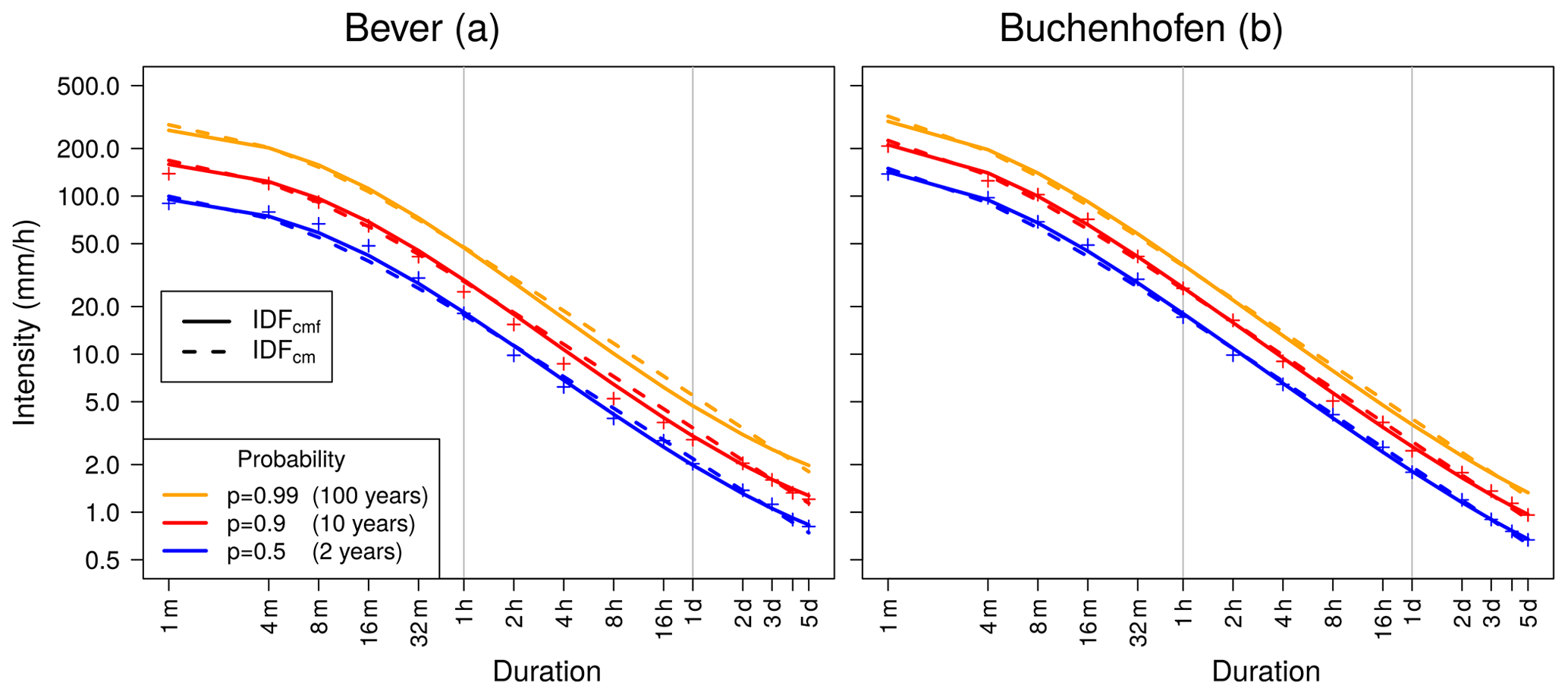
Figure 7 IDF curve for Bever. A comparison of a model with flattening (IDF_cmf) and a model without flattening (IDF_cm). Empirical quantile estimates are denoted with the plus signs (+).

The parametric form of the IDF relation is based on three modifications to a simple power law which are motivated by our understanding of the rainfall process, namely curvature (e.g., Koutsoyiannis et al., 1998) for small durations addressing limits to rainfall intensity, multiscaling (e.g., Van de Vyver, 2018) taking care of a varying scaling behavior for events of different strength, and flattening (suggested here) resulting from a mixing of convective and stratiform generated precipitation extremes from different seasons in the climate regime under study. Our contribution is to combine these modifications into a flexible parametric form capable of describing various effects related to rainfall processes. The resulting model is based on empirical grounds, and it can be shown to improve the description over simple power law models. Other modifications are possible. To our knowledge, there is no theoretical justification for these forms which can be derived from first principles for rainfall processes. Since our results might apply only to the geographical region under investigation, further studies are necessary to find out whether the found model performances of the different features are generally applicable. The character of the shape parameter ξ with respect to duration is still unclear, since no linear or log-linear duration dependence could be found as with the location and scale parameters μ and σ. A possible approach would be to let the shape parameter vary smoothly across durations in a non-parametric manner but to penalize its deviation from the median over all durations (Bücher et al., 2021). However, the scarce data availability hampers a more complex estimation of the shape parameter.

5 Summary and outlook

The aim of this study is to compare and suggest new parametric forms of consistent IDF curves that are applicable to a large range of durations from minutes to several days and, therefore, cover events from short-lived convective storms to long-lasting synoptic events. The dependence on duration is implemented in the location and scale parameter and allows for three features, i.e., curvature, multiscaling, and flattening. The analysis of these features enables us to understand more about the underlying physical effects beyond the subject of return periods and provides more flexible IDF curves that are suitable for a wide range of durations. The results of our simulation study show that we are able to provide reasonable estimates of uncertainty using bootstrapping and also with regard to dependence between durations.

Our findings agree with Veneziano and Furcolo (2002), who found that simple scaling was adequate for modeling short durations, and multiscaling was adequate for long durations. Moreover, our conclusion that curvature improves the modeling of short durations indirectly agrees with Bougadis and Adamowski (2006), who used different slopes for durations longer or shorter than 1 h, respectively, and concluded that linear scaling does not hold for small durations.

Consistent modeling using the d-GEV enables the use of fewer parameters. In this way, the model can be easily extended, e.g., using physically relevant atmospheric covariates. Thus, improving the parameterization of the d-GEV is crucial to leading the path for further steps. In future studies, we plan to include spatial covariates into the estimation of the newly proposed d-GEV parameters, including intensity offset, in order to use data from different locations more efficiently. Also, the concept of non-stationary precipitation with respect to IDF curves is important to consider (see Cheng and AghaKouchak, 2014; Ganguli and Coulibaly, 2017; Yan et al., 2021) since extremes are expected to vary due to climate change. For example, Benestad et al. (2021) found a model that enables downscaling of 24 h measurement data to shorter durations without assuming stationarity. However, we think that implementing atmospheric large-scale covariates (as in Agilan and Umamahesh, 2017) into the flexible d-GEV model proposed here would allow for a better understanding of the underlying processes. We plan to use this approach to investigate the change in characteristics of extreme precipitation due to climate change in future studies. While the choice of method depends on the study target, different approaches have been taken to create IDF curves, as in Bezak et al. (2016), who used copula-based IDF curves and reported that IDF curves might be sensitive to the choice of method. This is important to consider when deciding on the appropriate way to create IDF curves. Moreover, the origin of flattening in annual maxima for long durations is currently investigated in more detail (Ulrich et al., 2021a).

The analysis of the performance shows that the new parametric form of the duration-dependent GEV suggested here, together with the bootstrap-based confidence intervals, offers a consistent, flexible, and powerful approach to describing the intensity–duration–frequency (IDF) relationships for various applications in hydrology, meteorology, and other fields.

Appendix A: Initial values

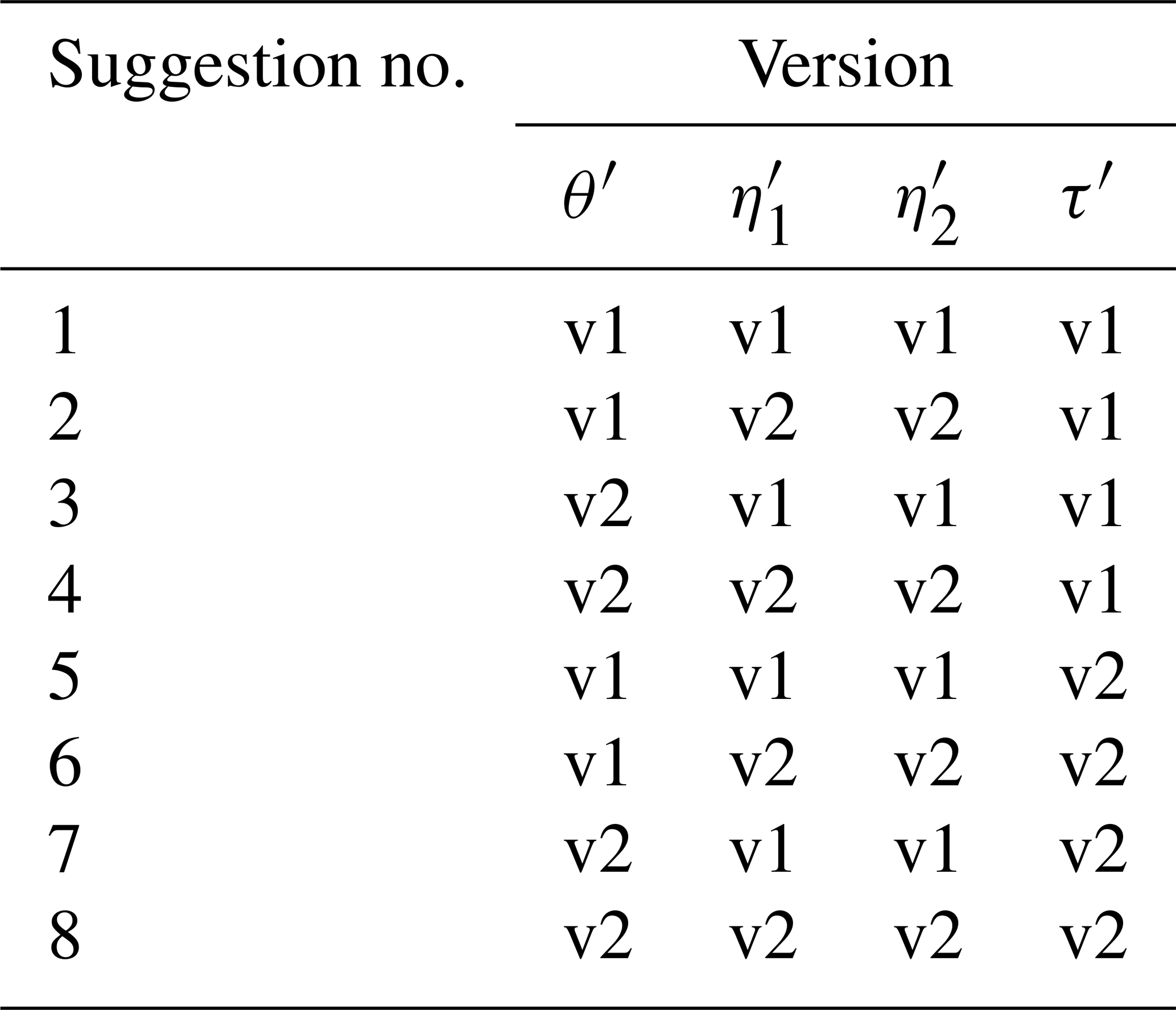
The estimation of d-GEV parameters was conducted with the R base optim() function (R Core Team, 2020) and the Nelder–Mead method. The quality of the fitted model depends on the initial values passed to the function. Each optimization i was repeated m times with different initial values that are derived through different techniques. The sets of initial functions, i.e., $s_i\in \mathit{\{}{\stackrel{\mathrm{̃}}{\mathit{\mu }}}^{\prime },{\mathit{\sigma }}_{\mathrm{0}}^{\prime },{\mathit{\xi }}^{\prime },{\mathit{\theta }}^{\prime },{\mathit{\eta }}^{\prime },{\mathit{\eta }}_{\mathrm{2}}^{\prime },$ and τ^′}, were collected as suggestions, and the individual parameters were named with version indices (v1, v2, etc.). All suggestions were subsequently used as initial values in the model, and the suggestion which led to the smallest negative log likelihood was selected. Table A1 gives an overview of the combinations of initial values.

All initial-value techniques were based on the same first step. An individual GEV distribution was fitted to each duration d separately, with moment estimators as initial values (Coles, 2001), and the three GEV parameters of location μ, scale σ, and shape ξ were stored for each duration. In the next step, a function was fitted to each of the parameters with respect to the duration. Since we assumed no dependence of the shape parameter on the duration, we chose ${\mathit{\xi }}_{\text{v1}}^{\prime }=\text{median}\left(\mathit{\xi }\right)$ for all suggestions. According to Eqs. (4) and (5), we fitted log (σ(d)) and log (μ(d)) as a function of log (d) in a linear regression with a simple slope and y intercept as follows:

$$\begin{array}{}\text{(A1)}& {\displaystyle }\log \left(\mathit{\sigma }\right(d\left)\right)& {\displaystyle }\sim -(\mathit{\eta }+{\mathit{\eta }}_{\mathrm{2}})\log \left(d\right)+\log \left({\mathit{\sigma }}_{\mathrm{0}}\right)\text{(A2)}& {\displaystyle }\log \left(\mathit{\mu }\right(d\left)\right)& {\displaystyle }\sim -\mathit{\eta }\log \left(d\right)+\left(\log \right({\mathit{\sigma }}_{\mathrm{0}})+\log (\stackrel{\mathrm{̃}}{\mathit{\mu }}\left)\right),\end{array}$$

with given σ(d), μ(d), and d. From this fit, we extracted ${\mathit{\sigma }}_{\mathrm{0},\text{v1}}^{\prime }=\exp \left(\log \right({\mathit{\sigma }}_{\mathrm{0}}\left)\right)$ (Eq. A1), ${\stackrel{\mathrm{̃}}{\mathit{\mu }}}_{\text{v1}}^{\prime }=\stackrel{\mathrm{̃}}{\mathit{\mu }}$ (combine Eqs. A1 and A2), ${\mathit{\eta }}_{\text{v1}}^{\prime }=\mathit{\eta }$, and ${\mathit{\eta }}_{\mathrm{2},\text{v1}}^{\prime }={\mathit{\eta }}_{\mathrm{2}}$. For the most simple suggestion of initial parameters, we chose ${\mathit{\theta }}_{\text{v1}}^{\prime }=\mathrm{0}$ and ${\mathit{\tau }}_{\text{v1}}^{\prime }=\mathrm{0}$. In the next steps, we further elaborated the ways of finding good initial values. Version 2 of the duration exponents ${\mathit{\eta }}_{\text{v2}}^{\prime }$ and ${\mathit{\eta }}_{\mathrm{2},\text{v2}}^{\prime }$ were found, using only d≥ 1 h, because the slope is mainly characterized by this duration regime. This is the second set of suggestions for initial values, together with version 1 of the other parameters.

Another initial duration offset ${\mathit{\theta }}_{\text{v2}}^{\prime }$ could be estimated by fitting a nonlinear squares regression (R function nls) as follows:

$$\begin{array}{}\text{(A3)}& {\displaystyle }\log \left(\mathit{\sigma }\right(d\left)\right)& {\displaystyle }\sim -(\mathit{\eta }+{\mathit{\eta }}_{\mathrm{2}})\log (d+\mathit{\theta })+\log \left({\mathit{\sigma }}_{\mathrm{0}}\right)\text{(A4)}& {\displaystyle }\log \left(\mathit{\mu }\right(d\left)\right)& {\displaystyle }\sim -\mathit{\eta }\log (d+\mathit{\theta })+\log \left({\mathit{\sigma }}_{\mathrm{0}}\stackrel{\mathrm{̃}}{\mathit{\mu }}\right),\end{array}$$

with given σ(d), μ(d), and d. The mean of both estimates for θ was used for ${\mathit{\theta }}_{\text{v2}}^{\prime }$. These functions were less stable and provided worse initial values for ${\mathit{\sigma }}_{\mathrm{0}}^{\prime }$ and ${\stackrel{\mathrm{̃}}{\mathit{\mu }}}^{\prime }$ than Eqs. (A1) and (A2). That is why we used them only for estimating initial ${\mathit{\theta }}_{\text{v2}}^{\prime }$ in the nls function and not for estimating initial $\stackrel{\mathrm{̃}}{\mathit{\mu }}$, σ₀, η₁, or η₂. The new initial estimate ${\mathit{\theta }}_{\text{v2}}^{\prime }$ was combined with ${\mathit{\eta }}_{\text{v1}}^{\prime }$ and ${\mathit{\eta }}_{\mathrm{2},\text{v1}}^{\prime }$ in one set (suggestion 3) and with ${\mathit{\eta }}_{\text{v2}}^{\prime }$ and ${\mathit{\eta }}_{\mathrm{2},\text{v2}}^{\prime }$ in another set (suggestion 4).

The same nls function was used for an estimation of the initial ${\mathit{\tau }}_{\text{v2}}^{\prime }$, taking only d≥ 1 h and no duration offset (curvature), as follows:

$$\begin{array}{}\text{(A5)}& {\displaystyle }\log \left(\mathit{\sigma }\right(d\left)\right)& {\displaystyle }\sim \log ({\mathit{\sigma }}_{\mathrm{0}}{d}^{-(\mathit{\eta }+{\mathit{\eta }}_{\mathrm{2}})}+\mathit{\tau })\text{(A6)}& {\displaystyle }\log \left(\mathit{\mu }\right(d\left)\right)& {\displaystyle }\sim \log ({\mathit{\sigma }}_{\mathrm{0}}\stackrel{\mathrm{̃}}{\mathit{\mu }}{d}^{-\mathit{\eta }}+\mathit{\tau }),\end{array}$$

with given σ(d), μ(d), and d. Again, the mean of both estimates of τ was used as ${\mathit{\tau }}_{\text{v2}}^{\prime }$. To define suggestions 5–8, this second version of τ^′ was combined with ${\mathit{\theta }}_{\text{v1}}^{\prime }$, ${\mathit{\eta }}_{\text{v1}}^{\prime }$, ${\mathit{\eta }}_{\mathrm{2},\text{v1}}^{\prime }$ or ${\mathit{\theta }}_{\text{v1}}^{\prime }$, ${\mathit{\eta }}_{\text{v2}}^{\prime }$, ${\mathit{\eta }}_{\mathrm{2},\text{v2}}^{\prime }$ or ${\mathit{\theta }}_{\text{v2}}^{\prime }$, ${\mathit{\eta }}_{\text{v1}}^{\prime }$, ${\mathit{\eta }}_{\mathrm{2},\text{v1}}^{\prime }$ or ${\mathit{\theta }}_{\text{v2}}^{\prime }$, ${\mathit{\eta }}_{\text{v2}}^{\prime }$, and ${\mathit{\eta }}_{\mathrm{2},\text{v2}}^{\prime }$. The different combinations of initial value versions are listed again in Table A1.

Table A1 Overview of initial value combinations (suggestions). The initial values for the parameters ${\stackrel{\mathrm{̃}}{\mathit{\mu }}}_{\text{v1}}^{\prime }$, ${\mathit{\sigma }}_{\mathrm{0},\text{v1}}^{\prime }$, and ${\mathit{\xi }}_{\text{v1}}^{\prime }$ are the same in all combinations.

Appendix B: Simulated data

For the coverage analysis in Sect. 3.3 and Appendix C about duration sample choice, we did not use the original data set but simulated data from a d-GEV distribution. The simulated data were drawn, according to Eqs. (3), (10), and (11), with a random number $\mathrm{0}<p<\mathrm{1}$ and the parameters $\stackrel{\mathrm{̃}}{\mathit{\mu }}=\mathrm{3.2}$, σ₀=5.8, ξ=0.21, θ=0.089, η=0.78, η₂=0.09, and τ=0.10. These values were based on realistic parameter values from station data, fitted for the features of curvature, multiscaling, and flattening. When disabling one or more of the features, the values of all the parameters will change. For the coverage analysis, the true quantile intensity z could be calculated directly, using these parameters and Eqs. (3), (10), and (11).

Appendix C: Influence of duration sample choice

We investigate how the choice of durations that are used to train the model influences the model performance. Since the number of training data points is much higher for long durations d≥24 (1 d), there is a possibility that these duration regimes are overrepresented in the training phase, and thus, model performance is worse for short durations. To account for this effect, the model is trained twice (1) with simulated maxima (Appendix B) and the set of aggregated durations that was used for analysis in this study (Eqs. 1 and 2) with simulated annual maxima of a different set of durations that focuses more on short durations (numerically in hours), as follows:

$$\begin{array}{}\text{(C1)}& \begin{array}{rl}& d_{\mathrm{2}}\in \mathit{\{}\mathrm{1},\mathrm{2},\mathrm{3},\mathrm{\dots },\mathrm{15},\mathrm{16},\mathrm{18},\mathrm{20},\mathrm{\dots },\mathrm{30},\mathrm{32},\mathrm{33},\mathrm{36},\mathrm{39},\mathrm{\dots },\\ & \mathrm{57}\min ,\mathrm{1},\mathrm{2},\mathrm{3},\mathrm{\dots },\mathrm{6},\mathrm{8},\mathrm{10},\mathrm{12},\mathrm{15},\mathrm{16},\mathrm{18},\mathrm{21}\mathrm{h},\mathrm{1},\mathrm{3},\mathrm{5}\mathrm{d}\mathit{\}}.\end{array}\end{array}$$

In this way, there is more training data for short durations available, which might shift the model's performance focus to other duration regimes. However, it is important to note that this is only an artificial increase in available data, since the additional data points do not contain substantial new information.

The model with the new artificial training data set (Eq. C1) is now verified against the same model with the previously used artificial data set (Eq. 1) with the following results: all QSIs are below 0.05 for all durations d and all quantiles $q\in \mathit{\{}\mathrm{0.5},\mathrm{0.8},\mathrm{0.9},\mathrm{0.95},\mathrm{0.98}$} (not shown). Thus, the results do not indicate that the choice of accumulation duration significantly influences how well the model performs for certain duration regimes.

Appendix D: Model diagnosis

In order to evaluate whether the GEV distribution is an appropriate choice for this analysis, we provide quantile–quantile (QQ) plots (Fig. D1) for the stations of Bever and Buchenhofen, as chosen in Sect. 3.2. While for Buchenhofen all values follow the angle bisecting line, for Bever only a few outlying events, which all correspond to higher quantiles, leave the confidence intervals. However, their number is small compared to the number of shown data points. So, we conclude that the GEV distribution is a suitable assumption in our case.

Figure D1 QQ plots for selected stations. Confidence intervals were obtained by simulating transformed Fréchet distributed values from the model distribution and extracting a 95 % interval.

Appendix E: Overview of reference models for verification

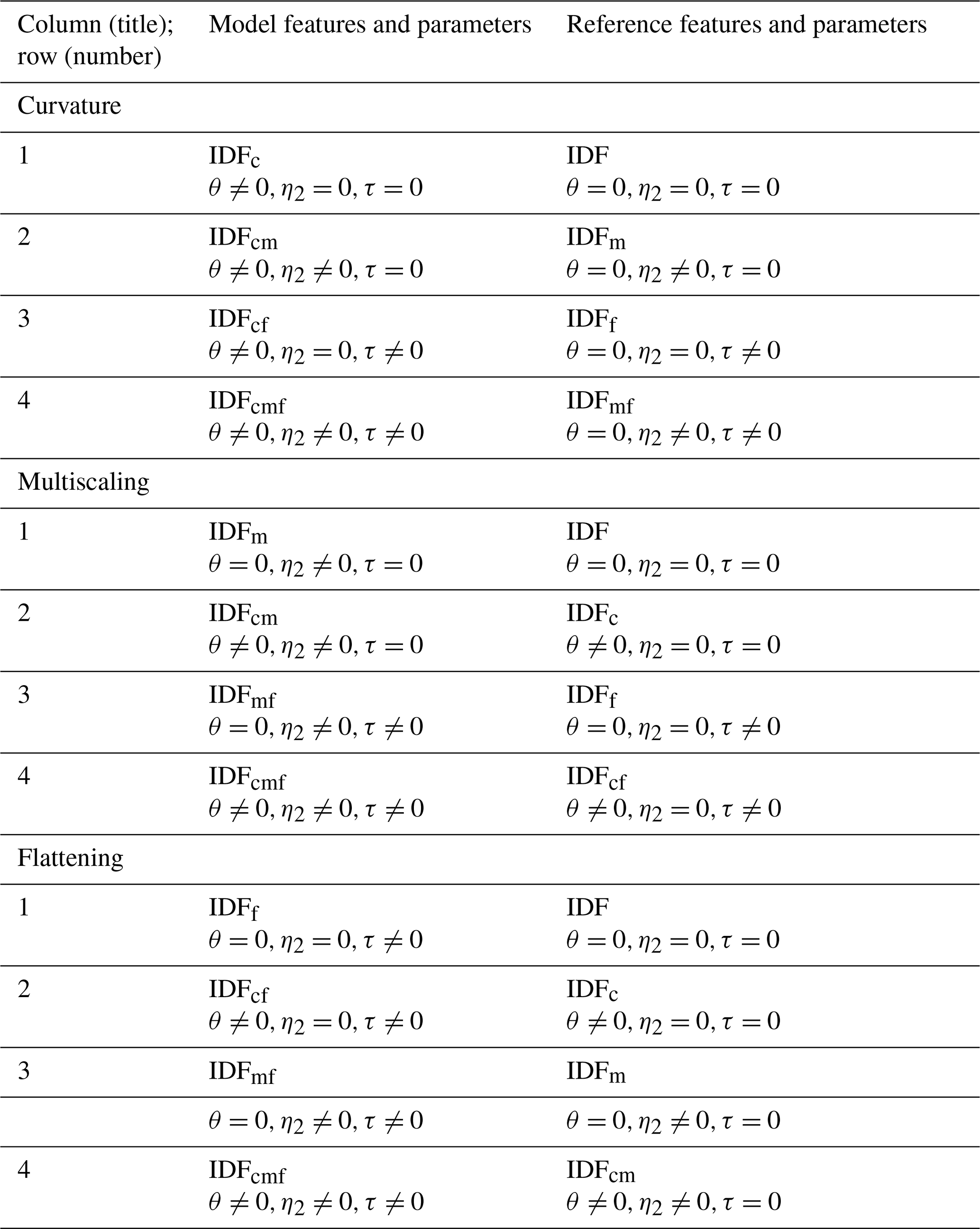
In Sect. 3.1, the feature skill was evaluated by comparing models with a reference where the considered feature is disabled. For clarification, Table E1 lists the models and reference models that were used in Figs. 3 and 4, together with the parameter restriction to zero, if applied. These specifications refer to Eqs. (10) and (11).

Table E1 Overview of models and references for verification.