the Creative Commons Attribution 4.0 License.
the Creative Commons Attribution 4.0 License.
 | 20 Dec 2021
Bending of the concentration discharge relationship can inform about in-stream nitrate removal
Fanny Sarrazin
Rohini Kumar
Jan H. Fleckenstein
Andreas Musolff
Nitrate () excess in rivers harms aquatic ecosystems and can induce detrimental algae growths in coastal areas. Riverine uptake is a crucial element of the catchment-scale nitrogen balance and can be measured at small spatiotemporal scales, while at the scale of entire river networks, uptake measurements are rarely available. Concurrent, low-frequency concentration and streamflow (Q) observations at a basin outlet, however, are commonly monitored and can be analyzed in terms of concentration discharge (C–Q) relationships. Previous studies suggest that steeper positive log (C)–log (Q) slopes under low flow conditions (than under high flows) are linked to biological uptake, creating a bent rather than linear log (C)–log (Q) relationship. Here we explore if network-scale uptake creates bent log (C)–log (Q) relationships and when in turn uptake can be quantified from observed low-frequency C–Q data. To this end we apply a parsimonious mass-balance-based river network uptake model in 13 mesoscale German catchments (21–1450 km2) and explore the linkages between log (C)–log (Q) bending and different model parameter combinations. The modeling results show that uptake and transport in the river network can create bent log (C)–log (Q) relationships at the basin outlet from log–log linear C–Q relationships describing the land-to-stream transfer. We find that within the chosen parameter range the bending is mainly shaped by geomorphological parameters that control the channel reactive surface area rather than by the biological uptake velocity itself. Further we show that in this exploratory modeling environment, bending is positively correlated to percentage of load removed in the network (Lr.perc) but that network-wide flow velocities should be taken into account when interpreting log (C)–log (Q) bending. Classification trees, finally, can successfully predict classes of low (∼4 %), intermediate (∼32 %) and high (∼68 %) Lr.perc using information on water velocity and log (C)–log (Q) bending. These results can help to identify stream networks that efficiently attenuate loads based on low-frequency and Q observations and generally show the importance of the channel geomorphology on the emerging log (C)–log (Q) bending at network scales.
- Article
(6044 KB) - Full-text XML
-
Supplement
(642 KB) - BibTeX
- EndNote


Transport and transformation of nitrate () in river networks are major controls of downstream exports to receiving lakes, reservoirs and coastal systems (Alexander et al., 2000; Billen et al., 1991; Peterson et al., 2001; Seitzinger et al., 2002; Seybold and McGlynn, 2018). Increased concentrations in surface waters can induce detrimental algae growths (Beusen et al., 2016; Canfield et al., 2010; Galloway et al., 1995), compromise river ecosystem health and jeopardize drinking water supplies. Since the beginning of the 20th century, human activities such as agricultural expansion and fossil fuel burning have mobilized additional reactive nitrogen (N), initiating and later exacerbating this problem (Seitzinger et al., 2002). In arable landscapes, which include large parts of Europe, the efficient management of aquatic at network scales is complicated by the spatiotemporal variability in loading patterns and hydrologic regimes as well as the lack of understanding of nutrient pathways, connected transit times and removal processes from input to export. Nevertheless, nitrate concentration and load variability can be predicted at catchment scales when relying on detailed process understanding regarding transport and biogeochemical processing (Alexander et al., 2009; Schlesinger et al., 2006; Wollheim et al., 2008). Moving beyond small-scale variability and characterizing nitrate processing at the catchment scale however remains a challenge (McDonnell et al., 2007; Li et al., 2020).
Within river reaches and streams, reactive solutes like are affected by complex interactions of physical, biological and chemical processes. Physical transport is driven by local discharge and channel geomorphology and dictates the residence time in a reach, thus influencing the timescales at which biogeochemical processing can take place (Kirchner et al., 2000; Runkel and Bencala, 1995; Zarnetske et al., 2011). is removed and transformed by denitrifying bacteria in the anoxic river sediment (Birgand et al., 2007; Peterson et al., 2001); ammonified; or retained through assimilation processes in the oxic or anoxic river compartments by bacteria, fungi and primary producers such as algae and macrophytes, potentially entering higher trophic levels. In the latter case, N in the form of DON (dissolved organic nitrogen) and more commonly DIN (dissolved inorganic nitrogen), together with phosphorus (P), may be released to the water column later on (Durand et al., 2011; Vanni, 2002; Vanni and McIntyre, 2016). The nutrient spiraling model (Newbold et al., 1981; Stream Solute Workshop, 1990) that formally describes these processes has been used to quantify and compare transport and uptake (the net result of all removal and release processes) in river reaches (Peterson et al., 2001; Mulholland et al., 2008; Hall et al., 2009) and stream networks (Ensign et al., 2006; Doyle, 2005; Marce and Armengol, 2009). Quantifying in situ uptake is labor-intensive and may involve local nutrient additions, potentially altering the ambient uptake rate (Hensley et al., 2014; Mulholland and Tank, 2002). Other methods require high-frequency measurements (Jarvie et al., 2018; Kunz et al., 2017) that are mostly limited to small spatial scales (i.e., reach scale) and can vary considerably between measuring points (Boyer et al., 2006). At the scale of entire river networks contrarily, uptake measurements are rarely available (but see Wollheim et al., 2017), and models are applied instead to predict spatiotemporal uptake patterns (Boyer et al., 2006; Yang et al., 2018). These models account for the spatial configuration of the stream network, an important aspect for stream biogeochemistry that is often ignored in small-scale experimental approaches (Fisher et al., 2004). Spatially distributed models, however, require calibration of uncertain spatiotemporal parameters and may not reflect the essential features of the system despite fitting observed data well (Klemes, 1986).
River networks link terrestrial source zones to coastal areas and integrate biogeochemical and hydrological catchment functions across scales (Bouwman et al., 2013; Helton et al., 2018). Small streams (usually headwaters) are known to influence the export signal disproportionally because of their overall (high) contribution to total stream length and effective removal capacity (Alexander et al., 2000; Horton, 1945), explained by high sediment-surface-to-water-volume ratios. Generally, high removal efficiencies have been reported for river network areas with lower specific discharges (Hall et al., 2009; Hensley et al., 2014) under favorable circumstances such as high light availability and heavy in-stream vegetation (Hensley et al., 2014; Rode et al., 2016) as well as for streams with a high capacity for lateral and hyporheic exchange (Gomez-Velez et al., 2015; Kiel and Cardenas, 2014). The scaling of in-stream uptake processes beyond the river reach has been approached by combined experimental-modeling studies with defined explicit scaling relationships (e.g., Basu et al., 2011; Aguilera et al., 2013; Bertuzzo et al., 2017; Lindgren and Destouni, 2004) and theoretical frameworks explaining how the river network capacity regulates solute export (e.g., Wollheim et al., 2018). Abbott et al. (2018) shows how spatially heterogeneous patterns of water chemistry stabilize while the temporal variability in nutrient concentrations persists when moving downstream, facilitating the temporal scaling of headwater measurements. Nevertheless, insights into linking the interplay of nitrate removal processes at the network scale to downstream export patterns in space and time are largely missing.
Concentrations (C) for in-stream solutes such as carbon, major ions, particulates and nutrients are commonly monitored concurrently with discharge (Q) at the basin outlet. C–Q relationships integrate the effect of biogeochemical and hydrological processes within the catchment and have mainly been discussed in terms of land–stream transfer and source configuration in catchments as well as subsurface retention processes (Godsey et al., 2009; Musolff et al., 2017; Bieroza et al., 2018). The shape of long-term (multiple years) C–Q relationships in the log–log space is typically described by the slope of a linear regression model (Godsey et al., 2009). Here, three archetypes have been distinguished: (i) a positive log (C)–log (Q) slope, indicating enrichment, occurs when an increasing discharge additionally mobilizes solutes; (ii) a negative C–Q slope or dilution pattern is commonly linked with source limitations; and (iii) a neutral or chemostatic slope implies low variability in in-stream concentrations across a high range of discharges, a pattern observed for example for solutes derived from weathering bedrock (Ameli et al., 2017; Godsey et al., 2009). The potential information loss associated with linear and monotonic log (C)–log (Q) analysis was addressed by Moatar et al. (2017) and Minaudo et al. (2019) for more than 200 French catchments and by Diamond and Cohen (2018) for 44 rivers in Florida, USA. These studies identified distinct linear low-flow and high-flow log (C)–log (Q) regression slopes for a majority of the cases using low-frequency monitoring data. Moatar et al. (2017) found that stronger positive slopes under low-flow conditions correlate positively with chlorophyll a concentrations (associated with biological processes) and attributed this condition to biological concentration mediation in the stream. This is consistent with the findings of Hall et al. (2009) and Hensley et al. (2014) among others that in-stream uptake is more efficient under low-flow than under high-flow conditions. Furthermore, Wollheim et al. (2017) illustrate non-linear C–Q relationships conceptually for storm flow dynamics in a river network, showing high retention capacities in the headwater catchments that decrease under increasing flows, changing the slope of C–Q relationships from dilution to enrichment. Based on these studies we hypothesize that the magnitude (or efficiency) of in-stream uptake is encoded within observed C–Q relationships, and their analysis therefore can improve our understanding of in-stream uptake processes by providing an alternative to elaborate fieldwork and modeling work aimed at quantifying removal in stream networks. Low-frequency observations are widely available (e.g., biweekly to monthly grab sampling; Ebeling et al., 2020; Minaudo et al., 2019; Moatar et al., 2017), but if and how these data can be utilized to characterize catchment-scale in-stream processing has yet to be investigated.
In this paper, it is postulated that network-scale uptake effects can be inferred from the degree of non-linearity or the amount of bending of low-frequency, multi-annual concentration (C) and discharge (Q) observations. To test this hypothesis, we apply a parsimonious river network model (similar to Bertuzzo et al., 2017; Helton et al., 2018, 2010; and Mulholland et al., 2008) in 13 German catchments to explore the catchment-scale transport and uptake processes that influence downstream log (C)–log (Q) patterns. The specific objectives are to (i) introduce the maximum curvature (Curvmax) as a robust metric to quantify bending of low-frequency C–Q time series in the log–log space, (ii) explore the sensitivity of Curvmax to hydrological and in-stream biogeochemical parameters (e.g., channel shape, water velocity and biological uptake velocity), (iii) explore how C–Q bending is linked to network-scale in-stream uptake, and (iv) provide guidelines if and under what circumstances the C–Q bending can offer conclusive information on effective in-stream uptake. In this proof-of-concept exploratory study, we demonstrate how (existing) low-frequency monitoring data can be effectively utilized to quantify nitrate uptake in river networks and show how small-scale uptake processes shape emerging patterns at catchment scales.
2.1 Maximum curvature – Curvmax
The shape of log (C)–log (Q) relationships is often described as linear (Bieroza et al., 2018; Godsey et al., 2009; Musolff et al., 2017) or segmented linear (Meybeck and Moatar, 2012; Moatar et al., 2017; Marinos et al., 2020), implying a limit on the possible log (C)–log (Q) shapes (Tunqui Neira et al., 2020) and setting assumptions such as “fixed breaking points”. Here, we introduce the concept of maximum curvature (Curvmax) to quantify rather than describe the shape of “broken-stick” log (C)–log (Q) relationships without the assumption of a fixed form. In a strict geometrical sense the curvature (−∞; +∞) is the instantaneous rate of change in direction of a point that moves on a curve. A straight line for example has a curvature of zero, and a large circle has a lower absolute curvature than a small circle (Pressley, 2001). Here, Curvmax identifies the magnitude and direction of the log (C)–log (Q) section with the largest instantaneous change. To calculate Curvmax for an observed (noisy) log (C)–log (Q) relationship, a smoothed spline, f, is iteratively fitted with increasing degrees of freedom (df) to capture the general log (C)–log (Q) shape accurately but avoid overfitting (Fig. B1). Initially, df=3, and the log (Q) region of the largest instantaneous change is identified as Qm±0.05, with . Then, df is increased until, at df=i, the log (Q) corresponding to the largest instantaneous change is not within the initial Qm region anymore. Consequently, Curvmax is calculated for a smoothed spline fit, f, with
The Curvmax metric, computed for a log (C)–log (Q) relationship, could be considered to be a complementary metric to the slope of the linear regression model (Godsey et al., 2009) and could serve as an alternative for segmented linear regression fits (Meybeck and Moatar, 2012; Moatar et al., 2017; Marinos et al., 2020) (Fig. S1 in the Supplement) as it quantifies the degree of non-linearity as the amount of bending.
We assume here that a multi-annual (6 to 15 years) low-frequency (biweekly to monthly) C–Q relationship without temporal (significant) trends in a given station has one Curvmax. To verify this assumption in a realistic setting, Curvmax was computed for observed nitrate (C) and Q data (1995–2010) of French water quality stations with biweekly to monthly sampling frequencies (Dupas et al., 2019). Following the removal of C outliers (falling outside of μ±3.5σ in the log space, with μ and σ representing the sample mean and standard deviation, respectively), 444 stations were selected that satisfy the following four criteria: (i) the station should have at least 70 coupled C and Q observations (the maximum number of samples within one station was 402), (ii) a minimum of 6 years of data are represented, (iii) there is no bias in the intra-annual distribution of the data (i.e., never less than 10 % of the C–Q observations in one season, Fig. S2 in the Supplement), and (iv) the station C observations had no significant temporal trends (Mann–Kendall test, p value>0.05) (Ebeling et al., 2021). We then assessed the robustness of Curvmax to the low-frequency C–Q observations in a time series by selecting different subsamples of C–Q data from the entire available time series for a given station. More specifically, 100 random time series subsamples (each with a minimum length of 70) without replacement but with overlap were taken for each station, with the subsamples passing the four criteria above, and Curvmax was calculated for each subsampled time series. On average, the subsamples represented nearly 80 % of the complete time series for a station.
2.2 Network model
In this work an explorative grid-based (100 m×100 m) mass balance network model (comparable to Bertuzzo et al., 2017; Helton et al., 2018, 2010; and Mulholland et al., 2008; conceptually shown in Fig. B2) was used to simulate in-stream nitrate transport and biological removal on a daily basis. The model was developed in R (R Core Team, 2013).
2.2.1 Stream network and hydrological properties
Following Bertuzzo et al. (2017) and Helton et al. (2018), each river network node (i.e., grid cell) i () has a drainage area Ai [m2] that is calculated as the sum of the total upstream drainage area ∑jWjiAj [m2] and the direct drainage area ai [m2] (e.g., laterally contributing drainage area) to grid cell i (Eq. 1):
where Wji [–] is an element in the connectivity matrix W (N×N) such that Wji=1 if j is directly neighboring and flowing into i, and Wji=0 otherwise. Aj [m2] is the total drainage area to node j.
It is the spatially varying contribution of the total upstream and direct drainage area to each river network node that creates the spatial variability in the river network. The temporal variability in the river network is driven by the time-varying but spatially homogeneous specific discharge Qt.sp [m3 s−1], calculated as the ratio of the daily discharge at the catchment outlet and the total number of catchment grid cells. The total local discharge Qi [m3 s−1] at a given grid cell i is thus proportional to the total drainage area at that grid cell, Ai, (following Bergstrom et al., 2016, and Bertuzzo et al., 2017) (Eq. 2). It is Qi, which in turn dictates the downstream and at-a-station hydraulic geometry relationships of river geomorphic parameters channel width, (wi; m) and average channel depth (di; m) (Leopold and Maddock, 1953) (Eqs. 2a and b). The local velocity in a grid cell vi [m s−1] is calculated according to Eq. (2c), and the corresponding travel time, Ti [d], is computed in Eq. (2d):
where the flow length through a grid cell i, li [m], equals 100 or m for horizontal and vertical or diagonal flow directions, respectively. Parameters aw [–] and Kw [–] are the respective exponent and coefficient parameters in the river width–discharge relationship (Eq. 2a), while ad [–] and Kd [–] compose the exponent and coefficient parameters of the depth–discharge relationship (Eq. 2b), respectively. The ratio of ad to aw corresponds to a parameter , which prescribes the cross-section geometry relation such that a triangular channel cross-section is represented by r=1, a parabolic channel cross-section by r=2, and channel cross-sections with progressively flatter bottoms and steeper banks by increasing values of r (Dingman, 2007). The width–discharge relation in Eq. (2a) is conceptually illustrated in Fig. B3 for two sets of aw and Kw, where a low aw corresponds to the width of a channel that does not change much with varying discharge, while a high aw can result in highly varying channel widths.
2.2.2 Nitrate uptake
Similar to Eq. (1) the incoming load, Lin,i [mg s−1], to a river network grid cell i is composed as the sum of upstream load contributions Lin.up,i [mg s−1] and direct land-to-stream loading Lin.ls,i [mg s−1], given that L=CQ (Eq. 3). The contribution of direct land-to-stream loading concentration can be expressed as a power law (Musolff et al., 2017) with the exponent b [–], the slope in the log (C)–log (Q) relationship that is an indicator of the C–Q archetype (Godsey et al., 2009) and coefficient c [–]. Here, b is assumed to be constant over the seasons, which considers that loading is transport-limited rather than source-limited as explicitly shown for agricultural catchments (Basu et al., 2011; Winter et al., 2021). Following Jawitz and Mitchell (2011), the coefficient c is calculated to yield the long-term mean in-stream input concentration Cmean [mg L−1] (Eq. A1). Additional sources such as the load resulting from release within the stream network and point sources are not considered here (similar to Bertuzzo et al., 2017, and Wollheim et al., 2006). This assumption is supported by large-scale assessments in France (Moatar et al., 2017) and Germany (Ebeling et al., 2021), where it was found that, with the exception of pure urban catchments, diffuse sources rather than point sources control the C–Q shape in typical European mixed-land-use settings. Also, we do not consider other loading processes that may create bending at the catchment outlet (e.g., shifts in transport pathways and solute sources; Marinos et al., 2020).
The modeled in-stream uptake follows first-order removal kinetics (Alexander et al., 2000; Boyer et al., 2006; Ensign and Doyle, 2006), such that the outgoing load from grid cell i Li [mg s−1] is a fraction of the incoming load Lin,i (Eq. 4), and the absolute removed load Lr,i [mg s−1] can be described as (Eq. 5). Here, Lr,i is influenced by separate hydrological () and biological (vf) components (similar to Bertuzzo et al., 2017).
where Pi is the wetted perimeter of the cross-section calculated from the Manning equation (using the bed slope Si and assuming a fixed roughness coefficient = 0.03 [m m−1]) in open channels (Eq. A2). The uptake velocity parameter vf [m d−1] refers to the vertical movement of molecules from the water column towards the biofilm at the pelagic–benthic interfaces and the sediments, where the in-stream processing chiefly occurs with vf=kidi, and ki is the first-order removal constant (Ensign and Doyle, 2006; Wollheim et al., 2006; Marcé et al., 2018). The parameter vf accounts for the processes altering the rate and form of downstream delivery (Doyle, 2005) (therefore it is not limited to denitrification only). We assume that vf is independent of the in-stream concentration Cmean (Pennino et al., 2014; O'Brien et al., 2007) such that the areal uptake rate [] is tightly linked with Cmean in a first-order relationship. Others (e.g., Hensley et al., 2014; Mulholland et al., 2008; O'Brien et al., 2007) contrarily found explicit scaling relationships, where vf decreases non-linearly for increasing Cmean (10−4–101 mg L−1) when considering distinct catchments. However, in Germany, the concentration range across a range of catchments is small (10−1–101 mg L−1 according to Ebeling et al., 2021), and rivers generally have minor longitudinal concentration variability (Hensley et al., 2014; Ensign and Doyle, 2006), which suggests independent definitions of vf and Cmean.
The Damköhler number Da [–] is calculated as the ratio between transport (τT) and reaction (τR) (Eq. 6) timescales and is often used to characterize the relative importance of hydrological and biogeochemical processes in hydrologically connected systems (Oldham et al., 2013; Kumar et al., 2020):
where τT represents the effective travel time, TT [d], or the exposure timescale under advective conditions. We estimated the catchment-wide TT as the spatiotemporal median of the sum of all downstream Ti (Eq. 2d) for a grid cell in the network (similar to Bergstrom et al., 2016), whereas τR represents the reactive timescale of biological processes. It is approximated as k−1 [d−1], with the effective catchment-wide k estimated as the spatiotemporal median of the grid-scale first-order reaction constant .
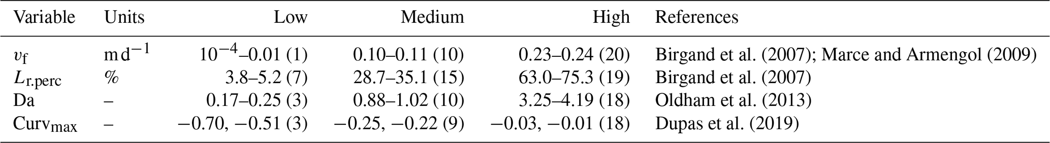
Table 1Network model parameter ranges for the Monte Carlo simulations.

a For vf, the selected range is an order of magnitude smaller than the one proposed by Marce et al. (2018) as we focus the analysis on the lower vf, where most of the bending happens (Sect. 3.3).
2.3 Exploring Curvmax with Monte Carlo simulations
Monte Carlo simulations are performed to explore how Curvmax evolves from a range of model input parameter combinations in a variety of catchments (Sect. 2.3.1 below). These simulations utilize the same ensemble of 11 107 unique parameter combinations in each of the individual study catchments with distinct observed discharge time series to account for the differences one parameter combination may have in each of the catchments. The unique parameter combinations are generated by Latin hypercube sampling from uniform parameter ranges that are set according to literature values (Table 1). Some physical constraints were also imposed such that the channel geometry parameters aw and ad must obey continuity principles ( and aw>ad, following Leopold and Maddock, 1953). Similar to Bertuzzo et al. (2017) the chosen parameter combination is kept constant in time and uniform in space for simplicity during one model run. The simulated variables are (i) Curvmax [–], deduced from simulated log (C)–log (Q) relationships when a minimum of 80 % of the C data are above the “detection limit” of 0.002 mg L−1 ; (ii) the network-wide percentage of load removed Lr.perc [%], which is calculated as the median of the ratio between the daily absolute removed load and the daily absolute incoming load in the river network; (iii) the median network travel time, TT [d]; (iv) the Damköhler number Da [–]; (v) the slope of the linear regression fit of the log (C)–log (Q) relationship at the catchment outlet, bout [–]; and (vi) the median concentration at the catchment outlet, Cout [mg L−1], and the median water velocity, v [m s−1]. While all outputs can be spatially and temporally explicit on a daily time step, Curvmax is examined at the catchment outlet, integrating both spatial and temporal aspects. The Monte Carlo results are subsequently subjected to a global sensitivity analysis with the PAWN method (Pianosi and Wagener; 2015) to elucidate influential model parameters. Furthermore a correlation analysis is conducted to explore how these influential parameters impact simulated Curvmax. Finally, a classification and regression tree algorithm (CART; Breiman et al., 1984) allowed us to visualize parameter interactions as detailed in Sect. 2.3.2 below.
2.3.1 Catchment selection
The river networks of 13 mesoscale catchments across Germany (areas between 21 and 1450 km2; Ebeling, 2020a; Table 2) are extracted together with the corresponding daily discharge data at the outlet (uninterrupted for ∼10 years between 1995 and 2010; Musolff, 2020) as inputs for the exploratory river network model. The selected catchments include three nested sub-catchments for the Selke as well as the Holtemme river system, both part of the Bode, a well-studied river system near the Harz mountains in central Germany (Fig. 1; Ehrhardt et al., 2019; Rode et al., 2016; Winter et al., 2021; Mueller et al., 2018). All catchments have distinct geophysical settings as stream order, median discharge and catchment shape (quantified with the Horton form factor; Horton, 1945; Table 2), which is needed to obtain a realistic range of simulated Curvmax using the explorative network model in the Monte Carlo mode. The selected catchments were delineated in ArcMap (ESRI, 2011) from a 100 m×100 m digital elevation model (DEM) (EEA, 2013; Ebeling et al., 2021). A flow direction, flow accumulation and valley slope grid in the same resolution were established. The channel threshold drainage area for the network delineation was set to 150 grid cells (1.5 km2), which agreed well with the observed river network, resulting in a tree-shaped river network with N grid cells or nodes.
Table 2Catchment properties summary: catchment area, median elevation, slope and topographical wetness index (TWI), maximum Strahler stream order, Horton form factor, drainage density, median discharge at the basin mouth over time (Q) with the corresponding runoff (area specific discharge) between brackets, and the coefficient of variation in the discharge in time (CV Q). The latter variable CV Q integrates the frequency of runoff events and the differences in recession constant (so the catchment's “flashiness” in response to rainfall) (Botter et al., 2013).
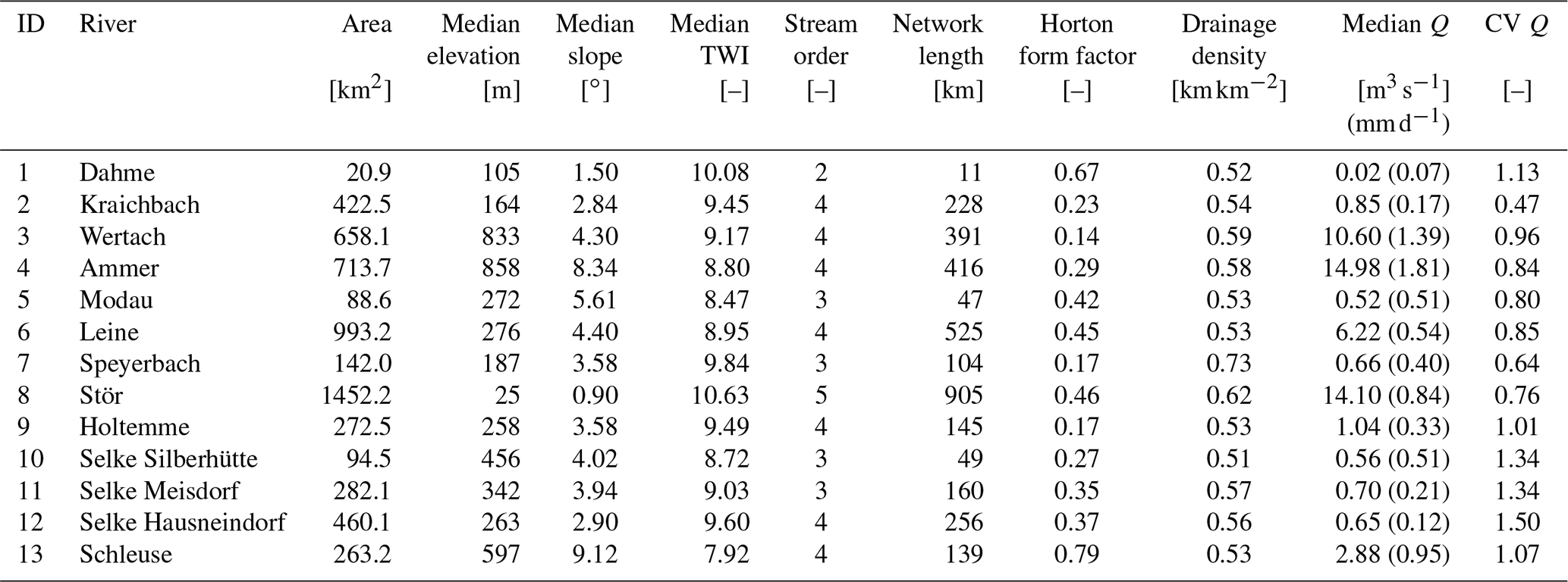
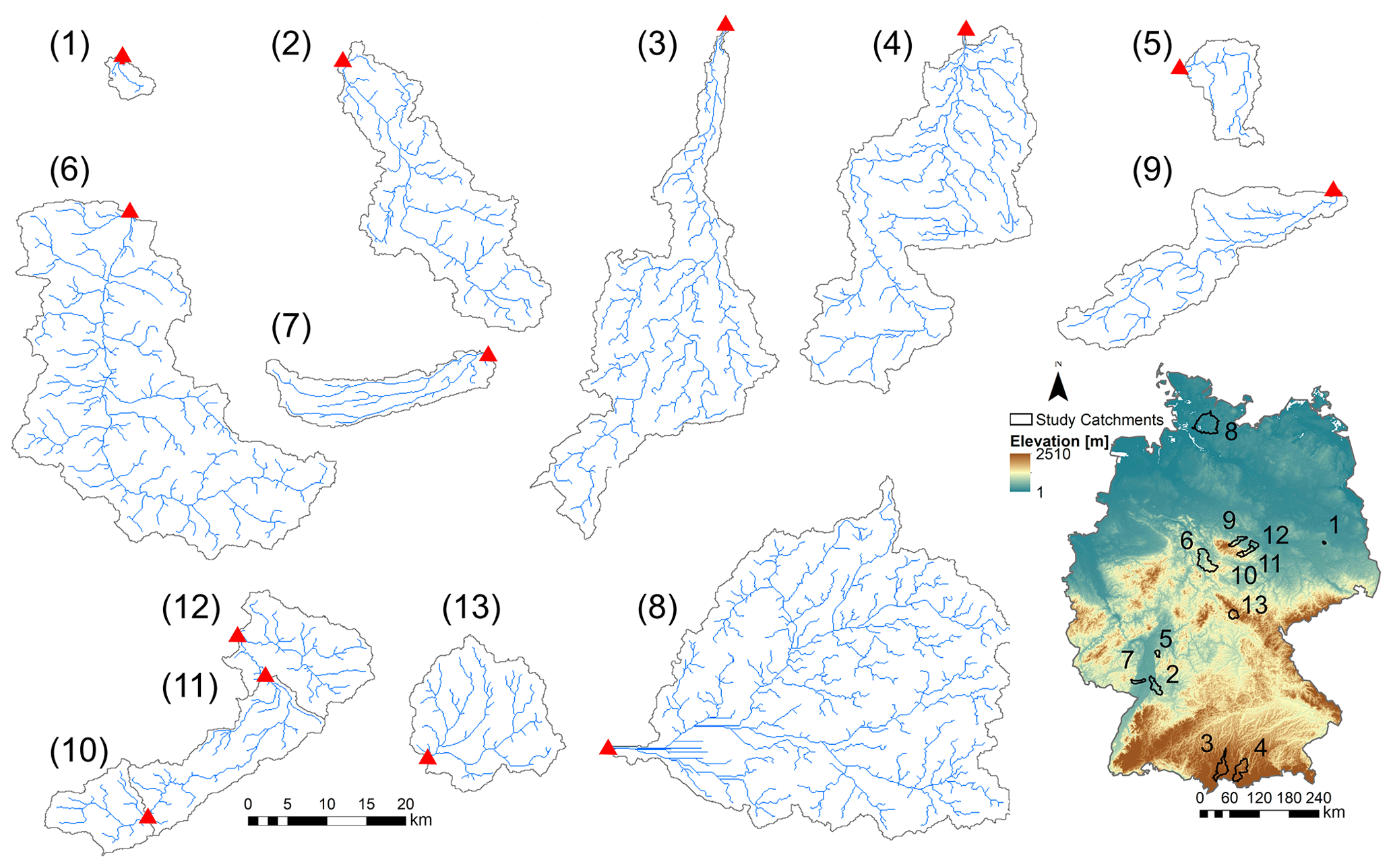
Figure 1Germany DEM with the location and outline (shape) of selected catchments, along with their drainage networks (in blue) and outlet location (red triangle). See Table 2 for catchment IDs and properties.
2.3.2 Model evaluation
To verify the network model's ability to reproduce realistic concentration time series and Curvmax, the observed monthly nitrate concentrations and the simulated time series were compared in 1 of the 13 selected catchments, the Selke catchment (at Meisdorf gauging station, 282 km2; Table 2; Winter et al., 2021), where extensive field campaigns and modeling studies have been conducted related to in-stream processes (Rode et al., 2016; Dupas et al., 2017; Yang et al., 2019, 2018). Note that such a model validation was performed only in the Selke Meisdorf catchment as the model aim is to explore how certain input parameter combinations may result in log (C)–log (Q) bending at the catchment outlet rather than to reproduce catchment-specific concentrations by performing parameter calibration. This explorative approach is comparable to Bertuzzo et al. (2017) and Helton et al. (2018), who applied a similar model in synthetic river networks but did not validate the model structure in a realistic setting. The Meisdorf catchment is a relatively homogeneous upstream part of the Selke, consisting of forest and cropland, and is characterized by constant export regimes (Winter et al., 2021). For an input parameter combination set to reasonable values for this catchment (Table C1; Rode et al., 2016), the land-to-stream inputs averaged 1.2 , which is similar to the 1.9 reported by Winter et al. (2021) for the Selke river (Meisdorf), and it is well within the general 0.001 to 100 range established by Mulholland et al. (2008). The simulated flow velocity had a spatiotemporal median value of 0.47 m s−1, which is also comparable with measured flow velocities (Risse-Buhl et al., 2017). Additionally, the Selke catchment was used to gain an insight into how the interplay of transport and uptake processes at every network grid cell can result in a curved C–Q pattern at the catchment outlet for one parameter combination, while in the other catchments the network model outputs were only considered at the catchment outlet for the entire range of input parameter combinations in the Monte Carlo approach. Finally, the simulated range of Curvmax, obtained from applying the network model in the 13 different catchments with >10 000 input parameters, was compared to a range of observed Curvmax computed from the C–Q relationships of 444 French catchments (Dupas et al., 2019; Sect. 2.1). Other Monte Carlo simulation outputs, such as ranges of Lr.perc and Da, were compared to literature values for validation purposes.
2.3.3 PAWN sensitivity analysis and correlation analysis
We performed a global sensitivity analysis (GSA) using the moment-independent PAWN method (Pianosi and Wagener, 2015). The method allowed for estimating the effect of the parameter inputs on the entire model output distribution and can be applied to rank the inputs and identify the uninfluential ones. The resulting PAWN sensitivity indices were estimated from generic input–output samples created with the numerical approximation strategy proposed by Pianosi and Wagener (2018). With this strategy, the range of variation in each input xi is partitioned into a number ni of equally probable “conditioning” intervals (Ii,k, ); i.e., each interval contains the same number of data points. Given a scalar model output y (here Curvmax), the PAWN method compares the output cumulative distribution function (CDF) (Fy(y)), computed by concurrently varying all the inputs, and the ni conditional CDFs for that input (). Each conditional CDF is obtained by varying all inputs within their entire range except for xi, whose values are contained within one of the ni conditioning intervals. The Kolmogorov–Smirnov statistic (KS) is then calculated as the maximum vertical distance between the conditional and unconditional CDFs, while the PAWN sensitivity index (Si) for input xi aggregates the results over all conditional CDFs through a summary statistic as presented in Eq. (7):
where .
In this study, we applied Eq. (7) using ni=10 conditioning intervals for each input parameter and used the maximum KS value, KSmax (ranging from 0 to 1), as a summary statistic, which is appropriate for screening non-influential input parameters. For a given parameter, the highest value of KSmax of 1 would indicate a direct dependence of the model output (in this case Curvmax) on that parameter, while a value of KSmax of 0 would mean that the parameter is completely non-influential. We estimated confidence intervals of the sensitivity indices using 15 000 bootstrap resamples and checked the robustness of the results. The PAWN analysis was carried out using the Python version of the SAFE toolbox for global sensitivity analysis (Pianosi et al., 2015).
To explore the direction of change in the C–Q bending at the catchment outlet resulting from variations in the model parameters and the catchment in-stream uptake, a Spearman rank correlation analysis was performed including all the simulated catchment responses and parameter combinations. These correlations were visualized in a correlation matrix using the “corrplot” package in R (Wei and Simko, 2017).
2.3.4 Identify parameter and model output interactions with classification tree
Finally, we aim to determine if, within this modeling framework, C–Q bending at the catchment outlet (specifically Curvmax) informs about the network-wide in-stream uptake. Thereto, a recursive modeling approach is proposed, using the classification and regression trees algorithm (CART; Breiman et al., 1984), which allows for the identification of non-linear synergistic interactions among model parameters and output variables. This non-parametric method segregates classes for a response variable by progressively splitting selected predictor variables in a binary way. The resulting decision tree is intuitive to interpret and can facilitate the fast characterization of river networks. The response variables include the effective catchment-wide removal efficiency Lr, the Damköhler number Da and the uptake velocity vf, while the predictors are Curvmax, the median network velocity v and all of the model input parameters except for vf (Table 1). For each response variable, three classes are defined representing low, intermediate and high ranges found in the literature (Table 3) that each contain 5 % of the simulation outputs (obtained by distributing the non-missing model simulations over 20 percentiles). The overall CART accuracy for each response variable is assessed by attributing 80 % of the simulation outputs in the low, intermediate and high classes to a training sample and assigning the remaining 20 % to a test sample. The training sample is then used to construct the classification tree, while the test sample is needed to assess the prediction accuracy and calculate the performance statistics for each class. The CART analysis was performed using the “caret” package in R with the Gini impurity measure as a splitting criterion (Kuhn, 2020).
Table 3Classes containing low, medium and high values for response variables vf (uptake velocity), Lr.perc (percentage of load removed) and Da (Damköhler number) are used for the CART training and testing samples. Similar classes are obtained for model output Curvmax. These classes stem from distributing the non-missing simulation data over 20 percentiles and selecting the percentiles corresponding to low, medium and high literature values, with the respective percentile number (1–20) indicated in brackets. This was done to ensure that for one variable, each class contains the same number of simulation data points. The training sample for constructing the CART model was then allocated 80 % of this data and the test sample 20 %.
3.1 Empirical Curvmax
The estimated Curvmax for the French observed log (C)–log (Q) data (Dupas et al., 2019) ranges between −5.25 and 3.88 (median is −0.23; Fig. B4), and 77 % of the stations are characterized by Curvmax≤0 or a linear or concave shape (similar to Moatar et al., 2017). The time series subsamples for each station generally had a small Curvmax variability (interquartile range, IQR, for a given station below 1) for 93 % of the stations, with some exceptions demonstrating a larger IQR up to 8. This indicates that Curvmax quantification for most low-frequency C–Q time series is robust. The Spearman rank correlation (ρ=0.53, ) between the absolute observed Curvmax and IQR for each station is significant and positive, implying that C–Q relationships with a higher absolute Curvmax have a higher uncertainty when quantifying the C–Q bending. However, Curvmax variability (IQR) in the subsamples for each station has no significant correlation with the number of data points available for one station. This implies that Curvmax tends to be temporally robust when the C–Q data obey the four criteria in Sect. 2.1 so that the length of the low-frequency time series does not impact the estimated Curvmax. Overall, the proposed Curvmax metric is suitable to quantify bending in multi-annual, temporally stable log (C)–log (Q) relationships.
3.2 Model evaluation in the Selke river (Meisdorf)
To evaluate the network model performance in a realistic setting, we implemented the model with a fixed parameter combination (Table C1) in the Selke catchment and aimed to capture C–Q dynamics at the basin outlet. The simulated concentration time series (simulated C with uptake) for the Meisdorf station in Fig. 2a shows a seasonal pattern that follows the observation concentration data reasonably well (Nash–Sutcliffe efficiency, NSE=0.50; percent bias, This seasonality is also reflected in simulated daily percentage of load removed (the ratio between the daily total removed load and the daily total incoming load in the river network) and ranges from almost 0 % to 3.4 % in this case, with the median Lr.perc value equal to 0.41 %. The highest removal efficiencies are simulated in fall and summer and coincide with low simulated concentrations at the catchment outlet. The conservative concentration (simulated C no uptake) is stable around 3 mg L−1. The observed nitrate concentrations generally show an enrichment export pattern in the log (C)–log (Q) space (bout=0.40, R2=0.56) and a Curvmax of −0.35, which agrees well with the simulated Curvmax of −0.28 (Fig. 2b) and deviates significantly from the conservative scenario of simulated C without uptake (b=0.014; Table C1). The observed low nitrate concentrations coincide with low discharges in fall and summer, while high concentrations occur mainly in winter, when discharges are higher.
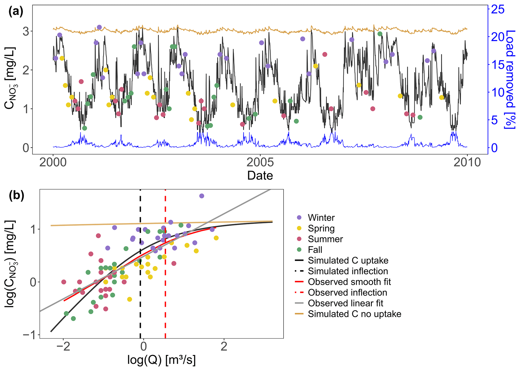
Figure 2(a) Simulated and observed concentrations at the Selke Meisdorf gauging station for a 10-year simulation period (2000–2010; NSE=0.50). One data point (C∼5 mg L−1) is not shown here. The simulated median percentage of load removed in the stream network (blue line) is given during the same time period as well as the simulated C with no uptake (vf=0). (b) The observed concentrations and Q are log-transformed and plotted together with the simulated C–Q data for 2000–2010. A smoothed spline is fitted to the observed and simulated C–Q data (described as observed smooth fit and simulated C, respectively, in the legend), and Curvmax values of −0.35 and −0.28 are calculated at the respective discharges of 1.72 and 0.92 m3 s−1, indicating the smoothed spline inflection points.
Within the Selke Meisdorf river network the simulated Curvmax is largely contained within −1.12 to −0.29 (10th and 90th quantiles, respectively) for the given parameter combination (Table C1, Fig. 3). Low Curvmax () is found exclusively at grid cells with a low total drainage area (Ai<9 km2), and Curvmax stabilizes at higher values with increasing drainage areas (inset Fig. 3, Fig. S3 in the Supplement). The incoming (Lin.ls and Lin.up; Eq. 3), removed (Lr; Eq. 5) and outgoing absolute load (Li; Eq. 4 with L=CQ) as a function of Q in the log–log space are shown in Fig. 3 for three selected grid cells on the main river stem with low (C), intermediate (B) and high (A) drainage areas. The corresponding log (C)–log (Q) relationship for the outgoing load (Li) at the outlet (A) is presented in Fig. 2b for simulated and observed values. Note that Curvmax is calculated from log (C)–log (Q) relationships rather than log (L)–log (Q). The loads in grid cell A, B and C generally increase with discharge, while the load removal efficiency decreases with discharge. The highest removal efficiencies are found in the headwater grid cell C (39 % for low discharge), followed by mid-stream grid cell B (3 % for low discharge) and the outlet A (0.5 % for low discharge). The total absolute load removed (Lr, sum per year per grid cell) is largest for first-order grid cells (average 24.1 kg N yr−1) that represent 55 % of the river network, followed by second- and third-order grid cells (averaging both around 20 kg N yr−1) that represent 20 % and 25 % of the network (inset Fig. 3). Finally, the total yearly incoming load (Lin.ls+Lin.up, sum per year per grid cell) increases with stream order from 1329 kg N yr−1 on average in a first-order grid cell to 5128 and 42 124 kg N yr−1 in second-order and third-order river cells.
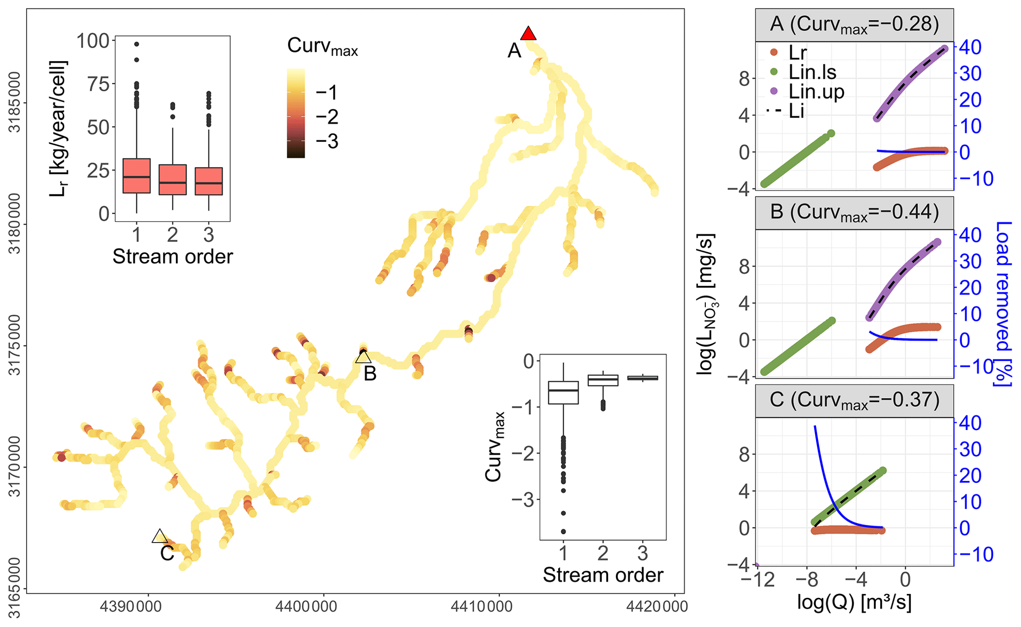
Figure 3Spatial distribution of simulated Curvmax in the Selke river network (Meisdorf) for a selected parameter set (see Table C1). Three representative grid cells covering low (A), intermediate (B) and high (C) total drainage areas show the incoming land-to-stream load as Lin.ls (Eq. 3), the incoming load from upstream as Lin.up (Eq. 3), the absolute removed load as Lr (Eq. 5) and the outgoing load as Li (Eq. 4) in the log (L)–log (Q) space. The load removed as a percentage of the incoming load is presented on the secondary axis. Note that the corresponding Curvmax values for these grid cells are calculated from the log (C)–log (Q) relationships rather than log (L)–log (Q). The insets show the distribution of Curvmax and Lr for each grid cell within a certain stream order. In Fig. 2a the observed and simulated concentrations are compared at point A.
With uniform, constant parameters the network model does not account for a spatiotemporal parameter variability. Nevertheless, it successfully (see NSE and pbias) reproduces the seasonality of the observed concentrations over the 2000–2010 period for the Selke Meisdorf catchment (Fig. 2a). For comparison, Yang et al. (2018) found a similar performance (NSE=0.47, %) when applying a fully distributed model with 16 calibrated parameters in this catchment between 1997 and 2009. The uptake velocity vf for our simulation was set to 0.098 m d−1 to closely match the observed (assimilatory) uptake range of 0.009 to 0.103 m d−1 for the Selke Meisdorf river network (Rode et al., 2016); the median annual percentage of load removed equals 4.7 %, which is within a comparable range reported in prior studies (Rode et al., 2016, and Yang et al., 2018, found annual means of 4.8 % and 7.6 %, respectively). Note that the annual percentage of load removed accounts for load taken up throughout the entire river network, which may be higher in the headwaters (15 t) than in downstream locations (7 and 5 t for second- and third-order stream sections; inset Fig. 3). Yang et al. (2018) reported very high uptake efficiencies (up to 75 %) for summer seasons that were caused by low concentrations (0.21 mg N L−1) and load (L=CQ), which are not represented in our model simulation (the lowest simulated concentration equaled 0.4 mg N L−1). Additionally, due to the parsimonious structure of the proposed model, we did not account for the temporally changing effects of environmental factors like temperature and light availability that might (seasonally) influence uptake efficiencies in the river network (Kadlec and Reddy, 2001). Nevertheless, these high uptake efficiencies under low flows in summer are not a main contributor to the annual percentage of load removed that is dominated by high flows, generally recorded during winter. Thus for the Monte Carlo simulations we calculated Lr.perc as the median of the daily percentage of load removed rather than the total removal efficiency for the entire simulated time period to better represent an effective long-term network-wide removal capacity.
The interplay of incoming, removed and outgoing load at each network grid cell shapes the log (L) and log (C)–log (Q) relationships and consequently Curvmax at the catchment outlet (Fig. 3). Land-to-stream loading (Lin.ls) that varies linearly with direct incoming discharge at a given grid cell in the log space (Eq. 3 with L=CQ; Curvmax=0) can lead to a bent outgoing log (C)–log (Q) relationship where concentration or load (Li) varies non-linearly with discharge (Curvmax≠0). The onset of a bent log (C)–log (Q) pattern () is illustrated in the headwater grid cell C in Fig. 3, where Lin.ls is the only incoming load (upstream incoming load, Lin.up, equals 0 in this case). The absolute removed load in a grid cell is higher under increasing Q, while the percentage of load removed is lower, which explains observed C–Q patterns with higher log (C)–log (Q) slopes for low flows than for high flows (Moatar et al., 2017; Wollheim et al., 2008, 2017; Doyle, 2005; Basu et al., 2011). This decreased load removal efficiency in the downstream direction (spatial scale) or during events (temporal scale) can arise because stream morphology characteristics such as depth and water velocity that correlate with varying discharge constitute higher surface-to-volume ratios at low flows (generally in the headwaters) than at higher flows (at the outlet) (Peterson et al., 2001; Hensley et al., 2014). The uptake and land-to-stream loading at the downstream grid cells (B and A in Fig. 3) have a decreasing local impact on the outgoing load due to the large upstream load contributions that increase in the downstream direction (see explicit scaling relationship for input flux in Bertuzzo et al., 2017). This is also explained by Wollheim et al. (2018), who suggest that the river network saturates as supply exceeds biological “demand”, causing the log (C)–log (Q) relationship to approach the slope of the loading function (presented as the simulated C without uptake in Fig. 2b). Dupas et al. (2017) on the other hand show how uptake effects are decreasingly visible in C–Q observations downstream, and concentrations largely matched those estimated by a conservative mixing model. The saturation effect with the accumulation of large load is reflected in the Curvmax converging to a constant value when moving from upstream to downstream or from a lower-order to a higher-order river reach (Figs. 3 and S3). This also corroborates the recent findings of Abbott et al. (2018), who found that the temporal variability (here reflected in the C–Q relationship) in nutrients is preserved moving downstream in a river network. Overall the Selke example shows that the network model can realistically reproduce the bending of observed C–Q relationships that evolve from the decreasing removal efficiency at higher discharges.
3.3 Monte Carlo simulation results
The overview of the model outputs for each of the 13 study catchments in Table 4 shows that catchments 1, 5 and 11 display the lowest 10th quantile Curvmax values of −1.61, −1.40 and −1.24 (more bending), while the catchments 4 and 6 registered higher (less bending) and less variable Curvmax (10th quantiles at −0.31 and −0.35) (Fig. B5). Catchments 3, 4 and 8 are characterized by high runoff and Q (Table 2) at the catchment outlet and demonstrate low percentages of load removed, Lr.perc (90th quantile at 29.8 %, 32.1 % and 19.3 %, respectively). The highest Lr.perc values are found in catchments 1 and 10 (98.4 % and 95.1 % for the respective 90th quantiles). The regression slope of the log (C)–log (Q) relationship at the basin outlet, bout, is positively skewed for all the catchments (most positive slopes found in catchment 5), while the slope b of the land-to stream loading function had no positive or negative preference (Table 1, Eq. 3). The distribution of the concentrations at the catchment outlet, Cout, are generally similar across all catchments (10th and 90th percentiles within 0 to 6.2 mg L−1) and are significantly less variable than the land-to-stream incoming concentration (parameter Cmean) that varied from 10−4 to 20 mg L−1 across all the simulations (Table 1). The highest Cout values are found in catchment 8, the largest catchment. The median water velocity v (Eq. 2c) is between 0.01 and 0.5 m s−1 for the 10th and 90th quantiles of all the study catchments, and the largest v is simulated for catchments 3 and 4, which also have the highest discharge. The median river network travel time, TT, for all simulations and catchments ranges from 0.1 to 4 d between their respective 10th and 90th quantiles and remarkably has no clear relationship with catchment properties such as the total river network length (Table 2). Finally, the Damköhler number, Da (Eq. 6), is variable around 1 with the highest values, indicating reaction-driven conditions, found for catchments 2 and 12 (respective ranges from 0.6 to 10.3 and 0.7 to 10.8 for the 10th and 90th quantiles). The lowest Da values are found for catchments 4 and 10 (90th quantile <2), implying more transport-driven conditions.
Table 4The 10th, 50th and 90th quantiles of model outputs Curvmax, percentage of load removed, (Lr.perc) Damköhler number (Da), regression slope of the log (C)–log (Q) relationship at the basin outlet (bout), the median concentration at the basin outlet (Cout), the median water velocity (v) and median river network travel times (TT) for each of the 13 German catchments.

The Monte Carlo output in Table 4 shows reasonable values for the different variables, taking into account that the goal of this modeling exercise was not to reproduce catchment-specific conditions but rather to explore how uptake influences C–Q bending for a range of parameter combinations that represent a spectrum of possible catchment conditions. The simulated Curvmax values for all 13 German study catchments and parameter combinations (80 % of the values between −0.70 and −0.012; Table 4 and Fig. B5) are comparable with the range of Curvmax from log (C)–log (Q) relationships in the French catchments (80 % of the values between −0.41 and −0.067; Fig. B4) (Dupas et al., 2019). Simulated Curvmax is always smaller than or equal to zero as explained in Sect. 2.2.2. For the model output Lr.perc, a wide range of uptake efficiencies were captured from almost 0 % to near to 100 % for some simulations and a median value of 14.4 % across simulations. This simulated range exceeds the proposed range by Birgand et al. (2007) of 10 % to 70 % of N removal for agricultural drainage networks at annual timescales. High removal percentages (median over the simulated time period of daily percentage of load removed in the network exceeding 95 %) are registered for 3.4 % of all simulations, while very limited load removal (Lr.perc<5 %) occurred for 32.1 % of all the simulations. Other simulation outputs such as the effective velocity v surprisingly rendered similar distributions across the catchments (Table 4) given that the median Q varied for almost 3 orders of magnitude at the basin outlet (Table 2). Their specific discharges (Sect. 2.2.1) however are similar, and by taking the spatiotemporal median v as an effective catchment value for each simulation the (more numerous) headwater grid cells were better represented than the grid cells close to the basin outlet. A similar effect is found for the range of the effective travel time TT. Generally these similar v and TT distributions from model simulations between catchments align with the notion of Langbein and Leopold (1964) that drainage networks evolve naturally to transport water (and sediment) most efficiently such that an equilibrium between channel form and water and sediment load is imposed (Leopold and Maddock, 1953). Also Damköhler numbers Da exhibited realistic ranges, mostly distributed around 1 (Fig. S3; Oldham et al., 2013; Ocampo et al., 2006), with 36.5 % of the simulations <0.8 % and 50.8 % > 1.2, indicating that more simulations are reaction-driven than transport driven. Finally, other variables such as the range of the modeled river widths are found to be reasonable to a large degree (Fig. S4 in the Supplement).
As for the simulations, the same >10 000 parameter input sets are applied in each catchment, differences between the catchments result from the different network structures and hydrological regimes that control transport and uptake processes for each parameter input set in each catchment. From Tables 4 and 2 it is clear that differences in model outputs (i.e., Curvmax, Lr.perc and Da) between the catchments cannot be attributed to a single catchment property such as total network length or basin area. For example Curvmax has the highest variability between simulations in the catchment 1, the smallest catchment, compared to the other catchments, which could be attributed to the variability in local loading and uptake patterns in the network (driven by Q) that are still visible at the catchment outlet. Following the simulated Selke Meisdorf example in Sect. 3.1 (Figs. 3 and S3), we show that Curvmax tends to converge to a constant value with increasing drainage areas (similar to Abbott et al., 2018, for nutrient concentrations; Dupas et al., 2017, for nutrient uptake; and Bertuzzo et al., 2017, for DOC removal). Drainage area is however not the only catchment property influencing Curvmax at the outlet. For example, catchment 6 is the second-largest catchment (Table 2) and has the least bent (and least variable) log (C)–log (Q) relationships. The network structure could possibly play a role here as the largest catchment, catchment 8, has some large tributaries near the basin outlet (Fig. 1), which could bypass removal and transport high load during events, introducing a more variable Curvmax (Mineau et al., 2015; Helton et al., 2018). The percentage of load removed, Lr.perc, is notably lower for catchments with high runoff or Q – like 3, 4 and 8 (Table 4) – which corresponds with findings in Sect. 3.1 that uptake efficiency decreases with increasing Q because of increasing loads to the system (Wollheim et al., 2018; Mulholland et al., 2008) and that increasing Q results in less efficient uptake within the reactive surface area (Peterson et al., 2001; Hensley et al., 2014). The high Lr.perc in small catchments 1 and 10 could then be attributed to their low Q; however why the small catchment 5 does not have similar uptake performance is not evident. Generally the model output variability between the catchments (as a result of different network and discharge properties) is minor compared to the output variability within the catchments (due to the effect of the chosen input parameter set).
3.4 Curvmax sensitivity analysis and model parameter correlation
The PAWN sensitivity index KSmax in Fig. 4 and Table C2 shows that across all catchments Curvmax is most sensitive to the exponents in the width–Q relation aw (KSmax=0.62) and depth–Q relation ad (KSmax=0.51). Here, there is little variability between the catchments (KSmax has a low coefficient of variation, CV, of 0.06 and 0.22, respectively). Overall, the slope of the linear loading function, b, is least important in shaping Curvmax (KSmax=0.14). Nevertheless, a high variability in KSmax is observed (CV=0.76) that is caused by larger sensitivities for catchments 1 and 12 (KSmax near 0.45). Curvmax is equally sensitive to vf and Cmean (KSmax 0.18 and 0.19), but vf exhibits higher variability in KSmax than Cmean (CV of 0.59 and 0.47). Furthermore, over all the catchments Curvmax is sensitive to the median velocity v and the Damköhler number Da (KSmax equals 0.64 and 0.31, respectively; CV of 0.26 and 0.38). When considering the catchments individually, basin 1, with the smallest discharge, has the highest median KSmax (0.59) across all input parameters, while catchment 4, which has the highest discharge, exhibits the lowest median KSmax (0.13). Additionally, Curvmax is very sensitive to the velocity v in catchment 1 (KSmax=0.95), while it is least sensitive to v in catchment 4. Nevertheless, the other catchments show no clear order in Curvmax sensitivity according to catchment properties such as Q. For example in nested catchments 10, 11 and 12 (Fig. 1), the largest catchment, catchment 12, has the highest KSmax (0.50) and lowest CV (0.26) over all the input parameters, indicating that here Curvmax is more sensitive to the input parameters than in the smaller sub-catchments 10 and 11.
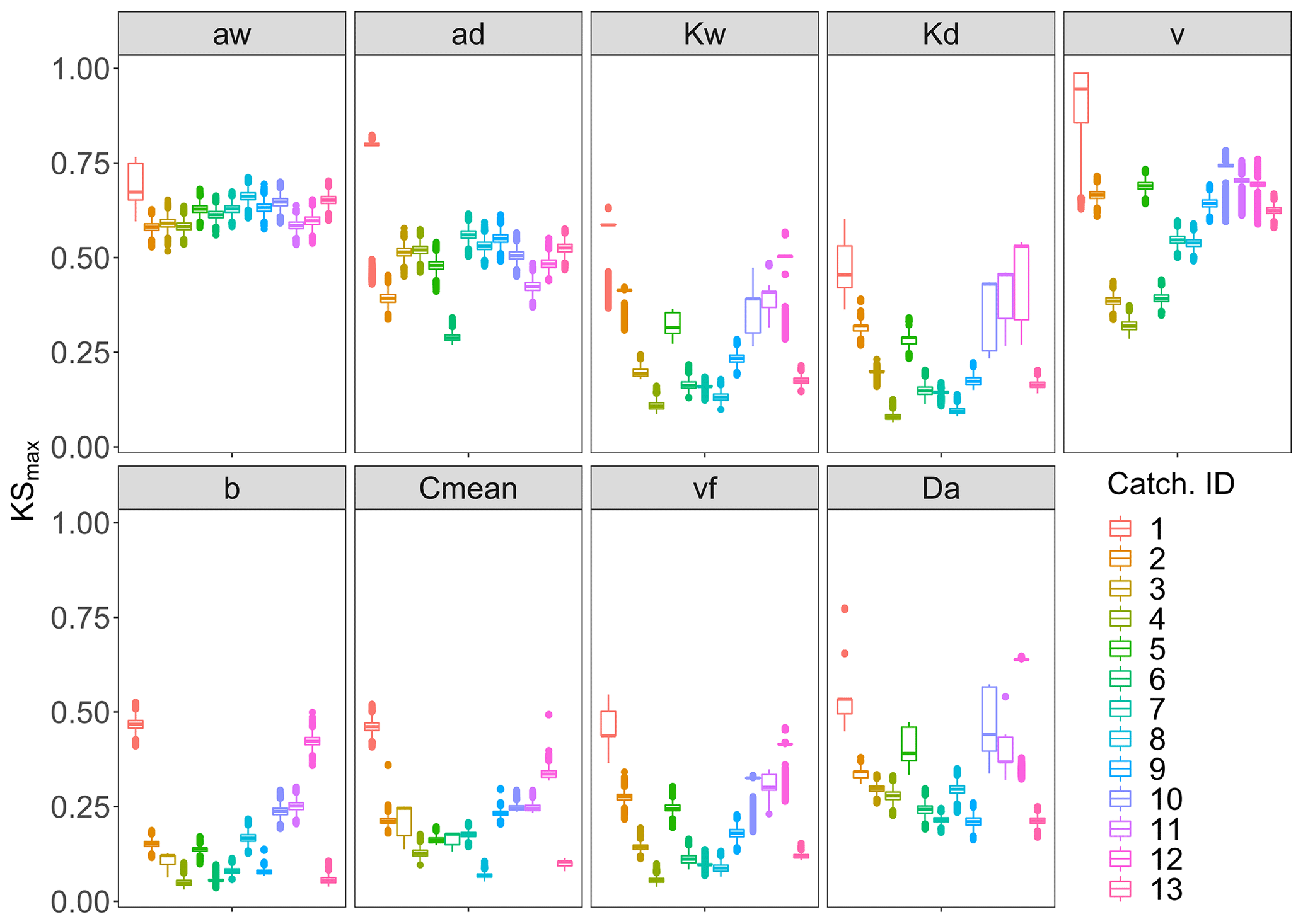
Figure 4The KSmax sensitivity index for each of the model input parameters and each of the 13 simulated catchments. The input parameters related to the channel geometry (ad, aw, Kd and Kw), land-to-stream loading (b and Cmean) and biogeochemistry (vf) are shown together with two variables derived from some of the input parameters: the median velocity v and the Damköhler number Da. Each boxplot displays 15 000 bootstrapped estimates of KSmax for each of the 13 simulated catchments.
In a next step the estimated Curvmax across all simulations is correlated to the model input parameters as well as to output variables like the percentage of load removed (Lr.perc) the log (C)–log (Q) slope at the catchment outlet (bout), the median concentration at the basin outlet (Cout) and the uptake constant (k) to identify the strength and direction of their relationship. The resulting Spearman correlation matrix (Fig. 5) reflects the PAWN sensitivity findings, with the highest Curvmax correlation found with parameters aw (ρ=0.68) and ad (ρ=0.56) and input variable v (ρ=0.57). Curvmax is independent of vf () but shows a negative correlation with Lr.perc (), suggesting that lower Curvmax (more bending) can be related to a higher Lr.perc. Furthermore, Curvmax is negatively correlated to the log (C)–log (Q) regression slope at the catchment outlet bout () such that higher bending coincides with more positive bout. The variable v is additionally strongly negatively correlated with Lr.perc (), so a high percentage of load removed occurs at low velocities. Da on the other hand is positively correlated to Lr.perc (ρ=0.58), which indicates that higher Da values are occurring together with higher load removed. Da thereby seems to be controlled more tightly by variation in k−1 () than by TT (ρ=0.48). Finally Cout is negatively correlated with Lr.perc () and Da ().
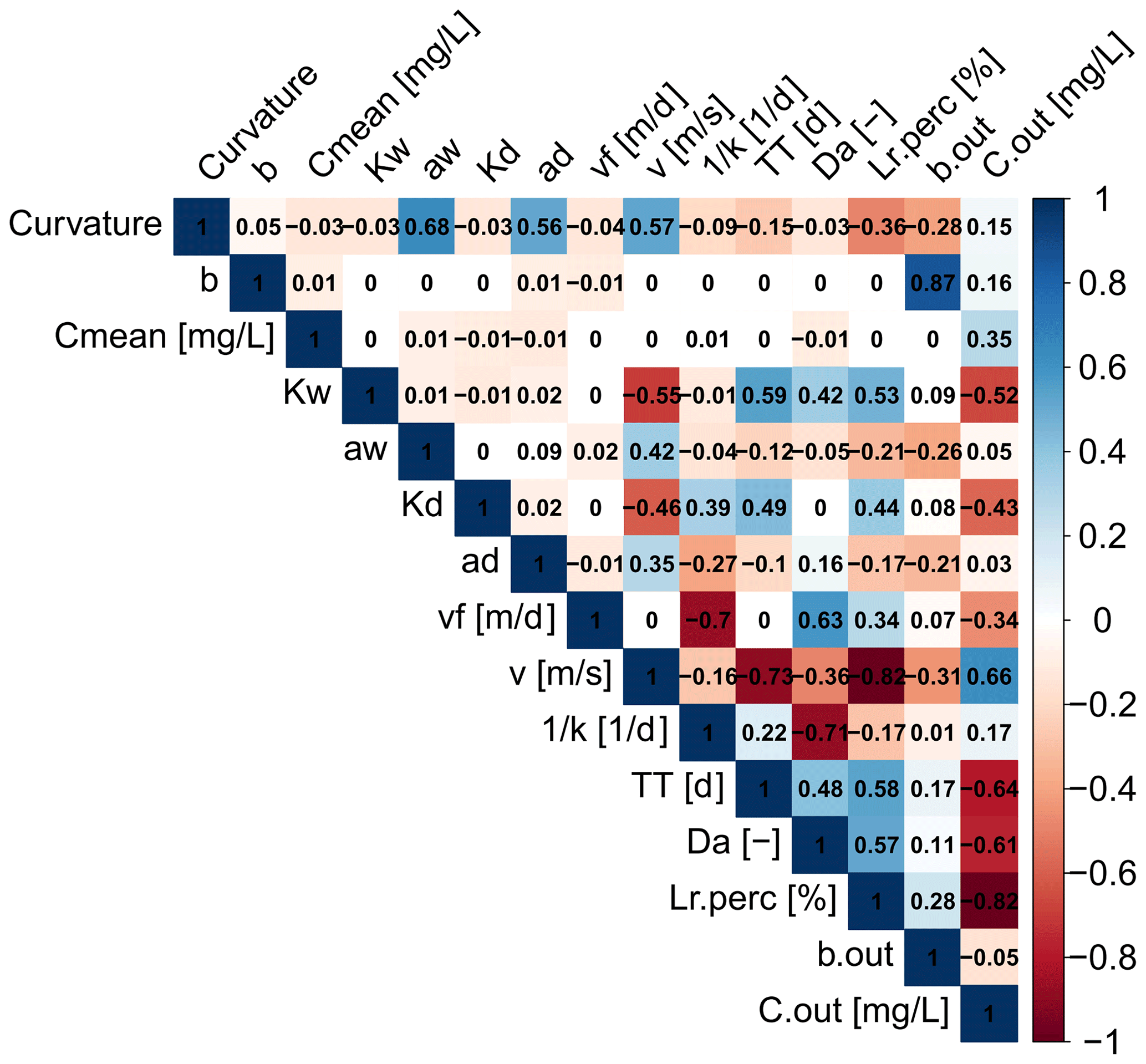
Figure 5Correlation matrix for the model parameter inputs: channel depth and width exponents (ad, aw) and coefficients (Kd, Kw); slope of the land-to-stream loading (b); concentration of the land-to-stream load (Cmean); uptake velocity (vf); and the outputs bending of the log (C)–log (Q) relationship at the catchment outlet (Curvmax), effective stream velocity (v), first-order uptake constant (k), travel time (TT), Damköhler number (Da), daily percentage of load removed (Lr.perc), and slope of the log (C)–log (Q) relationship and median concentration at the outlet (bout and Cout). The Spearman rank correlation coefficients (ρ) are given for each combination.
The PAWN and correlation analysis results suggest that the input parameters dictating the channel morphology, aw and ad (Sect. 2.3), are controlling factors for the magnitude of the bending in log (C)–log (Q) relationships at the catchment outlet. More specifically parameters aw and ad influence the response of the wetted perimeter (Pi; Eq. A2) in a given reach in the network and drive the reactive surface area (Pi⋅li) with changes in discharge (Eq. 2a and b, Figs. 5 and B3). The absolute load removed Lr,i (Eq. 5) can be written with the width and depth exponents aw and ad explicitly (Eq. A3) so that . When the denominator is large (small aw and ad) the effect of low and high Q's on the local absolute removed load increases and can lead to a lower Curvmax (more bending; Sect. 3.1, Fig. B6). Network-based modeling studies often set the width exponent aw to a value of 0.5 that was found to be representative of rivers globally (Bertuzzo et al., 2017; Rode et al., 2016; Wollheim et al., 2018). This a priori fixed aw may, however, strongly affect the simulated C–Q dynamics at the basin outlet as is demonstrated here. Curvmax finally shows the lowest sensitivity to the loading parameters b and Cmean that influence the incoming load to a grid cell (Eq. 3) and thus impact the local absolute load removed Lr,i (Eq. 5) rather than the percentage of removed load Lr.perc. This indicates that the contribution of local incoming load in the downstream direction has a limited impact on the log (C)–log (Q) bending at the catchment outlet. For example in the Selke Meisdorf catchment, the locally contributing Q's are generally smaller (or equal for the headwaters) than the total Q in a given reach so that the influence of the loading parameters b and Cmean on the total load decreases in downstream reaches (Sect. 3.1, Fig. 3).
Although Curvmax only has an intermediate sensitivity to the uptake velocity vf, and they do not correlate well, vf is an important “boundary condition” for log (C)–log (Q) bending at the catchment outlet. No biological demand (low vf) would mean that none of the incoming load would be removed from the river network. The outlet signal would in this case be solely driven by the discharge-controlled transport processes, and no bending would be observed (Curvmax=0). Although increasing vf does correlate with decreasing concentrations () and increasing load removed (ρ=0.34), it does not always lead to more bending, as illustrated in Fig. B6 for the Selke example. Because vf is defined as a constant within one simulation that is independent of the local nutrient concentration (Sect. 2.2.2), the percentage of load removed in the network is mainly controlled by the varying hydrological conditions here, represented by the effective network-wide velocity v (Lr.perc and v, ). This confirms that discharge and channel morphology are among the most important predictors of removal (Alexander et al., 2000; Seitzinger et al., 2002; Wollheim et al., 2006). The role of v was further examined in the context of restored and channelized streams (Kunz et al., 2017) and agrees with our findings that decreased v influences N cycling (Peterson et al., 2001).
The PAWN and correlation analysis results show that Curvmax is sensitive to the Damköhler number Da (KSmax=0.31; Fig. 4, Table C2), which has a high positive correlation with the percentage of load removed Lr.perc (ρ=0.58; Fig. 5). This indicates that high Da occurs concurrently with more efficient removal and is in line with others (Ocampo et al., 2006) who found sometimes almost 100 % removal in the riparian zones of an agricultural catchment with Da exceeding 2. The transport timescale TT that makes up Da (ρ=0.48; Fig. 5) together with the inverse of the first-order uptake constant k−1 (; Eq. 6) is examined for classes of low, median and high Da (defined in Table 3) in Fig. 6a to disentangle which values of k−1 and TT occur together and can constitute a certain Da range (each class contains 5 % of all simulations). It is shown here that low Da values are driven by both low TT and high, variable k−1, implying a transport-driven system with limited removal (median Lr.perc equals 2.4 % in Fig. 6a for low Da). High Da values, contrarily, have high TT and low k−1, fostering intermediate uptake percentages (median Lr.perc=27.1 %). Although also vf clearly differentiates for classes of low, medium and high Da in Fig. 6a, the corresponding Curvmax values are similar in their range and mean. Nevertheless, this does not mean that Da is not influencing Curvmax at the basin outlet as there could be interactions with other inputs that are not captured here (which is supported by the PAWN findings, where Da appears to be influential).
From the Curvmax perspective (Fig. 6b) we identify model output ranges of Lr.perc, Da and input variable vf that constitute low, median and high Curvmax classes (Table 3). High Curvmax (less bending, ) is thereby linked to low Lr.perc (median 4.8 %), while low Curvmax (more bending, ) is connected to higher and more variable Lr.perc (median 33.6 %), generally indicating that more bent systems are more efficient in terms of removal and vice versa. To explore some cases when this latter statement might not be true, we examine the input parameter ranges where more bent simulations (, 13.1 % of all simulations) occur concurrently with low percentage of removal (Lr.perc<5.2 %, 0.9 % of all simulations) on the one hand and high percentage of removal (Lr.perc>63.0 %, 4.9 % of all simulations) on the other hand in Fig. B7a. Here, it is seen that high-bending, low-uptake cases mainly occur for simulations with a high effective velocity v (driven by lower values for the channel shape parameters Kw, Kd, aw and ad). Low aw and ad are correlated with more bending (low Curvmax), and Curvmax is most sensitive to these parameters. However, low aw and ad do not lead to a more efficient uptake if the other channel shape parameters Kw and Kd cause relatively high velocities (median v>0.1 m s−1) throughout the network. The latter case is shown to be true for a minor percentage of all simulations (0.9 %) and explains why low Curvmax (more bending) can be connected to a wider range of Lr.perc. Figure B7b shows that concurrent simulations of less bending () and high removal (Lr.perc>63.0 %) are even rarer (0.1 % of all simulations) compared to concurrent less bending () and low removal (Lr.perc>5.2 %; 7.4 % of all simulations). Deviations from the expected high Curvmax–low Lr.perc pattern are also here driven by (very low) v. In the latter case however, aw and ad are generally high (leading to high Curvmax), and the different v values stem from coefficients Kw and Kd, which are higher in high-removal simulations. Finally, Fig. 6d illustrates that low, medium and high uptake velocities vf lead to distinct Da and Lr.perc but do not show up in the bent signal at the catchment outlet.
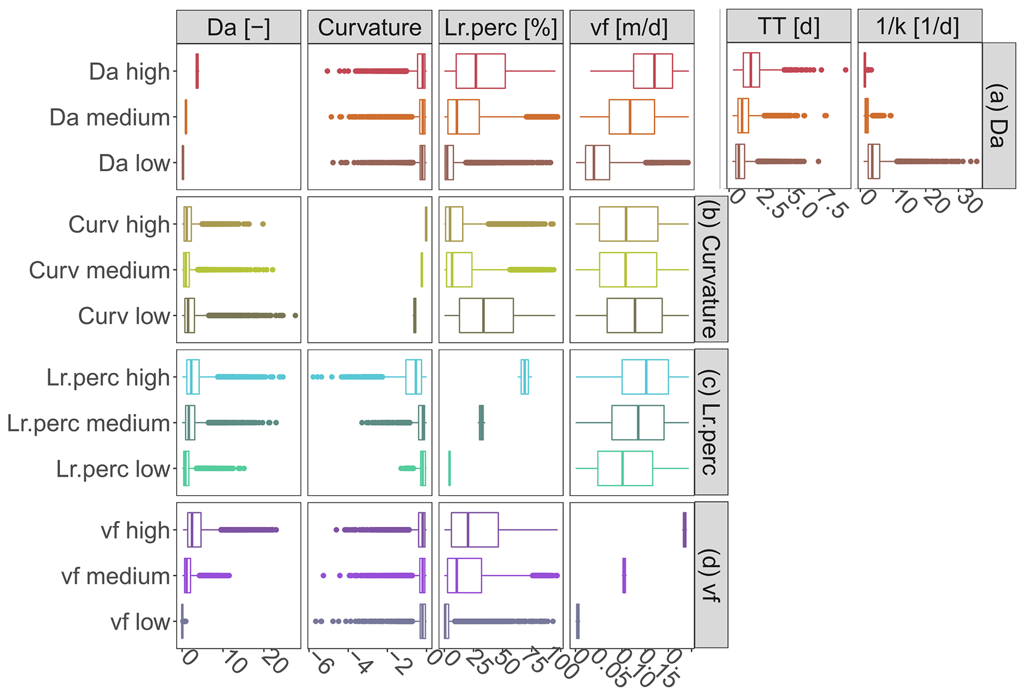
Figure 6The corresponding simulated ranges for high, median and low values (Table 3) of the main simulation outputs: (a) Damköhler number Da, (b) Curvmax, (c) percentage of load removed Lr.perc and (d) uptake velocity vf are shown for the same variables (in the columns). The median travel time, TT, and the inverse of the first-order uptake constant, k−1, are given additionally for low, medium and high Da.
3.5 Predicting in-stream processing with Curvmax
To determine if observed C–Q bending at the catchment outlet (here Curvmax) can be utilized to quantify in-stream uptake in the upstream river network and to visualize model parameter interactions, a classification tree was established for low, medium and high values (Table 3, Fig. 6) of the response variables Lr.perc, Da and vf (Fig. 7). The prediction accuracy metrics in Table C3 and the probability histograms in Fig. 7 show that Lr.perc can be predicted relatively well (overall accuracy of 0.66) compared to the other response variables Da (accuracy 0.51) and vf (accuracy 0.40). The fitted CART models all perform significantly better than a random allocation of simulation results to each class for each response variable (accuracy > no information rate, ). While the classes for Lr.perc and vf are partitioned using only the network effective velocity v and Curvmax, predicting Da in our case requires information on the channel geomorphology parameters width coefficient Kw and depth exponent ad. The histograms for each of the response variables in Fig. 7 indicate the probability of a test sample being of a certain class when following the partition rules in the respective decision tree. For example, for Lr.perc the probability that the daily percentage of load removed is small (around 8 %) exceeds 0.95 when the effective velocity v in the catchment is larger than 0.22 m s−1, while the probability that Lr.perc is high (around 70 %) in this case is close to 0 (Fig. 7a). For vf the lowermost (1) and highest (20) classes are predicted most accurately (0.58 and 0.56, respectively; Table C3) and indicate that when the velocity is not very small, and Curvmax is smaller than −0.51 (more bent), vf is most likely high (probability 0.59). For Da, the lower and higher classes can be predicted most accurately (0.69 and 0.68, respectively); for example, Da is small with a probability of 0.58 when Kw is relatively low (<6.8). When on the other hand Kw exceeds 6.8 and ad is larger than 0.4 or when ad is smaller than 0.4 but Curvmax is smaller than −0.45 and v is very small (<0.04 m s−1), it is most likely that Da is large.
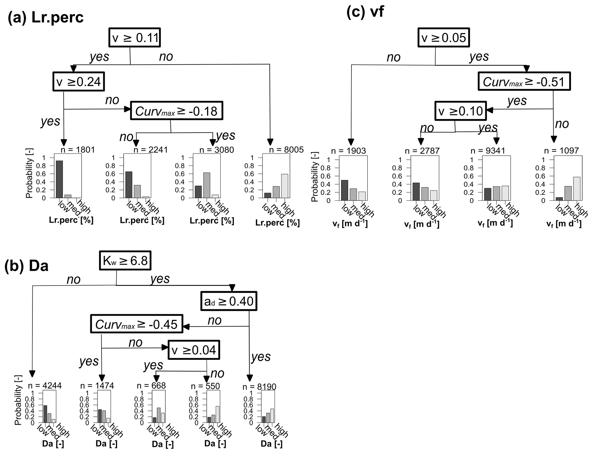
Figure 7CART decision trees for the response variables Lr.perc (accuracy = 0.66), Da (accuracy = 0.51) and vf (accuracy = 0.40). The trees are read from top to bottom, where the binary splits are followed to arrive at a histogram, illustrating the probability of a test sample having low, medium or high values (Table 3) for a certain response variable. The variables at the binary splits differ per response variable and consist of the median stream velocity (v; m d−1) and Curvmax for response variables Lr.perc and vf, while width coefficient Kw and depth exponent ad are identified additionally for Da. The prediction metrics for each of these classes and response variables are stated in Table C3.
These findings demonstrate that log (C)–log (Q) bending at the catchment outlet, together with the median velocity and the response of the width and the depth of a channel to discharge (parameters Kw, Kd, aw and ad) can help to classify the in-stream daily percentage of load removed Lr.perc, the Damköhler number Da and to a certain extent the uptake velocity vf. This conclusion depends of course on the initial assumptions of our model setup (e.g., linear land-to-stream loading vs. Q with a constant slope b and no dominant influence of waste water sources as well as no seasonality in uptake velocity vf). The velocity may be computed from the channel shape, discharge (Eq. 2c) and the topography with the channel shape parameters that are sometimes available from rating curve information or detectable from high-resolution satellite pictures. The CART models could help obtain an initial probability of removal efficiency in a river network, especially in a context where network-wide uptake measurements are scarce (Wollheim et al., 2017; Hensley et al., 2014), and physical, fully distributed models are not always feasible to apply (Boyer et al., 2006; Klemes, 1986). Although the CART models are developed using “only” the 13 German catchments included in the Monte Carlo analysis, in Sect. 3.3 and Table 4 we have shown that the output variability between the catchments (as a result of different catchment properties) is minor compared to the output variability within the catchments (due to the effect of the input parameter set), thus justifying the CART model use. Nevertheless, the prediction performance of these CART models might be influenced in unknown ways when applied to catchments with dissimilar catchment sizes, network structures or hydrological regimes.
In this study, we explore how low-frequency log (C)–log (Q) relationships, observed at a basin outlet, can display bending as a result of network-scale in-stream uptake processes. We established a parsimonious grid-based river network model for 13 distinct German catchments and investigated the influence of in-stream loading, transport and uptake parameters on the bending of log (C)–log (Q) relationships. Based on our exploratory analysis we conclude the following.
-
Noisy, multi-annual and low-frequency log (C)–log (Q) relationships at a basin outlet can be described as bent, and the amount of bending can be robustly quantified with the new Curvmax metric. Curvmax is temporally stable on multi-annual timescales and can be computed alongside existing log (C)–log (Q) descriptors, such as the slope of the linear regression model.
-
A bent log (C)–log (Q) relationship (Curvmax<0) at the basin outlet can arise from log–log linear land-to-stream C–Q relationships if uptake is present within the river network (vf≠0). This supports the hypothesis that more positive slopes under low flow (bent log (C)–log (Q) curves) are linked to biological concentration mediation in the stream (Moatar et al., 2017) and connects Curvmax (as a quantitative measure) to observations of increased removal efficiency under low flows (Wollheim et al., 2017). Our findings also stress the need to monitor the entire discharge range and capture low flows as well as high flows in a catchment.
-
The bending at the catchment outlet is primarily shaped by the channel geomorphological parameters aw and ad (exponents in the respective stream width and depth to discharge relationships, with Curvmax sensitivity indices KSmax equal to 0.62 and 0.51 and Spearman correlation coefficient ρ equaling 0.68 and 0.56, respectively) and less by the uptake velocity vf (KSmax=0.18, ), given that vf differs from zero. In the latter case Curvmax would equal zero, and the log (C)–log (Q) relationship would be solely shaped by the accumulation of upstream load. Thus, the change in reactive channel bed area with discharge (mediated by aw and ad) has a greater influence on the bending at the outlet than the biological removal capacity (here vf). Additionally we demonstrate that an a priori fixed aw might strongly affect the simulated C–Q dynamics at the basin outlet. This calls for a better representation of channel geomorphological parameters at stream networks to allow for better modeling assessments.
-
Curvmax at the basin outlet can be linked to the network-wide removal efficiency Lr.perc ( under certain conditions, generally showing that systems with more bending in their log (C)–log (Q) relationship are more efficient in terms of removal and vice versa. It is, however, clear that also cases with high bending () and low removal (Lr.perc<5.2 %, 0.9 % of all simulations) or low bending () with high removal (Lr.perc>63.0 %, 0.1 % of all simulations) exist that are imposed by respective higher and lower network-wide median velocities. This shows how the velocity, v, (calculated from the channel shape parameters aw, ad, Kw and Kd) may mediate the connection between Lr.perc and Curvmax and indicates that v should be considered when interpreting log (C)–log (Q) bending. Consequently, anthropogenic impacts in terms of channelization of river networks might lead to lower removal efficiencies.
-
Classification trees – like CART – can be useful for predicting low, median and high classes of response variables Lr.perc, the Damköhler number Da and vf. They provide useful insights on how catchments with low-frequency concentration and discharge time series (that are generally available) can reveal information on the upstream river network uptake performance.
To evaluate the generality of the results presented here, Curvmax should be calculated for concentration observations of a larger range of catchments and linked to the respective catchment properties. Properties such as light and stream ecological state can serve as proxies for uptake performance, and for example topographic gradient can be a proxy for network transport velocity. Finally, including conservative tracers in the analysis can be used to estimate loading scenarios. Such a data-driven exploration would further elucidate the linkages between nutrient uptake efficiency and low-frequency C and Q observations.
Calculation of c is performed as follows (Jawitz and Mitchell, 2011):
with
Stream channel wetted perimeter Pi [L] (where A is the cross-sectional area [L2]; RH [L] is the hydraulic radius; and wi [L], di [L] and vi [L T−1] are the local stream width, average depth and velocity, respectively) is calculated in Eq. (A2). Si [L L−1] is the stream bed slope, and n [–] is the Manning roughness coefficient that is equal to 0.03 for all simulations.
The load removed in a grid cell (Eq. 5) with the width and depth exponents aw and ad stated explicitly is calculated as follows:
The velocity in a grid cell (Eq. 2c) with the width and depth exponents aw and ad stated explicitly is calculated as follows:
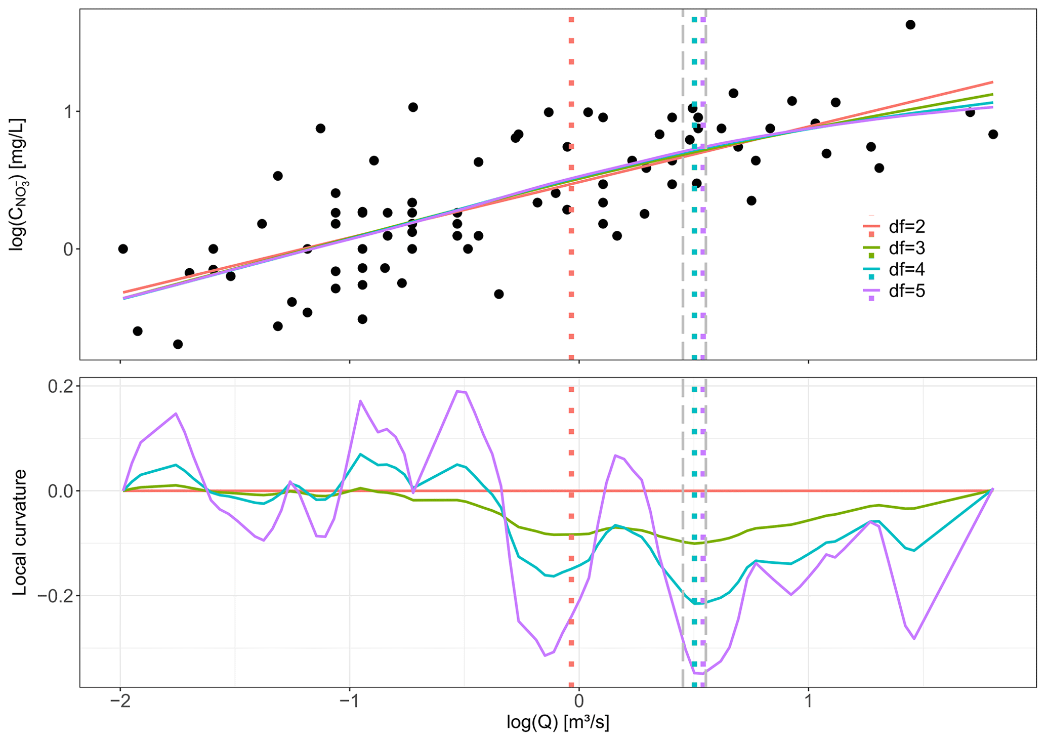
Figure B1Conceptual figure explaining Curvmax. The upper panel shows the log (C)–log (Q) relationship for Selke Meisdorf with the smoothed spline fits to these data for different degrees of freedom (df). The corresponding colors in the lower plot show then the local curvature values for these fitted smoothed splines. Also the log (Q) is indicated, for which the largest local curvature was found for each of the smoothed splines. Curvmax is then calculated as the largest local curvature value for a degree of freedom of 5 in this specific case as it is the largest degree of freedom that has the largest local curvature within Qm±0.05, with Qm equal to the log (Q) of the largest local curvature for df=3. Note that when Curvmax<0, the curve is concave, while for Curvmax>0 the curve is convex.
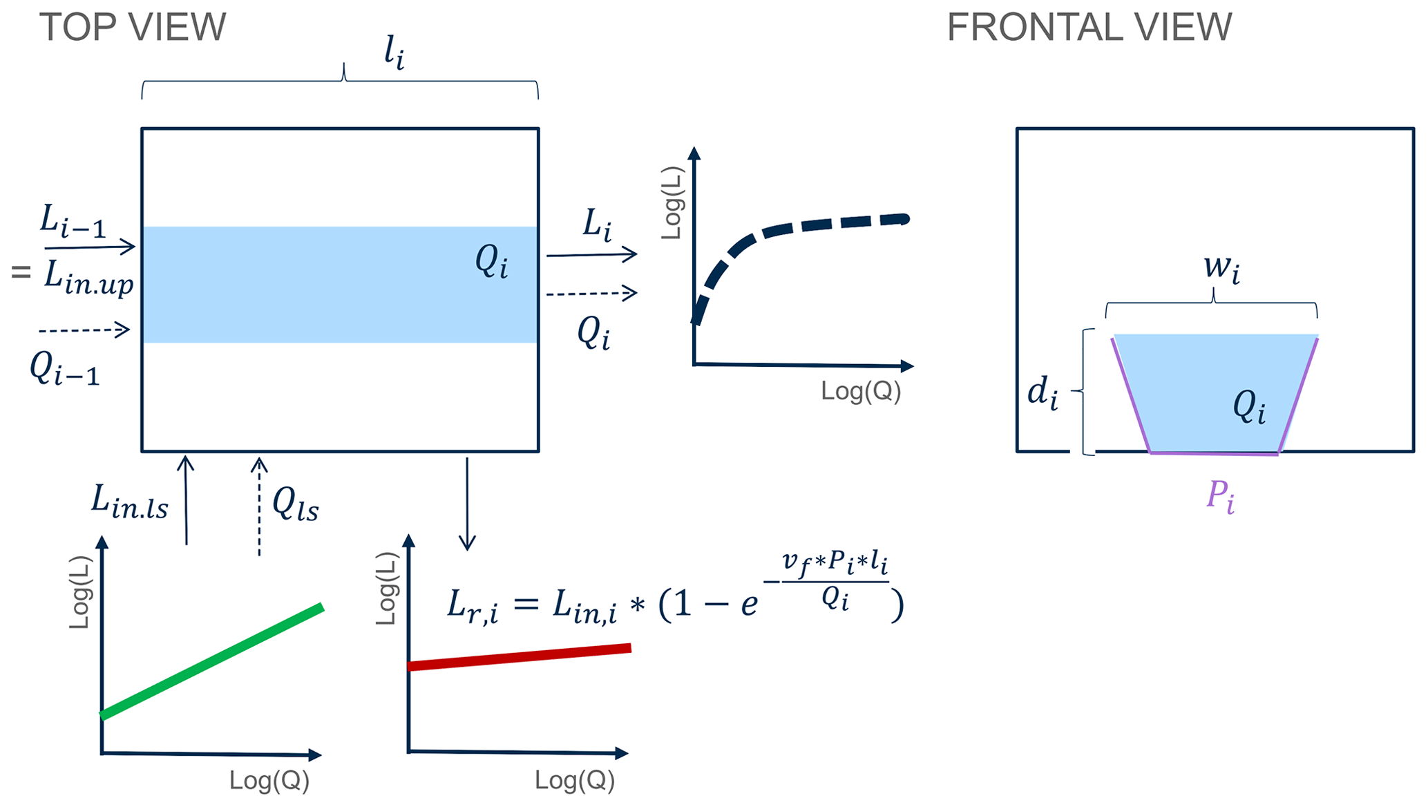
Figure B2Network model, illustrated for one grid cell. Here, the flow length through a grid cell i is li [L]; wi [L] and di [L] are the respective width and average depth of the reach, and Pi [L] is the corresponding stream channel wetted perimeter. The uptake velocity is denoted as vf. The local discharge Qi [L3 T−1] consists of upstream incoming discharge Qi−1 [L3 T−1] and land-to-stream runoff Qls [L3 T−1]. Similarly, the local load L [M T−1] consists of upstream incoming load Lin.up [M T−1] and the land-to-stream load Lin.ls [M T−1], where . Finally, the local load removed is denoted as Lr,i [M T−1].
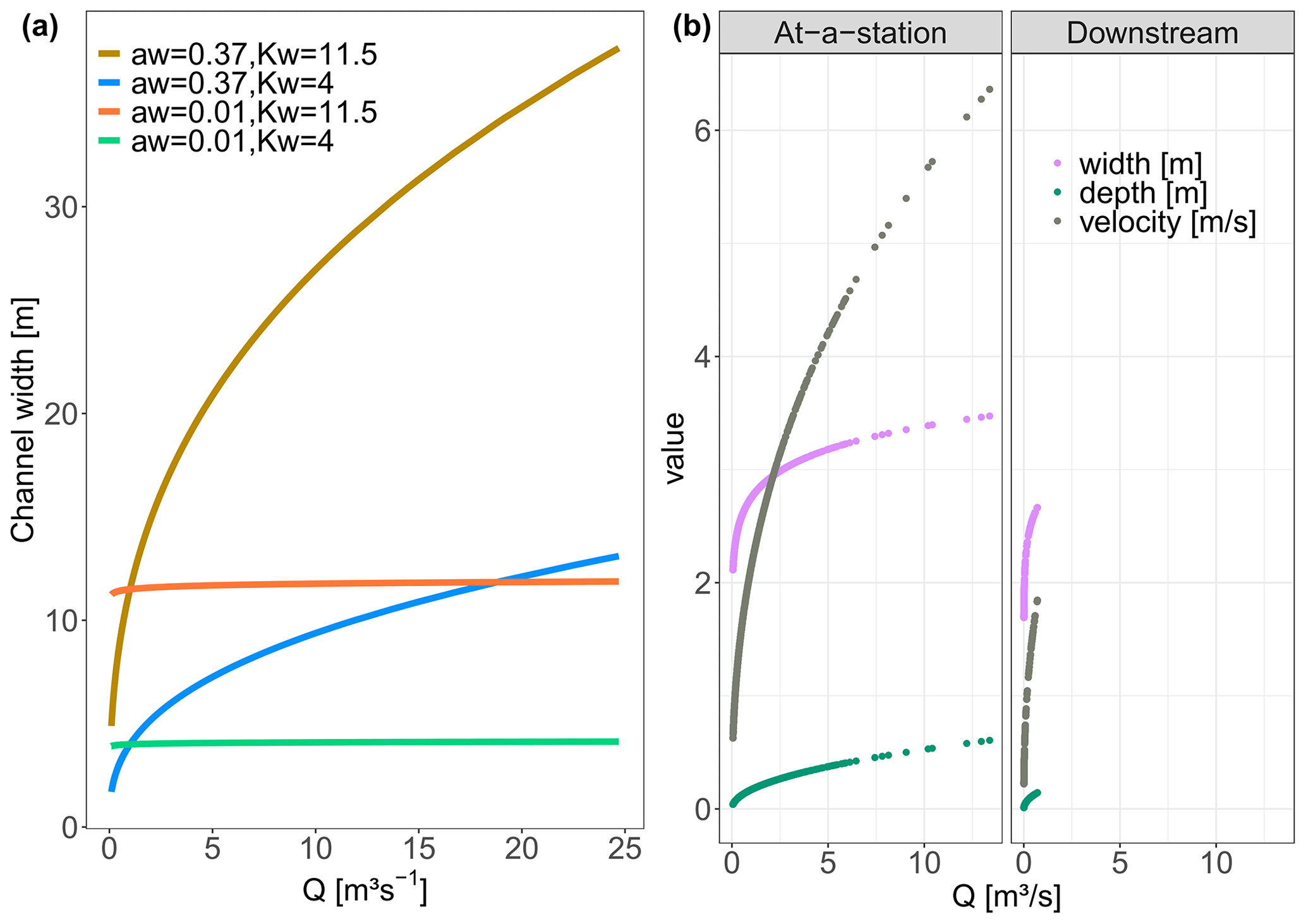
Figure B3(a) The effect of parameters aw and Kw on the channel width illustrated for the Q time series at the Selke Meisdorf station. (b) In the “At-a-station” panel the changes in velocity, depth and width with Q for grid cell B (Fig. 3) in the middle of the Selke network are evaluated. The “Downstream” panel, which considers all the network grid cells, shows the channel characteristics width, depth and velocity for a time t, with a Q of 0.70 m3 s−1 at the outlet. The values for the parameters aw, Kw, ad and Kd are the same for both scenarios (Table C1).
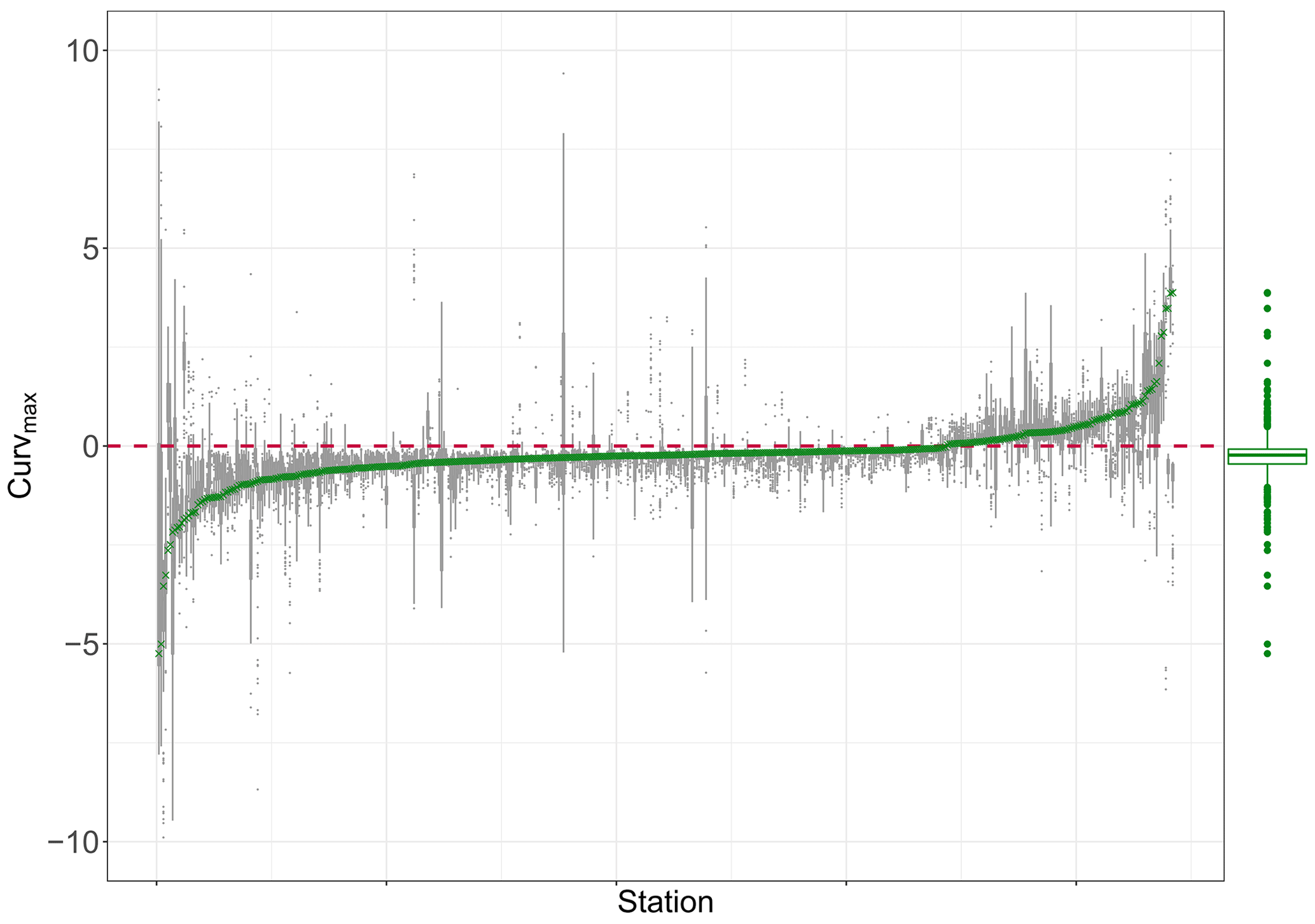
Figure B4Curvmax of nitrate log (C)–log (Q) data for 444 French monitoring stations arranged from left to right with increasing Curvmax (green crosses). For a given station, the gray boxplot represents the temporal robustness of this metric by subsampling 100 times from the original time series. The green boxplot indicates the range and distribution of all observed station Curvmax values.
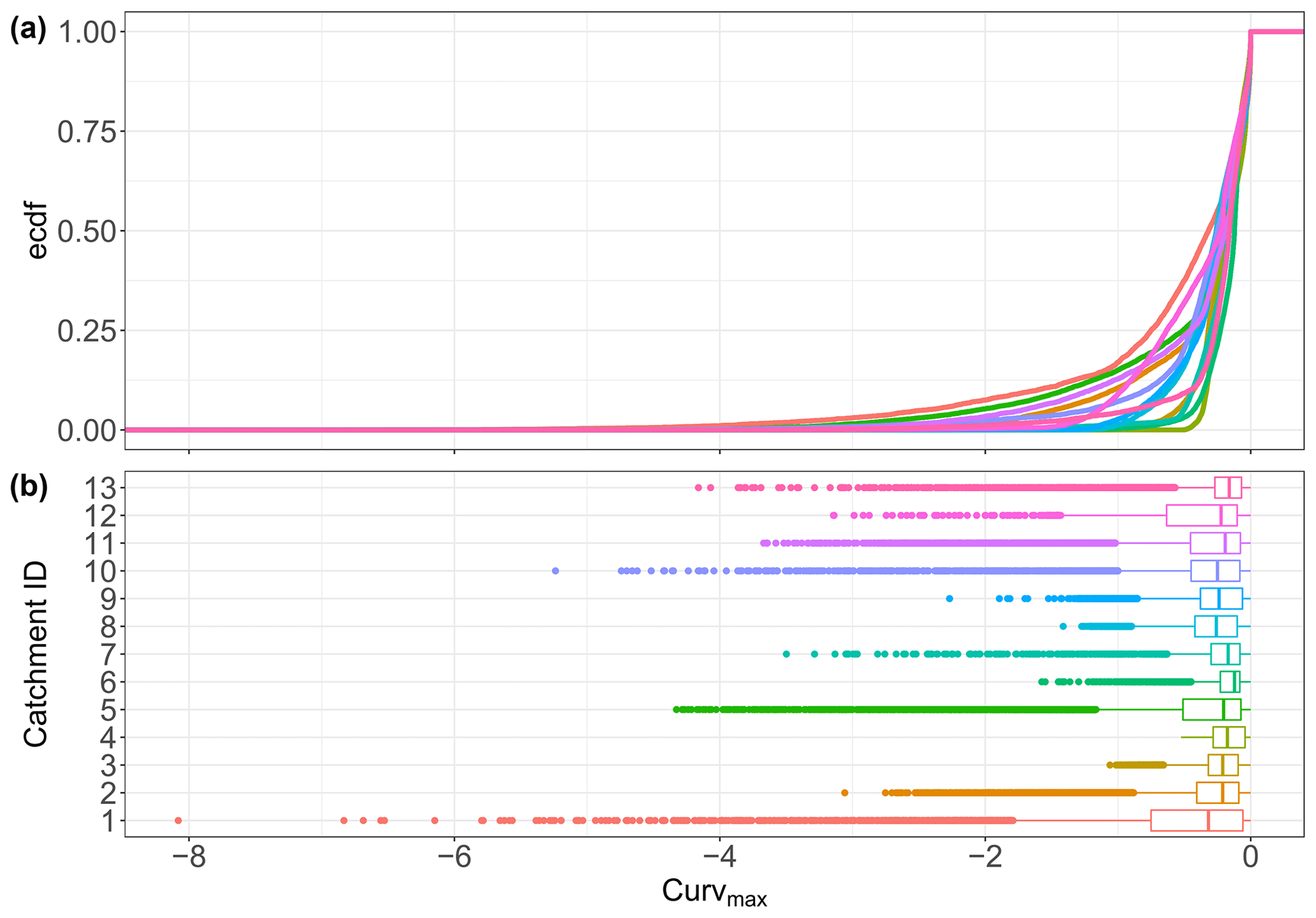
Figure B5Curvmax distributions resulting from running the same 11 107 input parameter combinations in each of the 13 catchments. Panel (a) shows the elemental cumulative distribution and (b) boxplots. None of the catchments have a normally distributed Curvmax set according to the Kruskal–Wallis (p<0.05) test.
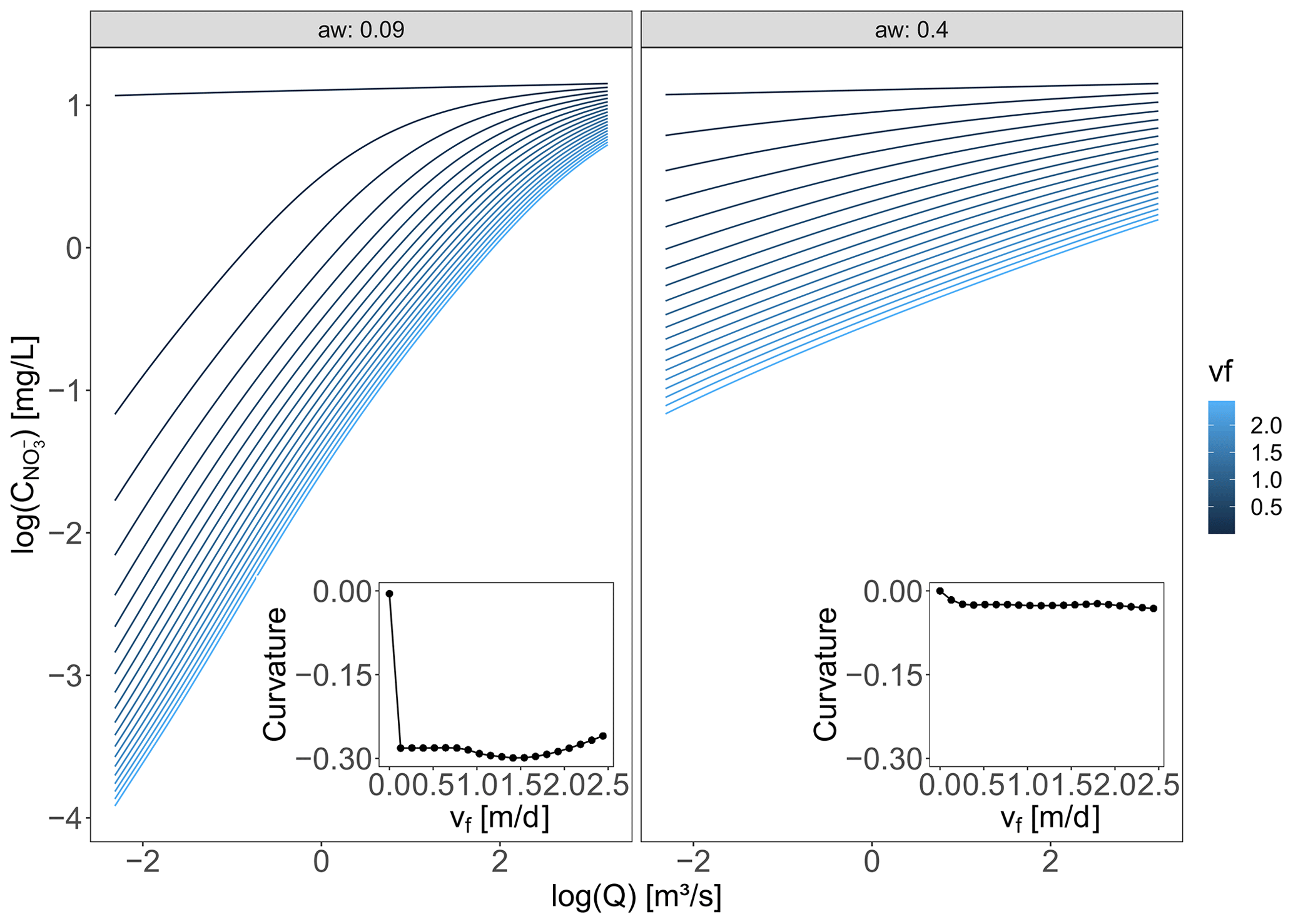
Figure B6Log(C)–log (Q) relationships and Curvmax for increasing uptake velocities (vf) resulting from network model simulations of the Selke Meisdorf catchment. As an example, two different aw values are displayed, and vf is varied from almost 0 to 2.5 m d−1 with the other parameter values as stated in Table C1.
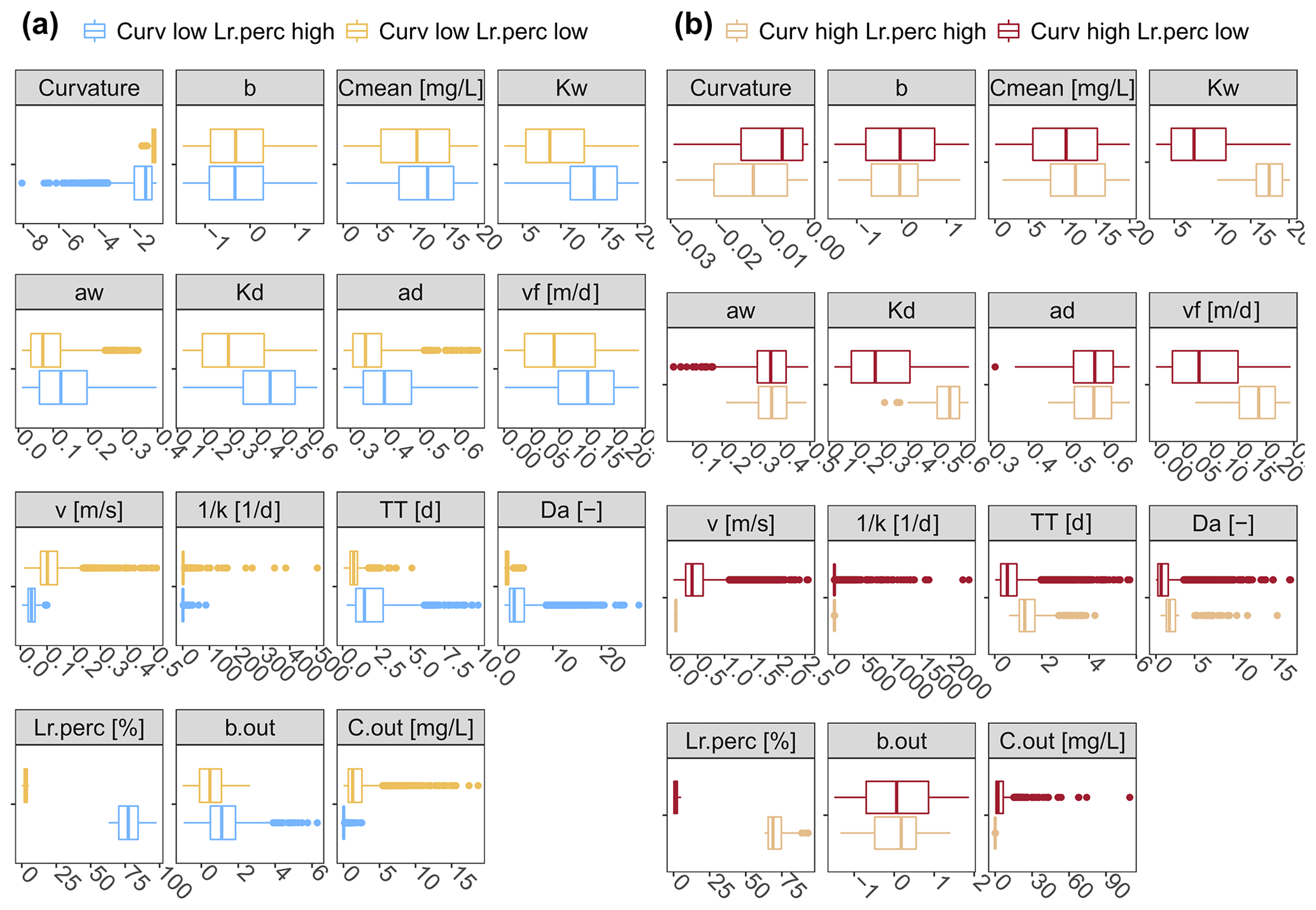
Figure B7Two specific cases of Fig. 6: (a) when Curvmax is low (high bending) and Lr.perc is low as opposed to high and (b) when Curvmax is high (low bending) and Lr.perc is high as opposed to low.

Table C2PAWN sensitivity indices KSmax for all the parameters and all the catchments, together with median and coefficients of variation (CV).

Table C3Performance statistics for each of the classes for the variables Lr.perc, Da and vf predicted by CART.
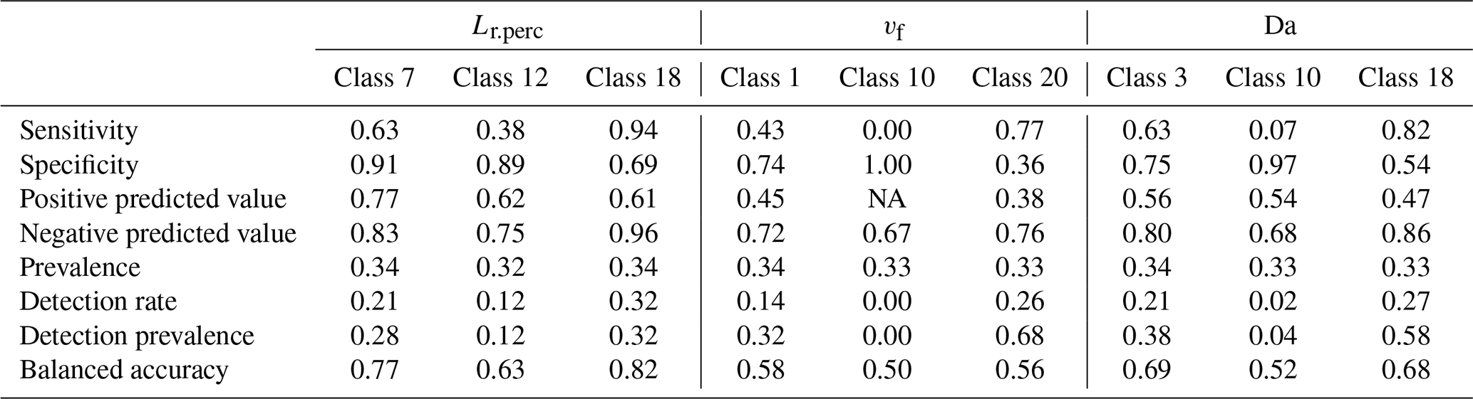
The network model code and the CurvMax function can be accessed at https://doi.org/10.4211/hs.da70a09dc6074242ada756c29d12dcb3 (Dehaspe, 2021).
The data we used were published by third parties and referenced in the text where appropriate, with complete access data in the reference list.
The supplement related to this article is available online at: https://doi.org/10.5194/hess-25-6437-2021-supplement.
JD and AM designed the study together with RK. JD developed the model code, carried out the simulations and interpreted them. FS provided help with the PAWN method. JD and AM prepared the manuscript draft, and all co-authors contributed to reviewing and editing the manuscript.
The authors declare that they have no conflict of interest.
Publisher's note: Copernicus Publications remains neutral with regard to jurisdictional claims in published maps and institutional affiliations.
This research was supported by funding from the InStream cohort and discussions with the participating scientists. Support to Fanny Sarrazin was provided by the Reduced Complexity Models project co-funded by the Helmholtz Association, and Fanny Sarrazin and Rohini Kumar acknowledge the Advanced Earth Modeling Capacity (ESM) project funded by the Helmholtz Association. The authors further thank Remi Dupas for providing the French nitrate CQ data, Pia Ebeling for the German catchment characteristics data and Nima Postanchi for his endless support.
The article processing charges for this open-access publication were covered by the Helmholtz Centre for Environmental Research – UFZ.
This paper was edited by Christian Stamm and reviewed by Wilfred Wollheim and one anonymous referee.
Abbott, B. W., Gruau, G., Zarnetske, J. P., Moatar, F., Barbe, L., Thomas, Z., Fovet, O., Kolbe, T., Gu, S., Pierson-Wickmann, A. C., Davy, P., and Pinay, G.: Unexpected spatial stability of water chemistry in headwater stream networks, Ecol. Lett., 21, 296–308, https://doi.org/10.1111/ele.12897, 2018.
Aguilera, R., Marcé, R., and Sabater, S.: Modeling nutrient retention at the watershed scale: Does small stream research apply to the whole river network?, J. Geophys. Res.-Biogeo., 118, 728–740, https://doi.org/10.1002/jgrg.20062, 2013.
Alexander, R. B., Smith, R. A., and Schwarz, G. E.: Effect of stream channel size on the delivery of nitrogen to the Gulf of Mexico, Nature, 403, 758–761, https://doi.org/10.1038/35001562, 2000.
Alexander, R. B., Böhlke, J. K., Boyer, E. W., David, M. B., Harvey, J. W., Mulholland, P. J., Seitzinger, S. P., Tobias, C. R., Tonitto, C., and Wollheim, W. M.: Dynamic modeling of nitrogen losses in river networks unravels the coupled effects of hydrological and biogeochemical processes, Biogeochemistry, 93, 91–116, https://doi.org/10.1007/s10533-008-9274-8, 2009.
Ameli, A. A., Beven, K., Erlandsson, M., Creed, I. F., McDonnell, J. J., and Bishop, K.: Primary weathering rates, water transit times, and concentration-discharge relations: A theoretical analysis for the critical zone, Water Resour. Res., 53, 942–960, https://doi.org/10.1002/2016wr019448, 2017.
Andreadis, K. M., Schumann, G. J. P., and Pavelsky, T.: A simple global river bankfull width and depth database, Water Resour. Res., 49, 7164–7168, https://doi.org/10.1002/wrcr.20440, 2013.
Basu, N. B., Rao, P. S. C., Thompson, S. E., Loukinova, N. V., Donner, S. D., Ye, S., and Sivapalan, M.: Spatiotemporal averaging of in-stream solute removal dynamics, Water Resour. Res., 47, W00J06, https://doi.org/10.1029/2010wr010196, 2011.
Bergstrom, A., McGlynn, B., Mallard, J., and Covino, T.: Watershed structural influences on the distributions of stream network water and solute travel times under baseflow conditions, Hydrol. Process., 30, 2671–2685, https://doi.org/10.1002/hyp.10792, 2016.
Bertuzzo, E., Helton, A. M., Hall, R. O., and Battin, T. J.: Scaling of dissolved organic carbon removal in river networks, Adv. Water Resour., 110, 136–146, https://doi.org/10.1016/j.advwatres.2017.10.009, 2017.
Beusen, A. H. W., Bouwman, A. F., Van Beek, L. P. H., Mogollón, J. M., and Middelburg, J. J.: Global riverine N and P transport to ocean increased during the 20th century despite increased retention along the aquatic continuum, Biogeosciences, 13, 2441–2451, https://doi.org/10.5194/bg-13-2441-2016, 2016.
Bieroza, M. Z., Heathwaite, A. L., Bechmann, M., Kyllmar, K., and Jordan, P.: The concentration-discharge slope as a tool for water quality management, Sci. Total Environ., 630, 738–749, https://doi.org/10.1016/j.scitotenv.2018.02.256, 2018.
Billen, G., Lancelot, C., and Meybeck, M.: N, P and Si retention along the aquatic continuum from land to ocean, in: Ocean Margin Processes in Global Change, 1st Edn., John Wiley & Sons, 19–44, 1991.
Birgand, F., Skaggs, R. W., Chescheir, G. M., and Gilliam, J. W.: Nitrogen removal in streams of agricultural catchments – A literature review, Crit. Rev. Env. Sci. Tec., 37, 381–487, https://doi.org/10.1080/10643380600966426, 2007.
Botter, G., Basso, S., Rodriguez-Iturbe, I., and Rinaldo, A.: Resilience of river flow regimes, P. Natl. Acad. Sci. USA, 110, 12925–12930, https://doi.org/10.1073/pnas.1311920110, 2013.
Bouwman, A. F., Bierkens, M. F. P., Griffioen, J., Hefting, M. M., Middelburg, J. J., Middelkoop, H., and Slomp, C. P.: Nutrient dynamics, transfer and retention along the aquatic continuum from land to ocean: towards integration of ecological and biogeochemical models, Biogeosciences, 10, 1–22, https://doi.org/10.5194/bg-10-1-2013, 2013.
Boyer, E. W., Alexander, R. B., Parton, W. J., Li, C. S., Butterbach-Bahl, K., Donner, S. D., Skaggs, R. W., and Del Gross, S. J.: Modeling denitrification in terrestrial and aquatic ecosystems at regional scales, Ecol. Appl., 16, 2123–2142, https://doi.org/10.1890/1051-0761(2006)016[2123:Mditaa]2.0.Co;2, 2006.
Breiman, L., Friedman, J., Stone, C. J., and Olshen, R. A.: Classification and Regression Trees, Chapman & Hall, London, 1984.
Canfield, D. E., Glazer, A. N., and Falkowski, P. G.: The evolution and future of Earth's nitrogen cycle, Science, 330, 192–196, https://doi.org/10.1126/science.1186120, 2010.
Dehaspe, J.: R codes for a stream network model and a C–Q bending metric, HydroShare [code], https://doi.org/10.4211/hs.da70a09dc6074242ada756c29d12dcb3, 2021.
Diamond, J. S. and Cohen, M. J.: Complex patterns of catchment solute-discharge relationships for coastal plain rivers, Hydrol. Process., 32, 388–401, https://doi.org/10.1002/hyp.11424, 2018.
Dingman, S. L.: Analytical derivation of at-a-station hydraulic–geometry relations, J. Hydrol., 334, 17–27, https://doi.org/10.1016/j.jhydrol.2006.09.021, 2007.
Doyle, M. W.: Incorporating hydrologic variability into nutrient spiraling, J. Geophys. Res., 110, G01003, https://doi.org/10.1029/2005jg000015, 2005.
Dupas, R., Musolff, A., Jawitz, J. W., Rao, P. S. C., Jäger, C. G., Fleckenstein, J. H., Rode, M., and Borchardt, D.: Carbon and nutrient export regimes from headwater catchments to downstream reaches, Biogeosciences, 14, 4391–4407, https://doi.org/10.5194/bg-14-4391-2017, 2017.
Dupas, R., Minaudo, C., and Abbott, B. W.: Stability of spatial patterns in water chemistry across temperate ecoregions, Environ. Res. Lett., 14, 074015, https://doi.org/10.1088/1748-9326/ab24f4, 2019.
Durand, P., Breuer, L., Johnes, P. J., Billen, G., Butturini, A., Pinay, G., and Wright, R.: Nitrogen processes in aquatic ecosystems, in: The European Nitrogen Assessment: Sources, Effects and Policy Perspectives, edited by: Sutton, M., Howard, C., Erisman, J., Billen, G., Bleeker, A., Grennfelt, P., van Grinsven, H., and Grizzetti, B., Cambridge University Press, Cambridge, 2011.
Ebeling, P.: CCDB – catchment characteristics data base Germany, HydroShare [data set], https://doi.org/10.4211/hs.0fc1b5b1be4a475aacfd9545e72e6839, 2020a.
Ebeling, P.: WQQDB – water quality metrics for catchments across Germany, HydroShare [data set], https://doi.org/10.4211/hs.9b4deeca259b4f7398ce72121b4e2979, 2020b.
Ebeling, P., Kumar, R., Weber, M., Knoll, L., Fleckenstein, J. H., and Musolff, A.: Archetypes and Controls of Riverine Nutrient Export Across German Catchments, Water Resour. Res., 57, e2020WR028134, https://doi.org/10.1029/2020WR028134, 2021.
EEA – European Environmental Agency: DEM over Europe from the GMES RDA project (EU-DEM, resolution 25 m) – version 1, October 2013, European Environmental Agency, EEA geospatial data catalogue, EEA [data set], https://sdi.eea.europa.eu/data/66fa7dca-8772-4a5d-9d56-2caba4ecd36a (last access: 14 March 2021), 2013.
Ehrhardt, S., Kumar, R., Fleckenstein, J. H., Attinger, S., and Musolff, A.: Trajectories of nitrate input and output in three nested catchments along a land use gradient, Hydrol. Earth Syst. Sci., 23, 3503–3524, https://doi.org/10.5194/hess-23-3503-2019, 2019.
Ensign, S. H. and Doyle, M. W.: Nutrient spiraling in streams and river networks, J. Geophys. Res.-Biogeo., 111, G04009, https://doi.org/10.1029/2005jg000114, 2006.
Ensign, S. H., McMillan, S. K., Thompson, S. P., and Piehler, M. F.: Nitrogen and phosphorus attenuation within the stream network of a coastal, agricultural watershed, J. Environ. Qual., 35, 1237–1247, https://doi.org/10.2134/jeq2005.0341, 2006.
ESRI: ArcGIS Desktop: Release 10, Environmental Systems Research Institute, Redlands, CA, 2011.
Fisher, S. G., Sponseller, R. A., and Heffernan, J. B.: Horizons in stream biogeochemistry: Flowpaths to progress, Ecology, 85, 2369–2379, https://doi.org/10.1890/03-0244, 2004.
Galloway, J. N., Schlesinger, W. H., Levy, H., Michaels, A., and Schnoor, J. L.: Nitrogen fixation: Anthropogenic enhancement-environmental response, Global. Biogeochem. Cy., 9, 235–252, https://doi.org/10.1029/95gb00158, 1995.
Godsey, S. E., Kirchner, J. W., and Clow, D. W.: Concentration-discharge relationships reflect chemostatic characteristics of US catchments, Hydrol. Process., 23, 1844–1864, https://doi.org/10.1002/hyp.7315, 2009.
Gomez-Velez, J. D., Harvey, J., Cardenas, M. B., and Kiel, B.: Denitrification in the Mississippi River network controlled by flow through river bedforms, Nat. Geosci., 8, 941–945, https://doi.org/10.1038/Ngeo2567, 2015.
Hall, R. O., Tank, J. L., Sobota, D. J., and Mulholland, P. J.: Nitrate removal in stream ecosystems measured by 15N addition experiments: Total uptake, Limnol. Oceanogr., 54, 653–665, https://doi.org/10.4319/lo.2009.54.3.0653, 2009.
Helton, A. M., Poole, G. C., Meyer, J. L., Wollheim, W. M., Peterson, B. J., Mulholland, P. J., Bernhardt, E. S., Stanford, J. A., Arango, C., Ashkenas, L. R., Cooper, L. W., Dodds, W. K., Gregory, S. V., Hall, R. O., Hamilton, S. K., Johnson, S. L., McDowell, W. H., Potter, J. D., Tank, J. L., Thomas, S. M., Valett, H. M., Webster, J. R., and Zeglin, L.: Thinking outside the channel: modeling nitrogen cycling in networked river ecosystems, Front. Ecol. Environ., 9, 229–238, https://doi.org/10.1890/080211, 2010.
Helton, A. M., Hall, R. O., and Bertuzzo, E.: How network structure can affect nitrogen removal by streams, Freshwater Biol., 63, 128–140, https://doi.org/10.1111/fwb.12990, 2018.
Hensley, R. T., Cohen, M. J., and Korhnak, L. V.: Inferring nitrogen removal in large rivers from high-resolution longitudinal profiling, Limnol. Oceanogr., 59, 1152–1170, https://doi.org/10.4319/lo.2014.59.4.1152, 2014.
Horton, R. E.: Erosional Development of Streams and Their Drainage Basins – Hydrophysical Approach to Quantitative Morphology, Geol. Soc. Am. Bull., 56, 275–370, https://doi.org/10.1130/0016-7606(1945)56[275:edosat]2.0.co;2, 1945.
Jarvie, H. P., Sharpley, A. N., Kresse, T., Hays, P. D., Williams, R. J., King, S. M., and Berry, L. G.: Coupling High-Frequency Stream Metabolism and Nutrient Monitoring to Explore Biogeochemical Controls on Downstream Nitrate Delivery, Environ. Sci. Technol., 52, 13708–13717, https://doi.org/10.1021/acs.est.8b03074, 2018.
Jawitz, J. W. and Mitchell, J.: Temporal inequality in catchment discharge and solute export, Water Resour. Res., 47, W00J14, https://doi.org/10.1029/2010wr010197, 2011.
Kadlec, R. H. and Reddy, K. R.: Temperature effects in treatment wetlands, Water. Environ. Res., 73, 543–557, https://doi.org/10.2175/106143001x139614, 2001.
Kiel, B. A. and Cardenas, M. B.: Lateral hyporheic exchange throughout the Mississippi River network, Nat. Geosci., 7, 413–417, https://doi.org/10.1038/Ngeo2157, 2014.
Kirchner, J. W., Feng, X., and Neal, C.: Fractal stream chemistry and its implications for contaminant transport in catchments, Nature, 403, 524–527, https://doi.org/10.1038/35000537, 2000.
Klemes, V.: Dilettantism in Hydrology – Transition or Destiny, Water Resour. Res., 22, S177–S188, https://doi.org/10.1029/WR022i09Sp0177S, 1986.
Kuhn, M.: caret: Classification and Regression Training, R package version 6.0-86, available at: https://CRAN.R-project.org/package=caret (last access: 16 December 2021), 2020.
Kumar, R., Hesse, F., Rao, P. S. C., Musolff, A., Jawitz, J. W., Sarrazin, F., Samaniego, L., Fleckenstein, J. H., Rakovec, O., Thober, S., and Attinger, S.: Strong hydroclimatic controls on vulnerability to subsurface nitrate contamination across Europe, Nat. Commun., 11, 6302, https://doi.org/10.1038/s41467-020-19955-8, 2020.
Kunz, J. V., Hensley, R., Brase, L., Borchardt, D., and Rode, M.: High frequency measurements of reach scale nitrogen uptake in a fourth order river with contrasting hydromorphology and variable water chemistry (Weisse Elster, Germany), Water Resour. Res., 53, 328–343, https://doi.org/10.1002/2016wr019355, 2017.
Langbein, W. B. and Leopold, L. B.: Quasi-Equilibrium States in Channel Morphology, Am. J. Sci., 262, 782–794, https://doi.org/10.2475/ajs.262.6.782, 1964.
Leopold, L. B. and Maddock, T.: The hydraulic geometry of stream channels and some physiographic implications, US Government Printing Office, Washington, DC, 1953.
Li, L., Sullivan, P. L., Benettin, P., Cirpka, O. A., Bishop, K., Brantley, S. L., Knapp, J. L. A., Meerveld, I., Rinaldo, A., Seibert, J., Wen, H., and Kirchner, J. W.: Toward catchment hydro-biogeochemical theories, WIREs Water, 8, e1495, https://doi.org/10.1002/wat2.1495, 2020.
Lindgren, G. A. and Destouni, G.: Nitrogen loss rates in streams: Scale-dependence and up-scaling methodology, Geophys. Res. Lett., 31, 1–4, https://doi.org/10.1029/2004gl019996, 2004.
Marcé, R. and Armengol, J.: Modeling nutrient in-stream processes at the watershed scale using Nutrient Spiralling metrics, Hydrol. Earth Syst. Sci., 13, 953–967, https://doi.org/10.5194/hess-13-953-2009, 2009.
Marcé, R., von Schiller, D., Aguilera, R., Martí, E., and Bernal, S.: Contribution of Hydrologic Opportunity and Biogeochemical Reactivity to the Variability of Nutrient Retention in River Networks, Global. Biogeochem. Cy., 32, 376–388, https://doi.org/10.1002/2017gb005677, 2018.
Marinos, R. E., Van Meter, K. J., and Basu, N. B.: Is the River a Chemostat: Scale Versus Land Use Controls on Nitrate Concentration-Discharge Dynamics in the Upper Mississippi River Basin, Geophys. Res. Lett., 47, e2020GL087051, https://doi.org/10.1029/2020gl087051, 2020.
McDonnell, J. J., Sivapalan, M., Vaché, K., Dunn, S., Grant, G., Haggerty, R., Hinz, C., Hooper, R., Kirchner, J., Roderick, M. L., Selker, J., and Weiler, M.: Moving beyond heterogeneity and process complexity: A new vision for watershed hydrology, Water Resour. Res., 43, W07301, https://doi.org/10.1029/2006wr005467, 2007.
Meybeck, M. and Moatar, F.: Daily variability of river concentrations and fluxes: indicators based on the segmentation of the rating curve, Hydrol. Process., 26, 1188–1207, https://doi.org/10.1002/hyp.8211, 2012.
Minaudo, C., Dupas, R., Gascuel-Odoux, C., Roubeix, V., Danis, P.-A., and Moatar, F.: Seasonal and event-based concentration-discharge relationships to identify catchment controls on nutrient export regimes, Adv. Water Resour., 131, 103379, https://doi.org/10.1016/j.advwatres.2019.103379, 2019.
Mineau, M. M., Wollheim, W. M., and Stewart, R. J.: An index to characterize the spatial distribution of land use within watersheds and implications for river network nutrient removal and export, Geophys. Res. Lett., 42, 6688–6695, https://doi.org/10.1002/2015gl064965, 2015.
Moatar, F., Abbott, B. W., Minaudo, C., Curie, F., and Pinay, G.: Elemental properties, hydrology, and biology interact to shape concentration-discharge curves for carbon, nutrients, sediment, and major ions, Water Resour. Res., 53, 1270–1287, https://doi.org/10.1002/2016wr019635, 2017.
Mueller, C., Musolff, A., Strachauer, U., Brauns, M., Tarasova, L., Merz, R., and Knöller, K.: Tomography of anthropogenic nitrate contribution along a mesoscale river, Sci. Total Environ., 615, 773–783, https://doi.org/10.1016/j.scitotenv.2017.09.297, 2018.
Mulholland, P. J. and Tank, J. L.: Can uptake length in streams be determined by nutrient addition experiments? Results from an interbiome comparison study, J. N. Am. Benthol. Soc., 21, 544–560, https://doi.org/10.2307/1468429, 2002.
Mulholland, P. J., Helton, A. M., Poole, G. C., Hall, R. O., Hamilton, S. K., Peterson, B. J., Tank, J. L., Ashkenas, L. R., Cooper, L. W., Dahm, C. N., Dodds, W. K., Findlay, S. E., Gregory, S. V., Grimm, N. B., Johnson, S. L., McDowell, W. H., Meyer, J. L., Valett, H. M., Webster, J. R., Arango, C. P., Beaulieu, J. J., Bernot, M. J., Burgin, A. J., Crenshaw, C. L., Johnson, L. T., Niederlehner, B. R., O'Brien, J. M., Potter, J. D., Sheibley, R. W., Sobota, D. J., and Thomas, S. M.: Stream denitrification across biomes and its response to anthropogenic nitrate loading, Nature, 452, 202–205, https://doi.org/10.1038/nature06686, 2008.
Musolff, A.: WQQDB – water quality and quantity data base Germany: metadata, Hydroshare, https://doi.org/10.4211/hs.a42addcbd59a466a9aa56472dfef8721, 2020.
Musolff, A., Fleckenstein, J. H., Rao, P. S. C., and Jawitz, J. W.: Emergent archetype patterns of coupled hydrologic and biogeochemical responses in catchments, Geophys. Res. Lett., 44, 4143–4151, https://doi.org/10.1002/2017gl072630, 2017.
Newbold, J. D., Elwood, J. W., Oneill, R. V., and Vanwinkle, W.: Measuring Nutrient Spiralling in Streams, Can. J. Fish. Aquat. Sci., 38, 860–863, https://doi.org/10.1139/f81-114, 1981.
O'Brien, J. M., Dodds, W. K., Wilson, K. C., Murdock, J. N., and Eichmiller, J.: The saturation of N cycling in Central Plains streams: 15N experiments across a broad gradient of nitrate concentrations, Biogeochemistry, 84, 31–49, https://doi.org/10.1007/s10533-007-9073-7, 2007.
Ocampo, C. J., Oldham, C. E., and Sivapalan, M.: Nitrate attenuation in agricultural catchments: Shifting balances between transport and reaction, Water Resour. Res., 42, W01408, https://doi.org/10.1029/2004wr003773, 2006.
Oldham, C. E., Farrow, D. E., and Peiffer, S.: A generalized Damköhler number for classifying material processing in hydrological systems, Hydrol. Earth Syst. Sci., 17, 1133–1148, https://doi.org/10.5194/hess-17-1133-2013, 2013.
Pennino, M. J., Kaushal, S. S., Beaulieu, J. J., Mayer, P. M., and Arango, C. P.: Effects of urban stream burial on nitrogen uptake and ecosystem metabolism: implications for watershed nitrogen and carbon fluxes, Biogeochemistry, 121, 247–269, https://doi.org/10.1007/s10533-014-9958-1, 2014.
Peterson, B. J., Wollheim, W. M., Mulholland, P. J., Webster, J. R., Meyer, J. L., Tank, J. L., Marti, E., Bowden, W. B., Valett, H. M., Hershey, A. E., McDowell, W. H., Dodds, W. K., Hamilton, S. K., Gregory, S., and Morrall, D. D.: Control of nitrogen export from watersheds by headwater streams, Science, 292, 86–90, https://doi.org/10.1126/science.1056874, 2001.
Pianosi, F. and Wagener, T.: A simple and efficient method for global sensitivity analysis based on cumulative distribution functions, Environ. Modell. Softw., 67, 1–11, https://doi.org/10.1016/j.envsoft.2015.01.004, 2015.
Pianosi, F. and Wagener, T.: Distribution-based sensitivity analysis from a generic input-output sample, Environ. Modell. Softw., 108, 197–207, https://doi.org/10.1016/j.envsoft.2018.07.019, 2018.
Pianosi, F., Sarrazin, F., and Wagener, T.: A Matlab toolbox for Global Sensitivity Analysis, Environ. Modell. Softw., 70, 80–85, https://doi.org/10.1016/j.envsoft.2015.04.009, 2015.
Pressley, A. N.: Elementary Differential Geometry, 1st Edn., Springer, London, https://doi.org/10.1007/978-1-84882-891-9, 2001.
R Core Team: R: A language and environment for statistical computing, R Foundation for Statistical Computing, Vienna, Austria, 2013.
Risse-Buhl, U., Anlanger, C., Kalla, K., Neu, T. R., Noss, C., Lorke, A., and Weitere, M.: The role of hydrodynamics in shaping the composition and architecture of epilithic biofilms in fluvial ecosystems, Water Res., 127, 211–222, https://doi.org/10.1016/j.watres.2017.09.054, 2017.
Rode, M., Halbedel Nee Angelstein, S., Anis, M. R., Borchardt, D., and Weitere, M.: Continuous In-Stream Assimilatory Nitrate Uptake from High-Frequency Sensor Measurements, Environ. Sci. Technol., 50, 5685–5694, https://doi.org/10.1021/acs.est.6b00943, 2016.
Runkel, R. L. and Bencala, K. E.: Transport of reacting solutes in rivers and streams, in: Environmental Hydrology, Kluwer Academic Publishers, Dordrecht, the Netherlands, 1995.
Schlesinger, W. H., Reckhow, K. H., and Bernhardt, E. S.: Global change: The nitrogen cycle and rivers, Water Resour. Res., 42, https://doi.org/10.1029/2005wr004300, 2006.
Seitzinger, S. P., Styles, R. V., Boyer, E. W., Alexander, R. B., Billen, G., Howarth, R. W., Mayer, B., and Van Breemen, N.: Nitrogen retention in rivers: model development and application to watersheds in the northeastern U. S. A., Biogeochemistry, 57–58, 199–237, https://doi.org/10.1023/A:1015745629794, 2002.
Seybold, E. and McGlynn, B.: Hydrologic and biogeochemical drivers of dissolved organic carbon and nitrate uptake in a headwater stream network, Biogeochemistry, 138, 23–48, https://doi.org/10.1007/s10533-018-0426-1, 2018.
Stream Solute Workshop: Concepts and Methods for Assessing Solute Dynamics in Stream Ecosystems, J. N. Am. Benthol. Soc., 9, 95–119, https://doi.org/10.2307/1467445, 1990.
Tunqui Neira, J. M., Andréassian, V., Tallec, G., and Mouchel, J.-M.: Technical note: A two-sided affine power scaling relationship to represent the concentration–discharge relationship, Hydrol. Earth Syst. Sci., 24, 1823–1830, https://doi.org/10.5194/hess-24-1823-2020, 2020.
Vanni, M. J.: Nutrient Cycling by Animals in Freshwater Ecosystems, Annu. Rev. Ecol. Syst., 33, 341–370, https://doi.org/10.1146/annurev.ecolsys.33.010802.150519, 2002.
Vanni, M. J. and McIntyre, P. B.: Predicting nutrient excretion of aquatic animals with metabolic ecology and ecological stoichiometry: a global synthesis, Ecology, 97, 3460–3471, https://doi.org/10.1002/ecy.1582, 2016.
Wei, T. and Simko, V.: R package “corrplot”: Visualization of a Correlation Matrix, version 0.84, GitHub, https://github.com/taiyun/corrplot (last access: 16 December 2021), 2017.
Winter, C., Lutz, S. R., Musolff, A., Kumar, R., Weber, M., and Fleckenstein, J. H.: Disentangling the impact of catchment heterogeneity on nitrate export dynamics from event to long-term time scales, Water. Resour. Res., 57, e2020WR027992, https://doi.org/10.1002/essoar.10503228.1, 2021.
Wollheim, W. M., Vörösmarty, C. J., Peterson, B. J., Seitzinger, S. P., and Hopkinson, C. S.: Relationship between river size and nutrient removal, Geophys. Res. Lett., 33, L06410, https://doi.org/10.1029/2006gl025845, 2006.
Wollheim, W. M., Peterson, B. J., Thomas, S. M., Hopkinson, C. H., and Vörösmarty, C. J.: Dynamics of N removal over annual time periods in a suburban river network, J. Geophys. Res., 113, G03038, https://doi.org/10.1029/2007jg000660, 2008.
Wollheim, W. M., Mulukutla, G. K., Cook, C., and Carey, R. O.: Aquatic Nitrate Retention at River Network Scales Across Flow Conditions Determined Using Nested In Situ Sensors, Water Resour. Res., 53, 9740–9756, https://doi.org/10.1002/2017wr020644, 2017.
Wollheim, W. M., Bernal, S., Burns, D. A., Czuba, J. A., Driscoll, C. T., Hansen, A. T., Hensley, R. T., Hosen, J. D., Inamdar, S., Kaushal, S. S., Koenig, L. E., Lu, Y. H., Marzadri, A., Raymond, P. A., Scott, D., Stewart, R. J., Vidon, P. G., and Wohl, E.: River network saturation concept: factors influencing the balance of biogeochemical supply and demand of river networks, Biogeochemistry, 141, 503–521, https://doi.org/10.1007/s10533-018-0488-0, 2018.
Yang, X., Jomaa, S., Buttner, O., and Rode, M.: Autotrophic nitrate uptake in river networks: A modeling approach using continuous high-frequency data, Water. Res., 157, 258–268, https://doi.org/10.1016/j.watres.2019.02.059, 2019.
Yang, X. Q., Jomaa, S., Zink, M., Fleckenstein, J. H., Borchardt, D., and Rode, M.: A New Fully Distributed Model of Nitrate Transport and Removal at Catchment Scale, Water Resour. Res., 54, 5856–5877, https://doi.org/10.1029/2017wr022380, 2018.
Zarnetske, J. P., Haggerty, R., Wondzell, S. M., and Baker, M. A.: Dynamics of nitrate production and removal as a function of residence time in the hyporheic zone, J. Geophys. Res., 116, G01025, https://doi.org/10.1029/2010jg001356, 2011.