the Creative Commons Attribution 4.0 License.
the Creative Commons Attribution 4.0 License.
 | 16 Dec 2021
Calibrating 1D hydrodynamic river models in the absence of cross-section geometry using satellite observations of water surface elevation and river width
Silja Westphal Christensen
Peter Bauer-Gottwein
Hydrodynamic modeling has been increasingly used to simulate water surface elevation which is important for flood prediction and risk assessment. Scarcity and inaccessibility of in situ bathymetric information have hindered hydrodynamic model development at continental-to-global scales. Therefore, river cross-section geometry is commonly approximated by highly simplified generic shapes. Hydrodynamic river models require both bed geometry and roughness as input parameters. Simultaneous calibration of shape parameters and roughness is difficult, because often there are trade-offs between them. Instead of parameterizing cross-section geometry and hydraulic roughness separately, this study introduces a parameterization of 1D hydrodynamic models by combining cross-section geometry and roughness into one conveyance parameter. Flow area and conveyance are expressed as power laws of flow depth, and they are found to be linearly related in log–log space at reach scale. Data from a wide range of river systems show that the linearity approximation is globally applicable. Because the two are expressed as power laws of flow depth, no further assumptions about channel geometry are needed. Therefore, the hydraulic inversion approach allows for calibrating flow area and conveyance curves in the absence of direct observations of bathymetry and hydraulic roughness. The feasibility and performance of the hydraulic inversion workflow are illustrated using satellite observations of river width and water surface elevation in the Songhua river, China. Results show that this approach is able to reproduce water level dynamics with root-mean-square error values of 0.44 and 0.50 m at two gauging stations, which is comparable to that achieved using a standard calibration approach. In summary, this study puts forward an alternative method to parameterize and calibrate river models using satellite observations of river width and water surface elevation.
- Article
(16856 KB) - Full-text XML
- BibTeX
- EndNote


Hydrodynamic modeling of rivers is important for quantitative assessment of river flow and water level dynamics and, critically, for risk assessment and flood prediction. It is widely used for many applications, such as estimates of hydraulic parameters (e.g., water surface elevation – WSE, longitudinal profile, velocity), flood forecasting, inundation estimation, risk assessment, river maintenance, etc. (Andreadis and Schumann, 2014; Bates et al., 2014; Bierkens, 2015; Blöschl et al., 2015; Jiang et al., 2020). Nowadays, in the era of big data, earth observation data sets, cloud computing, and complex modeling platforms are available for better simulations of WSE at multiple scales (Fleischmann et al., 2019; Gleason and Durand, 2020; Ward et al., 2015).
Traditional hydrodynamic modeling approaches require a detailed river channel bathymetry, which is usually represented by a set of cross-section shapes, distributed along the river reach of interest. There are, however, only a limited number of rivers for which the surveyed geometry is available. The challenge that arises in many studies is how to approximate the channel geometry. This is a common problem which the scientific community faces. A common approach is to parameterize channel geometry as a simple shape, e.g., a rectangle or triangle (Garambois et al., 2017; Jiang et al., 2019; Neal et al., 2012; Schneider et al., 2017). Instead of rectangular or triangular shapes, Dingman (2007) and Neal et al. (2015) used a power function (bankfull width and depth are required) to represent channel shape variability between the limiting cases of rectangular and triangular shape. However, Neal et al. (2015) used a cross-section geometry which did not vary along the channel. Similar parameterizations of cross-section shapes were used in Mejia and Reed (2011), and the effect of assumed shapes on simulated flows was investigated. Some studies estimated river bathymetry using global DEMs combined with an assumed simplified shape (e.g., rectangle) of the submerged portion of the river. Domeneghetti (2016) used DEM data to infer the river bathymetry based on width–elevation relationships of high flow and low flow. Similarly, a few studies infer bathymetry from water surface height and width by fitting the relationship between the two. Obviously, the success of this approach depends on the channel exposure (Mersel et al., 2013). Moreover, combinations of remote sensing data and empirical statistical relationships or data assimilation approaches have also been used to infer effective bathymetry (Brisset et al., 2018; Dey et al., 2019; Durand et al., 2008; Fonstad and Marcus, 2005; Grimaldi et al., 2018; Larnier et al., 2021; Legleiter, 2015; Moramarco et al., 2019; Schaperow et al., 2019). For instance, Durand et al. (2008) estimated bathymetric depth and slope by assimilating synthetic WSE data from the Surface Water and Ocean Topography (SWOT) mission into the LISFLOOD-FP hydrodynamic model. Larnier et al. (2021) also applied data assimilation to infer effective bathymetry from synthetic SWOT altimetry measurements within an inverse framework. Here, we do not comprehensively review bathymetry estimation using upcoming SWOT mission data. Instead, we refer the reader to Biancamaria et al. (2016) and Gleason and Durand (2020) for a broader overview.
In addition to the channel bathymetry, channel roughness is another factor that is important for simulating flow dynamics with sufficient accuracy (Bates et al., 2014; Neal et al., 2015). Usually, a uniform value is adopted to represent channel/floodplain roughness although large heterogeneity of river roughness exists in most cases (Annis et al., 2020; Jiang et al., 2020; Pappenberger et al., 2007; Schumann et al., 2007). When calibrating channel geometry parameters along with roughness parameters, strong parameter correlation appears between cross-section shape (wetted perimeter) and hydraulic roughness (Jiang et al., 2019). That is, the roughness parameter will be “effective”, not only representing the friction but also compensating for inaccurate geometry, which affects the hydraulic resistance through the wetted perimeter. Therefore, there is a trade-off between roughness and geometry parameters, which has been widely reported (see Garambois and Monnier, 2015, and references therein).
In order to reduce parameter correlation in hydraulic inverse problems, we put forward a method to parameterize and calibrate 1D river models in a different way. Instead of roughness and geometry, flow area and conveyance curves as functions of flow depth are estimated in an inverse modeling workflow. In this way, only the dependence of area and conveyance on flow depth is estimated, regardless of the detailed channel shape and roughness. This paper illustrates this approach for the calibration of a 1D MIKE HYDRO River model (DHI, 2017) to simulate WSE dynamics, using satellite observations of WSE and river width. The novelty is to use power-law relationships between flow-area/conveyance and flow depth in a hydraulic inversion without detailed cross-section data or assumption of any specific cross-section shape. Therefore, this approach is fundamentally different from previous studies, and it provides an alternative way for hydrodynamic model calibration.
2.1 Theoretical background
Flow in open channels can be described by the continuity equation and momentum equation, known as the Saint-Venant equations (Chow, 1959):
where A is the cross-section area; Q is the discharge; d is the flow depth; S0 is the slope of the channel bottom; Sf is the friction slope; g is the gravity acceleration; t is time and x is chainage, i.e., the distance along the channel.
Equations (1) and (2) comprise the 1D dynamic wave model. In the absence of cross-section geometry, there are five unknowns in this model, i.e., two variables (Q and d) and three unknown values (A, S0, and Sf), which are functions of further parameters as specified below. To solve for Q and d, information about channel geometry and friction slope is required. Flow area A and channel slope S0 can be obtained once the bathymetry is known. The friction slope Sf can be approximated using the Manning formula or the Chézy formula (Chow, 1959).
Here, we express friction slope as a function of conveyance (K) and discharge (Q) using Manning's equation:
where n is the Manning roughness coefficient, and R is the hydraulic radius. The conveyance is a measure of water carrying capacity of a cross-section (Chow, 1959).
Substituting for Sf, the momentum equation is written as
This version of the momentum equation (Eq. 5) indicates that, in steady state (for both kinematic wave and diffusive wave), the calibration is much more sensitive to K(d) than to A(d), and A(d) appears only when the flow accelerates or decelerates.
2.2 Parameterization of flow area and conveyance curves
Equations (1) and (5) are two equations with still five unknowns, i.e., two variables (Q and d), and three unknown values (A, S0, and K). However, K and A are related to flow depth, d. If K and A can be expressed as functions of d, Q and d can be solved for, given the slope S0 but without the need for detailed information on cross-section shape and roughness. The hydraulic geometry relations are widely used to relate the water surface width, average depth, and average velocity to discharge since it was introduced by Leopold and Maddock in 1953 (Bjerklie et al., 2005; Dingman, 2007; Ferguson, 1986; Gleason, 2015; Leopold and Maddock, 1953). Dingman (2007) has derived explicit equations for the exponent and coefficients in the power-law function, explaining the variation of hydraulic geometry in different rivers. In some way analogous to the at-a-station power law of hydraulic geometry, power laws that relate flow area A and conveyance K to flow depth d of a cross-section can be written, respectively, as (Chow, 1959; Garbrecht, 1990)
where a, β, c, and δ are empirical coefficients; H and Z0 are WSE and channel datum, i.e., water surface elevation for zero flow.
Transforming Eqs. (6) and (7) into log–log space, we can write the following linear relationships:
where α=log (a) and γ=log (c). This relationship is investigated for several rivers to show its validity for real-world rivers. Between the rivers, the width ranges over 3 orders of magnitude. Note that these six rivers are used simply due to the availability of cross-section data (see a map of rivers and cross-sections in Fig. A1 in Appendix A). Strong positive linear relationships are revealed by plotting the logarithmic A–d and K–d pairs for any given cross-section below bankfull depth (Fig. 1). A discontinuity may occur if a significant flood plain exists as in the case of the Yellow River (Fig. 1d). Chow (1959) and Garbrecht (1990) suggested using separate functions to approximate the hydraulic properties below and above bankfull depth. In this initial study, one single power law is used. Note that the conveyance changes with the Manning's coefficient, but the linear relationship holds (Fig. A2). To calculate conveyance, spatially varying, randomly distributed Manning's coefficient values ranging between 0.015 and 0.05 are used to mimic real-world rivers instead of unrealistic uniform values along the whole reach. A uniform Manning's coefficient results in a much stronger linear relationship (Figs. A2 and A3).
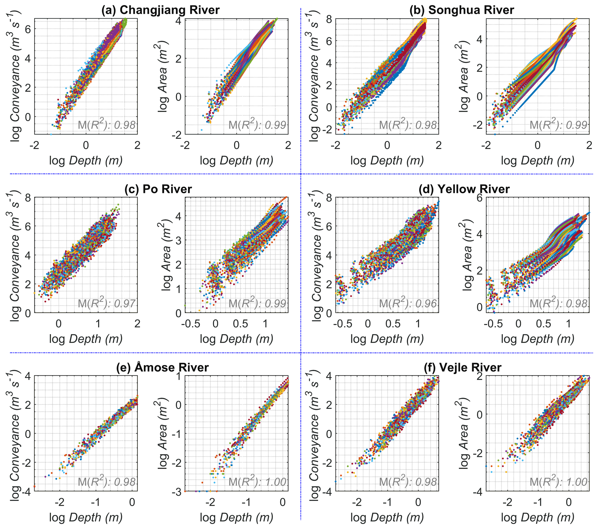
Figure 1Plots of flow area and conveyance against flow depth in log–log space. In each plot, dots of the same color are from one certain cross-section. Linear relationships between logarithmic-area/conveyance and depth are estimated for each cross-section, i.e., in an “at-a-station” manner. The median value of slopes of linear regression is given in each plot. In total, there are 60, 70, 335, 98, 51, and 165 cross-sections spaced at 2.5 km, 6 m, 1 km, 8 km, 150 m, and 300 m, respectively, for (a) Changjiang, (b) Songhua, (c) Po, (d) Yellow, (e) Åmose, and (f) Vejle rivers. Please refer to Fig. A1 for a detailed map. Note that Manning's coefficient used for calculation of conveyance for each cross-section is randomly generated between 0.015 and 0.05.
However, there are four more parameters (i.e., α, β, γ, δ) for each cross section to be estimated. Due to the linear nature of logarithmic pairs of (A–d) and (K–d), a linear relationship can be derived between the A–d and K–d curves for each individual cross-section. The mathematical derivations are given in Appendix A (Eqs. A1–A4). Unfortunately, the linear relationships are varying with cross-sections; therefore, many coefficients (intercepts and slopes of the linear function as shown in Eqs. A2 and A4) have to be determined. By fitting a linear function to the cross-section parameter pairs (α–δ and β–γ) derived from observed data at the reach scale as shown in Fig. 2, the flow area and conveyance curves for all cross-sections can be connected by
It should be noted that the linear relationships (i.e., Eqs. 9 and 10) are only valid at river reach scale instead of individual cross-sections. In this way, we can simplify the hydraulic inverse problem by tying the parameters together, i.e., halving the number of fitting parameters. Interestingly, p1, p2, p3, and p4 are nearly constant and independent of rivers although marginal deviations exist (Fig. A4). As shown in Fig. 2, when pooling cross-sections of all rivers together, a clear linear trend shows up for both α–γ and β–δ. This indicates that parameters p2 and p4 should vary in a very narrow range around 1.0 for all rivers; parameters p1 and p3 should be allowed to slightly vary around −1.4 and −0.7 to adapt to individual rivers. Thus, there are two spatially varying parameters (i.e., γ, δ) and four uniform parameters (i.e., p1–p4) in addition to the bed datum Z0, from which the bed slope S0 is calculated, which have to be constrained in order to solve Q and d. Therefore, a new parameterization of a river model can be written as
with p1, p2, p3, and p4 close to −1.4, −0.7, 1.0, and 1.0, respectively.

Figure 2Linear relationship between and . Each dot represents one cross-section of a certain river. Dots of the same color are from the same river. Manning's coefficient for each cross-section is randomly generated between 0.015 and 0.05. Note that the best-fit line for each river is slightly different. The relationship using a uniform Manning's coefficient of 0.03 is also given in Fig. A3. Individual fitting lines are shown in Fig. A4.
2.3 Parameter calibration
Hydraulic parameter calibration is essentially an inverse problem that is often solved using the least squares approach. Considering the large number of parameters (p1, p2, p3, and p4, and spatially varying Z0, γ, and δ), regularization is used to stabilize the ill-posed problem (Pereverzyev et al., 2006; Schmidt, 2005). In this work, the Tikhonov-type regularization is applied, and the objective function is formulated following Aster et al. (2018):
where X is vector containing the parameters γ, δ, p1, p2, p3, p4, and z; λ is a weighting factor balancing the regularization and data fitting error; w is a weighting factor balancing the fitness of water level and width; hs, ho, Nh, and σh are simulated water level, observed water level, number of water levels, and the uncertainty of observed water level; bs, bo, Nb, and σb are simulated width (calculated as the derivative of flow area with respect to depth in the model), observed width, number of widths, and the uncertainty of observed width; λγ, λδ, , , , and are regularization parameters; σγ, σδ, , , , , and σz are the a priori standard deviations indicating how uncertain the parameters are a priori; N is the number of cross-sections; and L is the first-order regularization roughening matrix, which is a finite-difference approximation to the first derivative of the model:
In this case study, the weighting factor λ is set as 0.8 based on a trial-and-error method. The weighting factor w is set to 0.5; i.e., water level and river width observations are equally important. The uncertainties of water level and width are 0.5 and 99 m according to Jiang et al. (2017) and Yang et al. (2020), respectively. The a priori standard deviations of σγ and σδ are 0.7 and 0.4, respectively, which are similar for relatively large rivers (see γ and δ distributions in Fig. S2). The a priori standard deviations of p1, p2, p3, and p4 are chosen as 0.02, 0.01, 0.02, and 0.01, respectively, given that those parameters vary slightly (see Figs. A3 and A4). The datum Z0 is the sum of parameter z and a constant value which is estimated from the average water level subtracting the depth of 5 m. The a priori standard deviation of z is 0.5 m. The regularization parameters, i.e., λγ, λδ, , , , and , are empirically set as 0.1, 0.1, 0.15, 0.15, 0.15, and 0.15, respectively, to achieve appropriate smoothness.
We iteratively optimize the objective function (Eq. 15) with the Levenberg–Marquardt (LM) algorithm (Marquardt, 1963) combined with Broyden's rank-one update to approximate the Jacobian (Broyden, 1965; Madsen et al., 2004). We use an implementation of the method provided by the Immoptibox toolbox (Nielsen and Völcker, 2010). Given that LM finds a local minimum and cannot guarantee the global minimum, an ensemble of 10 calibrations is carried out with different initial guesses to avoid convergence to a local minimum. For each calibration, the number of model runs is around 200. The time consumed for this optimization is a few hours (1–4 h). The calibrations were conducted on a Windows Server 2016 (Intel® Xeon® Gold 6154 CPU at 3 GHz, 2993 MHz) using four cores.
The calibration is implemented in MATLAB. C# scripts are used to modify and dump MIKE Hydro River parameters and simulation results. The power-law relationships are an integral part of the MIKE Hydro River model. Specifically, for each iteration of the optimization, the updated parameters by LM algorithm and the calculated flow area and conveyance relationships are passed to a C# script that updates the setup of the MIKE Hydro River model. Then the model is executed, and the results are passed on to MATLAB. Essentially, by optimizing Eq. (15) using satellite-derived observations of WSE and river width, we calibrate the two curves, i.e., the relationships between flow-area/conveyance and depth as described by Eqs. (13) and (14) for each cross-section along the reach.
To test whether this approach is able to reproduce realistic flow area and conveyance curves as well as WSE using remote sensing data, we use the Songhua river as a test site. Below are the descriptions of the test site, data sets, model setup, and calibration procedures.
3.1 Study site
Songhua river is the longest tributary of the Amur (or Heilong Jiang) and one of the largest rivers in the world. It allows for testing the approach using satellite data sets, such as altimetry and imagery, which will be available simultaneously from the future SWOT mission (Biancamaria et al., 2016).
The river has two sources, i.e., the Nenjiang and Second Songhua rivers, originating from the Greater Khingan Range in the north and the Paektu Mountain in the south, respectively, and drains an area of 556 800 km2. At Sanchahe, two tributaries merge to form the Songhua river. It runs 840 km northeastward before draining into the Amur river (Songliao River Conservancy Commission, 2004, 2015). In this study, we focus on the middle reach of the Songhua river, between Harbin and Jiamusi (Fig. 3). The reasons why we selected this reach are twofold: firstly, it is wide enough (700 m on average) to have high-quality altimetry data as shown in a previous study (Jiang et al., 2017), and secondly, we have access to in situ data of several hydrometric stations across this region. This reach covers an area of 138 500 km2 and stretches 433 km long. The elevation difference of this reach is about 45 m, resulting in an average slope of 0.1 m km−1. The first 222 km part flows through hilly terrain with a gentle slope of 0.05 m km−1, while the downstream reach is narrower and deeper. The mean discharge at the downstream end is about 1175 m3 s−1. The river is frozen in winter and reaches its maximum flow in summer.
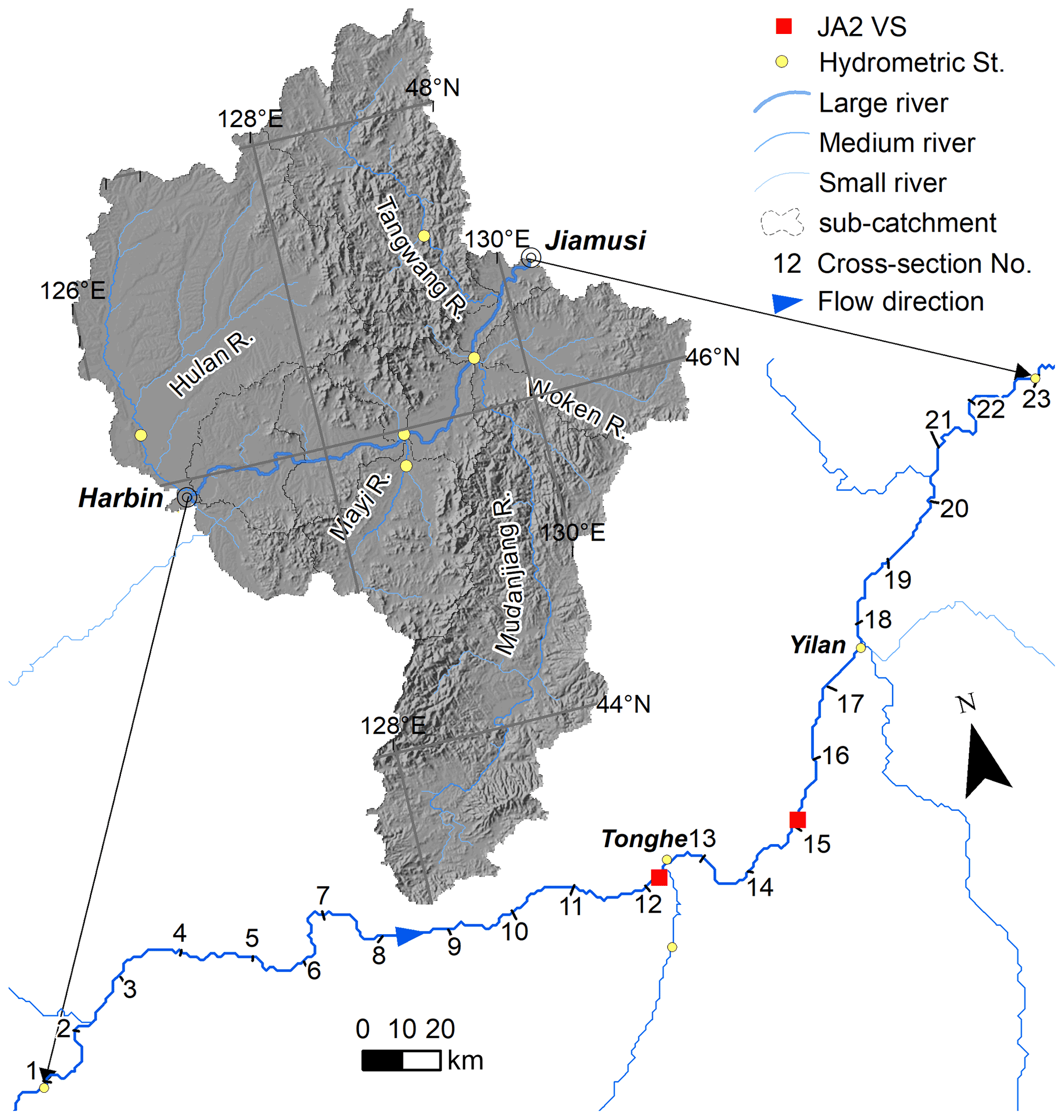
Figure 3Overview of the study area. The studied reach is 433 km long between Harbin and Jiamusi. There are five major tributaries recharging the main river. There are 23 cross-sections evenly distributed along this reach as shown in the lower map.
3.2 Data sets and model setup
A 1D river model is built using the MIKE HYDRO River software (DHI, 2017). The first step is to define the river network, cross-sections, and boundary conditions. The river network is set up using the center line of the reach, while 23 cross-sections are equally distributed along the 433 km reach as in Jiang et al. (2019). The daily discharge at Harbin hydrometric station is used as the upstream boundary, while a uniform flow depth rating curve is set as downstream boundary. Inflows of three tributaries are from gauging records, while remaining tributary inflows are simulations from a hydrological model (Jiang et al., 2019). The only available in situ surveyed cross-sections are from the late 1990s. These “real” area curves are only used to validate the calibration results.
WSE and river width derived from CryoSat-2 altimetry and Landsat imagery are used as observations in the calibration. CryoSat-2 altimetry is distinctive due to several features, most importantly the orbit configuration. Specifically, CryoSat-2 with its drifting ground track pattern results in an entirely different sampling pattern. The small inter-track spacing of 7.5 km enables dense sampling of rivers and thus provides longitudinal water level profiles. Although these profiles are not snapshots of river level at a given time, they are still useful for resolving local hydraulic characteristics (Jiang et al., 2019; Schneider et al., 2018). CryoSat-2 observations are the same as those used in Jiang et al. (2019), covering the period 2010–2014. Widths are extracted using the RivWidthCloud algorithm in Google Earth Engine (Yang et al., 2020). We used Landsat 5 and Landsat 8 images, and we selected images avoiding cloud cover and obtained an even distribution in time. Specifically, if the river is cloud-free in a given image, it is selected regardless of the cloudiness of other parts. Images collected from December to early April are excluded. In total, 37 Landsat 5 images and 15 Landsat 8 images are used and provided 10 022 individual width observations. The temporal and spatial distribution of WSE and width observations is shown in Fig. B1.
For the purpose of validation, gauging records of water level and discharge at Tonghe and Yilan (Fig. 3) are collected. Moreover, WSE data sets derived from Jason-2 at two virtual stations (Fig. 3) are also included for extensive validation. Because the river is completely frozen, altimetry does not provide realistic WSE observations during the winter. Therefore, we only consider the ice-free period (April to October) in this study. To compare results with the previously published calibration approach (e.g., simultaneous calibration of roughness and cross-section shape parameters), we also extract model simulations from our previous work (Jiang et al., 2019). Specifically, water level simulations from model calibration S1 (refer to Jiang et al., 2019) are used for a fair comparison given that both calibrations use the same amount of CryoSat-2 WSE data.
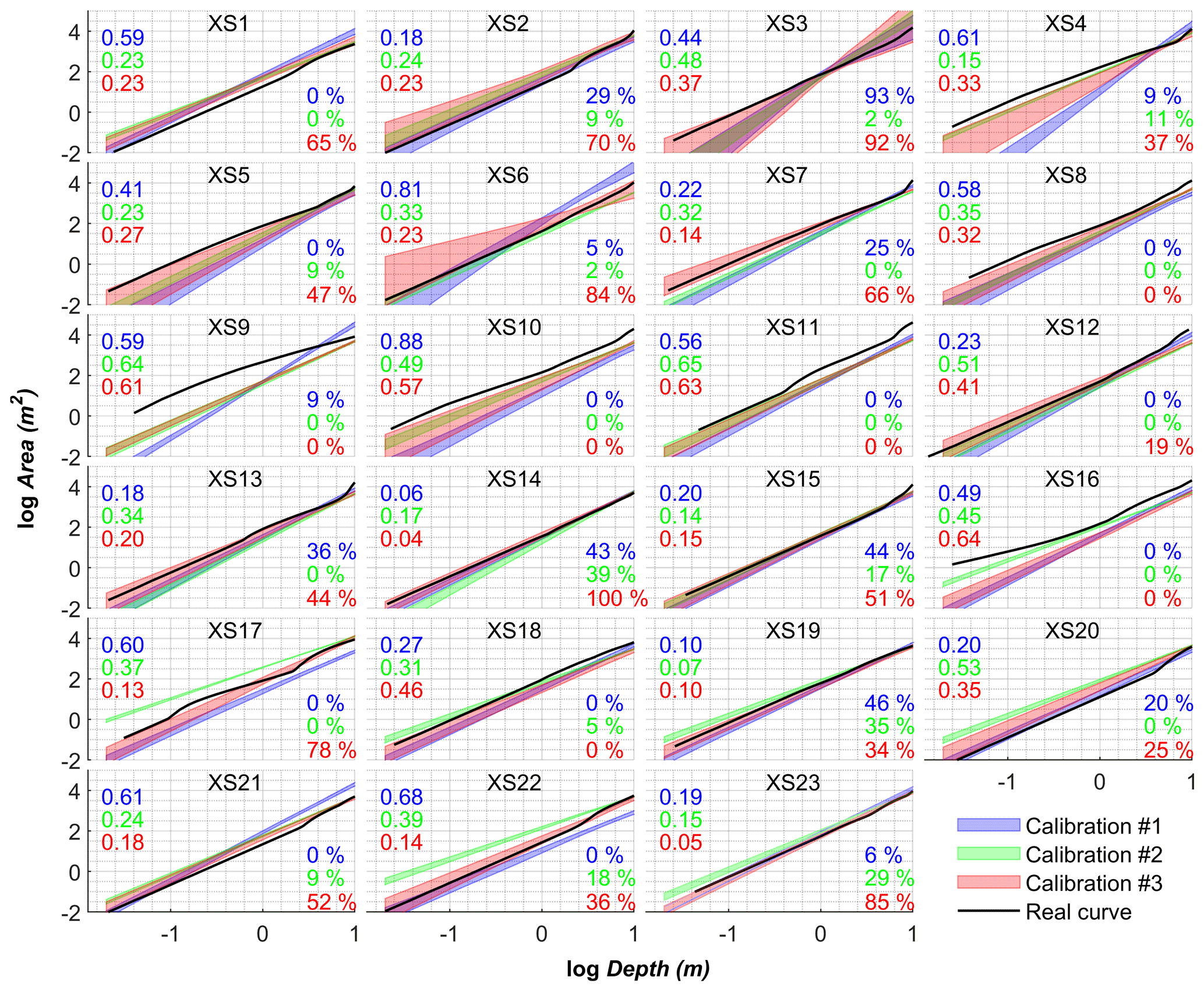
Figure 4Calibrated area–depth curves at 23 cross-sections (number is given in each plot). Three scenarios are shown, i.e., calibration with water surface elevation data only (calibration #1), river width only (calibration #2), and both water surface elevation and width (calibration #3), respectively. Please refer to Table 1 for more information. The color band represents the mean ± standard deviation based on an ensemble of 10 calibrations. RMSE and coverage (percentage of real data falling into the calibrated interval) of calibrated curves against real data are reported on the left and right sides of each plot, respectively. Font color is consistent with the curve color.
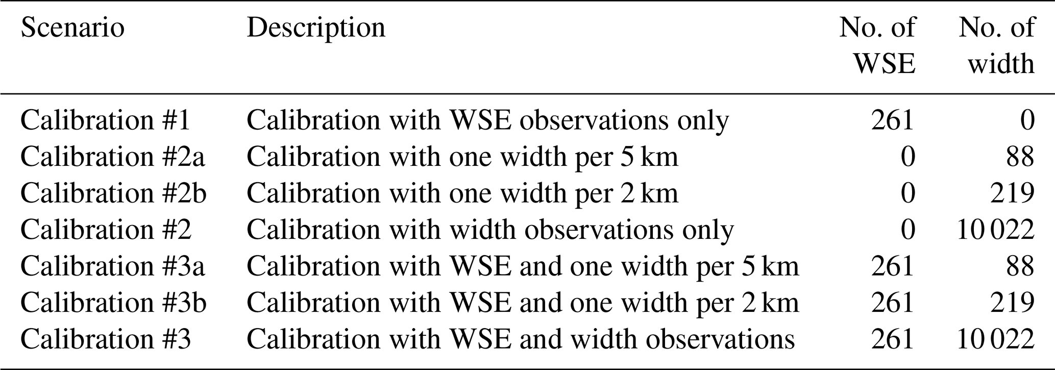
Table 1Details of the calibration scenarios with different data sets.
3.3 Calibration scenarios
To test the capability of different data sets to constrain model parameters, three basic scenarios are used based on the type of data sets. That is, calibration #1 uses altimetry-derived WSE only, calibration #2 uses imagery-derived width only, and calibration #3 uses both WSE and width. Given that width observations are of very high spatial resolution (30 m interval), three scenarios of width observations are also designed (Table 1). Specifically, width is sampled at coarse spatial resolution by randomly selecting one observation for each 2 or 5 km reach regardless of the timing. Given that only 261 observations of WSE are available, no further exploration of the effect of WSE data is performed. Therefore, in total, we test seven scenarios of observations to calibrate the model (Table 1).
Results prove that it is possible to calibrate spatially varying area–depth curves solely using satellite data sets. Figure 4 depicts the calibrated area–depth curves at 23 cross-sections under the three scenarios. Two metrics are used to evaluate the performance alongside the plots. RMSE describes the error of the calibrated log Area vs. log Depth relationship, and coverage is defined by the percentage of real data that fall within the confidence interval. Compared to the curves derived from surveyed cross-sections, the calibrated ones are reasonably close at most locations. Most of the largest errors occur at cross-sections 4–6, where the Dadingzishan reservoir (chainage 20–90 km) is located and not modeled. Interestingly, both WSE alone and river width alone are able to constrain the model to a certain degree (Fig. 4). However, calibration #1 (WSE only) has slightly larger spread especially for small depths. The average RMSE and coverage are 0.42 and 16 %. Calibration #2 (width only) tends to overestimate flow area, which is significant for downstream cross-sections. The corresponding average RMSE and coverage are 0.34 and 8 %. Calibration #3 (both WSE and width) shows the best match (smaller RMSE and larger coverage) with the observed cross-sections (Fig. 4). Moreover, very dense observations of width (#2 and #3) do not improve the calibration results compared to less dense ones (#2a and #2b, #3a and #3b), although calibrations #2 and #3 result in narrower confidence intervals (Figs. B2 and B3).
Figure 5 shows the performance of each calibration scenario in terms of accuracy of simulated water level. Similarly, models calibrated with either WSE (calibration #1) or width (calibration #2) can reproduce WSE with similar RMSE at two gauging stations. However, calibration #2 shows larger RMSEs and wider ranges than calibration #1, especially at the Yilan station. In contrast, calibration #3 is more stable, resulting in smaller RMSEs and narrower ranges. This is in line with the well-calibrated area–depth curves at cross-sections (XS12, XS13, XS17, XS18) nearby the two gauging stations (refer to Fig. 3 for the locations). Regarding the scenarios using width observations, the RMSE values of calibrations #2a and #2b are very spread out (i.e., a wide range), indicating that models are not well-constrained. This is evidenced by the poorly calibrated area–depth curves (e.g., wider color bands of XS17 and XS18) shown in Fig. B2.
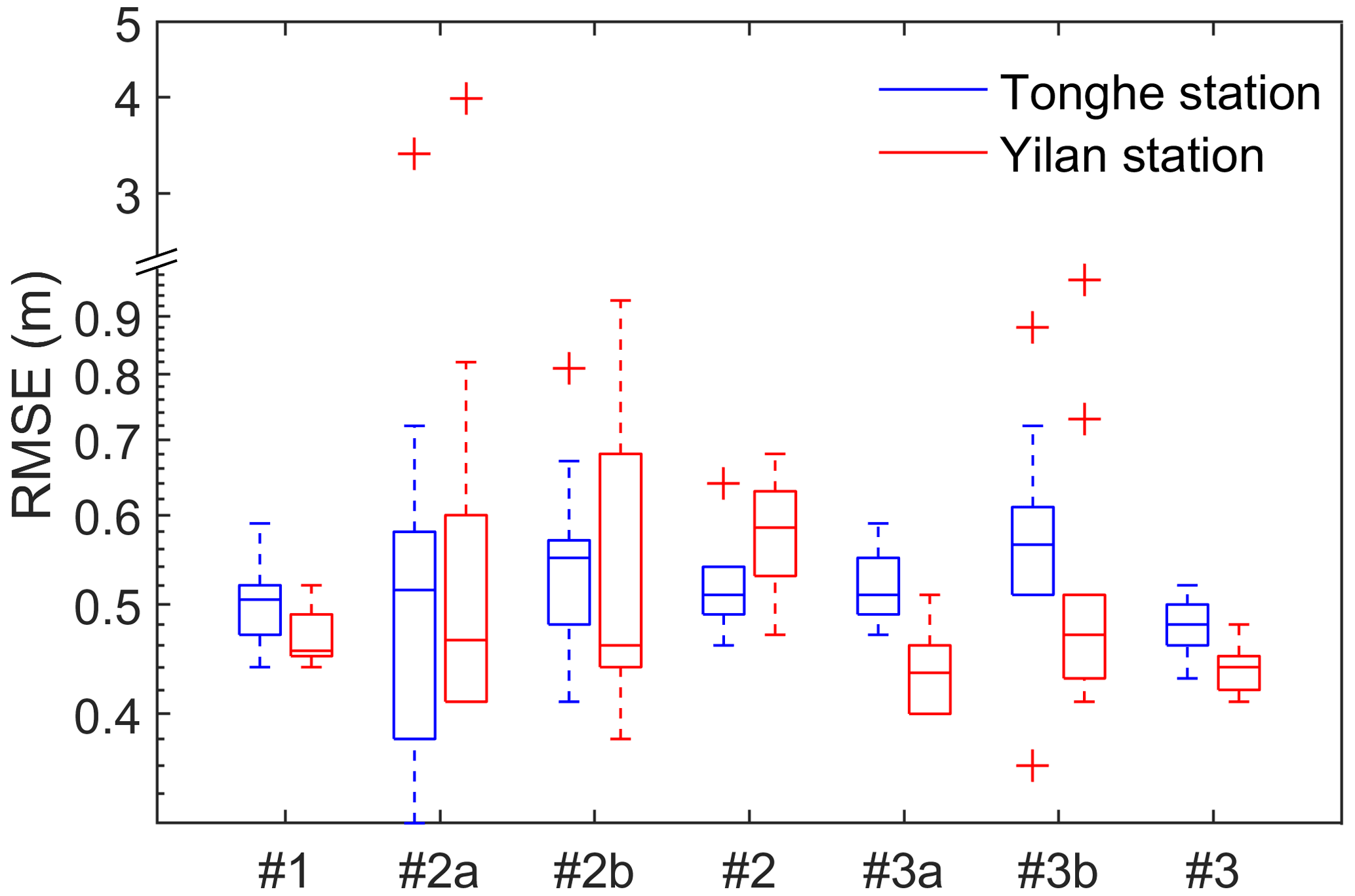
Figure 5Boxplots of evaluations of simulated water level against in situ gauging records at two gauging stations. Calibration scenarios indicated on the x axis are referred to Table 1. Note that the y axis is in log scale. Note that the statistics for each scenario are computed from the 10 calibration runs with different starting points.
The calibrated model can reproduce the WSE reasonably well when compared with independent data sets. Figure 6 shows simulated WSE using calibrated curves shown in Fig. 4. Overall, the accuracy of simulation is acceptable. The RMSE is about 50 and 44 cm at Tonghe and Yilan stations, respectively. The accuracy is comparable to what was achieved using a different approach, which simultaneously calibrates cross-section shape parameters and roughness (Jiang et al., 2019). A careful comparison indicates that the simulations are slightly better than those reported in Jiang et al. (2019) for low WSE (Fig. 6). Compared to Yilan, Tonghe shows slightly higher RMSE (Fig. 6) due to the underestimation of the extremely high WSE in 2013, although the simulated discharge matches in situ observations well (Fig. C1). This can be well explained by the calibrated curves. The curves at two neighboring cross-sections (XS12 and XS13) show deviations from the curves derived from surveyed cross-sections beyond bankfull depth (upward curves as shown in Fig. 4). Evaluation at the two virtual stations also shows good agreements. However, the model simulation is better than Jason-2 observations except during the 2013 flood when compared to the hydrograph of an adjacent gauging station, i.e., Tonghe station (Fig. 6).
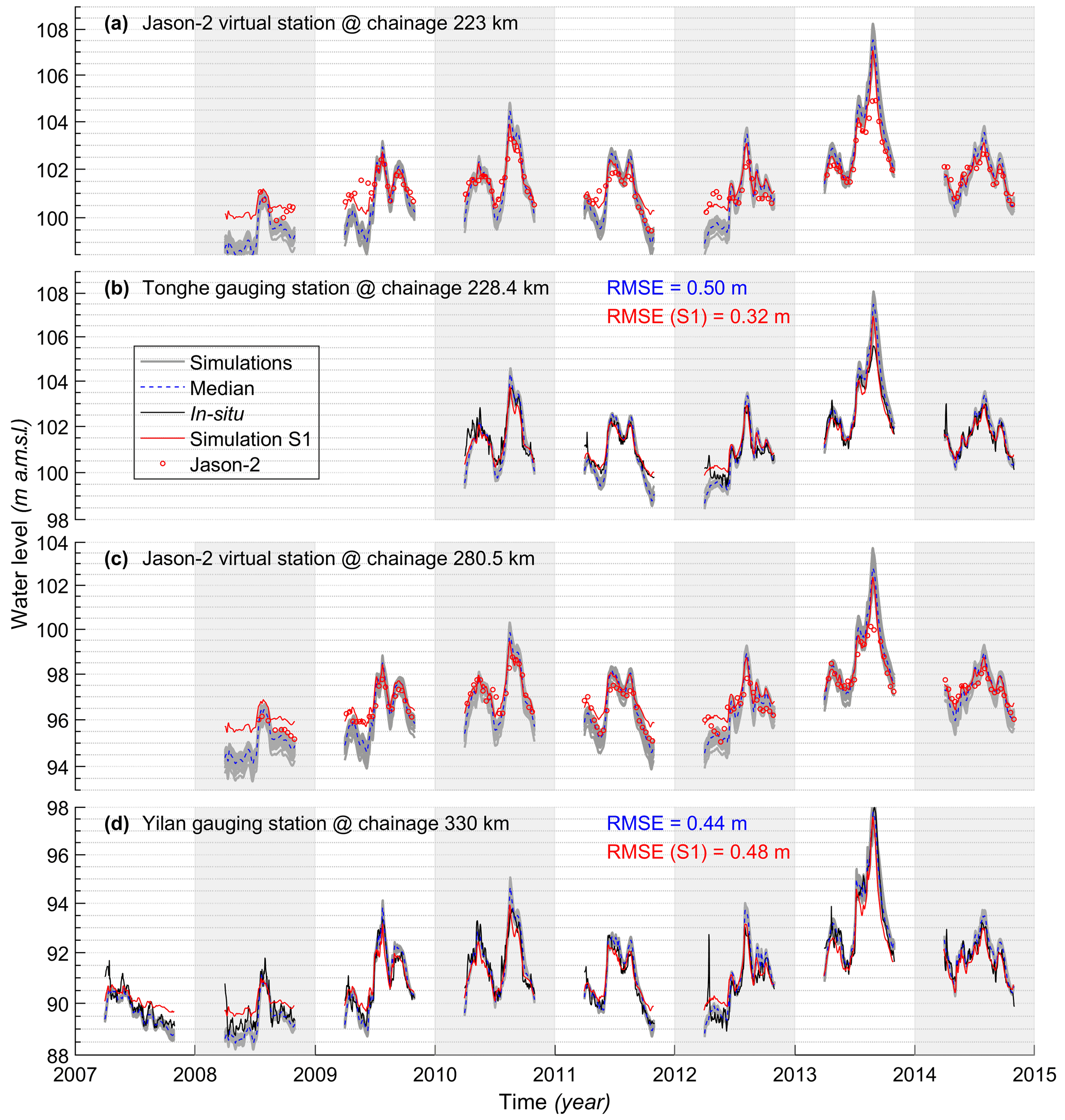
Figure 6Validation of simulated water level (non-frozen periods) at four stations. Panels (a) and (c) are water levels at two virtual stations, i.e., data derived from Jason-2 altimetry. Panels (b) and (d) are from two stream gauging stations. Simulation from previous model calibrated using different strategy (i.e., simultaneous calibration of roughness and cross-section shape parameters; simulation S1 in Jiang et al., 2019) is also shown for comparison. Note that, in each plot, results of the median and individual simulations of an ensemble of 30 calibrations (#1, #2, and #3) are shown.
5.1 The value of altimetry and imagery in model calibration
Satellite altimetry data and imagery data have been increasingly used to calibrate hydrologic and hydrodynamic river models (Domeneghetti et al., 2014; Jiang et al., 2019; Liu et al., 2015; Michailovsky et al., 2012; Milzow et al., 2011; Sun et al., 2010). However, joint use of imagery and altimetry for hydrodynamic modeling is not common practice. For our case study, models calibrated with either river width only or WSE only show similar performance in terms of RMSE of WSE at two gauging stations (Fig. 5). However, both cases have problems to fully constrain parameters and suffer from model ambiguity, which means parameters cannot be well determined. A direct consequence is that model simulations of either the WSE or river width are not physically meaningful (Fig. C2). This is because both cases can achieve a reasonable area–depth relationship by making a trade-off between datum and WSE or river width. For example, calibration #1 (WSE only) shows reasonable simulation of WSE (Fig. 5), but the simulation of width is not meaningful (Figs. 5 and C2). Therefore, both WSE and river width are needed to better constrain model parameters.
Nevertheless, river width and WSE may play different roles in constraining parameters for different rivers depending on the channel shape. If a channel is embanked, for instance, model parameters may not be sensitive to the small changes of river width. This issue certainly needs further investigation. Obviously, observations of river width are easier to obtain and have higher frequency and larger coverage than altimetry-derived WSE (usually the frequency is lower than 10 d). That is, this approach can be applied in many rivers where both altimetry data and imagery are available given reliable discharge at the upstream boundary. This raises a question: can area and conveyance curves be estimated using short-repeat altimetry missions, such as Jason or Sentinel-3? Our previous study (Jiang et al., 2019) shows that spatial sampling density is more important than temporal frequency in the context of hydraulic inversion and that the Jason series alone are not able to constrain the spatially distributed parameters. The trade-off between spatial and temporal sampling density in inland radar altimetry merits further investigation. Moreover, rapid advances in drone technology also provide WSE and width for small rivers (Bandini et al., 2020). Therefore, this approach is also applicable to rivers where satellite altimetry data are not available. Moreover, further comprehensive investigation of the impact of width observations (i.e., image spatial resolution and temporal distribution, accuracy, etc.) is needed to draw solid conclusions. Ongoing research will employ simultaneous observations of river width and WSE from SWOT for river hydrodynamic modeling.
5.2 Implications for hydrodynamic modeling in ungauged catchments
Lack of river channel bathymetry data restricts application of hydrodynamic modeling to data-scarce river basins. Most continental- or global-scale hydrologic models are coupled with simple routing schemes for simulating surface water transport in the major rivers of the world (Yamazaki et al., 2011). However, at basin scale, without explicit representation of channel geometry, resolving water level dynamics is impossible. Coupling hydrologic models with hydrodynamic river models would better describe the flow dynamics (water depth, water level, discharge, etc.). The new parameterization proposed in this paper can also be used with simulated discharge (from a hydrologic model) instead of observed discharge. In this way, water levels along the river channel could be resolved. We performed a preliminary investigation into the effect of simulated discharge errors on inverted area and conveyance curves. Specifically, for the upstream boundary, modeled discharge from a regional rainfall-runoff model is used instead of in situ discharge (Fig. C3). With this setup, the calibrated 1D hydrodynamic model can reproduce WSE reasonably well (∼0.9 m, see Fig. C3). The accuracy is comparable to previous studies, such as Domeneghetti et al. (2014), although surveyed cross-sections were used in those studies. This finding demonstrates that this approach has great potential to be applied in ungauged river basins. This is in line with the statement by Liu et al. (2015) that in situ discharge data may not be necessary for successful hydrologic model calibration. However, more research is needed to incorporate the proposed parameterization into fully coupled hydrologic-hydrodynamic models for ungauged basins.
5.3 Known issues and limitations
The power laws of flow-area/conveyance and flow depth and the corresponding linearity approximation are confirmed in six rivers. One may argue that the relationship may not be globally applicable due to the limited number of rivers to validate the relationships. We cannot rebut this argument without collecting a large sample of surveyed cross-sections, which is difficult because of data access problems. However, the rivers we used are of diverse sizes (width ranging from a few meters to kilometers) and flow characteristics, and they are from different climate zones (Arctic, Mediterranean, and Asian temperate climates). Therefore, we believe that the relationship holds globally, and we call for extensive validation using other rivers. Regarding the linear relationship between the flow area and conveyance curves for each cross-section, it is understandable intuitively given that both flow area and conveyance are linearly related to the same variable, i.e., flow depth. At river reach scale, the strong linear relationships between α and γ, β, and δ are empirical.
As we mentioned, this study only focuses on the main channel and does not account for overbank flow. In the presence of significant floodplains, the linearity of the curve may fail at bankfull depth as seen in Figs. 1 and 4. Consequently, as seen in Fig. 6, the model overestimates extreme flood peak (year 2013). Similarly, one curve may not be able to describe anastomosing rivers that consist of compound channels. To solve this problem, a second curve is needed to describe the overbank flow as suggested by Garbrecht (1990). On the other hand, instead of calibrating the second curve, real data (such as high-resolution DEMs or ICESat-2) of the non-inundated portion can be used to parameterize the curves instead or apply 1D–2D modeling in the case of significant floodplains. Moreover, this approach assumes that the established curves are time invariable, which is not applicable to rivers with significant bedform changes.
In summary, this approach opens up a range of possibilities to simulate and predict flow dynamics in data scarce regions. In addition to simulating WSE as illustrated in previous sections, discharge retrieval is also possible once the slope is known based on established conveyance curves. The future SWOT mission will deliver WSE and slope simultaneously, which can support discharge retrieval using this approach.
Directly calibrating roughness and cross-section geometry of river models is still challenging. In this paper, we propose an alternative approach to calibrate 1D hydrodynamic river models using altimetry and imagery observations. The workflow is based on the power-law relationships between flow-area/conveyance and flow depth, which go back to Chow (1959). In this study, we discovered that the two curves are very well correlated and applicable for a wide range of rivers. The novelty of this study is that the flow area and conveyance can be inverted directly using spatially distributed observations of WSE and river width given the boundary conditions. In this way, the roughness and channel geometry do not have to be explicitly known to determine the WSE.
Our case study demonstrates that the curves can be estimated solely using remote sensing data, and the calibrated hydrodynamic model can reproduce the WSE with high precision (ca. 40–50 cm). Our method performs comparably to existing ones which use conventional parameterization and calibration approaches. Further exploration indicates that our approach can be integrated into a hydrologic-hydrodynamic models for studying ungauged river basins.
Overall, this study provides an alternative method for hydrodynamic modeling, especially in regions without in situ river cross-section data. Current satellite imagery (Landsat, Sentinel, Gaofen, etc.) and altimetry (CryoSat-2, AltiKa-DF) can support this approach for relatively large rivers. This approach of parameterization and calibration may prove especially useful for poorly gauged rivers when high-resolution data sets are available from the upcoming SWOT mission.
Take the linear relationships of (A–d) and (K–d), i.e., Eqs. (9) and (10), as the start. By substituting log d in Eq. (9), we get
By rearranging Eq. (A1), we have
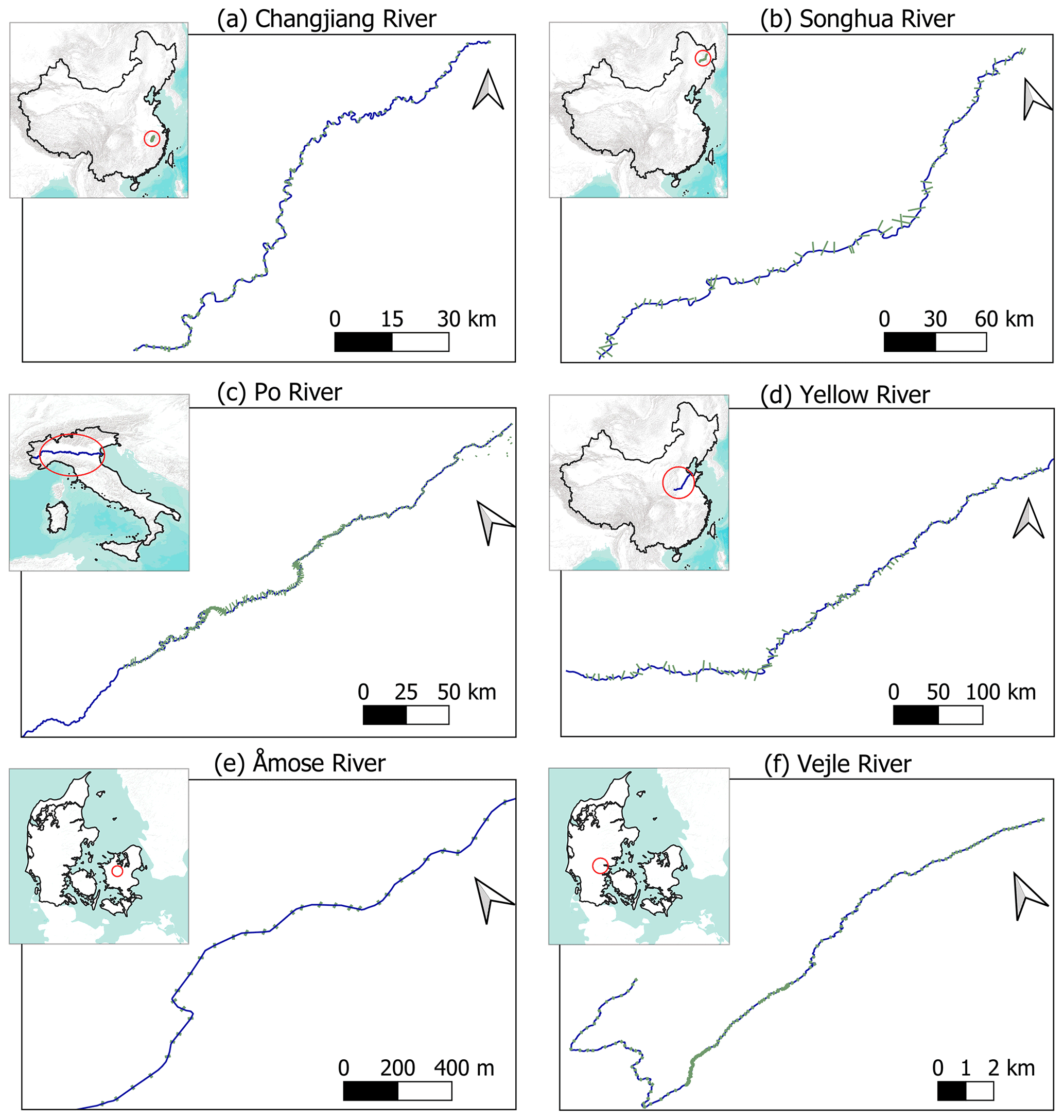
Figure A1Location and river setting of six rivers. Short grey lines indicate cross-sections used to explore the hydraulic relationships.
Further, we can write it as with and .
Therefore, α is linearly related to γ although the intercept (m) and slope (n) are not constant. That is, Eq. (A2) is valid at each individual cross-section.
Similarly, if we divide Eq. (6) by Eq. (7), we can obtain
When taking the logarithm and rearranging the equation, we have
Thus, β can also be expressed as a linear function of δ but with varying intercept.
One should not confuse Eqs. (A2) and (A4) with Eqs. (11) and (12). The first two equations are derived at individual cross-section, while the last two equations are derived by fitting linear functions to cross-section parameters at the reach scale.
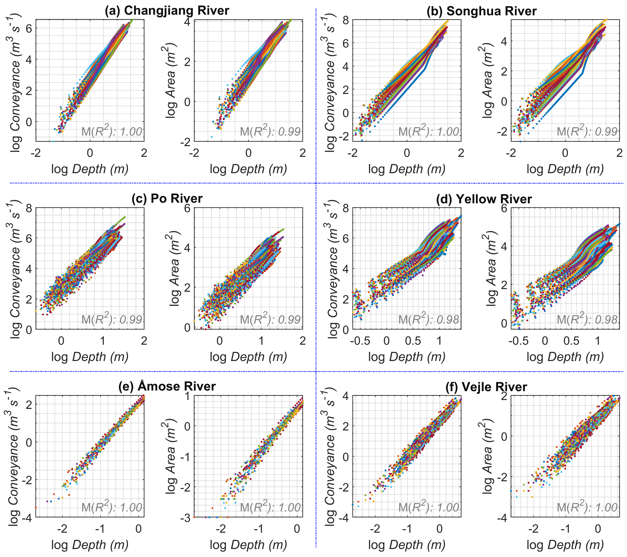
Figure A2Relationship between logarithmic depth and logarithmic area and logarithmic conveyance. Similar to Fig. 1 but a uniform Manning's coefficient of 0.03 was used to calculate conveyance. This results in a stronger linear relationship. However, a uniform Manning's coefficient is not very realistic in natural rivers.
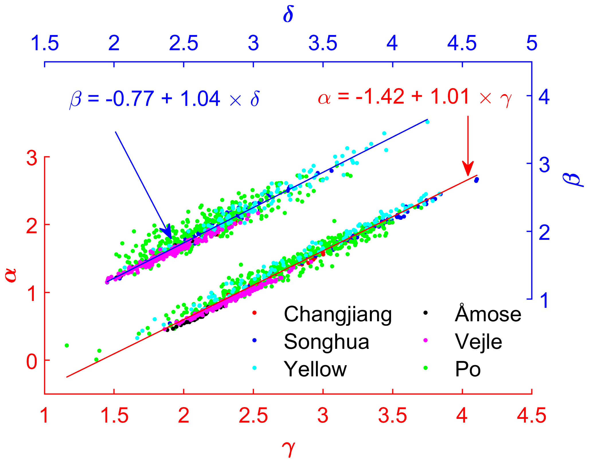
Figure A3Linear relationships between γ–α and δ–β using data of all six rivers. Similar to Fig. 2, but a uniform Manning's coefficient of 0.03 was used.
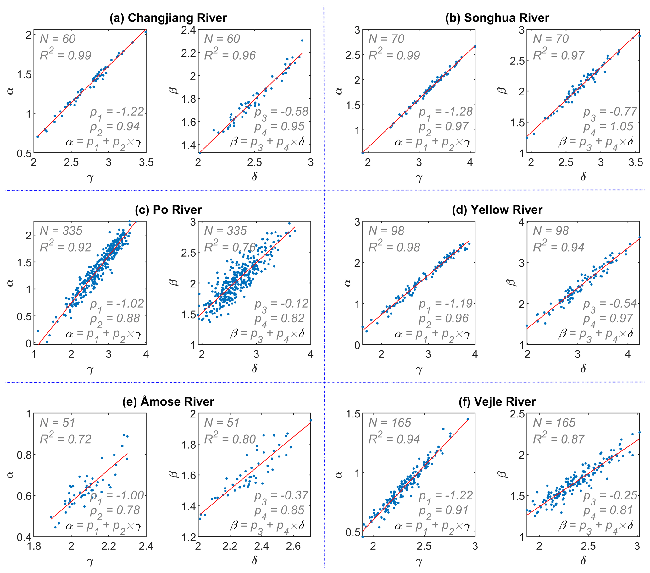
Figure A4Linear relationships between γ–α and δ–β for six rivers. Randomly generated Manning's coefficient in the range of 0.015–0.05 for each cross-section was used to calculate conveyance. The number of cross-sections, coefficient of determination, and regression coefficients are labeled in each plot.
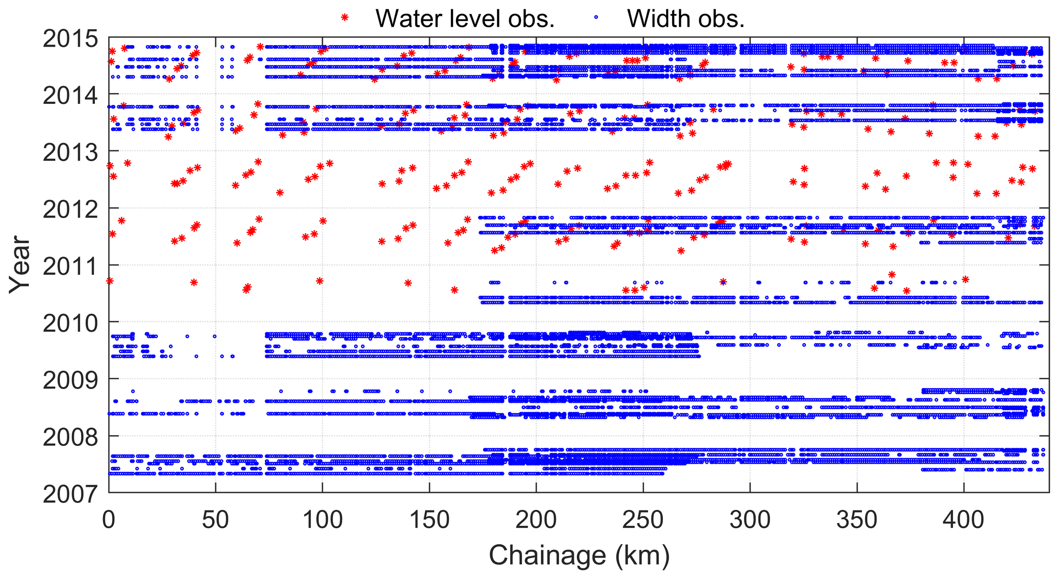
Figure B1Temporal and spatial distribution of water levels and widths, which are used to calibrate the model. Given that the river is frozen in cold season, only data in warm seasons are used. Landsat 5/8 images with low cloud cover (visual checked in Google Earth Engine) are selected to generate river width.
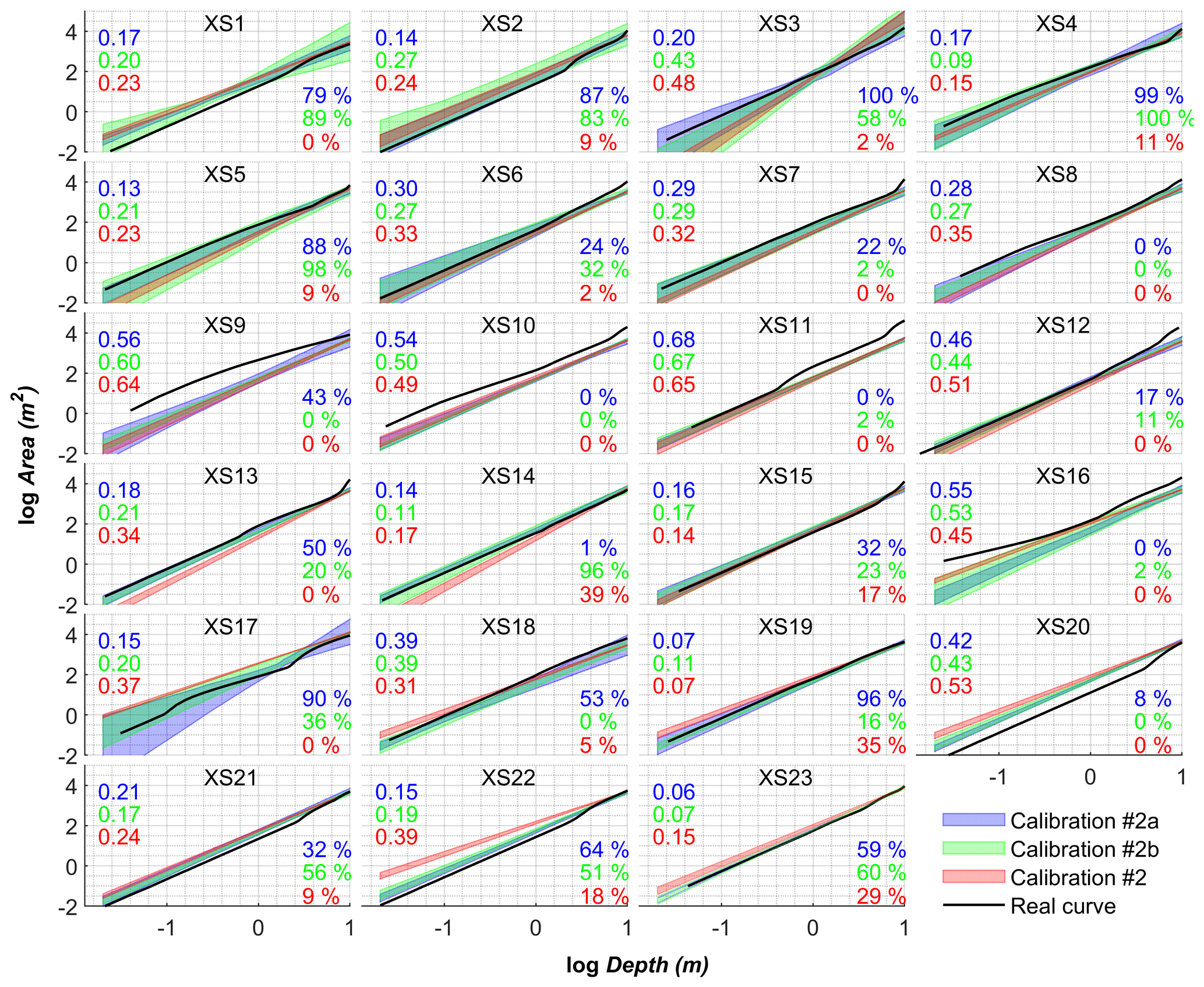
Figure B2Calibrated curves using three scenarios of width observations only, i.e., one width observation per 5 km reach (calibration #2a), one width observation per 2 km reach (calibration #2b), and all available widths (calibration #2). The color band represents the mean ± standard deviation based on an ensemble of 10 calibrations. The number of cross-section is given in each plot. RMSE and coverage of calibrated curves against real data are reported on the left and right sides of each plot, respectively. Font color is consistent with the curve color. The average RMSE and coverage values are 0.28, 0.30, and 0.34 and 45 %, 36 %, and 8 % for calibration #2a, #2b, and #2, respectively.
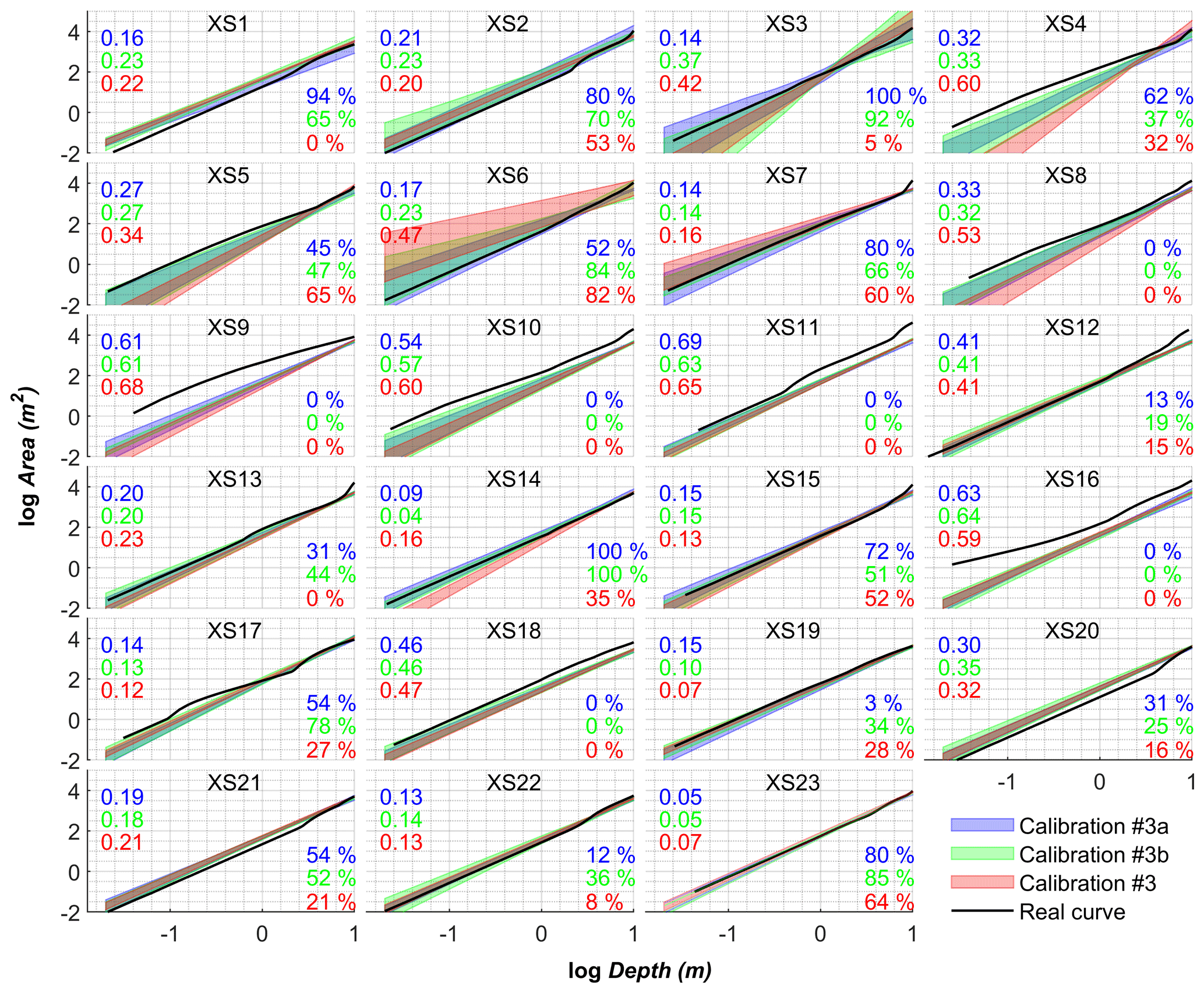
Figure B3Calibrated curves using three scenarios of width observations and water level, i.e., one width observation per 5 km reach and water levels (calibration #3a), one width observation per 2 km reach and water levels (calibration #3b), and all available widths and water levels (calibration #3). The color band represents the mean ± standard deviation based on an ensemble of 10 calibrations. The number of cross-section is given in each plot. RMSE and coverage (percentage of real data falling into the calibrated interval) of calibrated curves against real data are reported on the left and right sides of each plot, respectively. Font color is consistent with the curve color. The average RMSE and coverage values are 0.28, 0.29, and 0.34 and 41 %, 42 %, and 24 % for calibration #3a, #3b, and #3, respectively.
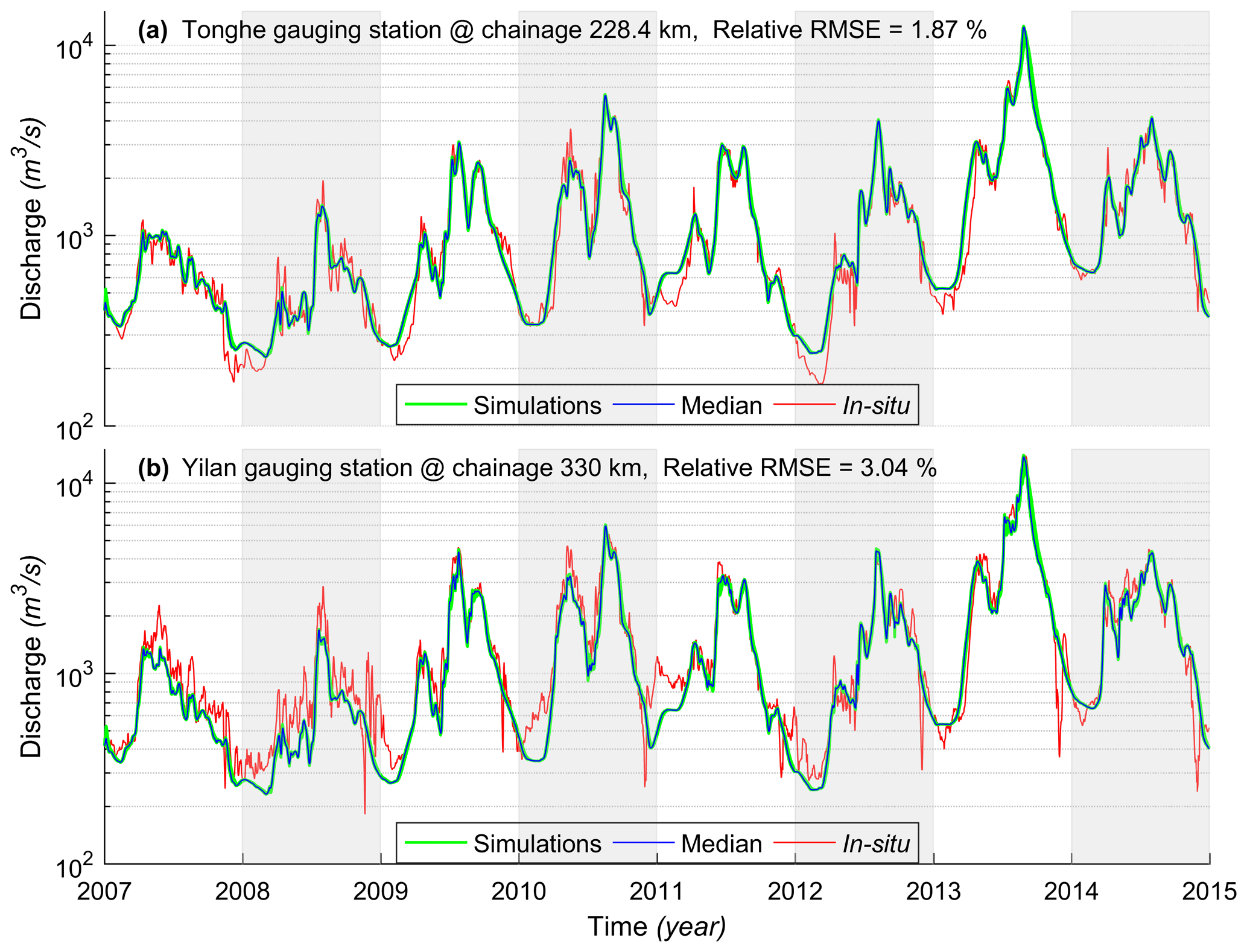
Figure C1Validation of simulated discharge at two gauging stations. Note, in each plot, results of the median and individual simulations of an ensemble of 30 calibrations (i.e., calibrations #1, #2, and #3) are shown.

Figure C2Comparison of model simulated water level, width, and datum using different calibration data sets. (a) Calibration #1; (b) calibration #2a; (c) calibration #2b; (d) calibration #2; (e) calibration #3a; (f) calibration #3b, and (g) calibration #3. Note that y axes are in log scale. Color bands indicate the boundary (i.e., maximum and minimum) of simulations. Along with model simulations, satellite observations of WSE and width are plotted.
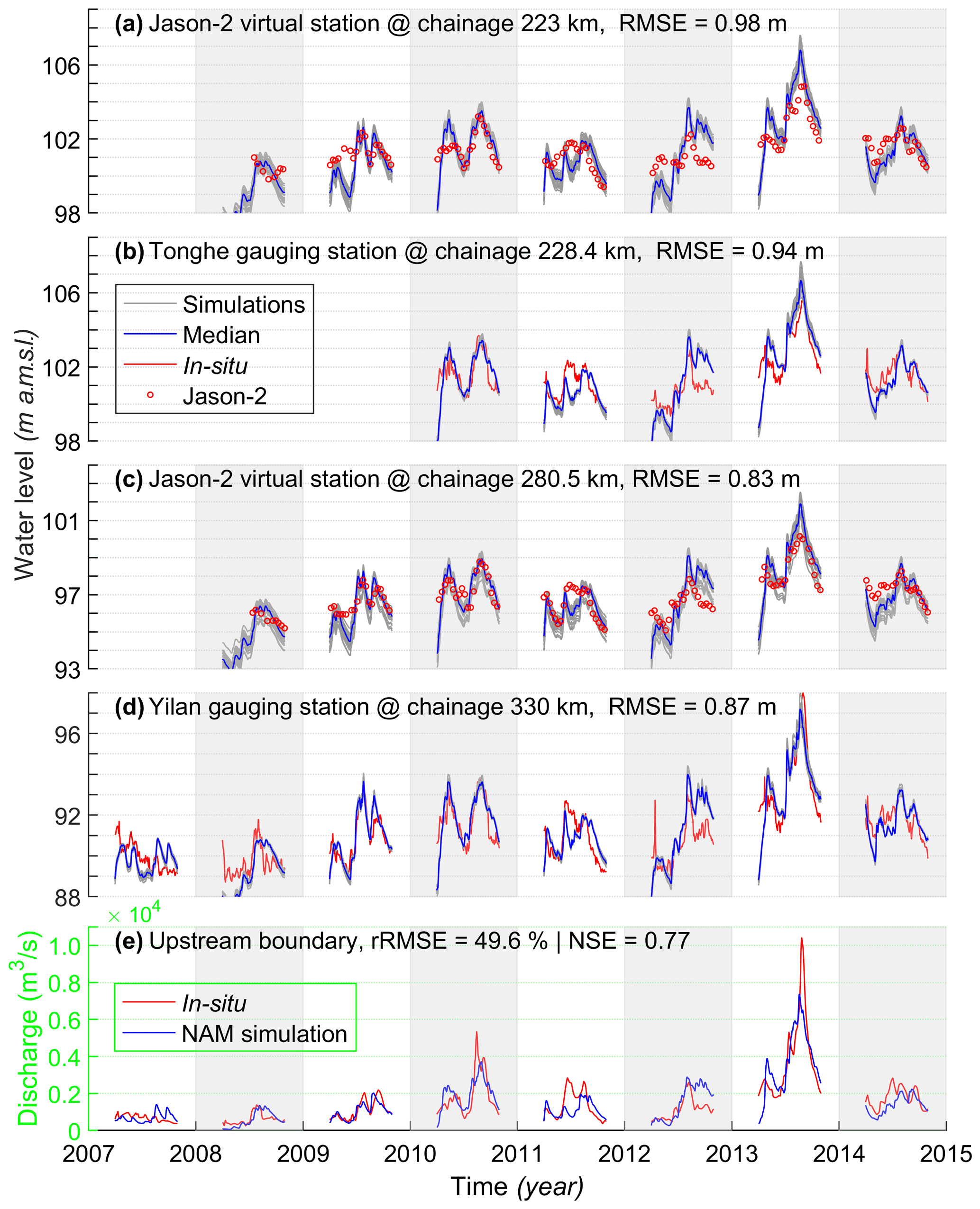
Figure C3Similar to Fig. 6 but upstream boundary is rainfall-runoff model simulation instead of in situ discharge, which are shown in panel (e). Note that NAM model was not calibrated at this location.
River widths were processed on the Google Earth Engine platform. CryoSat-2 were from the study of Jiang et al. (2019). Jason-2 data were downloaded from AVISO+ (https://www.aviso.altimetry.fr/en/data/data-access/ftp.html; AVISO+, 2021). Cross-section data of the Changjiang, Songhua, and Yellow rivers were excerptedfrom the Hydrological Yearbook 2007–2014 issued by the Ministry of Water Resources, China. Cross-section data of the Po river are publicly available from the Interregional agency for the river Po (http://geoportale.agenziapo.it/web/index.php/it/?option=com_aipografd3; AIPo, 2021). Data of the Danish rivers (Åmose, Vejle) were kindly provided by WSP (http://www.hydrometri.dk/hyd/; HYDROMETRI.DK, 2021). The main MATLAB scripts are publicly available on Zenodo (https://doi.org/10.5281/zenodo.5782990; Jiang et al., 2021).
SWC developed the methodology in an early stage with inputs from LJ and PBG. LJ further developed the methodology, did the data curation, and performed the calibration work. LJ prepared the article. All authors contributed to editing the article.
The contact author has declared that neither they nor their co-authors have any competing interests.
Publisher's note: Copernicus Publications remains neutral with regard to jurisdictional claims in published maps and institutional affiliations.
The authors would like to thank AVISO+, WSP, and AIPo for making the data sets available.
This work was jointly funded by the Danida Fellowship Centre (EOForChina project, file number: 18-M01-DTU) and the Innovation Fund Denmark (ChinaWaterSense project, file number: 8087-00002B).
This paper was edited by Albrecht Weerts and reviewed by Guy J.-P. Schumann, Dai Yamazaki and Karl Kästner.
AIPo: http://geoportale.agenziapo.it/web/index.php/it/?option=com_aipografd3, last access: 15 December 2021.
Andreadis, K. M. and Schumann, G. J. P.: Estimating the impact of satellite observations on the predictability of large-scale hydraulic models, Adv. Water Resour., 73, 44–54, https://doi.org/10.1016/j.advwatres.2014.06.006, 2014.
Annis, A., Nardi, F., Volpi, E., and Fiori, A.: Quantifying the relative impact of hydrological and hydraulic modelling parameterizations on uncertainty of inundation maps, Hydrolog. Sci. J., 65, 507–523, https://doi.org/10.1080/02626667.2019.1709640, 2020.
Aster, R. C., Borchers, B., and Thurber, C. H.: Parameter estimation and inverse problems, Elsevier, Amsterdam, the Netherlands, 2018.
AVISO+: FTP, available at: https://www.aviso.altimetry.fr/en/data/data-access/ftp.html, last access: 15 December 2021.
Bandini, F., Sunding, T. P., Linde, J., Smith, O., Jensen, I. K., Köppl, C. J., Butts, M., and Bauer-Gottwein, P.: Unmanned Aerial System (UAS) observations of water surface elevation in a small stream: Comparison of radar altimetry, LIDAR and photogrammetry techniques, Remote Sens. Environ., 237, 111487, https://doi.org/10.1016/j.rse.2019.111487, 2020.
Bates, P. D., Neal, J. C., Alsdorf, D., and Schumann, G. J.-P.: Observing Global Surface Water Flood Dynamics, Surv. Geophys., 35, 839–852, https://doi.org/10.1007/s10712-013-9269-4, 2014.
Biancamaria, S., Lettenmaier, D. P., and Pavelsky, T. M.: The SWOT Mission and Its Capabilities for Land Hydrology, Surv. Geophys., 37, 307–337, https://doi.org/10.1007/s10712-015-9346-y, 2016.
Bierkens, M. F. P.: Global hydrology 2015: State, trends, and directions, Water Resour. Res., 51, 4923–4947, https://doi.org/10.1002/2015WR017173, 2015.
Bjerklie, D. M., Moller, D., Smith, L. C., and Dingman, S. L.: Estimating discharge in rivers using remotely sensed hydraulic information, J. Hydrol., 309, 191–209, https://doi.org/10.1016/j.jhydrol.2004.11.022, 2005.
Blöschl, G., Gaál, L., Hall, J., Kiss, A., Komma, J., Nester, T., Parajka, J., Perdigão, R. A. P., Plavcová, L., Rogger, M., Salinas, J. L., and Viglione, A.: Increasing river floods: fiction or reality?, Wiley Interdisciplin. Rev. Water, 2, 329–344, https://doi.org/10.1002/wat2.1079, 2015.
Brisset, P., Monnier, J., Garambois, P.-A., and Roux, H.: On the assimilation of altimetric data in 1D Saint–Venant river flow models, Adv. Water Resour., 119, 41–59, https://doi.org/10.1016/j.advwatres.2018.06.004, 2018.
Broyden, C. G.: A class of methods for solving nonlinear simultaneous equations, Math. Comput., 19, 577–577, https://doi.org/10.1090/S0025-5718-1965-0198670-6, 1965.
Chow, V. Te: Open channel hydraulics, McGraw-Hill Book Company, Inc, New York, 1959.
Dey, S., Saksena, S., and Merwade, V.: Assessing the effect of different bathymetric models on hydraulic simulation of rivers in data sparse regions, J. Hydrol., 575, 838–851, https://doi.org/10.1016/j.jhydrol.2019.05.085, 2019.
DHI: MIKE HYDRO River – User Guide, DHI, Copenhagen, 2017.
Dingman, S. L.: Analytical derivation of at-a-station hydraulic–geometry relations, J. Hydrol., 334, 17–27, https://doi.org/10.1016/j.jhydrol.2006.09.021, 2007.
Domeneghetti, A.: On the use of SRTM and altimetry data for flood modeling in data-sparse regions, Water Resour. Res., 52, 2901–2918, https://doi.org/10.1002/2015WR017967, 2016.
Domeneghetti, A., Tarpanelli, A., Brocca, L., Barbetta, S., Moramarco, T., Castellarin, A., and Brath, A.: The use of remote sensing-derived water surface data for hydraulic model calibration, Remote Sens. Environ., 149, 130–141, https://doi.org/10.1016/j.rse.2014.04.007, 2014.
Durand, M., Andreadis, K. M., Alsdorf, D. E., Lettenmaier, D. P., Moller, D., and Wilson, M.: Estimation of bathymetric depth and slope from data assimilation of swath altimetry into a hydrodynamic model, Geophys. Res. Lett., 35, L20401, https://doi.org/10.1029/2008GL034150, 2008.
Ferguson, R. I.: Hydraulics and hydraulic geometry, Prog. Phys. Geogr. Earth Environ., 10, 1–31, https://doi.org/10.1177/030913338601000101, 1986.
Fleischmann, A., Paiva, R., and Collischonn, W.: Can regional to continental river hydrodynamic models be locally relevant? A cross-scale comparison, J. Hydrol., 3, 100027, https://doi.org/10.1016/j.hydroa.2019.100027, 2019.
Fonstad, M. A. and Marcus, W. A.: Remote sensing of stream depths with hydraulically assisted bathymetry (HAB) models, Geomorphology, 72, 320–339, https://doi.org/10.1016/j.geomorph.2005.06.005, 2005.
Garambois, P. A. and Monnier, J.: Inference of effective river properties from remotely sensed observations of water surface, Adv. Water Resour., 79, 103–120, https://doi.org/10.1016/j.advwatres.2015.02.007, 2015.
Garambois, P.-A., Calmant, S., Roux, H., Paris, A., Monnier, J., Finaud-Guyot, P., Samine Montazem, A., and Santos da Silva, J.: Hydraulic visibility: Using satellite altimetry to parameterize a hydraulic model of an ungauged reach of a braided river, Hydrol. Process., 31, 756–767, https://doi.org/10.1002/hyp.11033, 2017.
Garbrecht, J.: Analytical representation of cross-section hydraulic properties, J. Hydrol., 119, 43–56, https://doi.org/10.1016/0022-1694(90)90033-T, 1990.
Gleason, C. J.: Hydraulic geometry of natural rivers: A review and future directions, Prog. Phys. Geogr., 39, 337–360, https://doi.org/10.1177/0309133314567584, 2015.
Gleason, C. J. and Durand, M. T.: Remote Sensing of River Discharge: A Review and a Framing for the Discipline, Remote Sens., 12, 1107, https://doi.org/10.3390/rs12071107, 2020.
Grimaldi, S., Li, Y., Walker, J. P., and Pauwels, V. R. N.: Effective Representation of River Geometry in Hydraulic Flood Forecast Models, Water Resour. Res., 54, 1031–1057, https://doi.org/10.1002/2017WR021765, 2018.
HYDROMETRI.DK: Vandløbssiden, available at: http://www.hydrometri.dk/hyd/, last access: 15 December 2021.
Jiang, L., Nielsen, K., Andersen, O. B., and Bauer-Gottwein, P.: CryoSat-2 radar altimetry for monitoring freshwater resources of China, Remote Sens. Environ., 200, 125–139, https://doi.org/10.1016/j.rse.2017.08.015, 2017.
Jiang, L., Madsen, H., and Bauer-Gottwein, P.: Simultaneous calibration of multiple hydrodynamic model parameters using satellite altimetry observations of water surface elevation in the Songhua River, Remote Sens. Environ., 225, 229–247, https://doi.org/10.1016/j.rse.2019.03.014, 2019.
Jiang, L., Bandini, F., Smith, O., Klint Jensen, I., and Bauer-Gottwein, P.: The Value of Distributed High-Resolution UAV-Borne Observations of Water Surface Elevation for River Management and Hydrodynamic Modeling, Remote Sens., 12, 1171, https://doi.org/10.3390/rs12071171, 2020.
Jiang, L., Christensen, S. W., and Bauer-Gottwein, P.: Calibrating 1D hydrodynamic river models in the absence of cross-section geometry in DHI MIKE HYDRO, Zenodo [code], https://doi.org/10.5281/zenodo.5782990, 2021.
Larnier, K., Monnier, J., Garambois, P. A., and Verley, J.: River discharge and bathymetry estimation from SWOT altimetry measurements, Inverse Probl. Sci. Eng., 29, 759–789, https://doi.org/10.1080/17415977.2020.1803858, 2021.
Legleiter, C. J.: Calibrating remotely sensed river bathymetry in the absence of field measurements: Flow REsistance Equation-Based Imaging of River Depths (FREEBIRD), Water Resour. Res., 51, 2865–2884, https://doi.org/10.1002/2014WR016624, 2015.
Leopold, L. B. and Maddock, T. J.: The Hydraulic Geometry of Stream Channels and Some Physiographic Implications, Geol. Surv. Prof. Pap. 252, United States Government Printing Office, Washington, 1–57, 1953.
Liu, G., Schwartz, F. W., Tseng, K.-H., and Shum, C. K.: Discharge and water-depth estimates for ungauged rivers: Combining hydrologic, hydraulic, and inverse modeling with stage and water-area measurements from satellites, Water Resour. Res., 51, 6017–6035, https://doi.org/10.1002/2015WR016971, 2015.
Madsen, K., Nielsen, H. B., and Tingleff, O.: Methods for Non-Linear Least Squares Problems, in: Lecture note, Informatics and Mathematical Modelling, 2nd Edn., Technical University of Denmark, 2004.
Marquardt, D. W.: An Algorithm for Least-Squares Estimation of Nonlinear Parameters, J. Soc. Ind. Appl. Math., 11, 431–441, https://doi.org/10.1137/0111030, 1963.
Mejia, A. I. and Reed, S. M.: Evaluating the effects of parameterized cross-section shapes and simplified routing with a coupled distributed hydrologic and hydraulic model, J. Hydrol., 409, 512–524, https://doi.org/10.1016/j.jhydrol.2011.08.050, 2011.
Mersel, M. K., Smith, L. C., Andreadis, K. M., and Durand, M. T.: Estimation of river depth from remotely sensed hydraulic relationships, Water Resour. Res., 49, 3165–3179, https://doi.org/10.1002/wrcr.20176, 2013.
Michailovsky, C. I., McEnnis, S., Berry, P. A. M., Smith, R., and Bauer-Gottwein, P.: River monitoring from satellite radar altimetry in the Zambezi River basin, Hydrol. Earth Syst. Sci., 16, 2181–2192, https://doi.org/10.5194/hess-16-2181-2012, 2012.
Milzow, C., Krogh, P. E., and Bauer-Gottwein, P.: Combining satellite radar altimetry, SAR surface soil moisture and GRACE total storage changes for hydrological model calibration in a large poorly gauged catchment, Hydrol. Earth Syst. Sci., 15, 1729–1743, https://doi.org/10.5194/hess-15-1729-2011, 2011.
Moramarco, T., Barbetta, S., Bjerklie, D. M., Fulton, J. W., and Tarpanelli, A.: River Bathymetry Estimate and Discharge Assessment from Remote Sensing, Water Resour. Res., 55, 6692–6711, https://doi.org/10.1029/2018WR024220, 2019.
Neal, J., Schumann, G., and Bates, P.: A subgrid channel model for simulating river hydraulics and floodplain inundation over large and data sparse areas, Water Resour. Res., 48, 1–16, https://doi.org/10.1029/2012WR012514, 2012.
Neal, J. C., Odoni, N. A., Trigg, M. A., Freer, J. E., Garcia-pintado, J., Mason, D. C., Wood, M., and Bates, P. D.: Efficient incorporation of channel cross-section geometry uncertainty into regional and global scale flood inundation models, J. Hydrol., 529, 169–183, https://doi.org/10.1016/j.jhydrol.2015.07.026, 2015.
Nielsen, H. B. and Völcker, C.: IMMOPTIBOX: A Matlab Toolbox for Optimization and Data Fitting, available at: http://www2.imm.dtu.dk/projects/immoptibox/ (last access: 15 December 2021), 2010.
Pappenberger, F., Beven, K., Frodsham, K., Romanowicz, R., and Matgen, P.: Grasping the unavoidable subjectivity in calibration of flood inundation models: A vulnerability weighted approach, J. Hydrol., 333, 275–287, https://doi.org/10.1016/j.jhydrol.2006.08.017, 2007.
Pereverzyev, S. S., Pinnau, R., and Siedow, N.: Regularized fixed-point iterations for non-linear inverse problems, Inverse Probl., 22, 1–22, https://doi.org/10.1088/0266-5611/22/1/001, 2006.
Schaperow, J. R., Li, D., Margulis, S. A., and Lettenmaier, D. P.: A Curve-Fitting Method for Estimating Bathymetry From Water Surface Height and Width, Water Resour. Res., 55, 4288–4303, https://doi.org/10.1029/2019WR024938, 2019.
Schmidt, M.: Least Squares Optimization with L1-Norm Regularization, Proj. Rep. 98, 230–238, available at: https://www.cs.ubc.ca/~schmidtm/Software/lasso.html (last access: 15 December 2021), 2005.
Schneider, R., Godiksen, P. N., Villadsen, H., Madsen, H., and Bauer-Gottwein, P.: Application of CryoSat-2 altimetry data for river analysis and modelling, Hydrol. Earth Syst. Sci., 21, 751–764, https://doi.org/10.5194/hess-21-751-2017, 2017.
Schneider, R., Ridler, M. E., Godiksen, P. N., Madsen, H., and Bauer-Gottwein, P.: A data assimilation system combining CryoSat-2 data and hydrodynamic river models, J. Hydrol., 557, 197–210, https://doi.org/10.1016/j.jhydrol.2017.11.052, 2018.
Schumann, G., Matgen, P., Hoffmann, L., Hostache, R., Pappenberger, F., and Pfister, L.: Deriving distributed roughness values from satellite radar data for flood inundation modelling, J. Hydrol., 344, 96–111, https://doi.org/10.1016/j.jhydrol.2007.06.024, 2007.
Songliao River Conservancy Commission: The Songhua River, Changchun, China, 2004.
Songliao River Conservancy Commission: Water resources bulletin of Songhua & Liao River, Changchun, China, available at: http://www.slwr.gov.cn/ (last access: 15 December 2021), 2015.
Sun, W. C., Ishidaira, H., and Bastola, S.: Towards improving river discharge estimation in ungauged basins: Calibration of rainfall-runoff models based on satellite observations of river flow width at basin outlet, Hydrol. Earth Syst. Sci., 14, 2011–2022, https://doi.org/10.5194/hess-14-2011-2010, 2010.
Ward, P. J., Jongman, B., Salamon, P., Simpson, A., Bates, P., De Groeve, T., Muis, S., de Perez, E. C., Rudari, R., Trigg, M. A., and Winsemius, H. C.: Usefulness and limitations of global flood risk models, Nat. Clim. Change, 5, 712–715, https://doi.org/10.1038/nclimate2742, 2015.
Yamazaki, D., Kanae, S., Kim, H., and Oki, T.: A physically based description of floodplain inundation dynamics in a global river routing model, Water Resour. Res., 47, W04501, https://doi.org/10.1029/2010WR009726, 2011.
Yang, X., Pavelsky, T. M., Allen, G. H., and Donchyts, G.: RivWidthCloud: An Automated Google Earth Engine Algorithm for River Width Extraction From Remotely Sensed Imagery, IEEE Geosci. Remote Sens. Lett., 17, 217–221, https://doi.org/10.1109/LGRS.2019.2920225, 2020.
- Abstract
- Introduction
- Methods
- Case study
- Results
- Discussion
- Conclusions
- Appendix A: Supplementary information on the relationships between flow-area/conveyance and depth
- Appendix B: Supplementary information on the data sets and calibrated curves
- Appendix C: Supplementary information on the simulation results
- Code and data availability
- Author contributions
- Competing interests
- Disclaimer
- Acknowledgements
- Financial support
- Review statement
- References