Comment on: “A review of the complementary principle of evaporation: from the original linear relationship to generalized nonlinear functions” by Han and Tian (2020)

The paper by Han and Tian (2020) reviews the history of developments in the complementary relationship (CR) between actual and potential evaporation and introduces the generalized complementary principle (GCP) developed by the authors. This comment assesses whether the GCP: (1) can give reasonable results from a wide range of surfaces worldwide; (2) is supported by experimental data that verify the three stages of evaporation implicit in the GCP, particularly in the wet-surface limit; (3) has been proven to be correct by the authors in a previous paper; and (4) is supported by model studies showing that wet surfaces occur predominantly during periods of large-scale moisture convergence. The assessment finds that arguments in favor of the GCP deserve to be taken seriously but ultimately remain unconvincing.

1 Introduction

Han and Tian (2020) (hereafter HT20) provide important insights into the growing body of literature regarding the complementary relationship (CR) of evaporation and serves well as an accessible review of the literature. The sigmoid formulation (their Eq. 13), a key feature of their generalized complementary principle (GCP) (Han and Tian, 2018; hereafter HT18), is presented and defended in their paper.

Two of the present authors (Szilagyi and Crago, 2019, hereafter SC19) wrote an earlier comment critiquing the sigmoid function for violating established physical principles (see also the reply by Han and Tian, 2019). After further consideration, the present authors recognize that the sigmoid curve proposed by HT18 and HT20 is intended to incorporate the effects of both the CR and of large-scale advection under wet-surface conditions. While we do not find the sigmoid function to have a strong theoretical or empirical basis, we agree with HT18 and HT20, at least in principle, that this need not violate any laws of nature. (Note that, unless otherwise indicated, all notation herein follows that of HT20.)

The most controversial feature of the sigmoid function is the slope of the curve at the wet-surface limit. Namely, it requires that $\mathrm{d}(E/E_{\mathrm{Pen}})/\mathrm{d}(E_{\mathrm{rad}}/E_{\mathrm{Pen}})=\mathrm{d}{y}_{\mathrm{H}}/\mathrm{d}{x}_{\mathrm{H}}\to \mathrm{0}$ as y_H→1 (hereafter, this boundary condition will be denoted “BC4”). That is, rather than a complementary relationship, BC4 requires that E and E_Pen are equal and that E exactly follows any variability by E_Pen in the wet-surface limit.

BC4 deserves careful attention. A major purpose of this comment is to show that there are some indications that such behavior can occur, but when it does it is a consequence of large-scale processes that disconnect the regional land surface from the overlying atmosphere, thus violating the basic assumptions behind the CR (namely, that atmospheric and surface conditions are tightly linked through surface fluxes). In light of this, corrections to the CR attempting to account for these cases will likely result in a formulation that does not accurately represent minimally advective conditions.

This comment will consider the evidence for the following four claims made by HT18 and HT20 in support of the sigmoid function and BC4: first, that the function works reasonably well to model evaporation from sites around the world; second, that data from these sites support a three-stage evaporation process and BC4, both of which are required by the sigmoid function; third, that HT2018 have provided a rigorous proof of the boundary conditions underlying the formulation; and fourth, that a partial explanation of BC4 has been provided by the study by Lintner et al. (2015).

2 Claim regarding modeling results

First, it is clear that the sigmoid function has been used successfully to model evaporation from flux stations around the world (see HT18). It is quite a flexible formulation that can match a wide range of data patterns on an x_H, y_H graph. Calibrated values of α and b published in HT18 (their Table 5) range from about 1.01 to 1.49 and from 0.59 to 17, respectively. Figure 1 shows the sigmoid function for the four combinations of these extreme parameter values (with $x_{min}=\mathrm{0}$ and $x_{max}=\mathrm{1}$). These show the wide range of possible curve shapes, allowing x_min and x_max to take other fixed values further increases the flexibility. Such an equation is likely to fit many datasets well if tuning is permitted. While we believe the ultimate goal of CR research should be a physically based formulation that can work well without requiring local calibration of parameters, there is, nevertheless, value in formulations that can reliably match datasets with local calibration (including several of our respective publications).

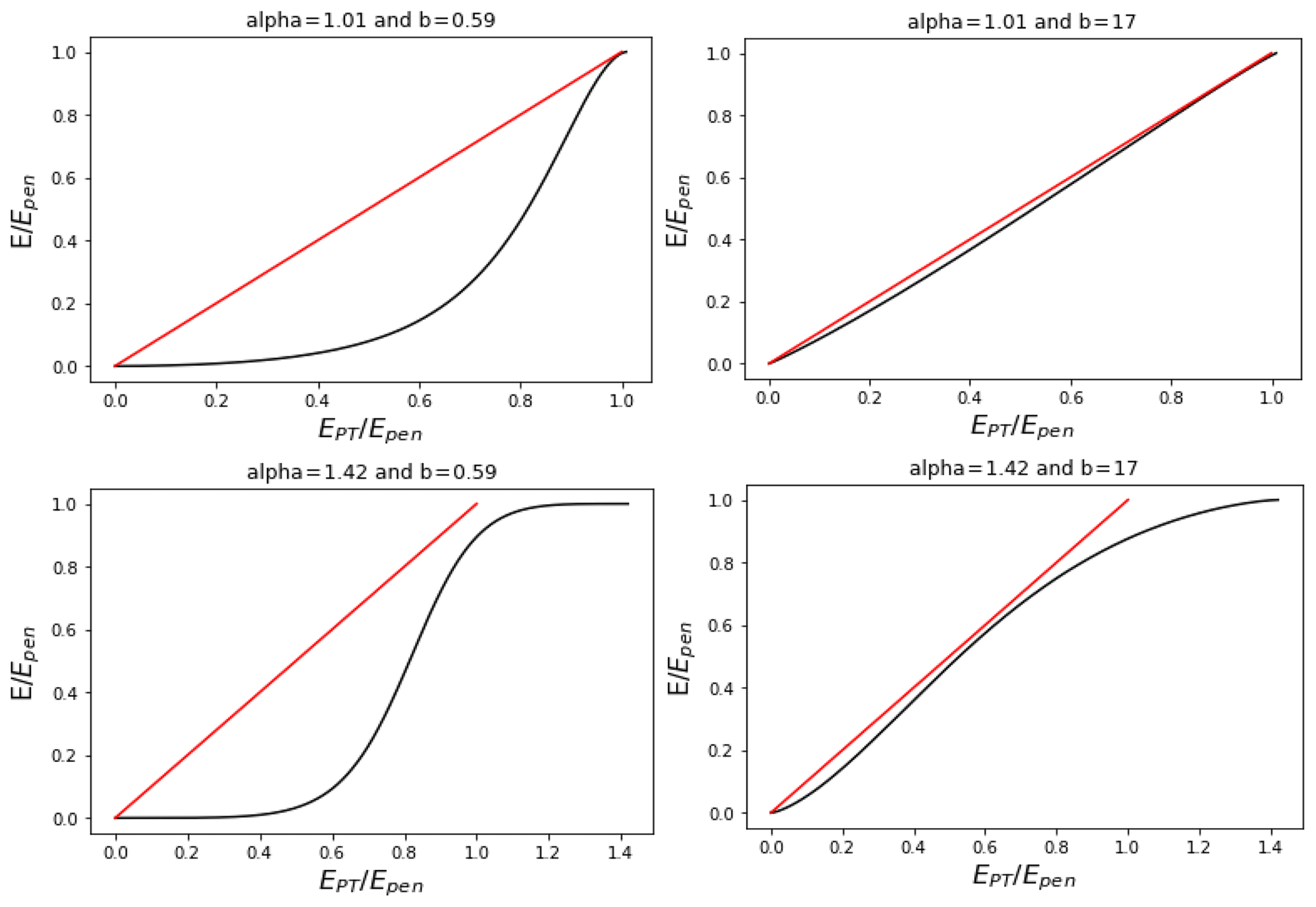
Figure 1 The sigmoid function (black curves) and the Priestley–Taylor line (α=1.26, straight line in red) for the most extreme parameter values documented in HT18. The scales of the horizontal axes differ.

3 Claim regarding empirical support for three evaporation stages and for BC4

Second, there does seem to be some empirical support for different slopes at different positions on x_H, y_H graphs (HT18, their Table 3). However, the curve proposed by Brutsaert (2015) also proposes a shallow slope for small y_H (stage 1), a steep slope in the middle (stage 2), and a less steep slope near y_H=1 (stage 3). Similar behavior is also possible with the rescaled models of the present authors. The stage 3 slopes at large y_H values (HT18, Table 3) would be near zero according to BC4 but are generally near 1 instead. HT18 directly address BC4 with data in their Fig. 6, which plots empirical data along with red curves resulting from the sigmoid function relating E∕E_PT to E∕E_Pen. The sigmoid function curves show E∕E_PT increasing as E∕E_Pen increases, until E∕E_PT reaches a peak and then begins to decrease with further increases in E∕E_Pen. Correlational evidence for this downturn is given by HT18, but the actual data plotted do not visibly follow the downturn in E∕E_PT in either panel of Fig. 6; the dramatic downturn in the red curve in Fig. 6a (the left panel) certainly is not matched by the data. While the limiting behavior would only be expected very near y_H=1, this very fact makes it difficult to argue that this behavior exists when nearly all data points on the graph fall below y_H=1. Similarly, some values of parameters for the sigmoid function make the flattening of the third stage nearly indistinguishable and therefore inconsequential (i.e., the top two panels of our Fig. 1).

4 Claim regarding the derivation by HT18

Third, the derivation by HT18 is inconclusive. The derivation begins with the following (HT18, their Eq. 8):

$$\begin{array}{}\text{(1)}& E=\left(E_{\mathrm{Pen}}\right)\cdot f(E_{\mathrm{rad}}/E_{\mathrm{Pen}}),\text{where}{E}_{\mathrm{Pen}}=E_{\mathrm{rad}}+E_{\mathrm{aero}},\end{array}$$

where f is a function of E_rad∕E_Pen. Partial derivatives of E were taken from Eq. (1) with respect to E_rad and E_aero. Further manipulations of these derivatives resulted in the four boundary conditions corresponding to the sigmoid curve (HT18). The function f(E_rad∕E_Pen) in Eq. (1) could include constants or parameters (for instance α, x_min, or x_max), whose “correct” values can be found by calibration, after which they must be treated as constants. This means that, once the parameters are determined, the shape of f(E_rad∕E_Pen) is also determined.

Unfortunately, this leads to two problems. First, the present authors' work with the “rescaled” CR (Crago et al., 2016; Szilagyi et al., 2017; Crago and Qualls, 2018) gives evidence that the variable $x_{\mathrm{m}}={E^{T_{\mathrm{ws}}}}_{\mathrm{PT}}/{E^{max}}_{\mathrm{MT}}$ (where x_m is our own notation), related to the value of ${E^{T_{\mathrm{ws}}}}_{\mathrm{PT}}/E_{\mathrm{Pen}}$ at which E goes to zero, is in fact a variable not a constant. It must be calculated for each individual data point, and it results in a significant rearrangement of the data. It could have been included in Eq. (1) by writing Eq. (1) as y_H=f(x_H, x_m). By taking derivatives without including the impact that a variable x_m might have, HT18 assumed from the beginning that E∕E_Pen does not vary with x_m, so a variable x_m boundary condition could not possibly arise from this derivation. On the other hand, if x_m is in fact a significant variable (as the papers cited above suggest), it could impact the entire derivation but particularly the two dry-limit boundary conditions.

The parameter x_max is the maximum value x_H can reach and is usually taken by HT18 and HT20 to be 1.26⁻¹, where 1.26 is the commonly accepted value for the Priestley and Taylor parameter α. To prove that $\mathrm{d}{y}_{\mathrm{H}}/\mathrm{d}{x}_{\mathrm{H}}\to \mathrm{0}$ as y_H→1 (the most controversial finding of the derivation), HT18 had to show that $\partial x_{max}/\partial E_{\mathrm{rad}}$ evaluated at y=1 cannot be 0 (see the paragraph starting at the bottom of page 5054 and ending at the top of page 5055 of HT18). But if Eq. (1) is true, x_max has to be treated as a constant, so the partial derivative must be 0. It is impossible for x_max to be a constant for the purpose of taking derivatives of Eq. (1) but a variable when evaluating $\partial x_{max}/\partial E_{\mathrm{rad}}$. Thus, there is a logical inconsistency hidden in this derivation. SC19 showed that, if the Priestley–Taylor α (equivalent here to $\mathrm{1}/x_{max}$) is actually a constant, the derivation by HT18 does not result in a specific required value for dy_H∕dx_H at y=1. Thus, the boundary condition $\mathrm{d}{y}_{\mathrm{H}}/\mathrm{d}{x}_{\mathrm{H}}\to \mathrm{0}$ as y_H→1 does not follow from Eq. (1).

To sum up consideration of the derivation, three of the four boundary conditions (slope and intercept at the point where y_H→0, and slope as y_H→1) are doubtful due to the assumptions made when Eq. (1) was used as the definition of E.

5 Claim regarding support from the modeling study by Lintner (2015)

HT18 cite the modeling results by Lintner et al. (2015) in support of BC4. This study used a steady-state model that captured the key physical processes affecting evaporation. Model results show decreases in both E_Pen and E as soil moisture approaches saturation, similar to the behavior required by BC4. According to Lintner et al. (2015; see also HT18), large-scale horizontal moisture convergence decreases E_Pen by increasing atmospheric humidity, and at the same time it increases precipitation and thus soil moisture content. Near the wet limit, water availability matters less than E_Pen in determining E, so E and E_Pen decrease at the same rate. Thus, at the point of saturation, E=E_Pen, and d($E/E_{\mathrm{Pen}})/\mathrm{d}(E_{\mathrm{PT}}/E_{\mathrm{Pen}})=\mathrm{0}$, apparently satisfying BC4.

CR researchers have long held that $E=E_{\mathrm{Pen}}=E_{\mathrm{PT}}$ for a wet regional surface (e.g., Brutsaert, 1982, 2005, 2015). The only way to get BC4-type behavior is to impose a large-scale process that causes E_Pen to differ from this value. That is, BC4 is not describing the drying process and the CR at all; rather, it is describing what happens when large-scale processes cause the CR to break down. The scenario described by Lintner et al. (2015) requires a clear disconnect between the land surface processes and the overlying atmospheric conditions, violating the central assumption of the CR (e.g., Brutsaert, 1982, 2005).

It need not be the case that nearly saturated surfaces coincide with moisture convergence in the real world. Nearly saturated surface conditions can exist under a range of large-scale patterns, including positive, negative, or negligible moisture convergence or advection. This is the case because soil moisture content varies at larger timescales than most other components of the surface water and energy budgets (e.g., Sellers et al., 1992), so nearly saturated surface conditions can persist after a period of moisture convergence has ended. Furthermore, saturated surfaces can occur from other processes, such as thunderstorms driven by surface heating.

A formulation that can account for varying advection would be desirable, and such methods have been previously proposed (e.g., Parlange and Katul, 1992). As already discussed, evidence that the sigmoid curve does this successfully is lacking. Furthermore, it seems to address advective effects only for wet surfaces, while advection clearly affects drying surfaces as well.

6 Conclusions

HT18 and HT20 have marshaled several empirical and theoretical arguments in support of their proposed sigmoid formulation of the CR. The range of arguments and data sources used is impressive, and the present authors only recently recognized the specific nature and the impact of this challenge on other CR formulations. There is little doubt that some aspects of their argument are true, including the ability of their formulation to match numerous experimental datasets. Nevertheless, the specific boundary conditions leading to the sigmoid function are not well-supported by empirical data; the derivation of the boundary conditions by HT18 was inconsistent regarding which model values are constants and which are variables; and the argument that large-scale processes require adoption of BC4 fails, because it implies that a disconnect between the land surface and the near-surface atmospheric conditions is the norm under near-wet-surface conditions, thus changing the shape of the CR with no solid theoretical or empirical arguments that it is in fact the norm. Attempts to adjust for other conditions (e.g., Parlange and Katul, 1992) are possible but should not override consideration of the basic CR concept. This may require developing specific conditions for screening data.

There does not seem to be consensus in the research community on any of the boundary conditions of the CR except for x_H=1 when y_H=1. The current authors find the evidence for a variable x_m to be strong. This value can be calculated separately for each data point, and it leads to a rescaling of the x_H axis and a resulting reduction in the scatter of the data points (Crago and Qualls, 2018).

While the sigmoid formulation is clearly the result of a serious and substantial research program, the difficulties with it described here are serious enough that we cannot see it as an improvement over other recent CR formulations.

Appendix A: Variables used

b	A GCP model parameter that adjusts the shape of the sigmoid function
E	Actual regional evaporation rate
Eaero	The second term of the equation by Penman (1948), related to the drying power of the air
${E^{max}}_{\mathrm{MT}}$	Hypothetical maximum value of E that would occur from a wet patch in an otherwise completely desiccated region
EPen	Evaporation rate from the equation by Penman (1948)
EPT	αErad proposed by Priestley and Taylor (1972) for a wet regional surface with minimal advection
Erad	The first term of the equation by Penman (1948), with the slope of the saturation vapor pressure typically taken at the measured air temperature (HT18, cf., Slatyer and McIlroy (1961)
${E^{T_{\mathrm{ws}}}}_{\mathrm{PT}}$	Value of EPT found if the slope of the saturation vapor pressure curve is estimated at the wet-surface temperature, Tws (see Szilagyi et al., 2016)
f(Erad∕EPen)	A hypothesized function of Erad∕EPen
xH	Erad∕EPen
xm	${E^{T_{\mathrm{ws}}}}_{\mathrm{PT}}/{E^{max}}_{\mathrm{MT}}$ the value of ${E^{T_{\mathrm{ws}}}}_{\mathrm{PT}}/E_{\mathrm{Pen}}$ at which E goes to zero in the rescaled CR (Crago et al., 2016)
xmax	Parameter that sets the maximum value xH can reach
xmin	Parameter that sets the value of xH at which yH→0
yH	E∕EPen
α	The Priestley and Taylor (1972) parameter

Appendix B: Abbreviations

BC4	Boundary condition 4: $\mathrm{d}(E/E_{\mathrm{Pen}})/\mathrm{d}(E_{\mathrm{rad}}/E_{\mathrm{Pen}})=\mathrm{d}{y}_{\mathrm{H}}/\mathrm{d}{x}_{\mathrm{H}}\to \mathrm{0}$ as yH→1
CR	Complementary relationship (between actual and potential evaporation) proposed by Bouchet (1963)
GCP	Generalized complementary principle by Han and Tian (2020)
HT18	Han and Tian (2018)
HT20	Han and Tian (2020)
SC19	Szilagyi and Crago (2019)