A deep learning hybrid predictive modeling (HPM) approach for estimating evapotranspiration and ecosystem respiration

Climate change is reshaping vulnerable ecosystems, leading to uncertain effects on ecosystem dynamics, including evapotranspiration (ET) and ecosystem respiration (R_eco). However, accurate estimation of ET and R_eco still remains challenging at sparsely monitored watersheds, where data and field instrumentation are limited. In this study, we developed a hybrid predictive modeling approach (HPM) that integrates eddy covariance measurements, physically based model simulation results, meteorological forcings, and remote-sensing datasets to estimate ET and R_eco in high space–time resolution. HPM relies on a deep learning algorithm and long short-term memory (LSTM) and requires only air temperature, precipitation, radiation, normalized difference vegetation index (NDVI), and soil temperature (when available) as input variables. We tested and validated HPM estimation results in different climate regions and developed four use cases to demonstrate the applicability and variability of HPM at various FLUXNET sites and Rocky Mountain SNOTEL sites in Western North America. To test the limitations and performance of the HPM approach in mountainous watersheds, an expanded use case focused on the East River Watershed, Colorado, USA. The results indicate HPM is capable of identifying complicated interactions among meteorological forcings, ET, and R_eco variables, as well as providing reliable estimation of ET and R_eco across relevant spatiotemporal scales, even in challenging mountainous systems. The study documents that HPM increases our capability to estimate ET and R_eco and enhances process understanding at sparsely monitored watersheds.

1 Introduction

Climate change has a profound influence on global and regional energy, water, and carbon cycling, including evapotranspiration (ET), net ecosystem exchange (NEE), gross primary production (GPP), and ecosystem respiration (R_eco). ET is an important link between the water and energy cycles: dynamic changes in ET can affect precipitation, soil moisture, and surface temperature, leading to uncertain feedbacks in the environment (Jung et al., 2010; Seneviratne et al., 2006; Teuling et al., 2013). Thus, quantifying ET is particularly essential for improving our understanding of water and energy interactions as well as watershed responses to abrupt disturbances and gradual climate changes, which is critical for water resources management, agriculture, and other societal benefits (Anderson et al., 2012; Jung et al., 2010; Rungee et al., 2019; Viviroli et al., 2007; Viviroli and Weingartner, 2008). NEE, GPP, and R_eco, which represent the net carbon exchange, total carbon assimilation, and total respiration in a specific ecosystem, respectively, play vital roles in the response of the terrestrial ecosystem to global climate change (Jung et al., 2017; Reichstein et al., 2005; Xu et al., 2004). Particularly, increases in R_eco may contribute to accelerating global warming through positive feedbacks to the atmosphere (Cox et al., 2000; Gao et al., 2017; IPCC, 2019; Suleau et al., 2011); estimating and monitoring R_eco over relevant spatiotemporal scales is challenging. As described below, there are many different strategies for measuring and estimating ET and R_eco, each of which has advantages and limitations. This study is motivated by the recognition that current methods cannot provide ET and R_eco at spatial scales and timescales (e.g., daily) needed to improve prediction of changing terrestrial system behavior, particularly in challenging mountainous watersheds.

Several ground-based approaches have been used to provide in situ estimates or measurements of ET and R_eco.Ground-based flux chambers measure trace gases emitted from the land surface, which can be used to estimate ET and R_eco (Livingston and Hutchinson, 1995; Pumpanen et al., 2004). The eddy covariance method uses a tower with installed instruments to autonomously measure fluxes of trace gases between the ecosystem and the atmosphere (Baldocchi, 2014; Wilson et al., 2001). ET is then calculated from the latent heat flux, and R_eco is calculated from the net carbon fluxes using nighttime or daytime partitioning approaches (van Gorsel et al., 2009; Lasslop et al., 2010; Reichstein et al., 2005). The spatial footprint of obtained eddy covariance fluxes is on the order of hundreds of meters, and the temporal resolution of the measurements ranges from hours to decades (Wilson et al., 2001). Tower-based in situ measurements of fluxes have been integrated into the global AmeriFlux (http://ameriflux.lbl.gov/, last access: 1 July 2020) and FLUXNET (https://FLUXNET.fluxdata.org/, last access: 1 July 2020) networks. Eddy covariance towers are usually installed at valley bottoms of mountainous watersheds (Strachan et al., 2016). Data from flux towers should also be used carefully as flux footprints may vary significantly across sites and through time depending on site-specific information, turbulent states of the atmosphere, and underlying surface characteristics (Chu et al., 2021). Given the cost and efforts required to install and maintain a flux tower, eddy covariance towers are typically sparse and may not capture complex fluxes at sites with complex terrains, such as montane environments. Though measurements from a single flux tower may not capture heterogeneity in ET and R_eco due to complex terrains, they can support the development of statistical or physical-based models integrated with other types of data to provide ET and R_eco estimation as we describe herein.

Physically based numerical models, which represent land-surface energy and water balance, have also been used to estimate ET and R_eco (Tran et al., 2019; Williams et al., 2009), such as the Community Land Model (CLM; Oleson et al., 2013). Performance of these models depends on the accuracy of inputs and parameters, such as soil type and leaf area index, which can be difficult to obtain at a sufficiently high spatiotemporal resolution. The lack of measurements to infer parameters needed for models often leads to large discrepancies between model-based and flux-tower-based ET and R_eco estimates. Conceptual model uncertainty inherent in mechanistic models can also lead to ET and R_ECO estimation uncertainty and errors. For example, Keenan et al. (2019) suggested that current terrestrial carbon cycle models neglect inhibition of leaf respiration that occurs during daytime, which can result in a bias of up to 25 %. Chang et al. (2018) suggested that process-based models may not represent transpiration accurately due to challenges in simulating the uneven hydraulic distribution caused by complex terrain. Semi-analytical formulations are also commonly used to estimate ET, including the Budyko framework and its extensions (Budyko, 1961; Greve et al., 2015; Zhang et al., 2008), Penman–Monteith's equation (Allen et al., 1998), and the Priestley–Taylor equation (Priestley and Taylor, 1972). However, these conceptual uncertainties, in addition to data sparseness and data uncertainty, still limit the applicability of these approaches.

Remote-sensing products, such as Landsat imagery (Irons et al., 2012), Sentinel-2 (Main-Knorn et al., 2017), and the Moderate-Resolution Imaging Spectroradiometer (MODIS, Xiong et al., 2009), have also been integrated to estimate ET and R_eco (Abatzoglou et al., 2014; Daggers et al., 2018; Mohanty et al., 2017; Paca et al., 2019). Ryu et al. (2011) proposed the “Breathing Earth System Simulator” approach, which integrates mechanistic models and MODIS data to quantify ET and GPP with a spatial resolution of 1–5 km and a temporal resolution of 8 d. Ai et al. (2018) extracted indices from the MODIS dataset – and used the rate–temperature curve and strong correlations between terrestrial carbon exchange and air temperature to estimate R_eco at 1 km spatial resolution and 8 d temporal resolution. Ma et al. (2018) developed a data fusion scheme that fused Landsat-like-scale datasets and MODIS data to estimate ET and irrigation water efficiency at a spatial scale of ∼100 m. However, even though remote-sensing data cover large areas of the earth surface, they typically do not provide information over both high spatial and temporal resolution, and data quality is subject to cloud conditions. For example, Landsat has average return periods of 16 d with a spatial resolution of 30 m (visible and near-infrared), whereas MODIS has 1–2 d temporal resolution with a 250 m or 1 km spatial resolution depending on the sensors. These resolutions are typically too coarse to enable exploration of how aspects such as plant phenology, snowmelt, and rainfall influence water and energy dynamics of an ecosystem.

Combining machine-learning models with remote-sensing products and meteorological inputs offers another option for large-scale estimation of ET and R_eco. Remotely sensed data can be good proxies for plant productivity and can be easily implemented into machine-learning models for ET and R_ECO estimation, such as for an enhanced vegetation index, land surface water index, and normalized difference vegetation index (NDVI) (Gao et al., 2015; Jägermeyr et al., 2014; Migliavacca et al., 2015). Li and Xiao (2019) developed a data-driven model to estimate gross primary production at a spatial and temporal resolution of 0.05^∘ and 8 d. Berryman et al. (2018) demonstrated the value of a random forest model to predict growing season soil respiration from subalpine forests in the Southern Rocky Mountains ecoregion. Jung et al. (2010) developed a model tree ensemble approach to upscale FLUXNET data, where they successfully estimated ET and GPP. Other methods have used support vector machines, artificial neural networks, random forest, and piecewise regression (Bodesheim et al., 2018; Metzger et al., 2013; Xiao et al., 2014; Xu et al., 2018). These models were trained with ground-measured flux observations and other variables and then applied to estimate ET over continental or global scales with remote-sensing and meteorological inputs. Some of the most important inputs include the enhanced vegetation index, aridity index, air temperature, and precipitation. The spatiotemporal resolution of these approaches is constrained by the resolution of remote-sensing products and meteorological inputs. Additionally, parameters such as leaf area index, cloudiness, and the vegetation types required by those models may not be available at the required resolution, accuracy or location. For example, in systems that have significant elevation gradients, errors may occur when valley-based FLUXNET data are used for training and then applied to hillslope or ridge ET and R_eco estimation.

Development of hybrid models that link direct measurements and/or mechanistic models with data-driven methods can benefit ET and R_eco estimation (Reichstein et al., 2019). While remote-sensing data that cover large regions provide promise for informing models, quantitative interpretation of these data needed for input into mechanistic models is still challenging (Reichstein et al., 2019). Physically based models can provide estimates of ET and R_eco, but the estimate error can be high, owing to parametric, structural, and conceptual uncertainties as described above. Hybrid data-driven frameworks are advantageous because they enable the integration of remote-sensing datasets, meteorological forcings, and mechanistic model outputs of ET and R_eco into one model. Machine-learning approaches can then be applied to extract the spatiotemporal patterns for ET and R_eco prediction. The integration of multi-model and multi-data approaches can increase our modeling capability to estimate ET and R_eco and enhance our process understanding of ecosystem water and carbon cycling under climate change.

In this study, we developed a hybrid predictive modeling approach (HPM) to estimate daily ET and R_ECO with easily acquired meteorological data (i.e., air temperature, precipitation, and radiation) and remote-sensing products (i.e., NDVI). HPM is hybrid as it can flexibly integrate direct measurements from flux towers and/or physically based model results (e.g., CLM) and utilize a deep learning long short-term memory recurrent neural network (LSTM) to establish statistical relationships among fluxes and meteorological and remote-sensing inputs. Once developed, the corresponding HPM can be used as a modeling tool to estimate ET and R_eco over space and time. We developed four use cases to demonstrate the applicability of HPM based on site-specific data and model availability. The remainder of this paper is organized as follows. Section 2 mainly describes the sites considered in this study and how data were acquired and processed. Section 3 presents the methodology of the HPM approach, followed by the results of various use cases presented in Sect. 4. Discussion and conclusion are provided in Sects. 5 and 6, respectively.

2 Site information and data acquisition and processing

The HPM method was tested using data from a range of different ecosystem types to explore its performance under different conditions. We place a particular focus on mountainous sites, given their regional and global importance yet challenges associated with ET and R_eco in these regions, as described above.

2.1 FLUXNET stations and ecoregions

Nine FLUXNET stations, which cover a wide range of climate and elevations, were selected for this study (Table 1 and Fig. 1). These stations have elevations from 129 m (US-Var) to 3050 m (US-NR1), mean annual air temperature from 0.34^∘ (CA-Oas) to 17.92^∘ (US-SRM), and mean annual precipitation from 320 mm (US-Whs) to 800 mm (US-NR1). These FLUXNET stations also cover a wide range of vegetation types (i.e., evergreen forest, deciduous forest, and shrublands). As indicated by Hargrove et al. (2003), FLUXNET stations were maintained to capture watershed dynamics in different ecoregions, which are areas that display recurring patterns of similar combinations of soil, vegetation, and landform characteristics (Omernik, 2004). Omernik and Griffith (2014) delineated the boundaries of ecoregions through pattern analysis that consider the spatial correlation of both physical and biological factors (i.e., soils, physiography, vegetation, land use, geology, and hydrology) in a hierarchical level. FLUXNET stations considered in this study are mainly located in four unique ecoregions (Table 1). As is described below, we developed a local-scale (i.e., point scale) HPM approach that is representative of different ecoregions using data provided at these FLUXNET stations to estimate ET and R_ECO and validated the HPM estimates with measurements from stations within the same ecoregion.

2.2 SNOTEL stations

For reasons described below, we performed a deeper exploration of HPM performance within one of the mountainous watershed sites (the East River Watershed of the Upper Colorado River Basin, USA), which is located in the Western Cordillera ecoregion. At this site, we utilized meteorological forcing data from three snow telemetry (SNOTEL) stations. These sites include the Butte (ER-BT, ID: 380), Porphyry Creek (ER-PK, ID: 701), and Schofield Pass (ER-SP, ID: 737) sites. A one-dimensional (vertical) CLM model was developed at these SNOTEL stations that provides physically model-based ET estimation (Tran et al., 2019). Table 1 summarizes the SNOTEL stations used in this study and the corresponding climate characteristics. Figure 1 shows the geographical locations of FLUXNET and SNOTEL stations selected in this study.

Table 1 Summary of FLUXNET stations and SNOTEL stations information. * denotes SNOTEL stations and all others are FLUXNET stations. Dfc, Bsk, and Csa represent subarctic or boreal climates, semi-arid climate, and Mediterranean hot summer climates, respectively. ENF, DBF, WSA, GRA, and OSH represent evergreen needleleaf forest, deciduous broadleaf forests, woody savannas, grasslands, and open shrubland, respectively. FLUXNET data were obtained from the FLUXNET2015 database.

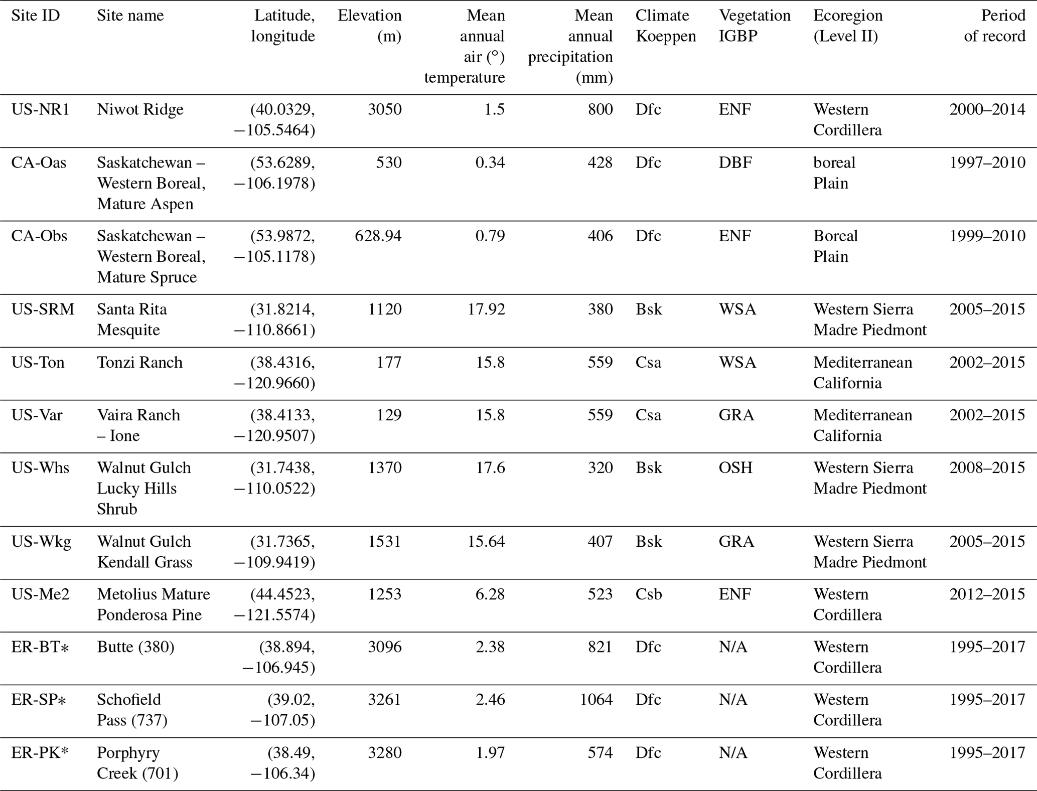
Figure 1 Location of sites considered in this study. Note that US-Ton and US-Var and US-Whs and US-Wkg are close to each other. East River Watershed is located next to ER-BT. The white lines delineate Western US states and Canadian provinces. Circles represent FLUXNET sites, diamonds represent SNOTEL sites, and the triangle represents the East River Watershed.

2.3 East River Watershed characteristics and previous analyses

Data from the East River Watershed were used to explore how ET and R_eco dynamics estimated from the developed HPM vary with different vegetation and meteorological forcings. The East River Watershed is located northeast of the town of Crested Butte, Colorado. This watershed has an average elevation of 3266 m, with significant gradients in topography, hydrology, geomorphology, vegetation, and weather. The mean annual air temperature in the East River is ∼2.4 ^∘C, with average daily air temperatures of −7.6 and 13.4 ^∘C in December and July respectively (Kakalia et al., 2020) and an average of 1200 mm yr⁻¹ total precipitation (Hubbard et al., 2018). Consisting of montane, subalpine, and alpine life zones, each with distinctive vegetation biodiversity, the East River Watershed is a test bed for the US Department of Energy Watershed Function Scientific Focus Area Project, led by the Lawrence Berkeley National Laboratory (Hubbard et al., 2018). The project has acquired a range of datasets, including hydrological, biogeochemical, remote-sensing, and geophysical datasets.

Recently completed studies at the East River Watershed were used in this study to inform HPM and to assess the results. For example, physically model-based estimations of ET at this site (Tran et al., 2019) were used herein for HPM development and validation. Falco et al. (2019) used machine-learning-based remote-sensing methods to characterize the spatial distribution of vegetation types, slopes, and aspects within a hillslope at the East River Watershed, which were used with obtained HPM estimates to explore how vegetation heterogeneity influences ET and R_ECO dynamics. To perform this assessment, we computed the spatial distribution of vegetation types at watershed scale based on Falco et al. (2019). We evaluated manually and selected 16 locations within the East River Watershed having different vegetation types and slope aspects. These 16 locations were chosen to be at the center of vegetation patched and covered by one vegetation type. A summary of the locations is presented in Table 2; the spatial distribution of the locations is shown in Fig. 2.

Table 2 Location and vegetation types of East River Watershed sampling points (Fig. 2).

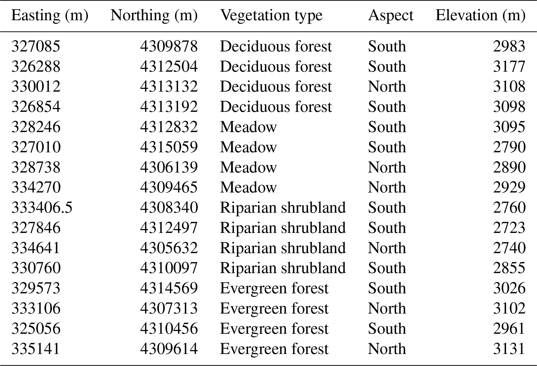
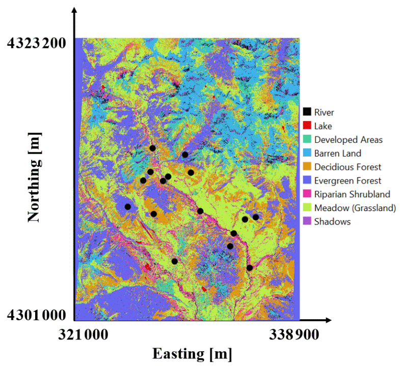
Figure 2 Vegetation classification of the East River Watershed, CO, from Falco et al. (2019). East River sites selected in this study are denoted by black circles.

2.4 Data collection and processing

To enhance transferability of the developed HPM strategy to less intensively characterized watersheds, we selected only “easy to measure” or “widely available” attributes, such as precipitation, air temperature, radiation, and NDVI, as inputs to the HTM model. Soil temperature was used when available. The data sources used for these inputs include FLUXNET data (https://fluxnet.fluxdata.org/, last access: 1 July 2020), SNOTEL data (https://www.wcc.nrcs.usda.gov/snow/, last access: 1 July 2020) and developed CLM model (Tran et al., 2019) at SNOTEL stations, DAYMET meteorological inputs (Thornton et al., 2017), and remote-sensing data from Landsat imageries (Irons et al., 2012). We identified some data gaps and erroneous data (especially during winter seasons) for the ET estimates at US-NR1, which were cleaned following the procedures presented in Rungee et al. (2019). At the three selected SNOTEL stations, air temperature data at these three SNOTEL stations were processed following Oyler et al. (2015) and radiation data were obtained from DAYMET. CLM models were generated following Tran et al. (2019) for the SNOTEL stations and US-NR1. At the East River Watershed sites, data were obtained from DAYMET. NDVI time series were calculated from the red band and near-infrared band from Landsat 5, 7, and 8 images at all sites. We used the cloud-scoring algorithm provided in the Google Earth Engine to mask clouds in all retrieved data, only selecting the ones that had a simple cloud score below 20 to ensure data quality. Given the different calibration sensors used in Landsat 5, 7, and 8, we also followed the processes described in Homer et al. (2015) and Vogelmann et al. (2001) to keep NDVI computations consistent over time. Landsat satellites have a return period of 16 d, and thus we performed a reconstruction of NDVI time series to obtain daily-scale time data (Sect. 3.2.2).

3 Hybrid predictive modeling framework

In this section, we illustrate the steps for building an HPM model for ET and R_eco estimation over time and space. Figure 3 presents the general framework of HPM, which includes modules for data preprocessing, model development, model validation, and predictive modeling.

3.1 Model framework

HPM establishes relationships among meteorological forcings' attributes, NDVI, ET, and R_eco (Fig. 3) using a deep-learning-based module (fully connected deep neural networks and long short-term memory recurrent neural networks). Long short-term memory (LSTM; Hochreiter and Schmidhuber, 1997) is a type of recurrent neural network (RNN) capable of learning temporal dependence without suffering from optimization difficulties (e.g., vanishing errors). An LSTM layer consists of memory blocks and unique cell states that are controlled by three multiplicative units, including the input, output, and forget gates. These gates regulate the flow of information and decide which data in a sequence are important to keep or throw away. Through the LSTM structure, even information from the earlier time steps can make its way to later time steps, reducing the effects of short-term memory and thus capturing long-term dependence. LSTM has been previously used to capture such dependencies between climate and environmental data. For example, Kratzert et al. (2018) successfully used LSTM to learn the long-term dependencies in hydrological data (e.g., storage effects within catchments, time lags between precipitation inputs and runoff generation) for rainfall-runoff modeling. LSTM has also been used for gap filling in hydrological monitoring networks in the spatiotemporal domain (Ren et al., 2019). More information about the LSTM-RNN method is provided by Olah (2015).

HPM modules include input attributes, model development, validation, and prediction. Based on data availability, input features are obtained from flux towers, CLM predictions, gridded meteorological data, and remote-sensing data; all data are preprocessed for gap filling, smoothing, and updating. In the HPM model development module, individual HPM models can be trained in two different ways based on data availability: with data obtained from flux towers (“data-driven HPM”) or with outputs from physically based models (“mechanistic HPM”). A proportion of 70 % of these data are used for training LSTM to learn the interactions among input features, ET, and R_eco, until a predefined “stopping criteria” (e.g., root mean squared error, RMSE) is met, indicating subsequent training would lead to minimal improvement. In most models, the configuration of the neural networks includes a first LSTM layer with 50 units, a second LSTM layer with 25 units, a dense layer with 8 units having L2 regularizers, and a final output dense layer. Dropout layers are also embedded in the model to prevent overfitting. There are 11600 and 7600 parameters for the first and second LSTM layers, 208 and 9 for the first and second dense layers, and no parameters for the dropout layers. Other configurations of networks may provide better estimation results; however, they are not assessed in this study as the proposed configuration already provide reasonable results.

In the validation module, we implemented a validation procedure that uses the remaining 30 % of the data to assess model performance. Estimation outputs from the trained HPM models are also compared with other ET and R_eco data obtained from other independent sites or mechanistic models within the same ecoregion. Statistical measures such as adjusted R² and mean absolute error (MAE) are computed to evaluate the performance of HPM models. In the predictive model module, meteorological forcings data and remote-sensing data are processed at target sites of interest, and the validated HPM model is used to estimate ET and R_eco at these sites. ET and R_eco outputs estimated from HPM at sparsely monitored watersheds then provide alternative datasets for process understanding within the target watersheds.

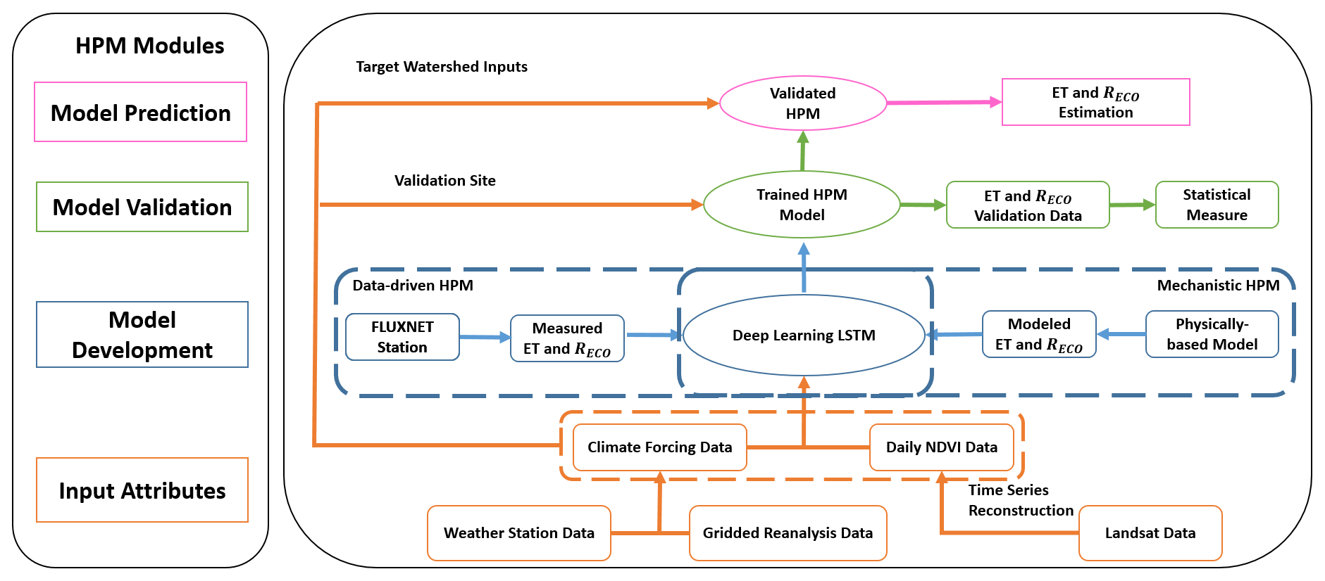
Figure 3 Hybrid predictive model (HPM) framework. The HPM model mainly consists of four modules: input attributes, model development, model validation, and model prediction, represented by rectangles with colors. Arrows represent the linkages among different modules. Choices of data-driven HPM or mechanistic HPM depend on the ecoregion of target watershed and data availability.

3.2 Feature selection

At sparsely monitored watersheds, only weather reanalysis data and remote-sensing data are commonly available. Thus, we mainly considered air temperature, radiation, precipitation, vegetation indices (e.g., NDVI), and variables inferred from these data as inputs for HPM. Soil temperature when available is used at FLUXNET sites. Other key attributes that depend on depth- and site-specific characteristics such as soil moisture and snow depth are not used in current HPM models due to data availability.

3.2.1 Snow information

In snow-influenced mountainous watersheds, we separated precipitation data into snow precipitation (when air temperature <0) and rainfall precipitation (when air temperature >0), which is in line with what has been used in hydrological models such as CLM (Oleson et al., 2013). Knowles et al. (2016) discovered a significant correlation between day of peak snow accumulation, snowmelt, and air temperature. To capture snow-related dynamics (e.g., snowmelt), we constructed a categorical variable (sn) based on air and soil temperature thresholds. Note that this may not be needed if snow data become available and at sites where snow is rarely present.

$$\begin{array}{}\text{(1)}& \mathrm{sn}=\left\{\begin{array}{l}\mathrm{0},\mathrm{during}\mathrm{snow}\mathrm{accumulation};\mathrm{air}\\ \mathrm{temperature}<\mathrm{0}\\ \mathrm{1},\mathrm{during}\mathrm{snow}\mathrm{melting};\mathrm{air}\mathrm{temperature}\\ >\mathrm{0}\mathrm{while}\mathrm{soil}\mathrm{temperature}\le \mathrm{0}\\ \mathrm{2},\mathrm{no}\mathrm{snow};\mathrm{air}\mathrm{temperature}\mathrm{and}\mathrm{soil}\\ \mathrm{temperature}>\mathrm{0}\end{array}\right.,\end{array}$$

3.2.2 Vegetation information

We reconstructed daily NDVI values based on meteorological forcing data (e.g., air temperature, precipitation, radiation) using LSTM to increase the temporal coverage of NDVI as the current HPM configuration requires daily inputs. Figure 4 represents Landsat-derived NDVI and reconstructed NDVI values for two sites at the East River Watershed, CO: Butte (ER-BT) and Schofield Pass (ER-SP). Though not ideal, as satellites continue to advance and more training data becomes available, the accuracy of NDVI temporal reconstruction is expected to increase.

Figure 4 Temporal reconstruction of NDVI at ER-BT (a) and ER-SP (b). Black lines represent reconstructed daily NDVI. Red points are used for training, and blue points are used for validation.

3.3 Use cases

We developed four different use cases to demonstrate the applicability of the HPM approach based on site-specific data and model availability. Use case 1 focuses on ET and R_eco in the time domain, where a HPM is trained on direct measurements from flux tower. A 70 %–20 %–10 % training–validation–prediction split of the data was used. The HPM approach is useful for time series gap filling and future prediction. Use case 2 and use case 3 have emphasis on providing ET and R_eco over space, where use case 2 uses data-driven HPM and use case 3 utilizes mechanistic HPM. Data-driven HPM is trained with data from the flux tower, and mechanistic HPM is trained upon outputs from a mechanistic model (e.g., CLM). The HPM approach is usually trained at well-monitored watersheds where either flux data are available or data support the development of a mechanistic model. After training, this HPM approach integrates meteorological and remote-sensing inputs to provide ET and R_eco at target sparsely monitored watersheds within the same ecoregion. For both use case 2 and 3, we validated the HPM estimations against data from other sites within the same ecoregion. Use case 4 focuses on the East River Watershed, where we demonstrate how HPM can increase our understanding of ecosystem fluxes and explore the limitations of HPM in mountainous watersheds. Use case 4 estimations were validated against data extracted from other studies.

4 Results

4.1 Use Case 1: ET and R_ECO time series estimation with an HPM approach developed at FLUXNET sites

A local HPM approach was developed to estimate ET and R_eco using flux tower data obtained from FLUXNET sites listed in Table 1. At all FLUXNET sites, air temperature, precipitation, net radiation, NDVI, and soil temperature were used. For US-NR1, CA-Oas, and CA-Obs, sn is also included. The results, which are shown in Figs. 5 and A1–A4 and Table 3, reveal that the HPM approach was effective in estimating ET and R_eco. The long-term trends in ET and R_eco are well captured by HPM. However, short-term fluctuations in ET and R_eco during the summer periods are also not well captured by HPM. For example, at US-Ton and US-Var, we observed an increasing discrepancy in summertime ET and R_eco. This is mainly caused by insufficient training for summer extremes. At US-Me2, we observed significant increasing errors in the validation set, especially for R_eco, that are caused by significant differences in raw data between 2002–2010 (data used for training) and post-2011 (data used for validation).

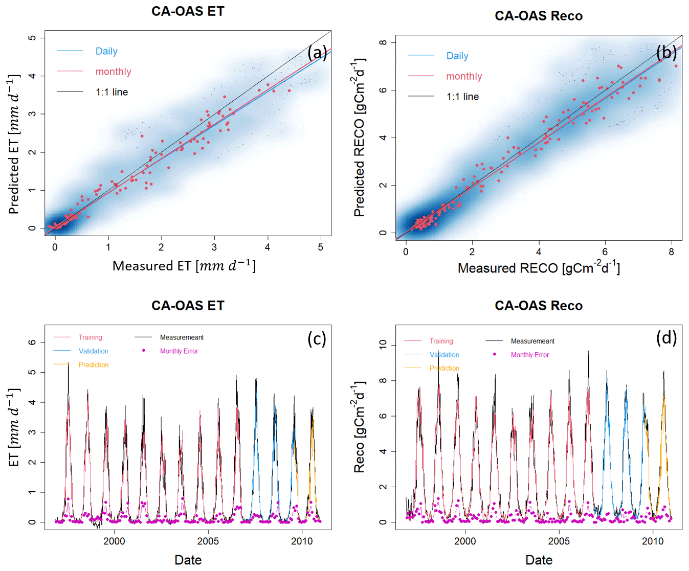
Figure 5 ET and R_eco estimation with data from FLUXNET sites at CA-OAS. Panels (a) and (b) show the scatter plots of daily (blue) and monthly (red) ET and R_eco between HPM estimation and FLUXNET data. Darker blue clouds represent greater density of data points. Panels (c) and (d) present the daily HPM estimation of ET and R_eco separated by training, validation and prediction sets. Pink points depict monthly error between HPM estimation and FLUXNET data. Results for other sites are included in the Appendices below (Figs. A1, A2, A3, and A4).

Table 3 Statistical measures of HPM estimation of ET and R_eco.

4.2 Use Case 2: ecoregion-based, data-driven HPM Model for ET and R_ECO estimation

In this section, we explored the use of a data-driven HPM trained with one FLUXNET station to estimate ET and R_eco at other locations within the same ecoregion. Specifically, we developed HPM models at US-Ton, CA-Oas, and US-Wkg and provided ET and R_eco estimations at US-Var, CA-Obs, and US-Whs at three ecoregions, respectively. Table 4 summarizes how we developed the data-driven HPM models for spatially distributed estimation of ET and R_eco as well as the corresponding statistical summaries. Figures 6 and A5 present the time series of HPM-estimated ET and R_ECO compared to measurements from flux towers. HPM estimation at US-Obs, US-Whs, and US-Var achieved an adjusted R² of 0.87, 0.88, and 0.91 for ET and 0.95, 0.70, and 0.78 for R_ECO, respectively. These results show that HPM captures the seasonal and long-term dynamics of ET and R_ECO However, at sites that experience seasonally dry periods (e.g., US-Whs), prediction accuracy decreases during the peak growing season. Although the prediction accuracy is not as high as Use Case 1 (Sect. 4.1), this use case demonstrates that HPM can learn the complicated relationships between responses and features successfully and that a local data-driven HPM can be used to fuse with data from other subsites for long-term estimation of ET and R_ECO within the same ecoregions.

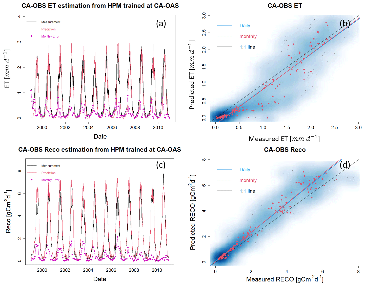
Figure 6 ET and R_eco estimation at CA-Obs using HPM trained at CA-Oas. Other sites are presented in Fig. A5.

4.3 Use Case 3: ecoregion-based, mechanistic HPM estimation of ET

Mechanistic HPM, which is trained upon physically based model simulations, provides an avenue for estimating fluxes in ecoregions where flux towers are not available. Consistent results between measured ET and CLM-estimated ET at US-NR1 (adjusted R²=0.88; k=0.95, Fig. S1) indicate independent CLM simulations can be effectively used to develop the mechanistic HPM. We applied mechanistic HPM trained with a 1-dimensional (vertical) CLM developed at ER-BT (Tran et al., 2019) to estimate ET at sites classified as part of the western Cordillera ecoregion (i.e., ER-SP, ER-PK, and US-NR1). We then compared ET estimation from HPM to independent CLM-based ET estimations at ER-SP and ER-PK. Figure 7 shows a high consistency between HPM estimation and the validation data. For all scenarios, an adjusted R² of 0.8 or greater is observed (Table 4), which strongly indicates that mechanistic HPM can provide accurate ET estimation at sites of similar ecoregions. These results suggest the broad applicability of mechanistic HPM to estimate ET based on ecoregion characteristics. This approach is expected to be particularly useful for regions where flux towers are difficult to install or where measured fluxes are not representative of the landscape, such as in mountainous watersheds.

Table 4 Statistical summary of HPM estimation over space with FLUXNET sites and SNOTEL stations with CLM.

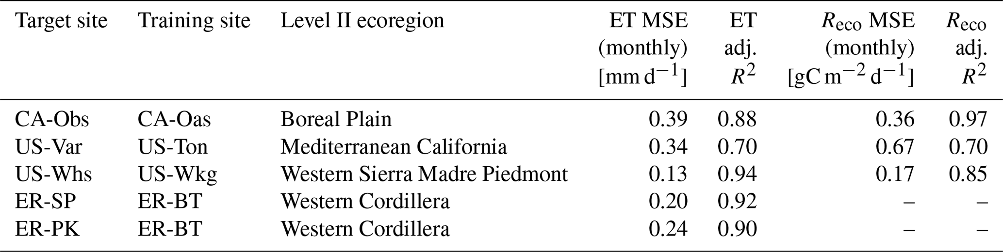
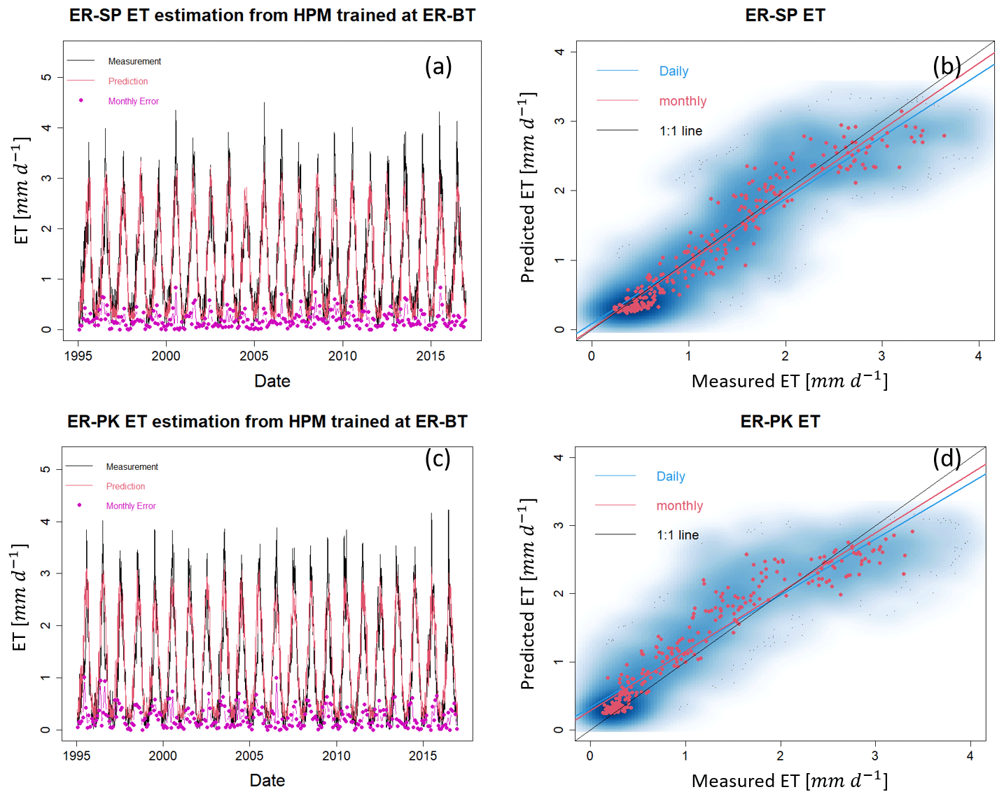
Figure 7 The HPM approach trained with CLM simulation at ER-BT is used to estimate ET at ER-SP and ER-PK. Panels (a) and (c) display the time series of HPM estimation of ET (red lines) and independent CLM estimation at ER-SP and ER-PK. Panels (b) and (d) show the scatter plots of daily (blue) and monthly (red) ET at these sites. Darker blue clouds represent greater density of data points.

4.4 Use Case 4: HPM approach improved our prediction capability and process understanding at the East River Watershed

With the proposed HPM approach (e.g., mechanistic HPM), we were able to estimate ET and R_eco at selected locations at the East River Watershed, CO, USA with only meteorological forcings and remote-sensing data. Our estimations are comparable to other independent studies, such as Mu et al. (2007) (Fig. S2) and Berryman et al. (2018). HPM estimations enhanced our understanding of watershed processes and enabled us to explore the limitations in the developed HPM approach especially at mountainous watersheds.

Physiology differences among vegetation types and dynamic changes in meteorological conditions were well captured by input features and HPM at the East River Watershed. Not surprisingly, the reconstructed NDVI indicated that deciduous forests have the highest peak NDVI, followed by grasslands, shrublands, and evergreen forests, whereas annual variation of NDVI in evergreen forests is smaller than the other vegetation types (Fig. 8). Year 2012 is regarded as a foresummer drought year with earlier than normal snowmelt, and year 2015 is regarded as a normal water year. The Palmer drought severity index (PDSI) is −5.2 and −1.5 for June and −4.6 and 1.1 for August in 2012 and 2015, respectively. Dynamic changes in meteorological conditions between 2012 and 2015 were also reflected in the reconstructed NDVI time series. We observed an earlier rise of NDVI in 2012: March, April, and May mean NDVI values for deciduous forest sites are 0.07, 0.2, and 0.37 compared to 0.06, 0.15, and 0.33 in 2015. Similar trends were observed for other vegetation types during spring months as well. NDVI values remain high during the peak growing season (deciduous forest > grassland > shrubland > evergreen forest) for both 2012 and 2015. However, we observed NDVI declines for grasslands and shrublands since August in 2012 but not until September in 2015. During autumn periods, NDVI declines significantly following the sharp decline in radiation.

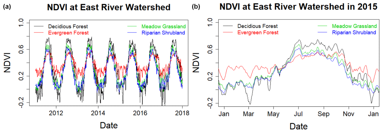
Figure 8 Reconstructed NDVI time series at selected locations in the East River Watershed for 2011 to 2018 (a) and for 2015 (b, normal water year). Black, red, green, and blue lines represent the time series of NDVI for deciduous forests, evergreen forests, meadow grasslands, and riparian shrubland, respectively.

HPM-estimated ET and R_eco also show different dynamics with different vegetation types and meteorological conditions. Figure 9a and b present the time series of estimated ET and R_eco associated with deciduous forests, respectively. Figure 9c and d present the ET and R_eco differences between deciduous forests sites and evergreen forests, shrublands, and grasslands. Before peak growing season, evergreen forests have the greatest ET and R_eco compared to the other vegetation types. ET of evergreen forests is about 10 % greater than deciduous forests, whereas ET of deciduous forests during peak growing season is greater than evergreen forests, shrublands and meadows. After growing season, the NDVI of deciduous forests is less than 0.2 (loss of leaves) compared to the NDVI of evergreen forests. Before peak growing season, R_eco of evergreen forests is slightly greater than deciduous forests, meadow grasslands, and shrublands. During peak growing season, we observed the largest R_eco for deciduous forests sites (∼6 gC m⁻² d⁻¹), followed by meadows, shrublands, and evergreen forests. R_eco of deciduous forests is around 17 % greater than R_eco of evergreen forests. However, we did not observe significant differences in annual ET among these four vegetation types (e.g., DF: 535 to 573 mm, MS: 534 to 570 mm, RS: 532 to 567 mm, and EF: 532 to 569 mm across 7 years in this study). Total annual R_eco of deciduous forests is greater than the other vegetation types (DF1: 642 to 698 gC m⁻², MS1: 588 to 636 gC m⁻², RS1: 589 to 636 gC m⁻², and EF1: 592 to 639 gC m⁻²). These results indicate HPM R_eco models are sensitive to vegetation types, and HPM ET models are mostly constrained by meteorological conditions.

Considering the inter-annual variability in meteorological forcings, we further selected year 2014 (large snow precipitation ∼587 mm but small rain precipitation ∼275 mm) in addition to 2012 (drought year) and 2015 (small snow precipitation ∼383 mm and large rain precipitation ∼477 mm) to test HPM performance. As HPM does not have the capability to identify the snow and monsoon precipitation contribution to fluxes, we separated annual ET and R_eco into pre-June (January–June) and post-July (July–December) to quantify the contribution from snow and monsoon. Earlier snowmelt that occurred in 2012 boosted spring ET and R_eco, and we observed larger March-mean ET and R_eco compared to 2014 and 2015, that are characterized by later snowmelt. Occurrences of foresummer drought in 2012 led to moisture-limiting conditions, resulting in large fluctuations of ET and R_eco during May and June. ET fluctuated from 2.9 to 1.9 mm d⁻¹ during late May and 3.53 to 2.6 mm d⁻¹ during early June. However, early occurrence of monsoon in 2012 led to a peak ET in early July. Due to late snowmelt, ET did not significantly fluctuate in 2014 and 2015. However, peak ET shifted towards late July in 2014. Regarding R_eco dynamics, foresummer drought conditions led to variations in R_eco from ∼4 to 6 gC m⁻² d⁻¹ in 2012. In 2014, we observed more steady increase of R_eco during the early and peak growing seasons. For late-summer and autumn months (August–October), ET decreased steadily in all 3 years regardless of monsoon precipitation inputs, following the significant decline in radiation. Pre-June ET and R_eco (255 mm and 217 gC m⁻² d⁻¹) were both greater in 2012 compared to 2014 (223 mm and 178 gC m⁻² d⁻¹) and 2015 (230 mm and 197 gC m⁻² d⁻¹) in deciduous forests. While there were no significant differences in post-July ET among the 3 years (318, 316, and 306 mm), 2012 was the highest. Within deciduous forests and annually over 2012, 2014, and 2015, ET was 573, 539, and 536 mm, and R_eco was 698, 642, and 652 gC m⁻², respectively. Similar trends were observed for other vegetation types.

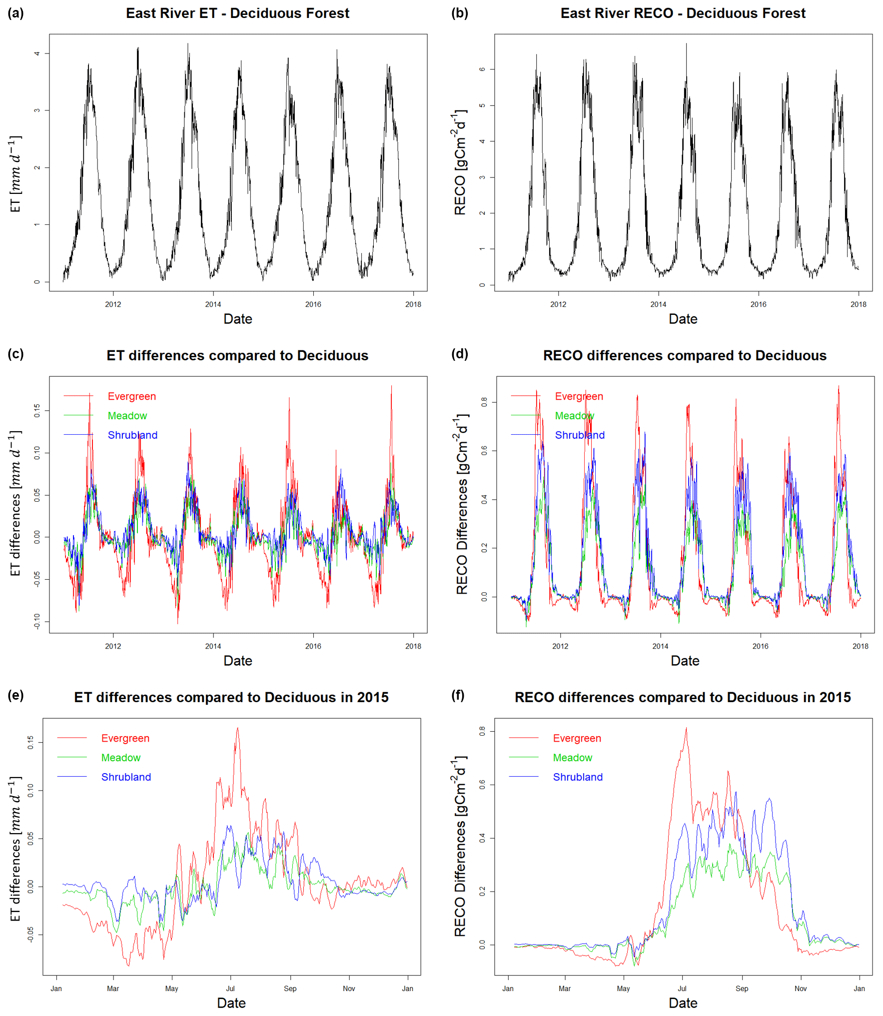
Figure 9 ET (a) and R_eco (b) estimation for the deciduous forest site DF1 at the East River Watershed. Panels (c) and (d) show the differences in ET and R_eco among various vegetation types and deciduous forest. Red, green, and blue lines represent the differences in evergreen forest, meadow, and riparian shrubland compared to deciduous forest. Panels (e) and (f) zoom into 2015 to better display seasonal variations.

Though HPM estimations allowed us to explore differences in ET and R_eco across vegetation and meteorological forcings heterogeneity, it is necessary to investigate the limitations of the HPM approach. Figure 10 shows the absolute value of monthly mean difference in ET (Fig. 10a and b) and R_eco (Fig. 10c and d) across SNOTEL stations (ER-BT, ER-SP and ER-PK) and within selected East River locations. We observed greater differences in air temperature and radiation at the SNOTEL sites but very small differences at the East River sites (Fig. S4). Differences in June air temperature among SNOTEL sites were occasionally over 3 ^∘C, while DAYMET data from the East River indicated 0.2 ^∘C differences. In addition, a radiation difference of ∼80 W m⁻² was observed with SNOTEL data compared to 30 W m⁻² for East River sites. As a result, ET differences across SNOTEL stations are 2.5 times greater than differences observed at the East River locations. A similar level of differences (around 0.8 gC m⁻²) was observed in R_eco within the East River Watershed and across SNOTEL stations. These results suggest the insufficient resolution of input meteorological forcing data at the East River sites have large uncertainties, which have a significant influence over HPM ET and HPM R_eco estimations. If high-resolution meteorological data become available for the East River watershed, we believe the HPM approach can better capture heterogeneities in ET and R_eco at the East River watershed and better distinguish the roles of meteorological forcing and vegetation heterogeneity in ET and R_eco distribution.

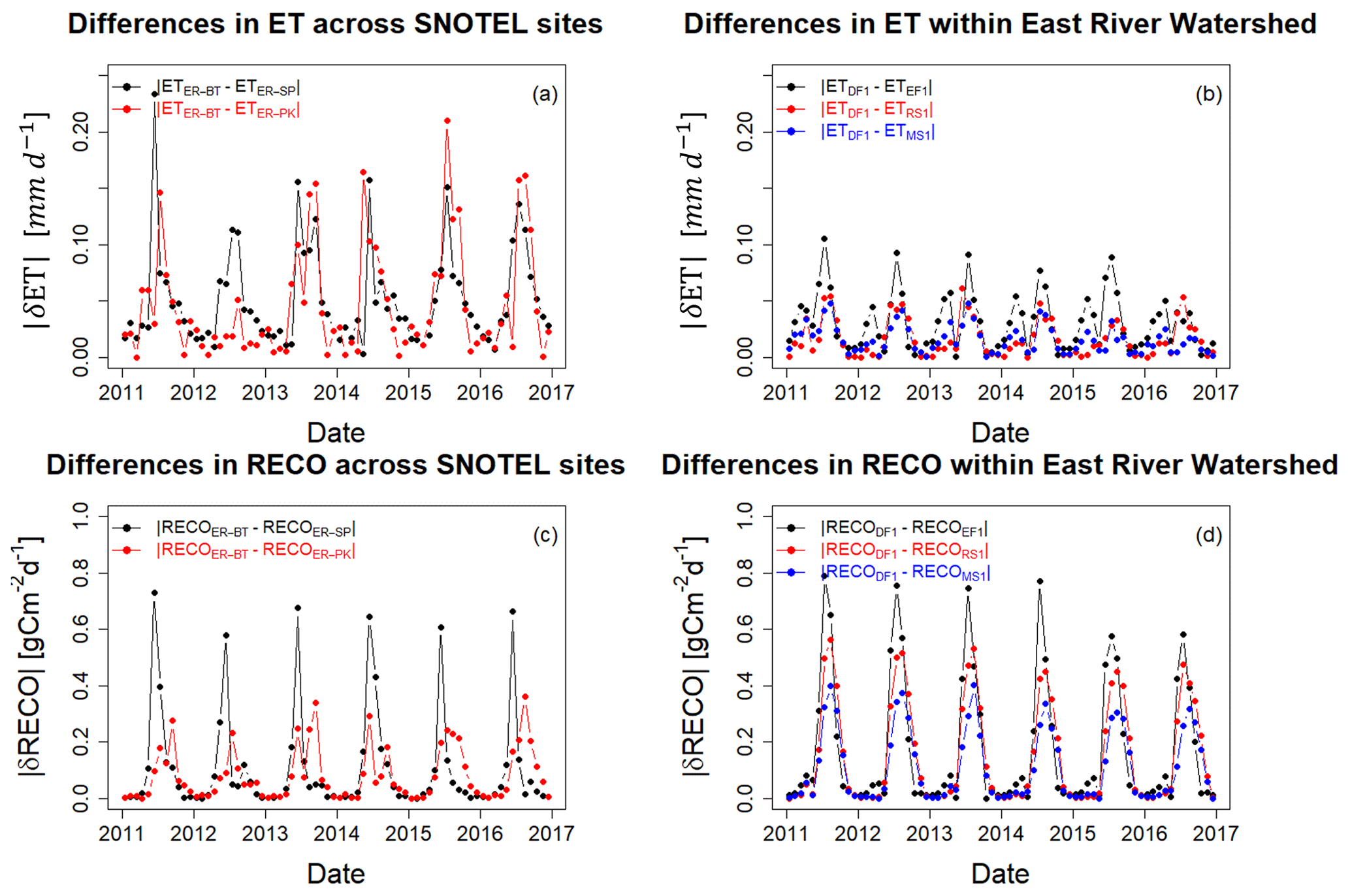
Figure 10 Absolute differences in monthly mean ET and R_eco across SNOTEL stations and within East River Watershed. Panels (a) and (c) describe the absolute differences in monthly mean ET and R_eco between ER-BT, ER-SP, and ER-PK. Panels (b) and (d) describe the absolute differences in monthly mean ET and R_eco within East River Watershed between deciduous forests, evergreen forests, meadow grasslands, and riparian shrublands.

5 Discussion

Our study demonstrates that HPM provides reliable estimations of ET and R_eco under various climate and vegetation conditions. The unique gated structures and cell states of LSTM allow HPM to track information from earlier times and decide which information to pass along and which information to forget. This effective configuration allows LSTM to effectively capture the long-term dependencies and ecological memory effects among meteorological forcings, NDVI, ET, and R_eco. With 70 % of the data used for training (model development), ET and R_eco estimation from HPM achieves an average adjusted R² of 0.9 compared to flux tower measurements. To demonstrate HPM's applicability for providing ET and R_eco estimation at sparsely monitored watersheds, we presented four use cases, including prediction ET and R_eco in the time domain, a data-driven HPM approach, and a mechanistic HPM approach. Results from the four use cases suggest HPM is a powerful approach to estimate ET and R_eco at target watersheds, requiring only five commonly available input data, and can advance our understanding of watershed processes.

HPM was capable of incorporating information from NDVI time series to delineate the physiological differences among deciduous forests, evergreen forests, shrublands, and grasslands. In our study, NDVI data indicated evergreen forests have a longer growing season compared to other vegetation types, and deciduous forests have higher peak NDVI values. Correspondingly, we also observed an earlier increase in ET and R_eco for evergreen forests (before May) but larger ET and R_eco for deciduous forests during peak growing season (around June and July). Baldocchi et al. (2010) found that deciduous forests had a shorter growing season but showed a greater capacity for assimilating carbon during the growing season. Evergreen forests, on the other hand, had an extended growing season but with a smaller capacity for gaining carbon. They found older leaves tend to have smaller leaf nitrogen and stomata conductance that lead to smaller ET and R_eco during peak growing seasons. Hu et al. (2010) found that extended growing season length resulted in less annual CO₂ uptake at Niwot Ridge, USA. They found increasing growing season length is usually correlated with decreasing snow water storage and decreasing forest carbon uptake. Xu et al. (2020) suggested canopy photosynthetic capacity is the driving force that leads to different resource use efficiencies (RUEs) between deciduous forests and evergreen forests. Novick et al. (2015) focused on the net ecosystem exchange of CO₂ and also suggested seasonality is less important for evergreen forests, where significant amounts of carbon were assimilated outside of the active season. These findings are consistent with what we found in HPM estimations, where we observed a greater ET and R_eco contribution during early and later seasons for evergreen forests compared to deciduous forests that have significantly greater peak ET and R_eco during peak growing season. As HPM only requires five input features, and NDVI is the only variable related with vegetation types, we were not able to perform detailed analysis delineating the physiological control on ET and R_eco dynamics. But we believe HPM models are still useful as they can provide initial ET and R_eco estimation that helps with site selection and field campaign designs.

Temporal variability in meteorological conditions also leads to unique ET and R_eco responses at the East River Watershed, as shown by HPM estimations. A total of 3 years with a diverse combination of snow and rain precipitation were analyzed. In 2012, a year that experienced earlier snowmelt, both ET and R_eco increased early in the season. However, earlier growth in vegetation and increasing demand for water resulted in foresummer drought conditions that led to decreases in ET and R_eco in late May and June. In 2014, HPM estimated a steady increase in ET and R_eco during spring months following radiation and air temperature trends, with no subsequent significant decline in ET and R_eco. This indicates that energy was still the key limiting factor for spring dynamics in 2014, leading to a smaller pre-June ET and R_eco compared to 2012. Following an earlier arrival of monsoon in 2012 compared to 2014 and 2015, we observed higher mean ET and R_eco in July than in June, which indicates the earlier arrival of monsoon precipitation greatly reduced the moisture limiting condition caused by foresummer drought and led to subsequent increase in ET and R_eco. During late-summer and autumn months, radiation declined significantly, with a ∼30 % decrease in August and ∼40 % decrease in September. Though 2012, 2014, and 2015 had diverse monsoon precipitation during these periods, HPM did not estimate significant differences in post-July ET. This result indicates the East River watershed is mainly under energy-limiting rather than moisture-limiting conditions during late-summer and autumn; and timing of monsoon arrival is more important than the absolute amount of monsoon precipitation for ET dynamics. This result is consistent with findings in Carroll et al. (2020). Their study also indicated an earlier arrival of summer monsoon was effectively supporting ET and that the monsoon precipitation was quickly consumed by vegetation, whereas a later arrival of summer monsoon water mainly contributed to streamflow under energy-limiting conditions.

Uncertainties of HPM models arise from several aspects. First, the current choice of only five input features based on data availability may decrease estimation accuracy in certain environments, such as sites with seasonally dry periods. Though the LSTM component within the HPM approach can capture the memory effects and long-term dependencies of watershed dynamics, rare extreme values are difficult to be captured by LSTM due to insufficient training data for such cases. For example, we observed a decreasing prediction accuracy for ET and R_eco estimation at sites that experience drought conditions. Current use of meteorological forcings data and NDVI may not provide sufficient data for LSTM to identify droughts implicitly. Other key variables (e.g., soil moisture) when available can potentially be useful to help LSTM better quantify these rare events and increase model performance. Secondly, parameterization and insufficient spatiotemporal resolution of meteorological data still remain a challenge. Field observations along the Rocky Mountain ranges have shown that south-facing hillslopes have significantly earlier snowmelt compared to north-facing hillslopes (Kampf et al., 2015; Webb et al., 2018). However, we did not observe the same level of heterogeneities in radiation and air temperature in reanalysis data compared to weather station data (Figs. S4 and S5). Mu et al. (2007) and Zhang et al. (2019) suggested uncertainties in meteorological inputs can result in large errors (i.e., >20 % MAE) and reduce accuracy by 10 %–30 %. Additionally, HPM is also influenced by remote-sensing inputs' accuracy, including but not limited to insufficient resolution, cloud conditions, spatial averaging, temporal reconstruction, and any other algorithms involved. But with recent advances in remote-sensing and satellite technologies (McCabe et al., 2017) and harmonized Landsat–Sentinel datasets (Claverie et al., 2018), the spatial and temporal resolution should greatly increase in the future (i.e., 3 m resolution and daily). Finally, errors can stem from the HPM hybrid approaches and conceptual model uncertainties. Any original errors in mechanistic models will be passed onto HPM estimations of ET and R_eco. We recommend training a data-driven HPM approach and a mechanistic HPM approach using long time series (e.g., >5 years) with high-quality data or simulations, which enables the HPM approach to better memorize long-term dependencies of ecosystem dynamics. Though some of the uncertainties still remain a challenge, efforts have been made to minimize them through the technical advances described herein. Future HPM models can potentially be jointly trained on FLUXNET and process-based simulations to bypass certain limitations and provide more accurate ET and R_eco at sparsely monitored watersheds.

6 Conclusions

In this study, we developed and tested a hybrid predictive modeling approach for ET and R_eco estimation, with an enhanced focus on a watershed in the Rocky Mountains. We developed individual HPM models at various FLUXNET sites and at sites where data could support the proper development of a mechanistic model (e.g., CLM). These models were trained and validated against eddy covariance measurements and CLM outputs. We further used these models for ET and R_eco estimation at watersheds within the same ecoregion to test HPM's capability of providing estimation over space, where only meteorological forcings data and remote-sensing data were available. Lastly, we applied the HPM to provide long-term estimation of ET and R_eco and test the sensitivity of HPM to various vegetation and meteorological conditions within the East River Watershed of CO, USA.

Given the promising results of HPM, the approach offers an avenue for estimating ET and R_eco using easy-to-acquire or commonly available datasets. This study also suggests that the spatial heterogeneity of meteorological forcings and vegetation dynamics has significant impacts on ET and R_eco dynamics, which may be currently underestimated due to the typically coarse spatial resolution of data inputs. Parameters related to energy and soil moisture conditions can be implemented into HPM to increase HPM's accuracy, especially for sites in ecoregions limited by soil moisture conditions. Lastly, it should be pointed out that HPM is not restricted to estimation of ET and R_eco only. HPM also has great potential for estimating other parameters important for water and carbon cycles given the right choice of input variables, such as net ecosystem exchange (Fig. B1). Thus, we believe the proposed HPM model can improve our prediction capabilities of ET and R_eco at sparsely monitored watersheds and advance our understanding of watershed dynamics.

Appendix A: ET and R_ECO estimation over time at other FLUXNET sites

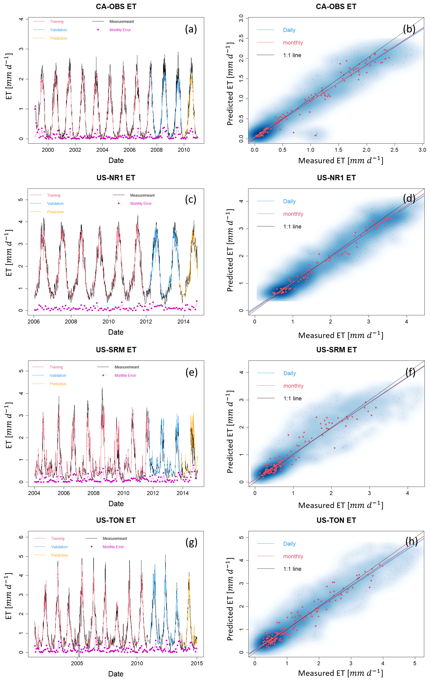
Figure A1 ET estimation with data from selected FLUXNET sites at CA-OBS, US-NR1, US-SRM, and US-Ton. Panels (a), (c), (e), and (g) present daily estimations of ET separated for training, validation, and prediction. Pink points depict monthly error between HPM estimation and FLUXNET data. Panels (b), (d), (f), and (h) show the scatter plots of daily (blue) and monthly (red) ET. Darker blue clouds represent a greater density of data points.

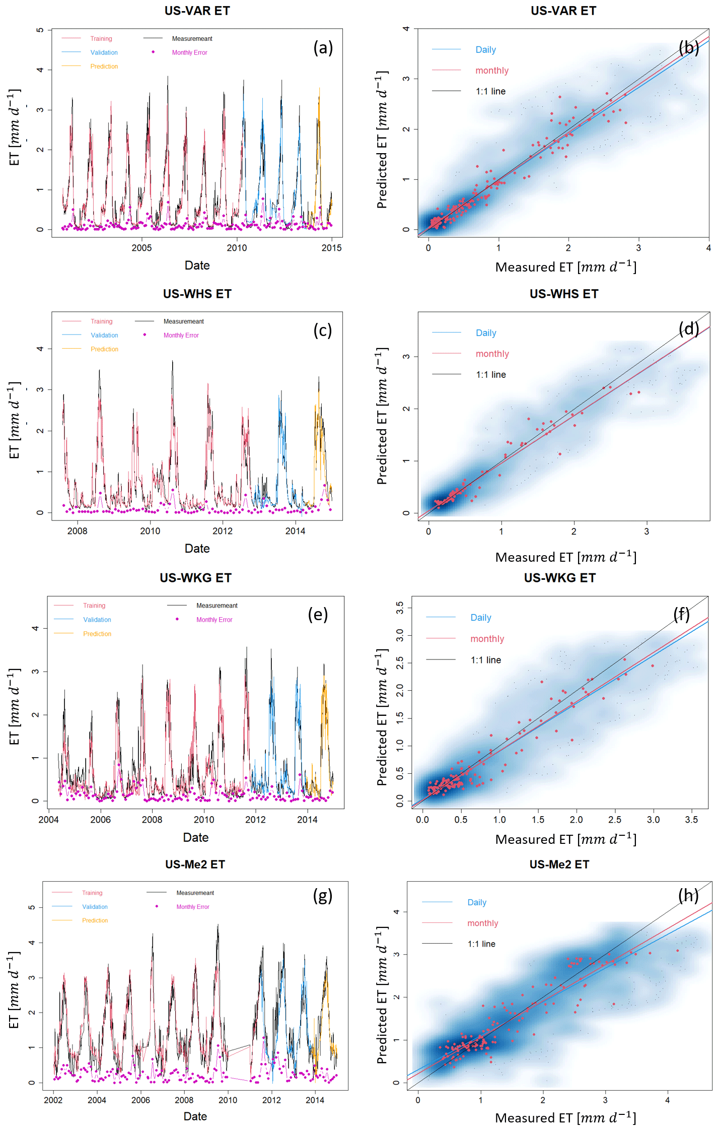
Figure A2 ET estimation with data from selected FLUXNET sites at US-Var, US-Whs, US-Wkg, and US-Me2. Panels (a), (c), (e), and (g) present daily estimations of ET separated for training, validation, and prediction. Pink points depict monthly error between HPM estimation and FLUXNET data. Panels (b), (d), (f), and (h) show the scatter plots of daily (blue) and monthly (red) ET. Darker blue clouds represent a greater density of data points.

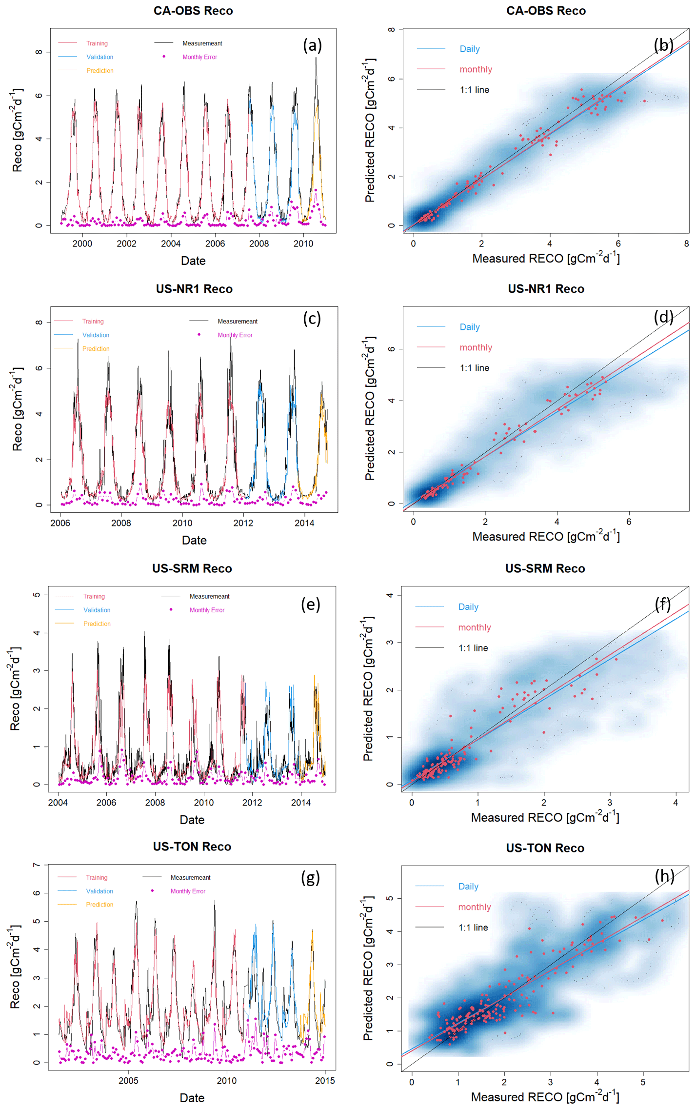
Figure A3 R_eco estimation with data from selected FLUXNET sites at CA-OBS, US-NR1, US-SRM, and US-Ton. Panels (a), (c), (e), and (g) present daily estimations of R_eco separated for training, validation, and prediction. Pink points depict monthly error between HPM estimation and FLUXNET data. Panels (b), (d), (f), and (h) show the scatter plots of daily (blue) and monthly (red) R_eco. Darker blue clouds represent a greater density of data points.

Figure A4 R_eco estimation with data from selected FLUXNET sites at US-Var, US-Whs, US-Wkg, and US-Me2. Panels (a), (c), (e), and (g) present daily estimations of R_eco separated for training, validation, and prediction. Pink points depict monthly error between HPM estimation and FLUXNET data. Panels (b), (d), (f), and (h) show the scatter plots of daily (blue) and monthly (red) R_eco. Darker blue clouds represent a greater density of data points.

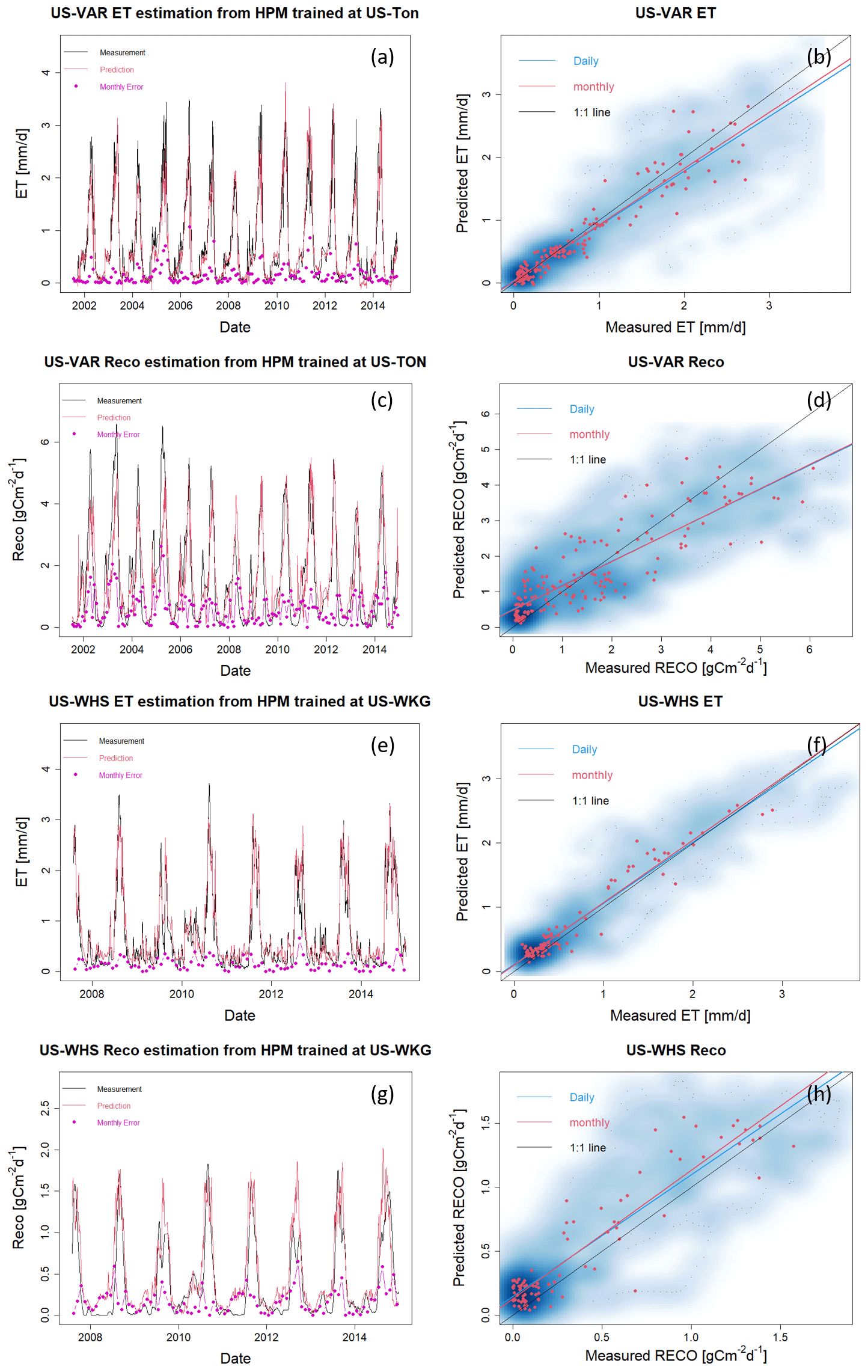
Figure A5 Use case 2. ET and R_eco estimation at US-Var and US-Whs from HPM trained at US-Ton and US-Wkg, respectively.

Appendix B: Tested NEE estimation over time at CA-OAS and US-NR1

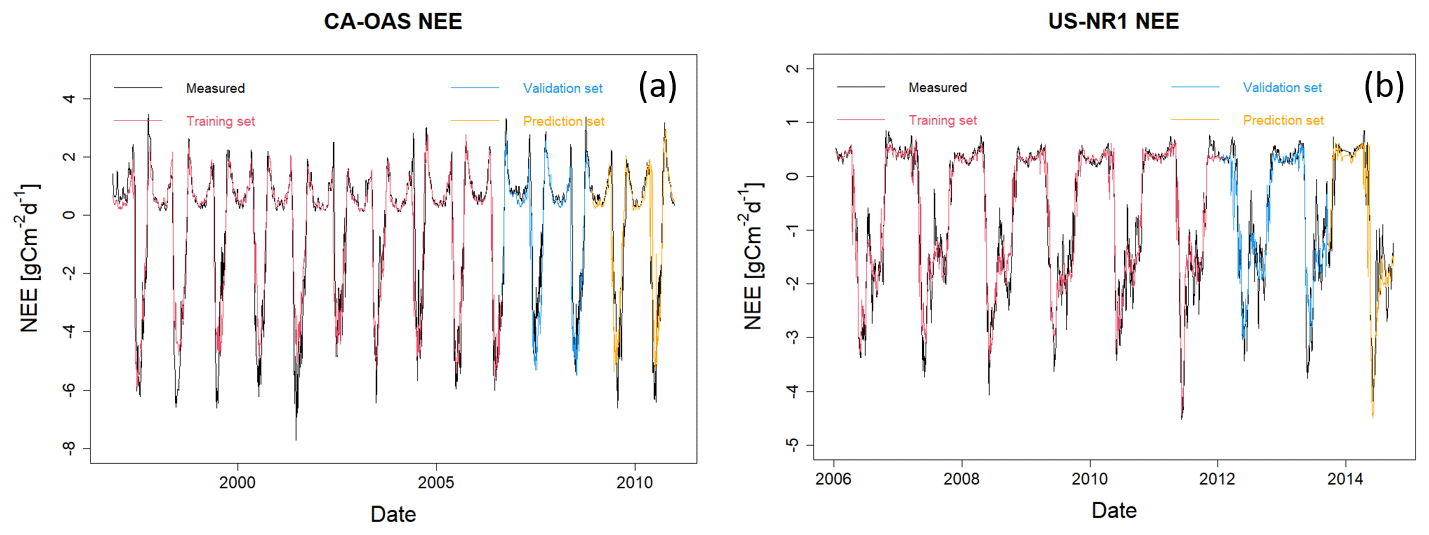
Figure B1 HPM estimate of NEE at CA-OAS and US-NR1. R² values between estimation and measurements are 0.87, 0.83, and 0.81 at CA-OAS and 0.94, 0.88, and 0.90 at US-NR1 for the training set, validation set, and prediction set, respectively. Model inputs include air temperature, soil temperature, sn, precipitation, and radiation.