the Creative Commons Attribution 4.0 License.
the Creative Commons Attribution 4.0 License.
 | 10 Feb 2021
Comparative analysis of kernel-based versus ANN and deep learning methods in monthly reference evapotranspiration estimation
Mohammad Taghi Sattari
Halit Apaydin
Shahab S. Band
Amir Mosavi
Ramendra Prasad
Timely and accurate estimation of reference evapotranspiration (ET0) is indispensable for agricultural water management for efficient water use. This study aims to estimate the amount of ET0 with machine learning approaches by using minimum meteorological parameters in the Corum region, which has an arid and semi-arid climate and is regarded as an important agricultural centre of Turkey. In this context, monthly averages of meteorological variables, i.e. maximum and minimum temperature; sunshine duration; wind speed; and average, maximum, and minimum relative humidity, are used as inputs. Two different kernel-based methods, i.e. Gaussian process regression (GPR) and support vector regression (SVR), together with a Broyden–Fletcher–Goldfarb–Shanno artificial neural network (BFGS-ANN) and long short-term memory (LSTM) models were used to estimate ET0 amounts in 10 different combinations. The results showed that all four methods predicted ET0 amounts with acceptable accuracy and error levels. The BFGS-ANN model showed higher success (R2=0.9781) than the others. In kernel-based GPR and SVR methods, the Pearson VII function-based universal kernel was the most successful (R2=0.9771). Scenario 5, with temperatures including average temperature, maximum and minimum temperature, and sunshine duration as inputs, gave the best results. The second best scenario had only the sunshine duration as the input to the BFGS-ANN, which estimated ET0 having a correlation coefficient of 0.971 (Scenario 8). Conclusively, this study shows the better efficacy of the BFGS in ANNs for enhanced performance of the ANN model in ET0 estimation for drought-prone arid and semi-arid regions.
- Article
(563 KB) - Full-text XML
- BibTeX
- EndNote


Accurate estimation of reference crop evapotranspiration (ET0) and crop water consumption (ET) is essential in managing water in the agricultural sector particularly for arid and semi-arid climatic conditions where water is scarce and valuable. Although ET0 is a complex element of the hydrological cycle, it is also an important component of hydro-ecological applications and water management in the agricultural sector. The estimation of ET0 is critical in the forcible management of irrigation and hydro-meteorological studies on respective basins and on national scales (Pereira et al., 1999; Xu and Singh, 2001; Anli, 2014) since knowledge of ET0 would allow for reduced water wastage, increased irrigation efficiency, proper irrigation planning, and reuse of water.
In general, the equations that calculate ET0 values are very complex, nonlinear, contain randomness, and all in all have several underlying assumptions. The results obtained from these equations differ greatly from the measured values. ET0 is considered a complex and nonlinear phenomenon that interacts with water, agriculture, and climate. It is difficult to emulate such a phenomenon by experimental and classical mathematical methods. About 20 well-known methods for estimating ET0 based on different meteorological variables and assumptions are available in the literature. The Penman–Monteith (FAO56PM) method proposed by FAO is recommended to estimate ET0, as it usually gives usable results in different climatic conditions (Hargreaves and Samani, 1985; Rana and Katerji, 2000; Feng et al., 2016; Nema et al., 2017). Cobaner et al. (2017) modified the Hargreaves–Samani (HS) equation used in the determination of ET0. Solving the equations and finding the correct parameter values requires sophisticated programs for the employment of differential equations, which require rigorous optimization methods together with a broad range of high-quality and accurate spatio-temporal input data with the knowledge of initial conditions (Prasad et al., 2017).
On the other hand, the developments in artificial intelligence (AI) methods and the increase in the accuracy of the estimation results have increased the desire for these AI methods. The AI models offer a number of advantages including their ease of development compared to physically-based models, not requiring underlying boundary conditions or other assumptions or initial forcings, and the ability to operate at localized positions (Prasad et al., 2020). Consequently, many studies have been reported to have applied AI approaches for ET0 estimations. Artificial intelligence techniques based on machine learning (ML) has been successfully utilized in predicting complex and nonlinear processes in natural sciences, especially hydrology (Koch et al., 2019; Prasad et al., 2017; Solomatine, 2002; Solomatine and Dulal, 2003; Yaseen et al., 2016; Young et al., 2017). Thus, methods such as ML and deep learning have gained popularity in estimating and predicting ET0.
The artificial neural network (ANN) has been the most widely used ML model to date. Sattari et al. (2013) used the backpropagation algorithm of the ANN and tree-based M5 model to estimate the monthly ET0 amount by employing a climate dataset (air temperature, total sunshine duration, relative humidity, precipitation, and wind speed) in the Ankara region and compared the estimated ET0 with FAO56PM computations. The results revealed that the ANN approach gives better results. In another study, Pandey et al. (2017) employed ML techniques for ET0 estimation using limited meteorological data and evaluated evolutionary regression (ER), ANN, multiple nonlinear regression (MLNR), and SVM. They found that the ANN FAO56PM model performed better. In their study, Nema et al. (2017) studied the possibilities of using an ANN to increase monthly evapotranspiration prediction performance in the humid area of Dehradun. They developed different ANN models, including combinations of various training functions and neuron numbers, and compared them with ET0 calculated with FAO56PM. They found that the ANN trained by the Levenberg–Marquardt algorithm with 9 neurons in a single hidden layer made the best estimation performance in their case. The ANNs with multiple linear regression (MLR), ELM, and HS models were tested by Reis et al. (2019) to predict ET0 using temperature data in the Verde Grande River basin, Brazil. The study revealed that AI methods have superior performance over other models. Abrishami et al. (2019) estimated the amount of daily ET0 for wheat and corn using ANNs and found the proper and acceptable performance of ANNs with two hidden layers. However, some studies showed a slightly better performance of other models. Citakoglu et al. (2014) predicted monthly average ET0 using the ANN and adaptive network-based fuzzy inference system (ANFIS) techniques using combinations of long-term average monthly climate data such as wind speed, air temperature, relative humidity, and solar radiation as inputs and found ANFIS to be slightly better than ANN. Yet they found both methods to be successful in estimating the monthly mean ET0. Likewise, ANN and ANFIS models employing the cuckoo search algorithm (CSA) were applied by Shamshirband et al. (2016) using data from 12 meteorological stations in Serbia. The results showed that the hybrid ANFIS-CSA could be employed for high-reliability ET0 estimation.
Despite ANNs being universal approximators with the ability to approximate any linear or nonlinear system without being constrained to a specific form, there are some inherent disadvantages. Slow learning speed, over-fitting, and constraints in local minima make it relatively tedious to determine key parameters, such as training algorithms, activation functions, and hidden neurons. These inherent structural problems sometimes make ANNs difficult to adapt for different applications. However, despite all the disadvantages, it is still a preferred method in all branches of science and especially in hydrology. Having said that, in this study, the ANN is benchmarked with other comparative models. One such model is support vector machine (SVM) developed by Vapnik (2013). SVMs have good generalization ability since they utilize the concept of the structural risk minimization hypothesis in minimizing both empirical risk and the confidence interval of the learning algorithm. Due to the underlying solid mathematical foundation of statistical learning theory giving it an advantage, the SVMs have been preferred in a number of studies and produced highly competitive performances in real-world applications (Quej et al., 2017). Subsequently, Wen et al. (2015) predicted daily ET0 via SVM, using a limited climate dataset in the Ejina Basin, China, using the highest and lowest air temperatures, daily solar radiation, and wind speed values as model inputs and FAO56PM results as model output. The SVM method's performance was compared to ANN and empirical techniques, including Hargreaves, Priestley–Taylor, and Ritchie, which revealed that the SVM recorded better performance. Zhang et al. (2019) examined SVM's success in ET0 estimation and compared the outcomes with Hargreaves, FAO-24, Priestley–Taylor, McCloud, and Makkink. SVM was determined to be the most successful model. However, SVM also has several drawbacks, such as having a high computational memory requirement as well as being computational exhaustive, as a large amount of computing time is necessary during the learning process.
In order to overcome the disadvantages of these two widely accepted approaches (ANN and SVM), many new modelling techniques have been proposed in recent years. For instance, the two state-of-the-art machine learning techniques, namely Gaussian process regression (GPR) and long short-term memory (LSTM), have also been recently trialled in hydrologic time series modelling and forecasting applications. Following the newer developments, Shabani et al. (2020) used ML methods, including GPR, random forest (RF), and SVR, with meteorological inputs to estimate evaporation in Iran and found that ML methods have high performances even with a small number of meteorological parameters. In a recent study, deep learning and ML techniques to determine daily ET0 have been explored in Punjab's Hoshiarpur and Patiala regions, India (Saggi et al., 2019). They found that supervised learning algorithms such as the deep learning (DL) multilayer sensor model offers high performance for daily ET0 modelling. However, to the best of the authors' knowledge, there have been very few attempts to test the practicability and ability of these two advanced approaches (LSTM and GPR) for ET0 modelling and prediction. In addition, many studies included solar radiation in the modelling process yet did not include sunshine hours in the modelling, which will be dealt with in this study.
With recent developments in ML methods with the use of deep learning techniques such as LSTM in water engineering together with technical developments in computers and the emergence of relatively comfortable coding languages, this study explores the application of different deep learning (LSTM) and other machine learning methods (ANN, SVM, and GPR) in the estimation of ET0 to shed light on future research and to determine effective modelling approaches relevant to this field. ET0 is one of the essential elements in water, agriculture, hydrology, and meteorology studies, and its accurate estimation has been an open area of research due to ET0 being a complex and nonlinear phenomenon. Hence, robust deep learning and ML approaches including LSTM, ANN, SVM, and GPR methods need to be aptly tested. As a result, this study has three important goals: (i) to estimate the amount of ET0 using deep learning and machine learning methods, i.e. GPR, SVR, and Broyden–Fletcher–Goldfarb–Shanno ANN (BFGS-ANN) learning algorithms, as well as LSTM in Corum, Turkey, an arid and semi-arid climatic region with a total annual rainfall of 427 mm; (ii) to investigate the effect of different kernel functions of the SVR and GPR models on the performance of ET0 estimation; and (iii) to determine the model that provides the highest performance with the fewest meteorological variable requirements for the study. A proper prediction of reference evapotranspiration would be vital in managing limited water resources for optimum agricultural production.
Corum encompasses an area of 1 278 381 ha, of which 553 011 ha, or 43 %, is agricultural land (Fig. 1). Its population is 525 180, and 27 % of it lives in rural areas. The city's water resource potential is 4916 hm3 yr−1, and 84 988 ha of agricultural land is being irrigated. The main agricultural products are wheat, paddy, chickpeas, onions, walnuts, and green lentils. This study was conducted using monthly meteorological data including highest and lowest temperature; sunshine duration; wind speed; and average, highest, and lowest relative humidity from 312 months from January 1993–December 2018 (Republic of Turkey, 2017) as model inputs. 200 months were used for training, and the remaining 112 were used for testing. Statistics of the data used are given in Table 1. During the training period, the daily average, highest, and lowest temperature averages are 10.80, 18.27, and 4.02 ∘C, respectively. The average sunshine duration in the region is 6.29 h, wind speed is 1.72 m s−1, and the mean humidity is 70.41 %. The lowest skewness coefficient of −0.64 was found in RHmax and the highest of 0.35 in RHmin. Tmean has the lowest kurtosis coefficient of −1.24 and RHmax the highest of 1.12. The highest variation was observed in RHmin with 140.40 and the lowest in sunshine duration with 0.18. Similarly, in the testing period, the daily average, highest, and lowest temperature averages are 11.44, 18.60, and 4.89 ∘C, respectively. The average sunshine duration in the region is 5.74 h, wind speed is 1.64 m s−1, and the mean humidity is 68.08 %. The lowest skewness coefficient of −0.53 was found in RHmax and the highest of 0.75 in RHmin. Tmean has the lowest kurtosis coefficient of −1.25 and RHmax and RHmin have the highest of −0.37. The highest variation was observed in RHmin with 202.50 and the lowest in sunshine duration with 0.16. The skewness and kurtosis coefficients in the train and the testing period are similar in all parameters except the maximum relative humidity. The frequency distributions of meteorological data of the study area are given in Fig. 2 which conforms to the distribution statistics. As it is understood from the figure, the dependent variable ET0 values do not conform to the normal distribution.
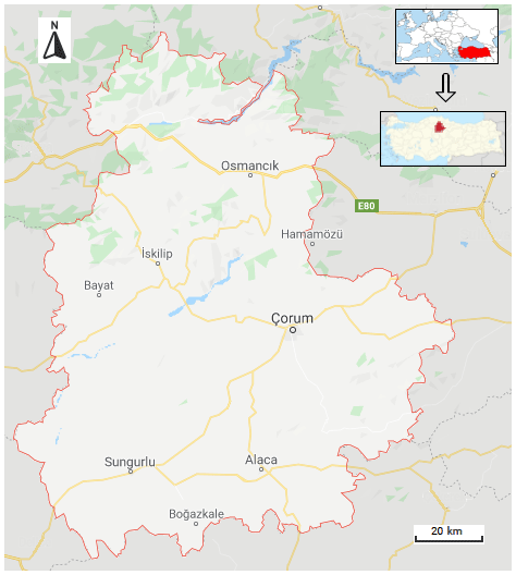
Figure 1Location of the study area, Corum Province, Turkey (© Google Maps).
Table 1Basic statistics of the data used in the study during the training and testing periods.

NB: T: temperature, n: sunshine duration, U: wind speed, RH: relative humidity.
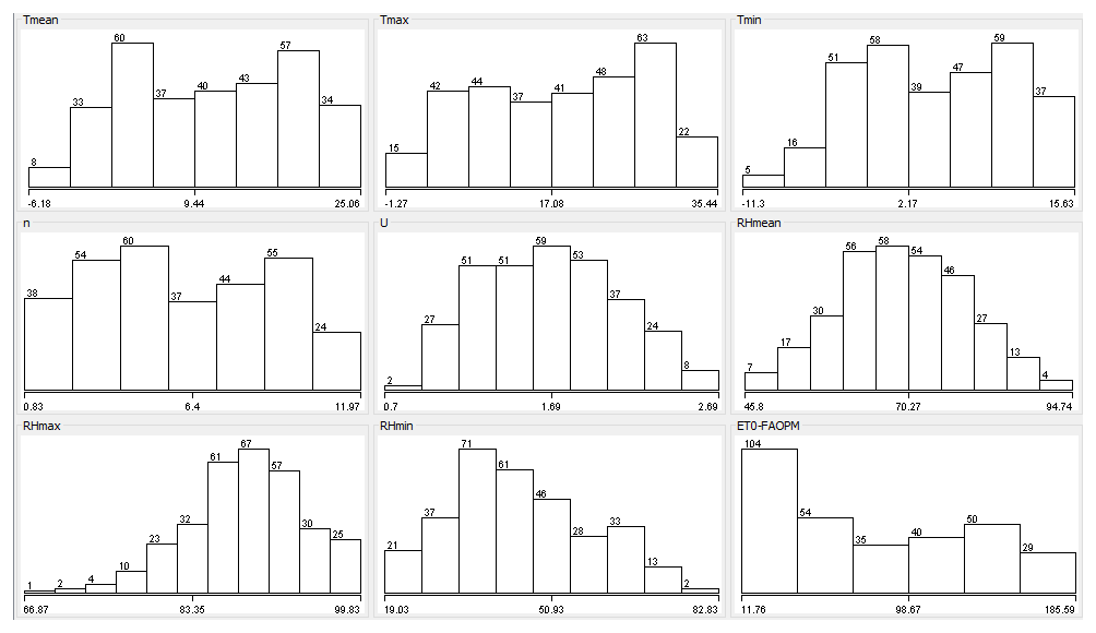
Figure 2Frequency distributions of meteorological input dataset conforming to the distribution statistics.
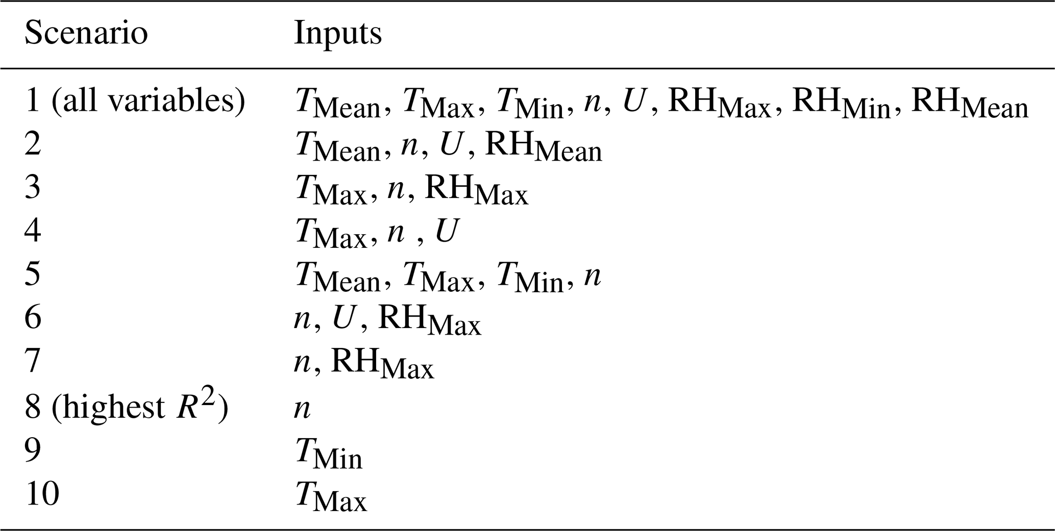
To determine the meteorological factors employed in the model and the formation of scenarios, the relationships between ET0 and other variables were calculated as given in Fig. 3. Input determination is an essential component of model development as irrelevant inputs are likely to worsen the model performances (Hejazi and Cai, 2009; Maier and Dandy, 2000; Maier et al., 2010), while a set of carefully selected inputs could ease the model training process and increase the physical representation whilst providing a better understanding of the system (Bowden et al., 2005). The sunshine duration in this study was very highly correlated with ET0 (R2=0.92), and the variables Tmean, Tmax, and Tmin were all highly correlated (R2>0.8). The RH mean was the least correlated variable (R2=0.24) in this study. As can be understood visually, the meteorological variables associated with temperature and especially the sunshine duration have a high correlation with ET0. Considering these relationships, 10 different input scenarios were created, and the effect of meteorological variables on ET0 estimation was evaluated. Table 2 gives the meteorological variables used in each scenario. While all parameters were taken into account in the first scenario, the ones that could affect ET0 more in the following scenarios were added in the respective scenarios.

Figure 3Scatter plot showing the correlation between ET0 and the independent variable. The coefficient of determination has been added for clarity.
Table 2The scenarios developed in this study with respective inputs in respective scenarios.
3.1 Calculation of ET0
The United Nations Food and Agriculture Organization (FAO) recommend the Penman–Monteith (PM) equation (Eq. 1) to calculate the evapotranspiration of reference crops (Doorenbos and Pruitt, 1977). Although the PM equation is much more complex than the other equations, it has been formally explained by FAO. The equation has two main features: (1) it can be used in any weather conditions without local calibration, and (2) the performance of the equation is based on the lysimetric data in an approved spherical range (Allen et al., 1989). The requirement for many meteorological factors can be defined as the main problem. However, there is still no equipment to record these parameters correctly in many countries, or data are not regularly recorded (Gavili et al., 2018).
where ET0 refers to the reference evapotranspiration [mm d−1], G refers to the soil heat flux density [MJ m−2 d−1], u2 refers to the wind speed at 2 m [m s−1], ea refers to the actual vapour pressure [kPa], es refers to the saturation vapour pressure [kPa], es−ea refers to the saturation vapour pressure deficit [kPa], T refers to the mean daily air temperature at 2 m [∘C], Rn refers to the net radiation at the crop surface [MJ m−2 d−1], γ refers to the psychrometric constant [kPa ∘C−1], and Δ refers to the slope vapour pressure curve [kPa ∘C−1].
3.2 Broyden–Fletcher–Goldfarb–Shanno artificial neural network (BFGS-ANN)
McCulloch and Pitts (1943) pioneered the original idea of neural networks. ANN is essentially a black-box modelling approach that does not identify the training algorithm explicitly, yet the modellers often trial several algorithms to attain an optimal model (Deo and Şahin, 2015). In this study, the Broyden–Fletcher–Goldfarb–Shanno (BFGS) training algorithm has been used to estimate ET0 amounts. In optimization studies, the BFGS method is a repetitious approach for solving unlimited nonlinear optimization problems (Fletcher, 1987). The BFGS-ANN technique trains a multilayer perceptron ANN with one hidden layer by reducing the given cost function plus a quadratic penalty using the BFGS technique. The BFGS approach includes quasi-Newtonian methods. For such problems, the required condition for reaching an optimal level occurs when the gradient is zero. Newtonian and the BFGS methods cannot be guaranteed to converge unless the function has a quadratic Taylor expansion near an optimum. However, BFGS can have a high accuracy even for non-smooth optimization instances (Curtis and Que, 2015).
Quasi-Newtonian methods do not compute the Hessian matrix of second derivatives. Instead, the Hessian matrix is drawn by updates specified by gradient evaluations. Quasi-Newtonian methods are extensions of the secant method to reach the basis of the first derivative for multi-dimensional problems. The secant equation does not specify a specific solution in multi-dimensional problems, and quasi-Newtonian methods differ in limiting the solution. The BFGS method is one of the frequently used members of this class (Nocedal and Wright, 2006). In the BFGS-ANN method application, all attributes, including the target attribute (meteorological variables and ET0), are standardized. In the output layer, the sigmoid function is employed for classification. In approximation, the sigmoidal function can be specified for both hidden and output layers. For regression, the activation function can be employed as the identity function in the output layer. This method was implemented on the basis of radial basis function networks trained in a fully supervised manner using Weka's optimization class by minimizing squared error with the BFGS method. In this method, all attributes are normalized into the [0, 1] scale (Frank, 2014).
3.3 Support vector regression (SVR)
The statistical learning theory is the basis of the SVM. The optimum hyperplane theory and kernel functions and nonlinear classifiers were added as linear classifiers (Vapnik, 2013). Models of the SVM are separated into two main categories: (a) the classifier SVM and (b) the regression (SVR) model. An SVM is employed to classify data in various classes, and the SVR is employed for estimation problems. Regression is used to take a hyperplane suitable for the data used. The distance to any point in this hyperplane shows the error of that point. The best technique proposed for linear regression is the least-squares (LS) method. However, it may be entirely impossible to use the LS estimator in the presence of outliers. In this case, a robust predictor has to be developed that will not be sensitive to minor changes, as the processor will perform poorly. Three kernel functions were used including the polynomial, Pearson VII function-based universal, and radial basis function with the level of Gaussian noise parameters added to the diagonal of the covariance matrix and the random number of seed to be used (equal to 1.0); the most suitable kernel function in each scenario was determined by trial and error (Frank, 2014), and the description of kernels is provided in Sect. 3.6.
3.4 Gaussian process regression (GPR)
The GPR or GP is defined by Rasmussen and Williams (2005) as a complex set of random variables, which have a joint Gaussian distribution. Kernel-based methods such as SVM and GPs can work together to solve flexible and applicable problems. The GP is generally explained by two functions: average and covariance functions (Eq. 2). The average function is a vector; the covariance function is a matrix. The GP model is possibly a nonparametric black box technique.
where f refers to Gaussian distribution, m refers to a mean function, and k refers to covariance function.
The value of covariance expresses the correlation between the individual outputs concerning the inputs. The covariance value determines the correlation between individual outputs and inputs. The covariance function produces a matrix of two parts (Eq. 3).
Here, Cf represents the functional part but defines the unknown part of the modelling system, while Cn represents the system's noise part. A Gaussian process (GP) is closely related to SVM, and both are part of the kernel machine area in ML models. Kernel methods are sample-based learners. Instead of learning a fixed parameter, the kernels memorize the training data sample and assign a certain weight to it.
3.5 Long short-term memory (LSTM)
LSTM is a high-quality evolution of recurrent neural networks (RNNs). This neural network is presented to address the problems that existed in RNNs by adding more interactions per cell. The LSTM system is also special since it remembers information for an extended period. Moreover, LSTM consists of four essential interacting layers, which have different communication methods.
The next thing is that its complete network consists of a memory block. These blocks are also called cells. The information is stored in one cell and then transferred into the next one with the help of gate controls. Through the help of these gates, it becomes straightforward to analyse the information accurately. All of these gates are extremely important, and they are called forget gates as explained in Eq. (4).
LSTM units or blocks are part of the repetitive neural network structure. Repetitive neural networks are made to use some artificial memory processes that can help these AI algorithms to mimic human thinking.
3.6 Kernel functions
Four different kernel functions are frequently used as depicted in the literature including the polynomial, radial-based function, Pearson VII function (PUK), and normalized polynomial kernels, and their formulas and parameters are tabulated in Table 3. As is clear from Table 3, some parameters must be determined by the user for each kernel function. While the number of parameters to be determined for a PUK kernel is two, it requires determining a parameter in the model formation that will be the basis for classification for other functions. When kernel functions are compared, it is seen that polynomial- and radial-based kernels are more plain and understandable. Although it may seem mathematically simple, the increase in the degree of the polynomial makes the algorithm complex. This significantly increases processing time and decreases the classification accuracy after a point. In contrast, changes in the radial-based function parameter (γ), expressed as the kernel size, were less effective on classification performance (Hsu et al., 2010). The normalized polynomial function was proposed by Graf and Borer (2001) in order to normalize the mathematical expression of the polynomial kernel instead of normalizing the dataset.
Table 3Basic kernel functions used in the study with parameters that needed to be determined.

The normalized polynomial kernel is a generalized version of the polynomial kernel. On the other hand, the PUK kernel has a more complex mathematical structure than other kernel functions with its two parameters (σ, ω) known as Pearson width. These two parameters affect classification accuracy and these parameters are not known in advance. For this reason, determining the most suitable parameter pair in the use of the PUK kernel is an important step.
The user must determine the editing parameter C for all SVMs during runtime. If values that are too small or too large for this parameter are selected, the optimum hyperplane cannot be determined correctly. Therefore there will be a serious decrease in classification accuracy. On the other hand, if C is equal to infinity, the SVM model becomes suitable only for datasets that can be separated linearly. As can be seen from here, the selection of appropriate values for the parameters directly affects the accuracy of the SVM classifier. Although a trial-and-error strategy is generally used, the cross-validation approach enables successful results. The purpose of the cross-validation approach is to determine the performance of the classification model created. For this purpose, the data are separated into two categories, where the first is used to train the model and the second part is processed as test data to determine the model's performance. As a result of applying the model created with the training set to the test dataset, the number of samples classified correctly indicates the classifier's performance. Therefore, by using the cross-validation method, the classification and determination of the best kernel parameters were obtained (Kavzoglu and Golkesen, 2010).
In this study, during SVR and GPR modelling, the three kernel functions as in Table 3 were used, and the most suitable kernel function in each scenario was determined by trial and error (Frank, 2014). For the BFGS-ANN, SVR, and GPR methods in the Weka software were used, while Python language was used for the LSTM method.
3.7 Model evaluation
The statistical parameters used in the selection and comparison of the models in the study included the root mean square error (RMSE), mean absolute error (MAE), and correlation fit (R) as shown in Eqs. (5)–(7). Here, Xi and Yi are the observed and predicted values, and N is the number of data.
In addition, Taylor diagrams were prepared to check the performance of the models, which illustrates the experimental and statistical parameters simultaneously.
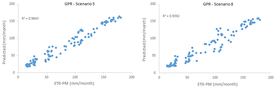
Figure 4Scatter plots comparing GPR-estimated and FAO56PM-estimated ET0 in scenarios 5 and 8.

Figure 5Time series graphics of GPR-estimated and FAO56PM-estimated ET0 in scenarios 5 and 8.
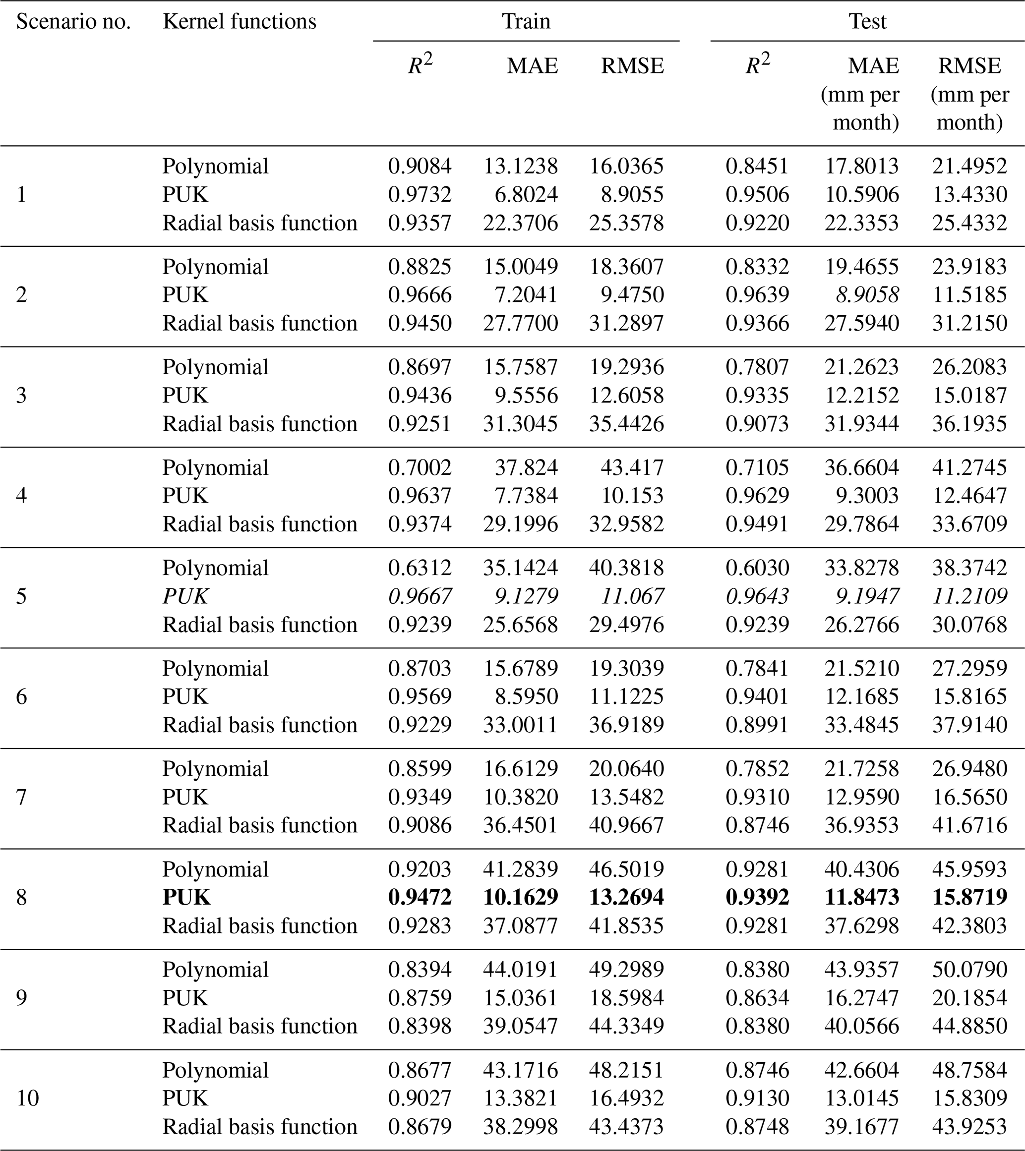
In this study, 10 different scenarios were created by using combinations of input variables, i.e. monthly average; highest and lowest temperature; sunshine duration; wind speed; and average, highest, and lowest relative humidity data. ET0 amounts were estimated with the help of kernel-based GPR and SVR methods, a BFGS-ANN, and one of the deep learning LSTM models. ET0 estimation results obtained from different scenarios according to the GPR method are summarized in Table 4. As can be seen from the table, scenario 5, with the GPR method PUK function, contains four meteorological variables including TMax, TMin, TMean, and n and gave the best result (training period: R2=0.9667, MAE = 9.1279 mm per month, RMSE = 11.067 mm per month; testing period: R2=0.9643, MAE = 9.1947 mm per month, RMSE = 11.2109 mm per month). However, scenario 8, with only one meteorological variable (sunshine duration), registered quite good results for the training period (R2=0.9472, MAE = 10.1629 mm per month, RMSE = 13.2694 mm per month) and testing period (R2=0.9392, MAE = 11.8473 mm per month, RMSE = 15.8719 mm per month). Since the scenario with the fewest input parameters and with an acceptable level of accuracy is largely preferred, scenario 8 was chosen as the optimum scenario.
Table 4Outcomes of the GPR modelling approach from different kernel functions based on R2, MAE, and RMSE (italic font represents the best results; bold represents the optimally selected model).
The scatter plot and time series plots of the test phase for scenarios 5 and 8 are given in Figs. 4 and 5. As can be seen from these figures, a relative agreement has been achieved between the FAO56PM ET0 values and the ET0 values modelled. When the time series graphs are examined, minimum points in estimated ET0 values are more in harmony with FAO56PM values than maximum points.
For the SVR model, again three different kernel functions were evaluated in respective scenarios under the same conditions, and the results are displayed in Table 5. As can be seen here, scenarios 5 and 8 have yielded the best and most appropriate results according to the PUK function. The results of scenario 5 with TMean, TMin, TMax, and n as input variables gave the best result (training period: R2=0.9838, MAE = 6.0500 mm per month, RMSE = 8.5733 mm per month; testing period: R2=0.9771, MAE = 7.07 mm per month, RMSE = 9.3259 mm per month). However, scenario 8 gave the most appropriate result (training period: R2=0.9398, MAE = 9.7984 mm per month, RMSE = 13.0830 mm per month; testing period: R2=0.9392, MAE = 11.2408 mm per month, RMSE = 15.5611 mm per month) with only one meteorological input variable, i.e. the sunshine duration (n). Although the accuracy rate of scenario 8 is somewhat lower than scenario 5, it provides convenience and is preferred in terms of application and calculation since it requires a single input. The sunshine duration can be measured easily and without the need for high-cost equipment and personnel. Consequently, by using only one parameter, the amount of ET0 is estimated within acceptable accuracy limits.

Figure 6Scatter plots comparing SVR-estimated and FAO56PM-estimated ET0 in scenarios 5 and 8.
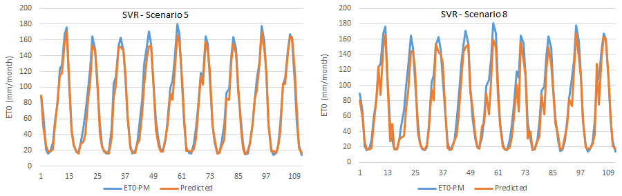
Figure 7Time series graphics of SVR-estimated and FAO56PM-estimated ET0 in scenarios 5 and 8.
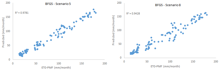
Figure 8Scatter plots comparing BFGS-ANN-estimated and FAO56PM-estimated ET0 in scenarios 5 and 8.
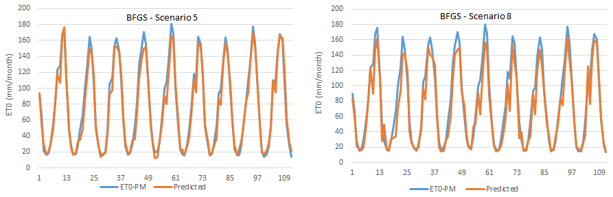
Figure 9Time series graphics of BFGS-ANN-estimated and FAO56PM-estimated ET0 in scenarios 5 and 8.
Table 5Outcomes of the SVR modelling approach from different kernel functions based on R2, MAE, and RMSE (italic font represents the best results; bold represents the optimally selected model).
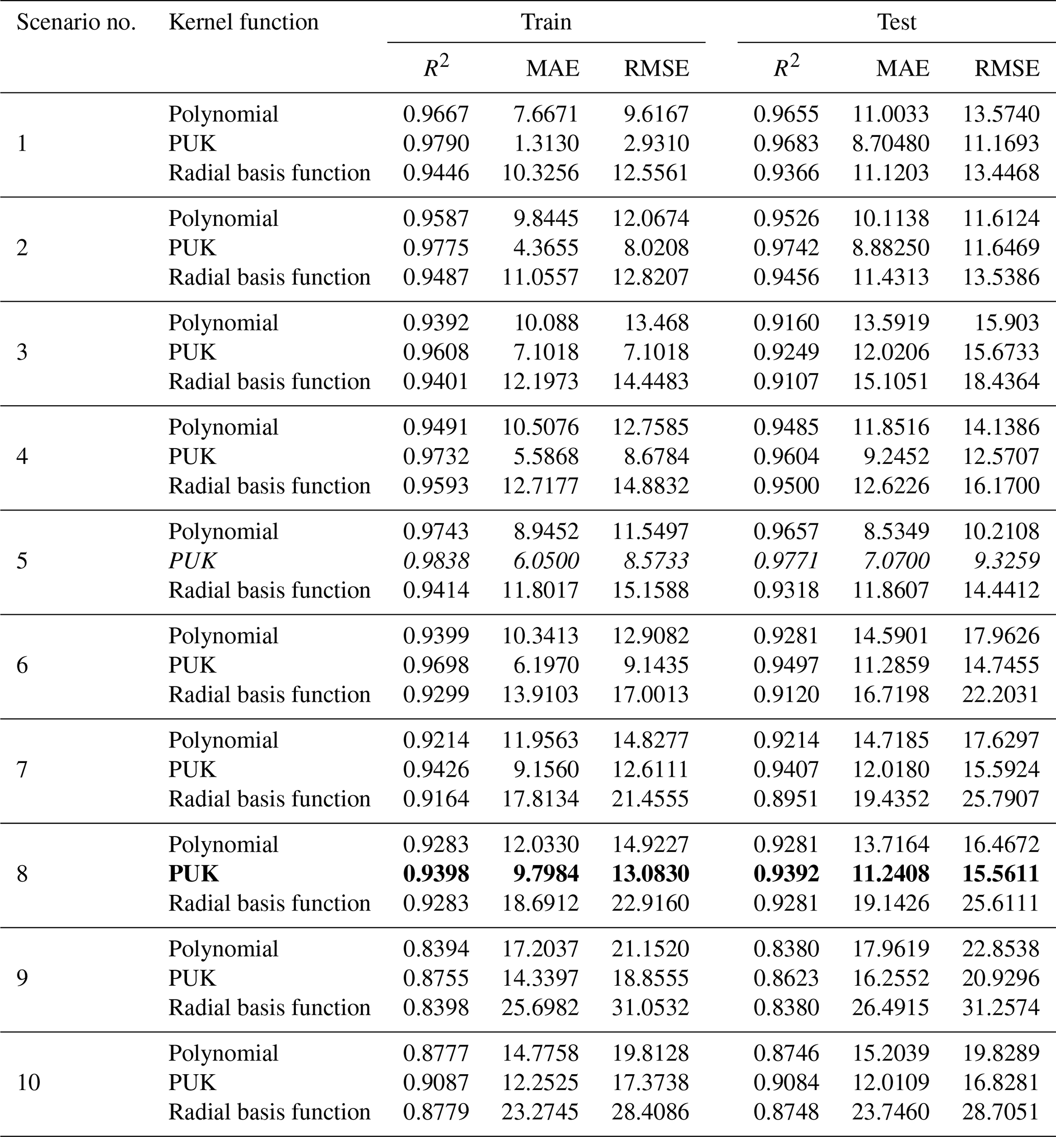
The scatter plot and time series graph drawn for the SVR model are given in Figs. 6 and 7, which shows that all points are compatible with FAO56PM ET0 values and ET0 values estimated from the model, except for the less frequent endpoints. The R2 values were also very high (R2>0.939).
In this study, the BFGS training algorithm was specifically used to train the ANN architecture, and ET0 amounts were estimated for all scenarios. The results are given in Table 6. In implementing the BFGS-ANN method, all features, including the target feature (meteorological variables and ET0) are standardized. In the hidden and output layer, the sigmoid function is ) used for classification.
Table 6Outcomes of the BFGS-ANN modelling approach for different scenarios based on R2, MAE, and RMSE (italic font represents the best results; bold represents the optimally selected model).

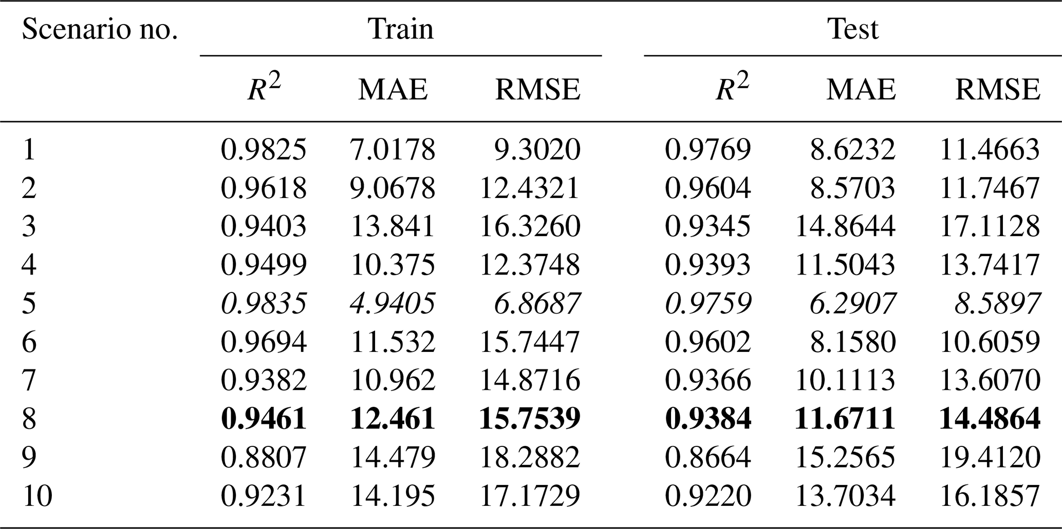
Table 7Outcomes of the LSTM modelling approach for different scenarios based on R2, MAE, and RMSE (italic font represents the best results; bold represents the optimally selected model).
As can be seen here, scenarios 5 and 8 gave the best and most relevant results. According to the results, scenario 5 including TMean, TMin, TMax, and n meteorological variables again produced the best result (training period: R2=0.9843, MAE = 8.0025 mm per month, RMSE = 9.9407 mm per month; testing period: R2=0.9781, MAE = 6.7885 mm per month RMSE = 8.8991 mm per month). However, scenario 8 gave the most appropriate result (training period: R2=0.9474, MAE = 10.1139 mm per month, RMSE = 13.1608 mm per month; testing period: R2=0.9428, MAE = 11.4761 mm per month, RMSE = 15.6399 mm per month) with only the sunshine duration (n) as a meteorological input variable, and hence it is selected as the optimal BFGS-ANN model. Although scenario 8's accuracy rate is marginally lower than that of scenario 5, it is easy and practical in terms of application and calculation since it consists of only one parameter. The scatter plot and time series graph drawn for the BFGS-ANN model, given in Figs. 8 and 9, concurs with the statistical metrics of Table 6. As can be seen, the BFGS-ANN method predicted ET0 amounts with a high success rate, and a high level of agreement was achieved between the estimates obtained from the model and FAO56PM ET0 values. The R2 values were also very high (R2>0.942).
Finally, the LSTM method, which is a deep learning technique, was used to estimate the ET0 under the same 10 scenarios. Two hidden layers with 200 and 150 neurons were utilized in LSTM with the rectified linear unit (ReLU) activation function and Adam optimizations. The other parameters, learning rate alternatives from to , decay as to , and 500–750–1000 as epochs, have been tried. The best results obtained for 10 different scenarios at the modelling stage, according to the LSTM method, are given in Table 7.
Table 8Statistical values of the test phase for selected scenarios (the best/closest results are in bold).
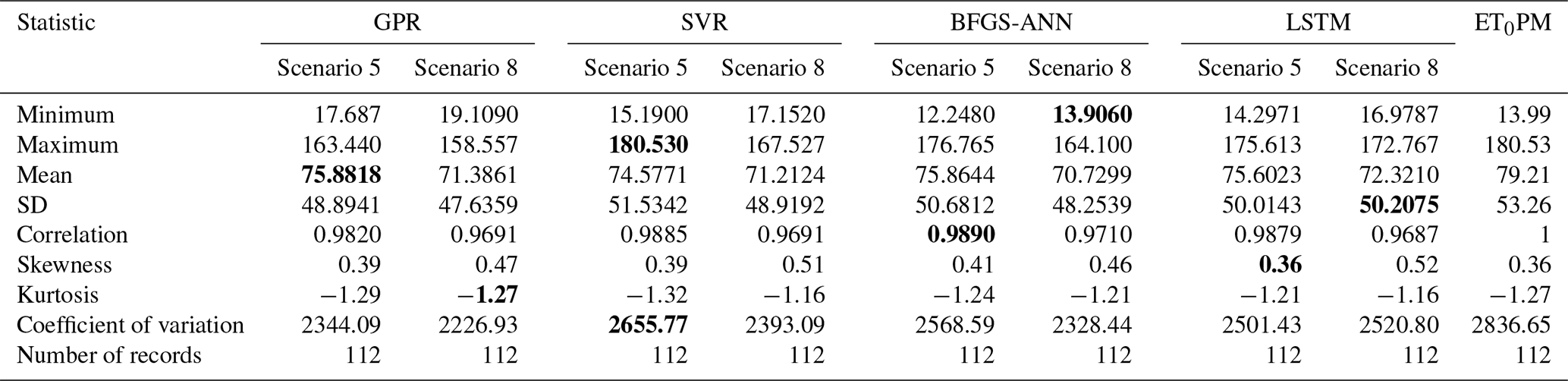
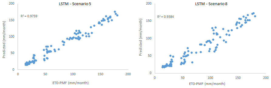
Figure 10Scatter plots comparing LSTM-estimated and FAO56PM-estimated ET0 in scenarios 5 and 8.
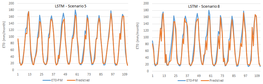
Figure 11Time series graphics of LSTM-estimated and FAO56PM-estimated ET0 in scenarios 5 and 8.
As in other methods, scenarios 5 and 8 of the LSTM model registered the best and most appropriate results. In scenario 5 TMean, TMin, TMax, and n as the input variables gave the best result (training period: R2=0.9835, MAE = 4.9405 mm per month, RMSE = 6.8687 mm per month; testing period: R2=0.9759, MAE = 6.2907 mm per month RMSE = 8.5897 mm per month). However, scenario 8 gave the most appropriate result (training period: R2=0.9461, MAE = 12.461 mm per month, RMSE = 15.7539 mm per month; testing period: R2=0.9384, MAE = 11.6711 mm per month, RMSE = 14.4864 mm per month) with the sunshine duration (n) meteorological variable as the input to the model.
Scatter plot and time-series graphs of observed and LSTM-predicted ET0 are given in Figs. 10 and 11, where again a high success rate and a high level of agreement were achieved between the estimates obtained from the model and FAO56PM ET0 values.
In order to compare and evaluate the models used in this study, statistical values for the test phase are given in both FAO56PM ET0 and the respective models in Table 8. The lowest skewness coefficient of 0.39 was found in scenario 5 in both GPR and SVR methods and the highest of 0.52 in LSTM scenario 8. Tmean has the lowest kurtosis coefficient of −1.23 and RHmean has the highest of 0.36. The highest variation was observed in RHmin with 174.19 and the lowest in U with 0.17.
As can be seen from Table 8, the closest value to the FAO56PM ET0 minimum value (13.99 mm per month) is scenario 8 in the BFGS-ANN method (13.906 mm per month). Furthermore, the FAO56PM ET0 maximum value (180.53 mm per month) has been reached in scenario 5 (180.53 mm per month) in the SVR method, which is the closest and even the same value. The value closest to the mean value of FAO56PM ET0 (79.21 mm per month) corresponds to scenario 5 (75.8818 mm per month) in the GPR method; the value closest to the FAO56PM ET0 SD value (53.26 mm per month) is the value of scenario 5 (51.5342 mm per month) in the SVR method. As shown in Table 8, all methods have estimated the ET0 amounts within acceptable levels, yet disparate results are attained when comparing the statistics. Having said that, when models are ranked according to the correlation coefficient, the best results were BFGS-ANN, SVR, LSTM, and GPR in scenario 5 and BFGS-ANN, GPR, SVR, and LSTM in scenario 8.
Furthermore, to have precise model comparative evaluations besides the tables, the Taylor diagram for the scenarios 5 and 8 were plotted as in Fig. 12. The points on the polar Taylor graph are used to study the adaption between measured and predicted values in the Taylor diagram. The correlation coefficient and normalized standard deviation are also indicated by the azimuth angle and radial distances from the base point, respectively (Taylor, 2001). As displayed in the figure, all four models performed quite well but the BFGS-ANN seemed to achieve higher success than others. As seen in the Fig. 1 histogram, FAO56PM ET0 values do not conform to normal distribution. This mismatch is considered to be the reason for the poor performances of the GPR method over comparative models.
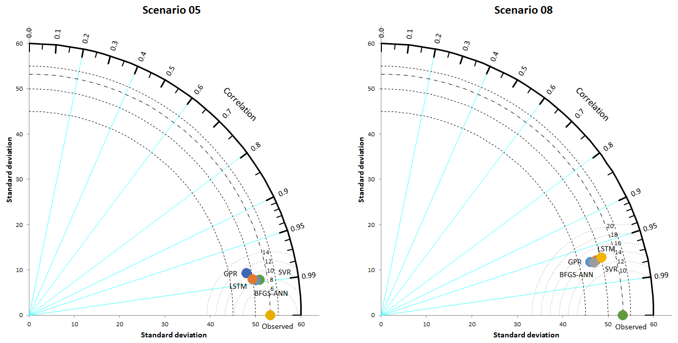
The results of Fig. 12 also show that model performances were higher in scenario 5; however, using the fewest input parameters to develop the most parsimonious model was the key target of the study and was achieved by scenario 8, in which ET0 values were estimated correctly at relatively appropriate and acceptable levels. Therefore, these methods produced trustworthy results and have the potential to make correct estimations in climates similar to the study area.
The amount of ET0 can be calculated with many empirical equations. However, these equations can generally differ spatially and require the knowledge of many parameters. Since ET0 includes a complex and nonlinear structure, it cannot be easily estimated with the previously measured data without requiring numerous parameters. In this study, estimating the ET0 with different machine learning and deep learning methods was made using the fewest meteorological variables in Turkey's Corum region, which has an arid and semi-arid climate and is regarded as a strategic agricultural region. In this context, firstly, ET0 amounts were calculated with the Penman–Monteith method and taken as the output of the models. Then, 10 different scenarios were created using different combinations of meteorological variables. Consequently, kernel-based GPR and SVR methods and BFGS-ANN and LSTM models were developed for monthly ET0 amount estimations. The results revealed better performance of the BFGS-ANN model in comparison to other models in this study, although all four methods predicted ET0 amounts within acceptable accuracy and error levels. In kernel-based methods (GPR and SVR), PUK was the most successful kernel function. Scenario 5, which is related to temperature and includes four meteorological variables (mean temperature, highest and lowest temperature averages, and sunshine duration), gave the best results in all the scenarios used. Scenario 8, which included only the sunshine duration, was determined as the most suitable and parsimonious scenario. In this case, the ET0 amount was estimated using only sunshine duration without the need for other meteorological parameters for the study area. The Corum region is described as arid and semi-arid with low rainfall and cloudiness and longer sunshine duration; hence sunshine hours are the key driving factor of ET0 in the region, which is clearly highlighted by high model performances with sunshine hours as the only input. Continuous measurement of meteorological variables in large farmland areas is a costly process that requires expert personnel, time, or good equipment. Simultaneously, some equations used for ET0 calculations are not preferred by specialists because they contain many parameters. In this case, it is very advantageous for water resources managers to estimate ET0 amounts only with sunshine duration time, which is easy to measure and requires no extra cost. A follow-up study aims to evaluate the performance of GPR and LSTM models in a larger area on a daily timescale and with data to be obtained from more meteorology stations.
Code is available on request due to privacy or other restrictions.
Data are available on request due to privacy or other restrictions.
The conceptualization of the paper was performed by MTS and HA. Data curation was done by MTS and HA. MTS and HA also acquired the funding for this study. The project was investigated by MTS, HA, and MTS, who also developed the methodology. Project administration was handled by HA. Software development was carried out by MTS, AM, and HA. Validation was performed by AM and SSB. The writing of original draft was handled by MTS, HA, and SSB, while all authors (MTS, HA, SSB, and RP) handled the visualization and the writing, reviewing, and editing of the paper. All authors have read and agreed to the published version of the paper.
The authors declare that they have no conflict of interest.
This research has been supported by the The Scientific and Technological Research Council of Turkey (grant no. 1059B211900014) and the Open Access Funding by the Publication Fund of the TU Dresden.
This paper was edited by Dimitri Solomatine and reviewed by Hatice Çıtakoğlu and one anonymous referee.
Abrishami, N., Sepaskhah, A. R., and Shahrokhnia, M. H.: Estimating wheat and maize daily evapotranspiration using artificial neural network, Theor. Appl. Climatol., 135, 945–958, https://doi.org/10.1007/s00704-018-2418-4, 2019.
Allen, R. G., Jensen, M. E., Wright, J. L., and Burman, R. D.: Operational Estimates of Reference Evapotranspiration, Agron. J., 81, 650–662, https://doi.org/10.2134/agronj1989.00021962008100040019x, 1989.
Anli, A. S.: Temporal Variation of Reference Evapotranspiration (ET0) in Southeastern Anatolia Region and Meteorological Drought Analysis through RDI (Reconnaissance Drought Index) Method, J. Agric. Sci. Tarim Bilim. Derg., 20, 248–260, https://doi.org/10.15832/tbd.82527, 2014.
Bowden, G. J., Dandy, G. C., and Maier, H. R.: Input determination for neural network models in water resources applications. Part 1 – background and methodology, J. Hydrol., 301, 75–92, https://doi.org/10.1016/j.jhydrol.2004.06.021, 2005.
Citakoglu, H., Cobaner, M., Haktanir, T., and Kisi, O.: Estimation of Monthly Mean Reference Evapotranspiration in Turkey, Water Resour. Manage., 28, 99–113, https://doi.org/10.1007/s11269-013-0474-1, 2014.
Cobaner, M., Citakoğlu, H., Haktanir, T., and Kisi, O.: Modifying Hargreaves–Samani equation with meteorological variables for estimation of reference evapotranspiration in Turkey, Hydrol. Res., 48, 480–497, https://doi.org/10.2166/nh.2016.217, 2017.
Curtis, F. E. and Que, X.: A quasi-Newton algorithm for nonconvex, nonsmooth optimization with global convergence guarantees, Math. Program. Comput., 7, 399–428, https://doi.org/10.1007/s12532-015-0086-2, 2015.
Deo, R. C. and Şahin, M.: Application of the Artificial Neural Network model for prediction of monthly Standardized Precipitation and Evapotranspiration Index using hydrometeorological parameters and climate indices in eastern Australia, Atmos. Res., 161–162, 65–81, https://doi.org/10.1016/j.atmosres.2015.03.018, 2015.
Doorenbos, J. and Pruitt, W. O.: Crop Water Requirements, FAO Irrigation and Drainage Paper 24, FAO, Rome, p. 144, 1977.
Feng, Y., Cui, N., Zhao, L., Hu, X., and Gong, D.: Comparison of ELM, GANN, WNN and empirical models for estimating reference evapotranspiration in humid region of Southwest China, J. Hydrol., 536, 376–383, https://doi.org/10.1016/j.jhydrol.2016.02.053, 2016.
Fletcher, R.: Practical methods of optimization, 2nd Edn., John Wiley & Sons, New York, ISBN 978-0-471-91547-8, 1987.
Frank, E.: Fully supervised training of Gaussian radial basis function networks in WEKA, Computer Science Working Papers 04/2014, Department of Computer Science, The University of Waikato, Hamilton, NZ, 2014.
Gavili, S., Sanikhani, H., Kisi, O., and Mahmoudi, M. H.: Evaluation of several soft computing methods in monthly evapotranspiration modelling, Meteorol. Appl., 25, 128–138, https://doi.org/10.1002/met.1676, 2018.
Graf, A. B. A. and Borer, S.: Normalization in Support Vector Machines, Lect. Note. Comput. Sci., 2191, 277–282, 2001.
Hargreaves, G. H. and Samani, Z. A.: Reference Crop Evapotranspiration from Temperature, Appl. Eng. Agric., 1, 96–99, https://doi.org/10.13031/2013.26773, 1985.
Hejazi, M. I. and Cai, X.: Input variable selection for water resources systems using a modified minimum redundancy maximum relevance (mMRMR) algorithm, Adv. Water Resour., 32, 582–593, https://doi.org/10.1016/j.advwatres.2009.01.009, 2009.
Hsu, C. W., Chang, C. C., and Lin, C. J.: A Practical Guide to Support Vector Classification, available at: http://www.csie.ntu.edu.tw/~cjlin/papers/guide/guide.pdf (last access: 25 December 2020), 2010.
Kavzoglu, T. and Colkesen, I.: Investigation of the Effects of Kernel Functions in Satellite Image Classification Using Support Vector Machines, Harita Dergisi Temmuz 2010 Sayi 144, General Directorate of Mapping, Ankara, Turkey, 2010.
Koch, J., Berger, H., Henriksen, H. J., and Sonnenborg, T. O.: Modelling of the shallow water table at high spatial resolution using random forests, Hydrol. Earth Syst. Sci., 23, 4603–4619, https://doi.org/10.5194/hess-23-4603-2019, 2019.
Maier, H. R. and Dandy, G. C.: Neural networks for the prediction and forecasting of water resources variables: a review of modelling issues and applications, Environ. Model. Softw., 15, 101–124, https://doi.org/10.1016/S1364-8152(99)00007-9, 2000.
Maier, H. R., Jain, A., Dandy, G. C., and Sudheer, K. P.: Methods used for the development of neural networks for the prediction of water resource variables in river systems: Current status and future directions, Environ. Model. Softw., 25, 891–909, https://doi.org/10.1016/j.envsoft.2010.02.003, 2010.
McCulloch, W. S. and Pitts, W.: A logical calculus of the ideas immanent in nervous activity, Bull. Math. Biophys., 5, 115–133, https://doi.org/10.1007/BF02478259, 1943.
Nema, M. K., Khare, D., and Chandniha, S. K.: Application of artificial intelligence to estimate the reference evapotranspiration in sub-humid Doon valley, Appl. Water Sci., 7, 3903–3910, https://doi.org/10.1007/s13201-017-0543-3, 2017.
Nocedal, J. and Wright, S.: Numerical Optimization, Springer, New York, 2006.
Pandey, P. K., Nyori, T., and Pandey, V.: Estimation of reference evapotranspiration using data driven techniques under limited data conditions, Model. Earth Syst. Environ., 3, 1449–1461, https://doi.org/10.1007/s40808-017-0367-z, 2017.
Pereira, L. S., Perrier, A., Allen, R. G., and Alves, I.: Evapotranspiration: Concepts and Future Trends, J. Irrig. Drain. Eng., 125, 45–51, https://doi.org/10.1061/(ASCE)0733-9437(1999)125:2(45), 1999.
Prasad, R., Deo, R. C., Li, Y., and Maraseni, T.: Input selection and performance optimization of ANN-based streamflow forecasts in the drought-prone Murray Darling Basin region using IIS and MODWT algorithm, Atmos. Res., 197, 42–63, https://doi.org/10.1016/j.atmosres.2017.06.014, 2017.
Prasad, R., Joseph, L., and Deo, R. C.: Modeling and Forecasting Renewable Energy Resources for Sustainable Power Generation: Basic Concepts and Predictive Model Results, in: Translating the Paris Agreement into Action in the Pacific, Springer, Cham, Zug, Switzerland, 59–79, 2020.
Quej, V. H., Almorox, J., Arnaldo, J. A., and Saito, L.: ANFIS, SVM and ANN soft-computing techniques to estimate daily global solar radiation in a warm sub-humid environment, J. Atmos. Sol.-Terr. Phy., 155, 62–70, https://doi.org/10.1016/j.jastp.2017.02.002, 2017.
Rana, G. and Katerji, N.: Measurement and estimation of actual evapotranspiration in the field under Mediterranean climate: a review, Eur. J. Agron., 13, 125–153, https://doi.org/10.1016/S1161-0301(00)00070-8, 2000.
Rasmussen, C. E. and Williams, C. K. I.: Gaussian Processes for Machine Learning, in: Adaptive Computation and Machine Learning series, MIT Press, Cambridge, Massachusetts, ISBN 0-262-18253-X, 2005.
Reis, M. M., da Silva, A. J., Zullo Junior, J., Tuffi Santos, L. D., Azevedo, A. M., and Lopes, É. M. G.: Empirical and learning machine approaches to estimating reference evapotranspiration based on temperature data, Comput. Electron. Agric., 165, 104937, https://doi.org/10.1016/j.compag.2019.104937, 2019.
Republic of Turkey: Agricultural data of Corum province, Corum province Food Agriculture Livestock Directorate, Corum, Ministry of Agriculture and Forestry, 2017.
Saggi, M. K. and Jain, S.: Reference evapotranspiration estimation and modelling of the Punjab Northern India using deep learning, Comput. Electron. Agric., 156, 387–398, https://doi.org/10.1016/j.compag.2018.11.031, 2019.
Sattari, M. T., Pal, M., Yürekli, K., and Ünlükara, A.: M5 model trees and neural network based modelling of ET0 in Ankara, Turkey, Turk. J. Eng. Environ. Sci., 37, 211–219, https://doi.org/10.3906/muh-1212-5, 2013.
Shabani, S., Samadianfard, S., Sattari, M. T., Mosavi, A., Shamshirband, S., Kmet, T., and Várkonyi-Kóczy, A. R.: Modeling Pan Evaporation Using Gaussian Process Regression K-Nearest Neighbors Random Forest and Support Vector Machines; Comparative Analysis, Atmosphere (Basel), 11, 66, https://doi.org/10.3390/atmos11010066, 2020.
Shamshirband, S., Amirmojahedi, M., Gocić, M., Akib, S., Petković, D., Piri, J., and Trajkovic, S.: Estimation of Reference Evapotranspiration Using Neural Networks and Cuckoo Search Algorithm, J. Irrig. Drain. Eng., 142, 04015044, https://doi.org/10.1061/(ASCE)IR.1943-4774.0000949, 2016.
Solomatine, D. P.: Applications of data-driven modelling and machine learning in control of water resources, in: Computational intelligence in Control, edited by: Mohammadian, M., Sarker, R. A., and Yao, X., Idea Group Publishing, Pennsylvania, 197–217, 2002.
Solomatine, D. P. and Dulal, K. N.: Model trees as an alternative to neural networks in rainfall–runoff modelling, Hydrolog. Sci. J., 48, 399–411, https://doi.org/10.1623/hysj.48.3.399.45291, 2003.
Taylor, K. E.: Summarizing multiple aspects of model performance in a single diagram, J. Geophys. Res.-Atmos., 106, 7183–7192, https://doi.org/10.1029/2000JD900719, 2001.
Vapnik, V.: The Nature of Statistical Learning Theory, Springer Science & Business Media, Berlin, Germany, 2013.
Wen, X., Si, J., He, Z., Wu, J., Shao, H., and Yu, H.: Support-Vector-Machine-Based Models for Modeling Daily Reference Evapotranspiration With Limited Climatic Data in Extreme Arid Regions, Water Resour. Manage., 29, 3195–3209, https://doi.org/10.1007/s11269-015-0990-2, 2015.
Xu, C.-Y. and Singh, V. P.: Evaluation and generalization of temperature-based methods for calculating evaporation, Hydrol. Process., 15, 305–319, https://doi.org/10.1002/hyp.119, 2001.
Yaseen, Z. M., Jaafar, O., Deo, R. C., Kisi, O., Adamowski, J., Quilty, J., and El-Shafie, A.: Stream-flow forecasting using extreme learning machines: A case study in a semi-arid region in Iraq, J. Hydrol., 542, 603–614, https://doi.org/10.1016/j.jhydrol.2016.09.035, 2016.
Young, C.-C., Liu, W.-C., and Wu, M.-C.: A physically based and machine learning hybrid approach for accurate rainfall-runoff modelling during extreme typhoon events, Appl. Soft. Comput., 53, 205–216, https://doi.org/10.1016/j.asoc.2016.12.052, 2017.
Zhang, Y., Wei, Z., Zhang, L., and Du, J.: Applicability evaluation of different algorithms for daily reference evapotranspiration model in KBE system, Int. J. Comput. Sci. Eng., 18, 361–374, https://doi.org/10.1504/IJCSE.2019.099074, 2019.