the Creative Commons Attribution 4.0 License.
the Creative Commons Attribution 4.0 License.
 | 08 Nov 2021
Characterization of soil moisture response patterns and hillslope hydrological processes through a self-organizing map
Eunhyung Lee
Sanghyun Kim
Hydrologic events can be characterized as particular combinations of hydrological processes on a hillslope scale. To configure hydrological mechanisms, we analyzed a dataset using an unsupervised machine learning algorithm to cluster the hydrologic events based on the dissimilarity distances between the weighting components of a self-organizing map (SOM). The time series of soil moisture was measured at 30 points (at 10 locations with three different depths) for 356 rainfall events on a steep, forested hillslope between 2007 and 2016. The soil moisture features for hydrologic events can be effectively represented by the antecedent soil moisture, soil moisture difference index, and standard deviation of the peak-to-peak time between rainfall and soil moisture response. Five clusters were delineated for hydrologically meaningful event classifications in the SOM representation. The two-dimensional spatial weighting patterns in the SOM provided more insights into the relationships between rainfall characteristics, antecedent wetness, and soil moisture response at different locations and depths. The distinction of the classified events could be explained by several rainfall features and antecedent soil moisture conditions that resulted in different patterns attributable to combinations of hillslope hydrological processes, vertical flow, and lateral flow along either surface or subsurface boundaries for the upslope and downslope areas.
- Article
(1588 KB) - Full-text XML
-
Supplement
(265 KB) - BibTeX
- EndNote


-
A hydrologic dataset can be classified and characterized by applying a machine learning algorithm.
-
The self-organizing map is useful to understand the soil moisture response pattern at a hillslope scale.
-
Five event clusters distinctively represent different combinations of hydrological processes.
Soil moisture information is critical for assessing water storage, for estimating the quantity of runoff generated, and for determining the slope stability of hillslopes during rainfall (Angermann et al., 2017; Lu and Godt, 2008; Penna et al., 2011; Tromp Van Meerveld and McDonnell, 2005). Hillslope hydrological processes are affected by several factors, including topography, soil texture, and eco-hydrological parameters (Baroni et al., 2013; Liang et al., 2011; Rodriguez-Iturbe et al., 2006; Rosenbaum et al., 2012; Western et al., 1999), which result in highly nonstationary and heterogeneous spatiotemporal distributions of soil moisture (Penna et al., 2009; Wilson et al., 2004). The relationship between precipitation and runoff is highly nonlinear, and the spatiotemporal variations in soil moisture, groundwater, and surface runoff cannot be easily predicted (Ali et al., 2013; Curtu et al., 2014).
Rainfall is the primary driver of rapid variations in soil moisture and subsurface flow generation (Penna et al., 2011). The response of soil moisture to rainfall events has been investigated for various topographic positions, depth profiles, and land cover conditions (Feng and Liu, 2015; He et al., 2012; Wang et al., 2013; Zhu et al., 2014). The functional relationship between rainfall events and soil moisture depends on several factors, such as soil texture, depth, topography, and vegetation cover (Bachmair et al., 2012; Gwak and Kim, 2016; Liang et al., 2011). Rainfall characteristics, including the total quantity, duration, intensity, and dry period duration, have also been explored to understand the soil moisture response (Albertson and Kiely, 2001; Heisler-White et al., 2008). Other studies conducted on rainfall features have reported the categorization of rainfall events to analyze soil moisture variation (Lai et al., 2016; Wang et al., 2008).
Antecedent soil moisture (ASM) plays an essential role in the hydrological response at the hillslope scale (Hardie et al., 2011; Lee and Kim, 2020; Uber et al., 2018). The interaction between the spatial distribution of ASM and rainfall events determines various hydrological processes, such as the occurrence of preferential flow, soil moisture variation patterns, subsurface stormflow, and runoff generation (Bachmair et al., 2012; Saffarpour et al., 2016; Wiekenkamp et al., 2016; Zhang et al., 2011). The wetter ASM and the greater rainfall events resulted in a higher variation in soil moisture and deeper rainwater percolation (Lai et al., 2016; Lee and Kim 2020; Zhu et al., 2014). Owing to the generation of distinct hillslope flow paths, vertical flows (either matrix or bypass flows) and lateral flows along different boundaries (e.g., subsurface stormflow over bedrock and surface overland flow) can vary along a transect of the hillslope (Wienhöfer and Zehe, 2014). Previous studies have investigated the functional relationship between rainfall and soil water storage (Castillo et al., 2003; Crow and Ryu, 2009; Tramblay et al., 2012). However, the influence of rainfall features such as rainfall amount, intensity, duration, and ASM conditions on the generation of hillslope flow paths and their distributions at the hillslope scale have not been sufficiently explored. Other studies on hillslope hydrology have focused on several events to identify specific flow paths (e.g., subsurface lateral flow) using intensively collected field measurements over relatively short periods (Freer et al., 2004; Kim, 2009; Penna et al., 2011; Wienhöfer and Zehe, 2014).
A comprehensive approach can be useful for addressing the holistic behavior of hydrological processes using a dataset of a substantial number of events collected over several years. Identification of specific hydrological processes through visual inspection of field data can be labor-intensive, and the accuracy of analysis can be marginal and subjective if the size of the dataset is not substantial.
Machine learning techniques have been applied to soil moisture data derived from in situ measurements (Van Arkel and Kaleita, 2014; Carranza et al., 2021; Ley et al., 2011), remote sensing applications (Ahmad et al., 2010; Srivastava et al., 2013), and the analysis of hydrological model performance (Herbst et al., 2009; Shrestha et al., 2009). Supervised learning algorithms have been used to improve predictions of subsurface flow in a hillslope (Bachmair et al., 2012), to downscale satellite soil moisture data (Srivastava et al., 2013), and to estimate the soil moisture obtained through regression analysis (Ahmad et al., 2010). Critical soil moisture sampling points have also been identified using unsupervised learning algorithms (Liao et al., 2017; Van Arkel and Kaleita, 2014). Most studies involving machine learning algorithms for the analysis of soil moisture have focused on the estimation and determination of the appropriate measurement locations for the assessment of variations in mean soil moisture. However, the soil moisture response can be further explored in the context of hydrometeorological (rainfall), hydro-historic (ASM), and topographic (location and depth) controllers at the hillslope scale.
A self-organizing map (SOM), which is an unsupervised neural network method, has been used to investigate datasets representing ecosystems, animals, catchment classification, and crop evapotranspiration (Casper et al., 2012; Farsadnia et al., 2014; Ismail et al., 2012; Ley et al., 2011). The SOM can be considered an effective tool for understanding substantial hydrologic data by reducing the dimensionality of a dataset, which can help provide hydrologic interpretation (Reusser et al., 2009). Furthermore, an SOM can be used to successfully address the nonlinear relationship between hydrologic variables (Chen et al., 2018; di Prinzio et al., 2011; Ley et al., 2011; Toth, 2013). The highly heterogeneous and extremely nonstationary variation in soil moisture between the upslope and downslope areas alongside the upper, middle, and lower soil layers of a hillslope can be analyzed using an SOM. We aimed to answer the following research questions:
-
How can machine learning algorithms be used to understand the soil moisture response patterns at the hillslope scale?
-
Can delineated clusters of hydrologic events be explained by different hillslope hydrological processes?
In the present study, an alternative method for understanding hillslope hydrologic behavior was explored through long-term data analysis using SOM. Hydrologic events for the hillslope scale can be characterized through a rigorous classification of a substantial hydrologic dataset. The application of machine learning algorithms provides several opportunities for understanding hydrologic events by transforming a substantial dataset into compact clusters and by delineating the hierarchical relationship between clusters, which can be useful for exploring process-based interpretations and for obtaining an efficient monitoring network. We used hydrologic data (rainfall and soil moisture) to analyze and characterize the highly complex relationships between ASM, rainfall characteristics, and soil moisture responses, which included variations in soil moisture and the time to peak. The SOM was used to investigate the nonlinear interactions between various rainfall characteristics and their effects on temporal changes in soil moisture and to classify the multivariate datasets regarding the likely flow paths in the hillslope.
We used the following approaches to address these research topics: first, we applied an SOM algorithm to datasets composed of rainfall features, ASM, and soil moisture status from upslope to downslope locations in the study area. The dataset was reclassified based on the weighting vectors of each neuron in the SOM using the Euclidean distances between distinct hydrological variables from individual hydrologic events. Second, the nonlinear relationship between rainfall and soil moisture was evaluated by comparing spatially weighted patterns of rainfall characteristics and soil wetness variables. The relationships between rainfall characteristics and soil moisture at varying depths and locations were investigated, and these data were used to interpret the hydrological processes.
2.1 Study area and data acquisition
The hillslope (area: 4000 m2) selected for the study is in the Sulmachun watershed (area: 8.5 km2), which is considered the headwater of the Imjin River in northwestern South Korea (Fig. 1). The study area is primarily covered by a mixture of Polemoniales, shrubby Quercus, and a coniferous canopy of Pinus densiflora, with slopes varying between 30 and 45∘. Data on rainfall, streamflow, and other hydrometeorological records (e.g., temperature and relative humidity) have been collected over the last 25 years from seven hydrologic monitoring stations in this watershed (Fig. 1). The mean annual rainfall for the last 2 decades was approximately 1500 mm; 70 % of the total rainfall occurred during the Asian monsoon season between June and August. Precipitation in the form of snowfall occurred between December and March. The mean annual evaporation was approximately 420 mm and was estimated using the eddy-covariance method, with data obtained from a flux tower (adjacent hydrologic monitoring station) located 50 m away from the study area. The average daily temperature varied between −15 and 35∘C. The hillslope bedrock consists of granite with extensively weathered areas. Elevations range between 200 and 260 m above sea level, and the surface slope varies between 20 and 35∘. Leptosols and Cambisols (classifications according to the Food and Agricultural Organization of the United Nations) are the dominant soils in the upslope and downslope areas, respectively. Analysis of 15 soil samples (based on the consideration of five points each from the upslope and downslope areas at depths of 30 cm) indicated that the predominant soil textures were sandy loam and loamy sand. The average porosities for the upslope and downslope areas were 49 % and 48 %, respectively. Multiple insertions of an iron pole at each grid cell (0.5×0.5 m) indicated that the soil depth along the hillslope varied between 25 and 95 cm. The depth of the root zone was approximately 20–30 cm.
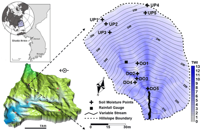
Figure 1Location of the Sulmachun watershed in South Korea with hydrologic monitoring (rainfall and evapotranspiration) stations (lower left) and study area with terrain contours, topographic wetness index (TWI), and soil moisture monitoring points (right).
Rainfall data (used to describe rainfall characteristics) were recorded at hourly intervals using a rainfall gauge (automatic rain gauge system, Eijkelkamp) placed under the canopy. The soil moisture time series were assessed using a multiplex-based time domain reflectometer (TDR; MiniTRASE, SoilMoisture, 2004) at five locations each for upslope (UP1–UP5) and downslope areas (DO1–DO5) (Fig. 1). At each location, three TDR sensors (waveguides) were inserted parallel to the surface at depths of 10, 30, and 60 cm into the upslope side of the installation trench that was filled with soil. Soil moisture measurements were collected hourly between 2007 and 2016. There were 356 rainfall events documented during the study period. A rainfall event was defined as a minimum dry period of 1 d and a minimum of 1 mm of rainfall.
2.2 Data analysis for soil moisture response
For a given rainfall event, the variation in soil moisture at a particular point in the hillslope depends not only on the rainfall, but also on other environmental factors such as the location, depth, and soil texture. To consider the relative variation (%) of water storage normalized by the ASM condition, we used the soil moisture difference index, which is defined as the percentage of maximum soil moisture difference (Zhu et al., 2014), to represent the soil moisture variation as follows:
where θmax represents the maximum soil moisture during a rainfall event and the subsequent period (≤4 h), and θant represents the soil moisture measurement before the rainfall event (2 h).
We also calculated the time from peak to peak (P2P, in h), which is defined as the time difference between the peak of rainfall and the maximum soil moisture variation. The standard deviation of P2P (SDP2P) for the measuring points was used to represent the homogeneity of the soil moisture responses (Kim, 2009). The time series information of the soil moisture was converted to address distinct response features for rainfall events. Depending on the soil moisture responses in the transect, location, and depth, 12 different soil moisture response features were delineated as follows: behavior of all measurements (total); measurements at upslope points (upslope) and those for downslope (downslope); measurements at depths of 10, 30, and 60 cm; measurements for upslope at depths of 10 cm (UP10 cm), 30 cm (UP30 cm), and 60 cm (UP60 cm); and measurements for downslope at depths of 10 cm (DO10 cm), 30 cm (DO30 cm), and 60 cm (DO60 cm).
2.3 Unsupervised machine learning algorithm
The SOM utilizes an unsupervised learning algorithm that can be useful for pattern recognition of multivariate datasets from different observations. The SOM is typically a two-dimensional (2D) grid composed of either hexagonal or rectangular elements. In this study, we used a hexagonal lattice as the output layer because it resulted in better information propagation when updating more neighborhood neurons than those of the rectangular lattice (Kohonen, 2001).
Input variables for the SOM computation were obtained from rainfall features such as rainfall duration (DUR), rainfall amount (AMO), rainfall intensity (INT), ASM, soil moisture difference index and SDP2P for upslope areas at depths of 10, 30, and 60 cm, and those for the downslope areas at depths of 10, 30, and 60 cm, respectively. A log transformation was applied to all input variables to fit the bounds of data between zero and one, except SDP2P, which was <1 in most cases.
SOMs were established for each variable, and the distance between the input vector and weighting vector could be calculated as follows:
where v represents the number of variables.
The best neuron can be identified as the neuron with the minimum value of db, indicating the best fit to the characteristics of each rainfall event among every neuron in the SOM. Once the neuron is selected, the weighting vector should be re-evaluated using Eq. (3) for the renewal weighting vector expressed as follows:
where α (i.e., 0.5) represents the acceleration coefficient, and b represents the winner neuron.
After updating the algorithm, all neurons in the SOMs fit weighting vectors to the multiple datasets used in this study. The input variables in each neuron can be displayed in the component planes, and these are depicted as spatial patterns in SOMs. The nonlinear relationship between variables was identified through visual comparison between the spatially distributed weightings in each component plane (Adeloye et al., 2011; Farsadnia et al., 2014; García and González, 2004; Park et al., 2003).
2.4 Clustering of hydrologic events
Clusters within the dataset can be delineated by applying the dendrogram classification method and by evaluating the dissimilarity between the weighting vectors (Montero and Vilar, 2014). The Euclidean distance function was considered to evaluate the dissimilarity, as it is suitable for deducing shape-based comparisons between soil moisture series whose data are collected simultaneously (Iglesias and Kastner, 2013). This method has also been used to identify clusters of soil moisture data (Van Arkel and Kaleita, 2014). The Euclidean distance between two weighting vectors in neurons (b1 and b2) can be expressed as follows:
The relationship that exhibits the shortest distance between neurons is assigned to the first cluster, and the weighting vectors of the first cluster can be expressed as
where and represent the variable weighting vectors in the neurons (b1 and b2), respectively; and are set to a value of 1 in this relationship, but these values are set to the number of components during the comparison of clusters. Additionally, we used Ward's method to evaluate the dissimilarity between two weighting vectors of each neuron and between each cluster; i.e., this was the chosen algorithm in our hierarchical clustering method (Ward, 1963). When the dissimilarity between two clusters (c1 and c2) is calculated, the distance between clusters can be expressed as
where and represent the averages of clusters c1 and c2, respectively, and and represent the numbers of components for clusters c1 and c2, respectively. A dendrogram can be constructed based on the resulting dcluster, and the upper part from a designated horizontal line can be recognized as the structure of the final clusters.
3.1 Soil moisture responses of all measuring points during rainfall events
The statistics of soil moisture response based on the analysis of 30 points are summarized in terms of the P2P and maximum variation, as displayed in Fig. 2a–f, which present elevations as an order of locations on the x axis as UP1–UP4–UP2–UP5–UP3–DO1–DO2–DO3–DO4–DO5 (Fig. 1) from the hilltop to downslope. The means of P2P ranged from 0.2 to +0.5 d, indicating that the maximum soil moisture could be achieved even before the occurrence of the rainfall peak. Both standard deviation and average of P2P tended to increase at deeper depths, except for locations with elevations of 224 and 216 m (locations of DO2 and DO5 in Fig. 1).
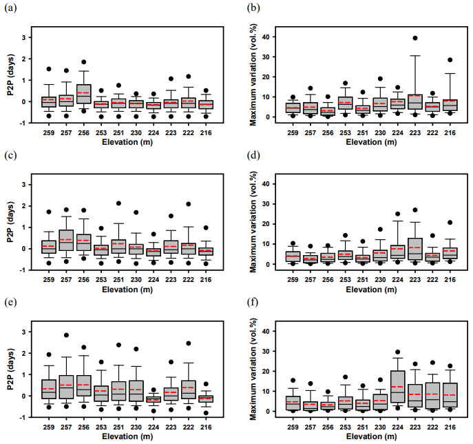
Figure 2Box plots illustrating soil moisture responses of P2P and maximum variation at 10 cm depth (a, b), at 30 cm depth (c, d), and at 60 cm depth (e, f), respectively. Elevations on the x axis are between 260 and 215 m in order of UP1–UP4–UP2–UP5–UP3–DO1–DO2–DO3–DO4–DO5, shown in Fig. 1.
Figure 2a, c, and e indicate that while the mean P2P for the upslope area was 0.24 d, that of the downslope area was 0.02 d. The mean values of P2P at depths of 10, 30, and 60 cm were −0.08, 0.04, and 0.011 d for the downslope and were 0.1, 0.24, and 0.38 d for the upslope, respectively. The differences in P2P between other points at an identical depth for the downslope were smaller than those for the upslope. This suggests that the soil moisture response in the downslope area is faster and more uniform than that in the upslope area. The accumulated soil water flow from the upslope area to the downslope area seems to be responsible for more rapid and less spatially variable soil moisture responses in the downslope area. As shown in Fig. 2b, d, and e, both average and standard deviation of maximum variation tend to increase for locations with lower elevation. The average maximum variations at depths of 10 and 60 cm were higher than those for the 30 cm depth, indicating that primary lateral flow tended to be generated along boundaries (surface and subsurface).
3.2 Soil moisture response features in measuring locations and depths
The soil moisture response features (e.g., ASM, soil moisture difference index, and SDP2P) were expressed in different spatially averaged responses (Fig. 3), depending on the depth and location. As shown in Fig. 3a, the ASM in the downslope area was higher than that in the upslope area. It was apparent that the ASM in the downslope area increased with increasing depth; however, ASM for the upslope area did not display any notable trend in the depth profile. This indicated that soil water infiltration in the upslope area did not necessarily occur for all depth profiles.
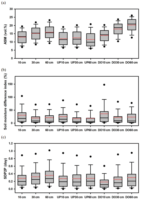
Figure 3Box plots illustrating antecedent soil moisture (a), soil moisture difference index (b), and standard deviation of peak time (SDP2P) (c) of 12 time series of soil moisture.
The soil moisture difference index in the downslope area was higher than that in the upslope area, as shown in Fig. 3b. The average soil moisture difference index in the downslope area (50.67 %) was higher than that of the upslope area (38.73 %), and the average soil moisture difference indices at depths of 10, 30, and 60 cm for the upslope area were 44.51 %, 34.27 %, and 37.39 %, while those for the downslope area were 64.49 %, 40.83 %, and 46.69 %, respectively. This indicates higher wetness along both the surface and subsurface boundaries, and this trend is pronounced in the downslope direction.
The SDP2Ps for the soil moisture datasets represent the degree of spatial heterogeneity in the temporal soil moisture response. The statistics of the SDP2P revealed that the downslope response varied less than the upslope response (Fig. 3c). While the SDP2Ps of the downslope displayed an apparent increasing trend at deeper depths, those for the upslope showed a similar in-depth profile. The difference in the SDP2P profile between the upslope and downslope indicates that the impact of rainfall on soil moisture response timing can be completely different between the upslope and downslope directions.
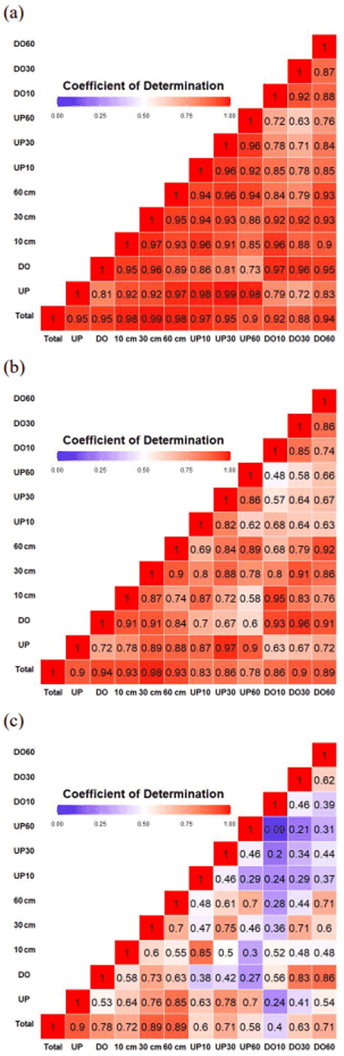
Figure 4Heat maps depicted for the coefficient of determination (R2) among combinations of (a) antecedent soil moisture, (b) soil moisture difference index, and (c) standard deviation of peak time.
The relationships of each response feature (e.g., ASM, soil moisture difference index, and SDP2P) among different soil moisture datasets can be visualized through the heat map presented in Fig. 4. As displayed in Fig. 4, the heat maps for ASM ranged from 0.88–0.99, and those for soil moisture difference indices and SDP2P ranged from 0.78–0.98 and from 0.40–0.90, respectively. The relationships between upslope and downslope (2C2, i.e., the first combination), those between identical depths (3C2, i.e., the second combination), and those for different depths and locations (6C2, i.e., the third combination) indicate the heterogeneity of different soil moisture features in the spatial context. The values for the first combination for ASM, soil moisture difference index, and SDP2P were 0.81, 0.72, and 0.53; the mean values of the second and third combinations were 0.95, 0.84, and 0.62 and 0.83, 0.69, and 0.35 for ASM, soil moisture difference indices, and SDP2P, respectively. This suggested that the spatial distribution of ASM did not demonstrate meaningful spatial variability, but the spatial distributions for soil moisture difference indices and SDP2P were substantial. Therefore, the soil moisture difference index and SDP2P can be deemed useful variables for the characterization of the spatial variation of the soil moisture response for the application of SOM.
3.3 Composition and clustering of SOM
The dataset of hydrologic measurements (356×15) was transformed through the application of 96 neurons and output based on a matrix (16×6) through the iterative application of Eqs. (5) and (6) respectively; i.e., 15 hydrologic variables derived from 356 events were expressed in a compact manner in the SOM. Many alternatives exist in the number of clusters, depending on the complexity of the dendrogram structure. In this study, five clusters were selected based on a heuristic approach to achieve a hydrologically meaningful classification of events and parsimonious clustering. The relation to notable hydrological processes such as lateral flow or vertical preferential flow and the redundancy check in cluster number were essential factors in the implementation of the heuristic approach. Figure 5a illustrates the resulting dendrogram for the five clusters. The structure of the dendrogram demonstrates the relationships between groups of clusters and between individual clusters. Figure 5b presents the output SOM (16×6) delineated from the dendrogram analysis, which is a structural array identical to the delineated dendrogram with neurons for each cluster. The spatial distributions between other clusters and the corresponding numbers of neurons indicate the areal portion of each cluster from all clusters and their connections with adjacent clusters.
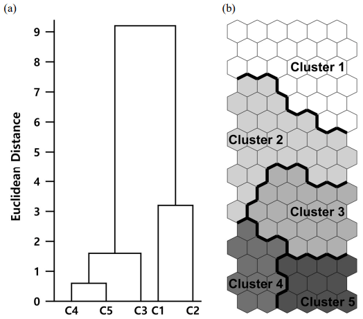
Figure 5Structure of (a) dendrogram for five clusters and (b) SOM classifications in 96 neurons through the application of a 16×6 matrix.
Table 1 presents the average of vector components, such as the AMO, DUR, INT, and average ASM among all measuring points (ASMTOT) in volume percent, along with an average of the soil moisture difference indices (Δθ) in five upslope locations and five downslope locations at depths of 10, 30, and 60 cm, as VUP10, VUP30, VUP60, VDO10, VDO30, and VDO60. Additionally, it presents the SDP2P in five upslope and five downslope locations at depths of 10, 30, and 60 cm, as SUP10, SUP30, SUP60, SDO10, SDO30, and SDO60, respectively, for the five clusters displayed in Fig. 5b.
Table 1Arithmetic averages of SOM inputs for rainfall amount (AMO), rainfall duration (DUR), rainfall intensity (INT), antecedent soil moisture for all points (ASMTOT), volumetric soil moisture difference index, and standard deviation of peak-to-peak time (SDP2P).
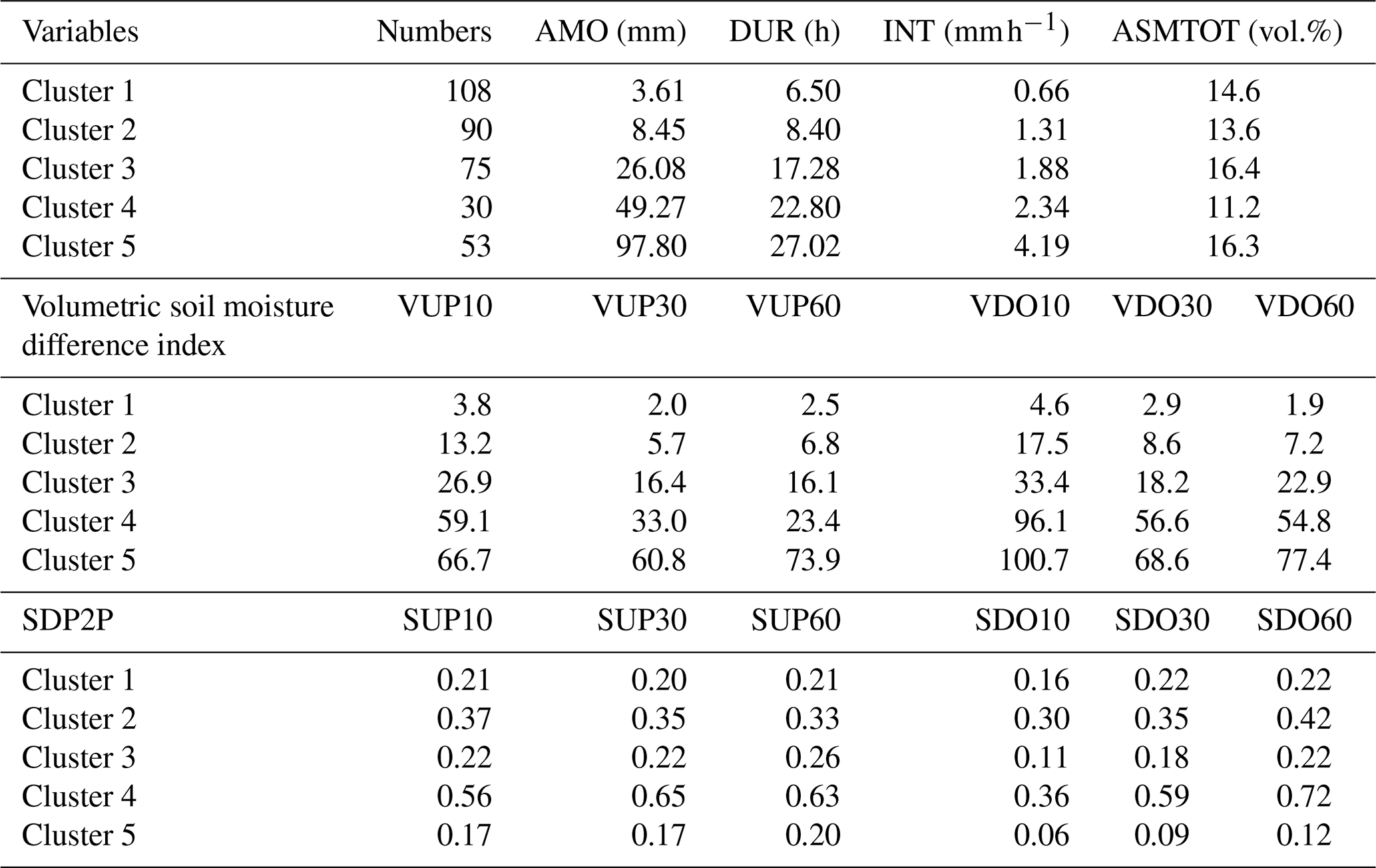
As displayed in Fig. 5b, Clusters 1 and 2 were located in the upper part of the SOM. Table 1 indicates that the rainfall characteristics of Clusters 1 and 2, such as DUR, AMO, and INT, were relatively low, but those for the ASM were similar to the mean ASM for all clusters (Table 1). The average soil moisture difference indices were less than 5 % for Cluster 1 because the low AMO and intensity resulted in a limited increase in soil water storage, and the loss due to evaporation offset a substantial proportion of the precipitation (Albertson and Kiely, 2001; Ramirez et al., 2007). Cluster 2 exhibited higher AMO and intensities and more significant average soil moisture differences indices than Cluster 1 (Table. 1). The intermediate part of the SOM (Fig. 5b) was associated with Cluster 3, which revealed higher rainfall durations, quantities, and intensities than those for Clusters 1 and 2, which resulted in a higher soil moisture difference index for Cluster 3 than for Clusters 1 and 2 (Table 1). One notable feature of Cluster 3 was the increasing trend of soil moisture difference indices with depth (DO60 > DO30) for the downslope area, whereas Clusters 1 and 2 displayed decreased soil moisture difference indices with depth (DO30 > DO60) (Table 1). The pattern of soil moisture difference index for Cluster 3 suggests vertical infiltration in all depth profiles for upslope and apparent lateral flow for downslope areas (Table 1 and Fig. 4), which seems to be completely different from Clusters 1 and 2. Clusters 4 and 5 demonstrated a greater soil moisture difference index, with significant events in the SOM classification (Table 1). Cluster 4 displayed two distinctive features compared to other clusters. Firstly, the ASM of Cluster 4 was the lowest among all clusters. However, the soil moisture difference indices at depths of 30 and 60 cm in the downslope area for Cluster 4 were significantly higher than those in Clusters 1, 2, and 3. Secondly, the difference in soil moisture difference index between the upslope and downslope areas was the most pronounced in Cluster 4. This suggests that the hydrological processes in the upslope and downslope areas can be substantially distinct from each other. Both rainfall characteristics and soil moisture difference index for Cluster 5 were significantly higher than those for all other clusters. Several measurement data points in Cluster 5 exhibited saturation during rainfall events, and the soil moisture at a depth of 60 cm displayed higher variation than that at 30 cm, which indicated that subsurface stormflow was generated along the bedrock in both the upslope and downslope areas.
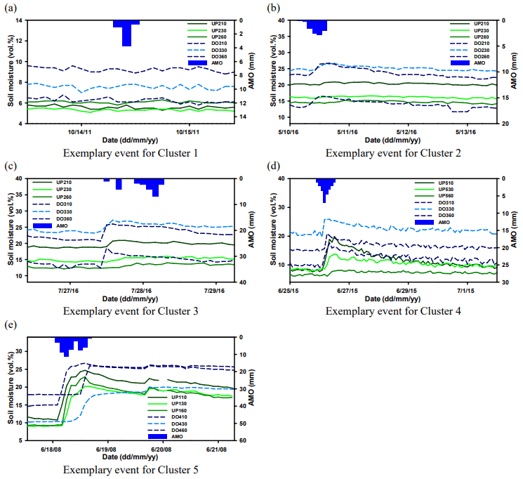
The centroid for each cluster was calculated by averaging combinations of weighting vectors in the neurons. The event having the smallest root mean squared error between input variables of each event and the centroid of each cluster was selected as the exemplary event for corresponding cluster. Appendix A presents exemplary events with rainfall and soil moisture responses at several upslope and downslope points for Clusters 1 to 5. The exemplary event for Cluster 1 showed almost no response to rainfall, and that of Cluster 2 resulted in limited responses in designated downslope locations. Both events from Clusters 3 and 4 showed an apparent response in many points, with a difference in lower antecedent soil moisture condition for Cluster 4. The exemplary event for Cluster 5 showed significant recharge impact in soil moisture for most points.
3.4 Component planes for variables
Information on the component planes of 16 variables and their visual comparisons can help provide insights into the nonlinear relationships between the 16 hydrological variables. Figure 6 illustrates the SOM distributions for the component weightings of the 16 variables. Both the spatial distributions and the scales of weightings (scale bar) in Fig. 6 represent the characteristics of impacts (rainfall features and ASM) and consequences (average of soil moisture difference and SDP2P).
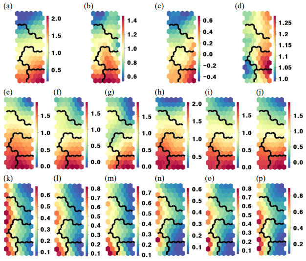
Figure 6(a–p) Component planes of variable weightings for rainfall amount (AMO) (a); rainfall duration (DUR) (b); rainfall intensity (INT) (c); antecedent soil moisture (ASM) (d); soil moisture difference indices for the upslope and downslope at depths of 10, 30, and 60 cm (VUP10, VUP30, VUP60, VDO10, VDO30, and VDO60) (e–j); standard deviation of peak time for the upslope and downslope at depths of 10, 30, and 60 cm (SUP10, SUP30, SUP60, SDO10, SDO30, and SDO60) (k–p).
The visual comparison of Fig. 6a–d indicates a negligible relationship between rainfall features and ASM. The component planes for upslope soil moisture difference indices at depths of 10, 30, and 60 cm (Fig. 6e–g) displayed similar spatial weightings to those for rainfall features. The high weightings for the soil moisture difference index at a 10 cm depth were mainly distributed to Clusters 4 and 5, and the weightings tended to concentrate in Cluster 5 at higher values of depths (Fig. 5). The comparison between ASM and soil moisture difference index indicated that ASM did not influence the soil moisture difference index.
The exclusive vertical flow impact can be proposed as one possible explanation for the relationship between the component plane for VUP10 and the component planes for VUP30 or VUP60 (Fig. 6e, f, and g) because there were negligible contributing areas or small values of topographic wetness indices (Fig. 1) in upslope locations. Weightings in VUP10 were associated with AMO and INT, but those for VUP60 correlated only with AMO. This pattern of weighting shift was observed between VUP30 and VUP60, which could be attributed to the effect of vertical infiltration (Li et al., 2013). This relationship along the vertical profile differed between the upslope and downslope. The development of the vertical gradient in weightings (Fig. 6e–g) from VUP10 to VUP60 can barely be observed in weightings from VDO10 to VDO60 (Fig. 6h–j). This suggests that the flow path in the downslope area cannot be completely explained by the vertical flow.
Figure 6k–m display the component planes of SDP2P at depths of 10, 30, and 60 cm in the upslope area. The weighting distributions between upslope SDP2P (Fig. 6k–m) and ASM (Fig. 6d) were completely reversed. The spatial distribution of SDP2P in the downslope did not reveal a notable difference in the in-depth profile (Fig. 6n–p). This could be explained by the possibility that the time to peak in the downslope was not only determined by rainfall, but it was more affected by other drivers such as topography.
4.1 Characterization of the classified hydrologic events
The hydrologic events classified by the SOM can be characterized through a comparative feature presentation for all clusters (Fig. 7). The lower ASM matched with a higher mean and wider bound in SDP2P, which could also be confirmed by the component planes of ASM and SDP2P. With increasing depth, the heterogeneity in response time increased (greater SDP2P) in most locations. This can be explained by the response time between rainfall and soil moisture decreasing with depth. The SDP2P response between the upslope and downslope can be distinctly expressed depending on the cluster. Clusters 1 and 2 exhibited negligible differences in hillslope transects, but those for Clusters 3, 4, and 5 were substantially different. This is because the generation of lateral flow can be more significant under greater rainfall events in downslope areas than in upslope areas. The soil moisture peak formations matched well with the soil moisture difference indices in soil moisture at the downslope. Events in Cluster 1 demonstrated less variation in SDP2P for both depth profile and hillslope transact location because of the lowest AMO and INT values. The impact of depth on the variation of SDP2P can be observed in Clusters 2, 3, and 5, and with increasing depth, the bound was higher in both upslope and downslope areas. However, this pattern was different between the upslope and downslope in Cluster 4 that presented the lowest ASM. The lowest ASM led to substantially less response variation at a 60 cm depth in the upslope, while that for the downslope revealed higher variation at a 60 cm depth compared to that reported at shallower depths. This suggested that the dominant flow path between the upslope and downslope was different in Cluster 4.
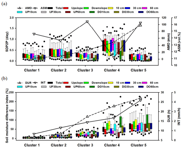
Figure 7SDP2Ps with mean AMO and ASM for each cluster (a) soil moisture difference indices with mean DUR and INT for each cluster (b) for total, upslope, and downslope at depths of 10, 30, and 60 cm, and the corresponding depths for upslope and downslope.
The increasing pattern of the soil moisture difference indices corresponds to increasing rainfall features such as DUR and INT from Clusters 1 to 5. However, the depth profile of the soil moisture difference index differed between Clusters 4 and 5. While the scale of soil moisture recharge demonstrated an apparent decrease in the depth profile for Cluster 4, that for Cluster 5 demonstrated different surface and subsurface boundaries (at depths of 10 and 60 cm). This indicated that the dominant hydrological processes for Cluster 4 appear restricted to the surface as the vertical flow, but those for Cluster 5 existed at both the surface and subsurface boundaries as both vertical and lateral flows.
The impact of rainfall events on water storage can be useful for understanding the changes in various hydrological statuses for each cluster. The storage changes (Table 2) were estimated by multiplying the soil moisture change by the corresponding depth for each waveguide (e.g., 200 mm for 10 and 30 cm depths, and 300 mm for 60 cm depth). Water storage analysis for Cluster 1 demonstrated negligible changes under 2 % (the measurement accuracy of TDR) in soil moisture that occurred in both the upslope and downslope areas. Rainfall impacts to Cluster 2 can be classified as an intermediate category because both clusters introduced remarkable storage changes (mm) in the downslope area. Significant changes in water storage were observed for Clusters 3, 4, and 5, regardless of the quantity of rainfall. Substantial increases in storage change at a depth of 60 cm in the downslope area indicated the generation of subsurface stormflow for Clusters 3, 4, and 5. The main difference between Clusters 3, 4, and 5 was in terms of whether the subsurface lateral flow was generated in the upslope area. Clusters 3 and 5 could be characterized by high rainfall and high ASM, which resulted in subsurface lateral flow in both the upslope and downslope areas. The soil moisture changes and storage for Cluster 4 indicated an apparent decreasing trend in the depth profile in the upslope area. The storage changes and soil moisture difference indices at depths of 10 and 30 cm in the upslope area for Cluster 4 were greater than those for Cluster 3 due to higher AMO, DUR, and INT. However, the storage change at a depth of 60 cm in the upslope for Cluster 4 was smaller than that of Cluster 3, which could be explained by the lower infiltration under comparatively dry ASM conditions (Zhu et al., 2014; Mei et al., 2018; He et al., 2020). The machine learning algorithm (SOM) can be considered a useful analysis platform, not only for elucidating soil moisture response patterns in conjunction with rainfall and ASM (Fig. 7), but also for an effective characterization of soil water storage changes at different locations and depths (Table 2).
Table 2Soil moisture changes and storage changes for all clusters at depths of 10, 30, and 60 cm and those recorded for upslope and downslope.
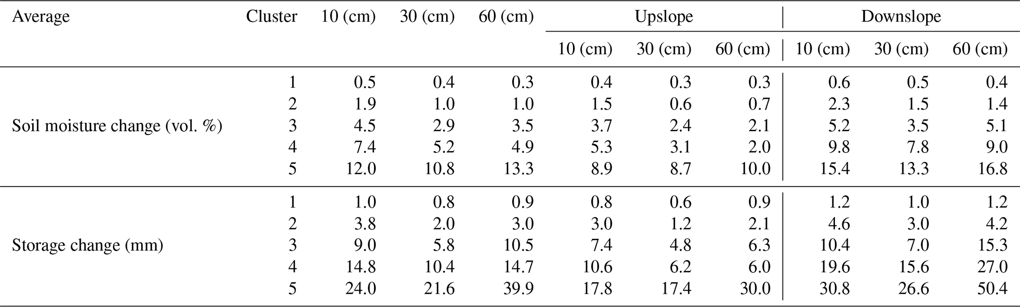
Table 3Combinations of flow paths and its hydrologic conditions for all clusters.
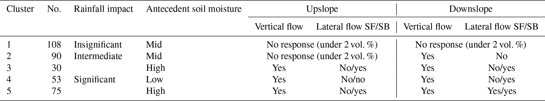
SF: surface; SB: subsurface.
4.2 Configuration of hydrological processes
The application of SOM, an unsupervised machine learning algorithm, to the dataset provided an integrated assessment for the evaluation and characterization of hydrologic events. The recharge patterns of water storage for the soil layers of the hillslope were characterized by several distinct clusters. The distinct distribution of characteristics of soil moisture responses could be explained by the different combinations of drivers (rainfall and ASM) and hydrological processes (vertical flow, surface, and subsurface lateral flows) for each cluster. The hillslope hydrological flow path was characterized by comparing the component planes between UP10 and UP30 or UP60 and other combinations of soil moisture component planes, such as those of DO10 and DO30 or DO60 regarding SDP2P and soil moisture difference index.
The rainfall events can be classified into three distinct categories, which depend on the rainfall characteristics, and five refined clusters as follows: insignificant events for Cluster 1, intermediate events for Cluster 2, and significant events for Clusters 3, 4, and 5 (Table 3). Further classification of significant events indicated that the effects of antecedent moisture conditions and AMO were critical for delineating Clusters 3, 4, and 5. The generation of hydrological processes based on significant soil moisture changes over 2 % and increasing patterns of SDP2P (0.11 for 10 cm, 0.18 for 30 cm, and 0.22 for 60 cm, respectively) at greater depths was the threshold feature between the insignificant and intermediate events. The primary difference between the intermediate and significant events was deemed the significant response in both the upslope and downslope areas and the substantial development of interface flow between the bedrock and soil layer in the downslope area. This indicated that the lateral flow along boundaries (subsurface and surface) was stronger than that at intermediate depths, and the downslope lateral flow tended to be generated through boundaries either along the surfaces or bedrock. Furthermore, ASM was substantially higher for Clusters 3 and 5 than that for Cluster 4, and the SDP2Ds in Clusters 3 and 5 were lower for all points than those for Cluster 4. This can be explained by the development of preferential pipe flow, which is more common at greater depths under comparatively wet conditions (Lai et al., 2016; Uber et al., 2018; Uchida et al., 2001; Wienhöfer and Zehe, 2014). Low variation and soil moisture changes in UP60 for Cluster 4 indicated that low antecedent moisture conditions could limit the generation of lateral flow in the upslope area, and for Cluster 3, this could be explained by even fewer rainfall events than in Cluster 4, and these were sufficient to activate subsurface lateral flow in the upslope. Extreme rainfall events were mainly associated with Cluster 5. Lateral storm flow likely occurred in both the upslope and downslope areas of Cluster 5. Effective drainage during extreme events seems to be strongly associated with lateral flow generation along the two boundaries in the soil media (i.e., surface and bedrock) (Angermann et al., 2017; Freer et al., 2004; Haga et al., 2005; Kim, 2009; Uchida et al., 2001; Wienhöfer and Zehe, 2014). The impact of extreme rainfall conditions dominates other controls (e.g., land cover and topography) regarding hillslope runoff generation (Feng and Liu, 2015).
As presented in Table 3, delineated clusters of hydrologic events can be considered to distinctly explain the combinations of hydrological processes such as vertical and lateral flows (either surface and subsurface boundaries) between the upslope and downslope directions. Events from Cluster 1 were insignificant in terms of the hydrologic response, and the primary driver of Cluster 2 was rainfall that partially affected soil water storage (downslope). While the bedrock topography was important for Clusters 3, 4, and 5, the surface topography played an important role for Cluster 5.
Several studies have been conducted to model the behavior of hillslope hydrology (Fan et al., 2019; Loritz et al., 2017). The SOM analysis for a large dataset showed an apparent distinct pattern in soil moisture response and flow path generation between upslope and downslope areas depending on antecedent soil moisture and rainfall conditions. This suggests that the performance of the model can be improved as the storage structure of the model (fast and slow reservoirs) (Gao et al., 2014; Gharari et al., 2014) is further classified into upslope and downslope categories. The appearance of Cluster 4 (Table 3) demonstrates nonlinear behaviors in the hydrologic response, which can be explained by the apparent role of macropore flow. even under low soil moisture conditions (Beven and Germann, 2013; Nimmo, 2012). The implementation of bypass flow under low ASM and high rainfall conditions into the model structure can help improve the modeling of soil water travel time (Kim, 2014). Further elaboration in modeling to represent dual lateral boundary flows in Cluster 5 can be useful to address multiple drain flow pathways under extreme rainfall conditions.
Rainfall characteristics and responses of soil moisture at the hillslope scale were explored by applying SOM to a dataset comprising information on a considerable number of hydrologic events. Hydrologic events were characterized using rainfall and soil moisture data collected over a period of 10 years from a steep hillside. Based on a delineated dendrogram, the classification of neurons into five clusters provided meaningful interpretations for understanding hydrologic events.
The nonlinear relationships between the hydrologic variables were effectively expressed in the 2D SOM presentations of the variables. The apparent relationship between ASM and peak time variation indicates that the hydrologic response is more feasible under comparatively wet conditions. Water storage analysis for each event from different clusters suggests that spatially different combinations of soil moisture difference index can be attributed to the identified hydrologic response for each cluster. Combinations of upslope and downslope spatial patterns of hillslope hydrological processes, vertical flow, and lateral flow along surface or subsurface boundaries were attributable to the distinctions observed between the event clusters. Depending on the rainfall and ASM conditions delineated from each cluster, the spatial distribution of hydrological processes can be predicted to be useful for obtaining systematic insights into the hillslope hydrological response. The SOM can be considered a useful analysis tool, not only to understand the different soil moisture response patterns between the upslope and downslope areas, but also to configure particular hydrological processes for delineated clusters. The meta-heuristic classification of hydrologic events provides a better understanding of hydrologic conditions and their drivers, which is vital for designing a process-based hillslope hydrology model.
The code is available on request from the authors. The data have been uploaded as the Supplement.
The supplement related to this article is available online at: https://doi.org/10.5194/hess-25-5733-2021-supplement.
EL, SK, and several former graduate students collected data for the study area. EL developed the model code and performed simulations. SK drafted and revised the manuscript. Both authors have approved the final version of the manuscript.
The contact author has declared that neither they nor their co-authors have any competing interests.
Publisher’s note: Copernicus Publications remains neutral with regard to jurisdictional claims in published maps and institutional affiliations.
The authors appreciate the constructive comments from the reviewers and the editor.
This research has been supported by the National Research Foundation of Korea (grant no. 2016R1D1A1B02008137).
This paper was edited by Erwin Zehe and reviewed by Uwe Ehret and one anonymous referee.
Adeloye, A. J., Rustum, R., and Kariyama, I. D.: Kohonen self-organizing map estimator for the reference crop evapotranspiration, Water Resour. Res., 47, W08523, https://doi.org/10.1029/2011WR010690, 2011.
Ahmad, S., Kalra, A., and Stephen, H.: Estimation soil moisture using remote sensing data: A machine learning approach, Adv. Water Resour., 33, 69–80, https://doi.org/10.1016/j.advwatres.2009.10.008, 2010.
Albertson, J. D. and Kiely, G.: On the structure of soil moisture time series in the context of land surface models, J. Hydrol, 243, 101–119, https://doi.org/10.1016/S0022-1694(00)00405-4, 2001.
Ali, M., Fiori, A., and Bellotti, G.: Analysis of the nonlinear storage-discharge relation for hillslopes through 2D numerical modelling, Hydrol. Process., 27, 2683–2690, https://doi.org/10.1002/hyp.9397, 2013.
Angermann, L., Jackisch, C., Allroggen, N., Sprenger, M., Zehe, E., Tronicke, J., Weiler, M., and Blume, T.: Form and function in hillslope hydrology: characterization of subsurface flow based on response observations, Hydrol. Earth Syst. Sci., 21, 3727–3748, https://doi.org/10.5194/hess-21-3727-2017, 2017.
Bachmair, S., Weiler, M., and Troch, P. A.: Intercomparing hillslope hydrological dynamics: Spatio-temporal variability and vegetation cover effects, Water Resour. Res., 48, W05537, https://doi.org/10.1029/2011WR011196, 2012.
Baroni, G., Ortuani, B., Facchi, A., and Gandolfi, C.: The role of vegetation and soil properties on the spatio-temporal variability of the surface soil moisture in a maize-cropped field, J. Hydrol., 489, 148–159, https://doi.org/10.1016/j.jhydrol.2013.03.007, 2013.
Beven, K. and Germann, P.: Macropores and water flow in soils revisited, Water Resour. Res., 49, 3071–3092, https://doi.org/10.1002/wrcr.20156, 2013.
Carranza, C., Nolet, C., Pejij, M., and van der Ploeg, M.: Root zone soil moisture estimation with random forest, J. Hydrol., 593, 125840, https://doi.org/10.1016/j.jhydrol.2020.125840, 2021.
Casper, M. C., Grigoryan, G., Gronz, O., Gutjahr, O., Heinemann, G., Ley, R., and Rock, A.: Analysis of projected hydrological behavior of catchments based on signature indices, Hydrol. Earth Syst. Sci., 16, 409–421, https://doi.org/10.5194/hess-16-409-2012, 2012.
Castillo, V. M., Gomez-Plaza, A., and Martinez-Mena, M.: The role of antecedent soil water content in the runoff response of semiarid catchments: a simulation approach, J. Hydrol., 284, 114–130, https://doi.org/10.1016/S0022-1694(03)00264-6, 2003.
Chen, I. T., Chang, L. C., and Chang, F. J.: Exploring the sptio-temporal interrelation between groundwater and surface water by using the self-organizing maps, J. Hydrol., 556, 131–142, https://doi.org/10.1016/j.jhydrol.2017.10.015, 2018.
Crow, W. T. and Ryu, D.: A new data assimilation approach for improving runoff prediction using remotely-sensed soil moisture retrievals, Hydrol. Earth Syst. Sci., 13, 1–16, https://doi.org/10.5194/hess-13-1-2009, 2009.
Curtu, R., Mantilla, R., Fonley, M., Cunha, L. K., Small, S. J., Jay, L. O., and Krajewski, W. F.: An integral-balance nonlinear model to simulate changes in soil moisture, groundwater and surface runoff dynamics at the hillslope scale, Adv. Water Resour., 71, 125–139, https://doi.org/10.1016/j.advwatres.2014.06.003, 2014.
Di Prinzio, M., Castellarin, A., and Toth, E.: Data-driven catchment classification: application to the pub problem, Hydrol. Earth Syst. Sci., 15, 1921–1935, https://doi.org/10.5194/hess-15-1921-2011, 2011
Farsadnia, F., Kamrood, M. R., Nia, A. M., Modarres, R., Bray, M. T., Han, D., and Sadatinejad, J.: Identification of homogeneous regions for regionalization of watersheds by two-level self-organizing feature maps, J. Hydrol., 509, 387–397, https://doi.org/10.1016/j.jhydrol.2013.11.050, 2014.
Fan, Y., Clark, M., Lawrence, D. M., Swenson, S., Band, L. E., Brantley, S. L., Brooks, P. D., Dietrich, W. E., Flores, A., Grant, G., Kirchner, J. W., Mackay, D. S., McDonnell, J. J., Milly, P. C. D., Sullivan, P. L., Tague, C., Ajami, H., Chaney, N., Hartmann, A., Hazenberg, P., McNamara, J., Pelletier, J., Perket, J., Rouholahnejad-Freund, E., Wagener, T., Zeng, X., Beighley, E., Buzan, J., Huang, M., Livneh, B., Mohanty, B. P., Nijssen, B., Safeeq, M., Shen, C., Verseveld, W. van, Volk, J., and Yamazaki, D.: Hillslope hydrology in global change research and earth system modeling, Water Resour. Res., 55, 1737–1772, https://doi.org/10.1029/2018WR023903, 2019.
Feng, H. and Liu, Y.: Combined effects of precipitation and air temperature on soil moisture in different land covers in a humid basin, J. Hydrol., 531, 1129–1140, https://doi.org/10.1016/j.jhydrol.2015.11.016, 2015.
Freer, J., McDonnell, J., Beven, K., Peters, N. E., Burns, D. A., Hooper, R. P., Aulenbach, B., and Kendall, C.: The role of bedrock topography on subsurface storm flow, Water Resour. Res., 38, W1269, https://doi.org/10.1029/2001WR000872, 2004.
Gao, H., Hrachowitz, M., Fenicia, F., Gharari, S., and Savenije, H. H. G.: Testing the realism of a topography-driven model (FLEX-Topo) in the nested catchments of the Upper Heihe, China, Hydrol. Earth Syst. Sci., 18, 1895–1915, https://doi.org/10.5194/hess-18-1895-2014, 2014.
Gharari, S., Hrachowitz, M., Fenicia, F., Gao, H., and Savenije, H. H. G.: Using expert knowledge to increase realism in environmental system models can dramatically reduce the need for calibration, Hydrol. Earth Syst. Sci., 18, 4839–4859, https://doi.org/10.5194/hess-18-4839-2014, 2014.
Gwak, Y. and Kim, S.: Factors affecting soil moisture spatial variability for a humid forest hillslope, Hydrol. Process., 31, 431–445, https://doi.org/10.1002/hyp.11039, 2016.
Haga, H., Matsumoto, Y., Matsutani, J., Fujita, M., Nishida, K., and Sakamoto, Y.: Flow paths, rainfall properties, and antecedent soil moisture controlling lags to peak discharge in a granitic unchanneled catchment, Water Resour. Res., 41, W12410, https://doi.org/10.1029/2005WR004236, 2005.
Hardie, M. A., Cotching, W. E., Doyle, R. B., Holz, G., Lisson, S., and Mattern, K.: Effect of antecedent soil moisture on preferential flow in a texture-contrast soil, J. Hydrol., 398, 191–201, https://doi.org/10.1016/j.jhydrol.2010.12.008, 2011.
He, Z., Zhao, W., Liu, H., and Chang, X.: The response of soil moisture to rainfall event size in subalpine grassland and meadows in a semi-arid mountain range: a case study in northwestern China's Qilian Mountains, J. Hydrol., 420–421, 183–190, https://doi.org/10.1016/j.jhydrol.2011.11.056, 2012.
He, Z., Jia, G., Liu, Z., Zhang, Z., Yu, X., and Xiao, P.: Field studies on the influence of rainfall intensity, vegetation cover and slope length on soil moisture infiltration on typical watersheds of the Loess Plateau, China, Hydrol. Process., 34, 4904–4919, https://doi.org/10.1002/hyp.13892, 2020.
Heisler-White, J. L., Knapp, A. K., and Kelly, E. F.: Increasing precipitation event size increases aboveground net primary productivity in a semi-arid grassland, Oecologia, 158, 129–140, https://doi.org/10.1007/s00442-008-1116-9, 2008.
Herbst, M., Gupta, H. V., and Casper, M. C.: Mapping model behaviour using Self-Organizing Maps, Hydrol. Earth Syst. Sci., 13, 395–409, https://doi.org/10.5194/hess-13-395-2009, 2009.
Iglesias, F. and Kastner, W.: Analysis of similarity measures in times series clustering for the discovery of building energy patterns, Energies, 6, 579–597, https://doi.org/10.3390/en6020579, 2013.
Ismail, S., Shabri, A., and Samsudin, R.: A hybrid model of self organizing maps and least square support vector machine for river flow forecasting, Hydrol. Earth Syst. Sci., 16, 4417–4433, https://doi.org/10.5194/hess-16-4417-2012, 2012.
Kim, S.: Characterization of soil moisture responses on a hillslope to sequential rainfall events during late autumn and spring, Water Resour. Res., 45, W09425, https://doi.org/10.1029/2008WR007239, 2009.
Kim, S.: Hydrometric Transit Times along Transects on a Steep Hillslope, Water Resour. Res., 50, 7267–7284, https://doi.org/10.1002/2013WR014746, 2014.
Kohonen, T.: Self-Organizing Maps, third edn., Springer, Berlin, ISBN 978-3-642-56927-2, 2001.
Lai, X., Liao, K., Feng, H., and Zhu, Q.: Responses of soil water percolation to dynamic interactions among rainfall, antecedent moisture and season in forest site, J. Hydrol., 540, 565–573, https://doi.org/10.1016/j.jhydrol.2016.06.038, 2016.
Lee, E. and Kim, S.: Characterization of runoff generation in a mountainous hillslope according to multiple threshold behavior and hysteretic loop features, J. Hydrol., 590, 125534, https://doi.org/10.1016/j.jhydrol.2020.125534, 2020.
Ley, R., Casper, M. C., Hellebrand, H., and Merz, R.: Catchment classification by runoff behaviour with self-organizing maps (SOM), Hydrol. Earth Syst. Sci., 15, 2947–2962, https://doi.org/10.5194/hess-15-2947-2011, 2011.
Li, X. Y., Zhang, S. Y., Peng, H. Y., Hu, X., and Ma, Y. J.: Soil water and temperature dynamics in shrub-encroached grasslands and climatic implications: Results from inner Mongolia steppe ecosystem of north China, Agr. Forest Meteorol., 171, 20–30, https://doi.org/10.1016/j.agriformet.2012.11.001, 2013.
Liang, W. L., Kosugi, K., and Mizuyama, T.: Soil water dynamics around a tree on a hillslope with or without rainwater supplied by stemflow, Water Resour. Res., 47, W02541, https://doi.org/10.1029/2010WR009856, 2011.
Liao, K., Zhou, Z., Lai, X., Zhu, Q., and Feng, H.: Evaluation of different approaches for identifying optimal sites to predict mean hillslope soil moisture content, J. Hydrol., 547, 10–20, 10.1016/j.jhydrol.2017.01.043, 2017.
López García, H. and Machón González, I.: Self-organizing map and clustering for wastewater treatment monitoring, Eng. Appl. Artif. Intel., 17, 215–225, https://doi.org/10.1016/j.engappai.2004.03.004, 2004.
Loritz, R., Hassler, S. K., Jackisch, C., Allroggen, N., van Schaik, L., Wienhöfer, J., and Zehe, E.: Picturing and modeling catchments by representative hillslopes, Hydrol. Earth Syst. Sci., 21, 1225–1249, https://doi.org/10.5194/hess-21-1225-2017, 2017.
Lu, N. and Godt, J.: Infinite slope stability under steady unsaturated seepage conditions, Water Resour. Res., 44, W11404, https://doi.org/10.1029/2008WR006976, 2008.
Mei, X., Zhu, Q., Ma, L., Zhang, D., Wang, Y., and Hao, W.: Effect of stand origin and slope position on infiltration pattern and preferential flow on a Loess hillslope, Land Degrad. Dev., 29, 1353–1365, https://doi.org/10.1002/ldr.2928, 2018.
Montero, P. and Vilar, J. A.: TSclust: An R package for time series clustering, J. Stat. Softw., 62, 1–43, https://doi.org/10.18637/jss.v062.i01, 2014.
Nimmo, J. R.: Preferential flow occurs in unsaturated conditions, Hydrol. Process., 26, 786–789, https://doi.org/10.1002/hyp.8380, 2012.
Park, Y. S., Cereghino, R., Compin, A., and Lek, S.: Applications of artificial neural networks for pattering and predicting aquatic insect species richness in running waters, Ecol. Model., 160, 265–280, https://doi.org/10.1016/S0304-3800(02)00258-2, 2003.
Penna, D., Borga, M., Norbiato, D., and Fontana, G. D.: Hillslope scale soil moisture variability in a steep alpine terrain, J. Hydrol., 364, 311–327, https://doi.org/10.1016/j.jhydrol.2008.11.009, 2009.
Penna, D., Tromp-van Meerveld, H. J., Gobbi, A., Borga, M., and Dalla Fontana, G.: The influence of soil moisture on threshold runoff generation processes in an alpine headwater catchment, Hydrol. Earth Syst. Sci., 15, 689–702, https://doi.org/10.5194/hess-15-689-2011, 2011.
Ramirez, D. A., Bellot, J., Domingo, F., and Blasco, A.: Can water responses in stipa tenacissima L. during the summer season be promoted by non-rainfall water gains in soil?, Plant Soil, 291, 67–79, https://doi.org/10.1007/s11104-006-9175-3, 2007.
Reusser, D. E., Blume, T., Schaefli, B., and Zehe, E.: Analysing the temporal dynamics of model performance for hydrological models, Hydrol. Earth Syst. Sci., 13, 999–1018, https://doi.org/10.5194/hess-13-999-2009, 2009.
Rodriguez-Iturbe, I., Isham, V., Cox, D. R., Manfreda, S., and Porporato, A.: Space-time modeling of soil moisture: Stochastic rainfall forcing with heterogeneous vegetations, Water Resour. Res., 42, W06D05, https://doi.org/10.1029/2005WR004497, 2006.
Rosenbaum, U., Bogena, H. R., Herbst, M., Huisman, J. A., Peterson, T. J., Weuthen, A., Western, A. W., and Vereecken, H.: Seasonal and event dynamics of spatial soil moisture patterns at the small catchment scale, Water Resour. Res., 48, W10544, https://doi.org/10.1029/2011WR011518, 2012.
Saffarpour, S., Western, A. W., Adams, R., and McDonnell, J. J.: Multiple runoff processes and multiple thresholds control agricultural runoff generation, Hydrol. Earth Syst. Sci., 20, 4525–4545, https://doi.org/10.5194/hess-20-4525-2016, 2016.
Shrestha, D. L., Kayastha, N., and Solomatine, D. P.: A novel approach to parameter uncertainty analysis of hydrological models using neural networks, Hydrol. Earth Syst. Sci., 13, 1235–1248, https://doi.org/10.5194/hess-13-1235-2009, 2009.
Srivastava, P. K., Han, D., Ramirez, M. R., and Islam, T.: Machine learning techniques for downscaling smos satellite soil moisture using modis land surface temperature for hydrological application, Water Resour. Manag., 27, 3127–3144, https://doi.org/10.1007/s11269-013-0337-9, 2013.
Toth, E.: Catchment classification based on characterisation of streamflow and precipitation time series, Hydrol. Earth Syst. Sci., 17, 1149–1159, https://doi.org/10.5194/hess-17-1149-2013, 2013.
Tramblay, Y., Bouaicha, R., Brocca, L., Dorigo, W., Bouvier, C., Camici, S., and Servat, E.: Estimation of antecedent wetness conditions for flood modelling in northern Morocco, Hydrol. Earth Syst. Sci., 16, 4375–4386, https://doi.org/10.5194/hess-16-4375-2012, 2012.
Tromp van Meerveld, I. and McDonnell, J. J.: Comment to “Spatial correlation of soil moisture in small catchments and its relationship to dominant spatial hydrological processes, Journal of Hydrology, 286, 113–134”, J. Hydrol., 303, 307–312, https://doi.org/10.1016/j.jhydrol.2004.09.002, 2005.
Uber, M., Vandervaere, J.-P., Zin, I., Braud, I., Heistermann, M., Legoût, C., Molinié, G., and Nord, G.: How does initial soil moisture influence the hydrological response? A case study from southern France, Hydrol. Earth Syst. Sci., 22, 6127–6146, https://doi.org/10.5194/hess-22-6127-2018, 2018.
Uchida, T., Kosugi, K., and Mizuyama, T.: Effects of pipeflow on hydrological process and its relations to landslide, a review of pipeflow studies in forested headwater catchments, Hydrol. Process., 15, 2151–2174, https://doi.org/10.1002/hyp.281, 2001.
Van Arkel, Z. and Kaleita, A. L.: Identifying sampling locations for field-scale soil moisture estimation using K-means clustering, Water Resour. Res., 50, 7050–7057, https://doi.org/10.1002/2013WR015015, 2014.
Wang, S., Fu, B., Gao, G., Liu, Y., and Zhou, J.: Responses of soil moisture in different land cover types to rainfall events in a re-vegetation catchment area of the Loess Plateau, China, Catena, 101, 122–128, https://doi.org/10.1016/j.catena.2012.10.006, 2013.
Wang, X. P., Cui, Y., Pan, Y. X., Li, X. R., Yu, Z., and Young, M. H.: Effects of rainfall characteristics on infiltration and redistribution patterns in revegetation-stabilized desert ecosystems, J. Hydrol., 358, 134–143, https://doi.org/10.1016/j.jhydrol.2008.06.002, 2008.
Ward, J. H.: Hierarchical grouping to optimize an objective function, J. Am. Stat. Assoc., 58, 236–244, 1963.
Western, A. W., Grayson, R. B., Blöschl, G., Willgoose, G. R., and McMahon, T. A.: Observed spatial organization of soil moisture and its relation to terrain indices, Water Resour. Res., 35, 797–8110, https://doi.org/10.1029/1998WR900065, 1999.
Wiekenkamp, I., Huisman, J. A., Bogena, H. R., Lin, H. S., and Vereecken, H.: Spatial and temporal occurrence of preferential flow in a forested headwater catchment, J. Hydrol., 534, 139–149, https://doi.org/10.1016/j.jhydrol.2015.12.050, 2016.
Wienhöfer, J. and Zehe, E.: Predicting subsurface stormflow response of a forested hillslope – the role of connected flow paths, Hydrol. Earth Syst. Sci., 18, 121–138, https://doi.org/10.5194/hess-18-121-2014, 2014.
Wilson, D. J., Western, A. W., and Grayson, R. B.: Identifying and quantifying sources of variability in temporal and spatial soil moisture observations, Water Resour. Res., 40, W02507, https://doi.org/10.1029/2003WR002306, 2004.
Zhang, Y., Wei, H., and Nearing, M. A.: Effects of antecedent soil moisture on runoff modeling in small semiarid watersheds of southeastern Arizona, Hydrol. Earth Syst. Sci., 15, 3171–3179, https://doi.org/10.5194/hess-15-3171-2011, 2011.
Zhu, Q., Nie, X. F., Zhou, X. B., Liao, K. H., and Li, H. P.: Soil moisture response to rainfall at different topographic positions along a mixed land-use hillslope, Catena, 119, 61–70, https://doi.org/10.1016/j.catena.2014.03.010, 2014.