the Creative Commons Attribution 4.0 License.
the Creative Commons Attribution 4.0 License.
 | 03 Nov 2021
Easy-to-use spatial random-forest-based downscaling-calibration method for producing precipitation data with high resolution and high accuracy
Chuanfa Chen
Baojian Hu
Yanyan Li
Precipitation data with high resolution and high accuracy are significantly important in numerous hydrological applications. To enhance the spatial resolution and accuracy of satellite-based precipitation products, an easy-to-use downscaling-calibration method based on a spatial random forest (SRF-DC) is proposed in this study, where the spatial autocorrelation of precipitation measurements between neighboring locations is considered. SRF-DC consists of two main stages. First, the satellite-based precipitation is downscaled by the SRF with the incorporation of high-resolution variables including latitude, longitude, normalized difference vegetation index (NDVI), digital elevation model (DEM), terrain slope, aspect, relief and land surface temperatures. Then, the downscaled precipitation is calibrated by the SRF with rain gauge observations and the aforementioned high-resolution variables. The monthly Integrated MultisatellitE Retrievals for Global Precipitation Measurement (IMERG) over Sichuan Province, China, from 2015 to 2019 was processed using SRF-DC, and its results were compared with those of classical methods including geographically weighted regression (GWR), artificial neural network (ANN), random forest (RF), kriging interpolation only on gauge measurements, bilinear interpolation-based downscaling and then SRF-based calibration (Bi-SRF), and SRF-based downscaling and then geographical difference analysis (GDA)-based calibration (SRF-GDA). Comparative analyses with respect to root mean square error (RMSE), mean absolute error (MAE) and correlation coefficient (CC) demonstrate that (1) SRF-DC outperforms the classical methods as well as the original IMERG; (2) the monthly based SRF estimation is slightly more accurate than the annually based SRF fraction disaggregation method; (3) SRF-based downscaling and calibration perform better than bilinear downscaling (Bi-SRF) and GDA-based calibration (SRF-GDA); (4) kriging is more accurate than GWR and ANN, whereas its precipitation map loses detailed spatial precipitation patterns; and (5) based on the variable-importance rank of the RF, the precipitation interpolated by kriging on the rain gauge measurements is the most important variable, indicating the significance of incorporating spatial autocorrelation for precipitation estimation.
- Article
(11936 KB) - Full-text XML
- BibTeX
- EndNote


Precipitation is an important variable for promoting our understanding of hydrological cycle and water resource management (Chen et al., 2010; Yue, 2011). Previous studies have shown that about 70 %–80 % of hydrological modeling errors are caused by precipitation uncertainties (Gebregiorgis and Hossain, 2013). However, precipitation is also one of the most difficult meteorological factors to estimate due to its high spatial and temporal heterogeneity (Beck et al., 2019). Although point-based rain gauge observations are reliable and accurate, it is difficult to reflect the spatial precipitation pattern because of the sparse and uneven distribution of meteorological stations, especially in remote and mountainous areas (Ullah et al., 2020).
During the past decades, diverse satellite-based precipitation datasets have been produced, such as the Climate Hazards Group Infrared Precipitation with Station data (CHIRPS; 0.05∘) (Funk et al., 2015), the Precipitation Estimation from Remotely Sensed Information using Artificial Neural Networks-Climate Data Record (PERSIANN-CDR; 0.25∘) (Ashouri et al., 2015), the Climate Prediction Center (CPC) morphing technique (CMORPH; 0.25∘) (Haile et al., 2013), the Multi-Source Weighted-Ensemble Precipitation (MSWEP; 0.1∘) (Beck et al., 2017), the Tropical Rainfall Measuring Mission (TRMM) Multi-satellite Precipitation Analysis (TMPA; 0.25∘) (Huffman et al., 2007) and the Integrated MultisatellitE Retrievals for Global Precipitation Measurement (GPM) mission (IMERG; 0.1∘) (Hou et al., 2014). Nevertheless, these products are characterized by considerable systematic biases due to the shortcomings of retrieval algorithms, sensor capability and spatiotemporal collection frequency (Chen et al., 2018; Wu et al., 2018; Yang et al., 2017). Moreover, their resolutions (from 0.05 to 2.5∘) are too coarse for hydrological modeling when applied to local and basin regions (Immerzeel et al., 2009).
As a result, downscaling techniques have been widely adopted to derive high-resolution precipitation products. This is generally achieved by firstly modeling the relationship between precipitation and land surface variables at a coarse scale and then putting the high-resolution variables into the constructed model to downscale the precipitation data (Immerzeel et al., 2009; Chen et al., 2010). Immerzeel et al. (2009) employed an exponential regression (ER) to describe the relationship between TRMM and normalized difference vegetation index (NDVI). Jia et al. (2011) used a multiple linear regression model (MLR) to establish the relationship between TRMM, digital elevation model (DEM) and NDVI. Duan and Bastiaanssen (2013) proposed a downscaling model based on the second-order polynomial relationship between TRMM and NDVI. Considering the heterogeneous relationships between precipitation and land surface variables across the study area, geographically weighted regression (GWR) was widely used (Chen et al., 2014, 2015; Xu et al., 2015; Li et al., 2019; S. Chen et al., 2020; Lu et al., 2020; Zhao et al., 2018). In the recent decade, some data-driven machine learning (ML) methods were employed to downscale satellite-based precipitation products, such as random forest (RF) (Shi et al., 2015; Zhang et al., 2021), support vector machine (SVM) (Jing et al., 2016; Chen et al., 2010) and artificial neural network (ANN) (Elnashar et al., 2020), and showed more accurate results than the statistical methods. However, the downscaled precipitation products inherently contain large systematic biases.
To alleviate the inherent biases, many calibration methods have been proposed to merge gauge observations and satellite-based precipitation, such as the nonparametric kernel smoothing method (Li and Shao, 2010), geographical difference analysis (GDA) (Cheema and Bastiaanssen, 2012), geographical ratio analysis (GRA) (Duan and Bastiaanssen, 2013), conditional merging (CM) (Berndt et al., 2014), quantile mapping (Chen et al., 2013; Zhang and Tang, 2015), optimal interpolation (Xie and Xiong, 2011; Lu et al., 2020; Wu et al., 2018), GWR (Chen et al., 2018; Lu et al., 2019; Chao et al., 2018) and geostatistical interpolation (Park et al., 2017). Nevertheless, these methods are based on some strict assumptions, which might not be satisfied in reality (Zhang et al., 2021; Wu et al., 2020). To this end, ML-based calibration methods have been widely used, such as quantile regression forest (QRF) (Bhuiyan et al., 2018), ANN (Yang and Luo, 2014; Pham et al., 2020), deep neural network (Tao et al., 2016), RF (Baez-Villanueva et al., 2020), convolutional neural network (CNN) (Wu et al., 2020), SVM and extreme learning machine (Zhang et al., 2021).
Compared to the statistical methods, the merits of the ML-based methods are as follows (Zhang et al., 2021; Hengl et al., 2018): (i) they require no strict statistical assumption; (ii) they can capture the complex and nonlinear relationship between precipitation and its influence factors; (iii) they generally outperform the statistical methods. However, ML-based methods were simply taken as statistical tools without considering the spatial autocorrelation of precipitation measurements between adjacent locations. Moreover, they were adopted in either downscaling or calibration of precipitation. Specifically, some (Karbalaye Ghorbanpour et al., 2021; Yan et al., 2021; Jing et al., 2016) attempted to use the ML methods for downscaling and then use the classical method (e.g., GDA) for calibration, while some (Zhang et al., 2021) employed the classical interpolation methods (e.g., bilinear interpolation) for downscaling and then used the ML methods for calibration. However, we believe that the use of ML methods in both downscaling and calibration could improve the accuracy of precipitation. To the best of our knowledge, no previous studies have used the ML technique in both downscaling and calibration (Karbalaye Ghorbanpour et al., 2021; Yan et al., 2021).
Based on the aforementioned discussion, the objectives of this study are twofold: (i) to develop an easy-to-use spatial RF (SRF) by incorporating spatial autocorrelation for precipitation estimation and (ii) to propose a downscaling-calibration method based on an SRF (SRF-DC) for producing high-resolution and high-accuracy precipitation products. The RF is taken as the basic model in this study owing to its high interpolation accuracy and low computational cost (Mohsenzadeh Karimi et al., 2020; Belgiu et al., 2016).
SRF-DC consists of two main steps. First, the precipitation data are downscaled by the SRF with the incorporation of high-resolution environmental variables, including DEM, NDVI, land surface temperatures (LSTs), terrain parameters, latitude and longitude, as recommended in previous studies (Jing et al., 2016; Li et al., 2019). Second, the SRF and the environmental variables are further used to merge the downscaled precipitation data and gauge observations to boost the accuracy of the precipitation data. The merit of SRF-DC lies in the use of the SRF for both downscaling and calibration of precipitation products, with the incorporation of high-resolution environmental variables and spatial autocorrelation between neighboring precipitation data.
2.1 Study area
Sichuan Province between 26∘03′–34∘19′ N and 97∘21′–108∘31′ E (Fig. 1) is situated between the Qinghai–Tibet Plateau and the plain of the middle and lower reaches of Yangtze River, with an area of 486 000 km2. Its topography is very complex, including mountains, hills, plain basins and plateaus, and the elevations range from approximately 180 m in the east to 7100 m in the west. Such a variety of complex topography results in different climates across the study region. Specifically, the east basin has subtropical monsoon climate. The weather is generally warm, humid and foggy with much cloud, fog and rain but less sunshine. While in the west plateau, the weather is relatively cool or cold. The climate is characterized by a long cold winter, a very short summer and rich sunshine but less rainfall. Annual precipitation shows significant spatial heterogeneity, varying from about 400 mm in the west to 1800 mm in the east. Moreover, more than 80 % of the precipitation occurs between July and September. The high spatial and temporal variability in precipitation makes the study site ideal for evaluating satellite-based precipitation estimates (Zhang et al., 2021; Karbalaye Ghorbanpour et al., 2021).
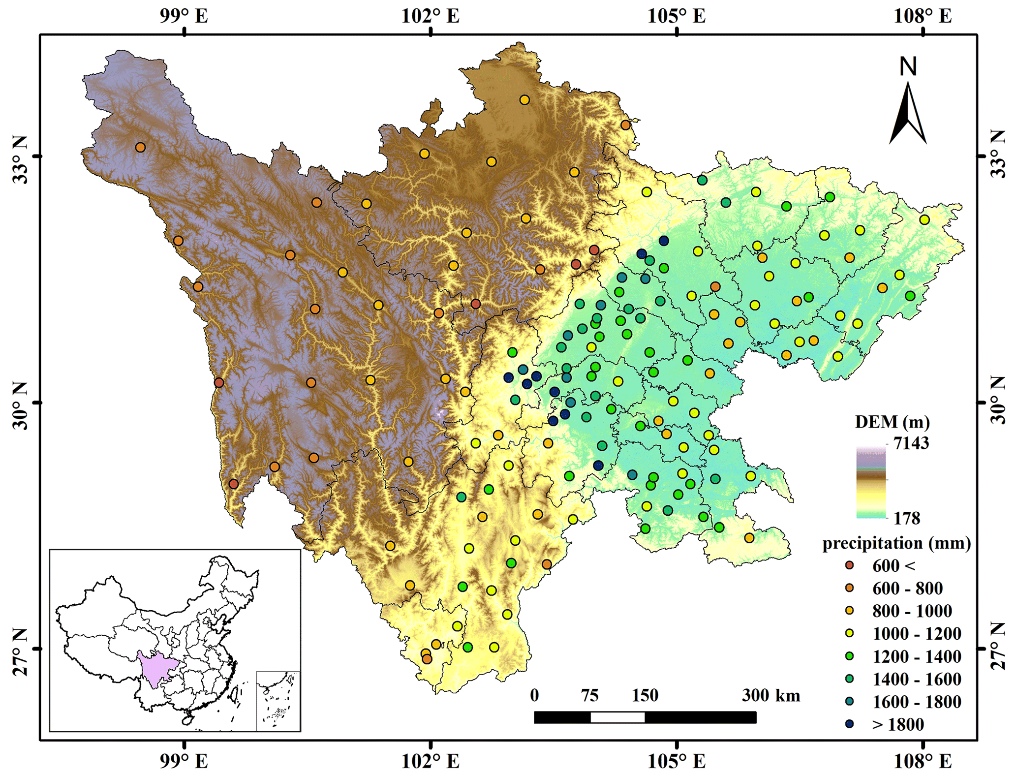
Figure 1Topography, rain gauges and geographic location of Sichuan Province in China.
2.2 Dataset
2.2.1 Rain gauge observations
The study region has 156 rain gauge stations, which shows an uneven distribution with high density in the east and low density in the west (Fig. 1). The average cover area of one rain gauge observation is about 3115 km2. Daily precipitation of all the stations for the period 2015–2019 was collected from the China Meteorological Data Service Center (CMDSC, 2021). The data quality was guaranteed based on some strict quality controls, such as manual inspection, outlier check and spatiotemporal consistency verification (Zhao and Yatagai, 2014). After that, the monthly precipitation was produced by aggregating the daily precipitation of rain gauges for each month.
2.2.2 Integrated MultisatellitE Retrievals for Global Precipitation Measurement (IMERG)
As the successor of TRMM, the National Aeronautics and Space Administration (NASA) and the Japan Aerospace Exploration Agency (JAXA) initiated the next-generation global precipitation observation mission (Hou et al., 2014). The IMERG products were generated by assimilating all microwave and infrared (IR) estimates, together with gauge observations (Huffman et al., 2019). It has the spatial resolution of 0.1∘ × 0.1∘ with the coverage from 60∘ S–60∘ N. IMERG provides three different products, including Early Run, Late Run and Final Run, which were estimated about 4 h, 14 h and 3.5 months after the observation time, respectively. Due to the incorporation of the Global Precipitation Climatology Centre (GPCC) rain gauge data, IMERG Final Run is more accurate than the others (Lu et al., 2019). Thus, the monthly IMERG V06B Final Run product was adopted in the study. It was downloaded from NASA (2021).
The average monthly precipitation of all rain gauges and that of IMERG at the corresponding grid cells from 2015–2019 over Sichuan Province are shown in Fig. 2. Obviously, IMERG has an overestimation in most months, and the wettest month is July 2018.
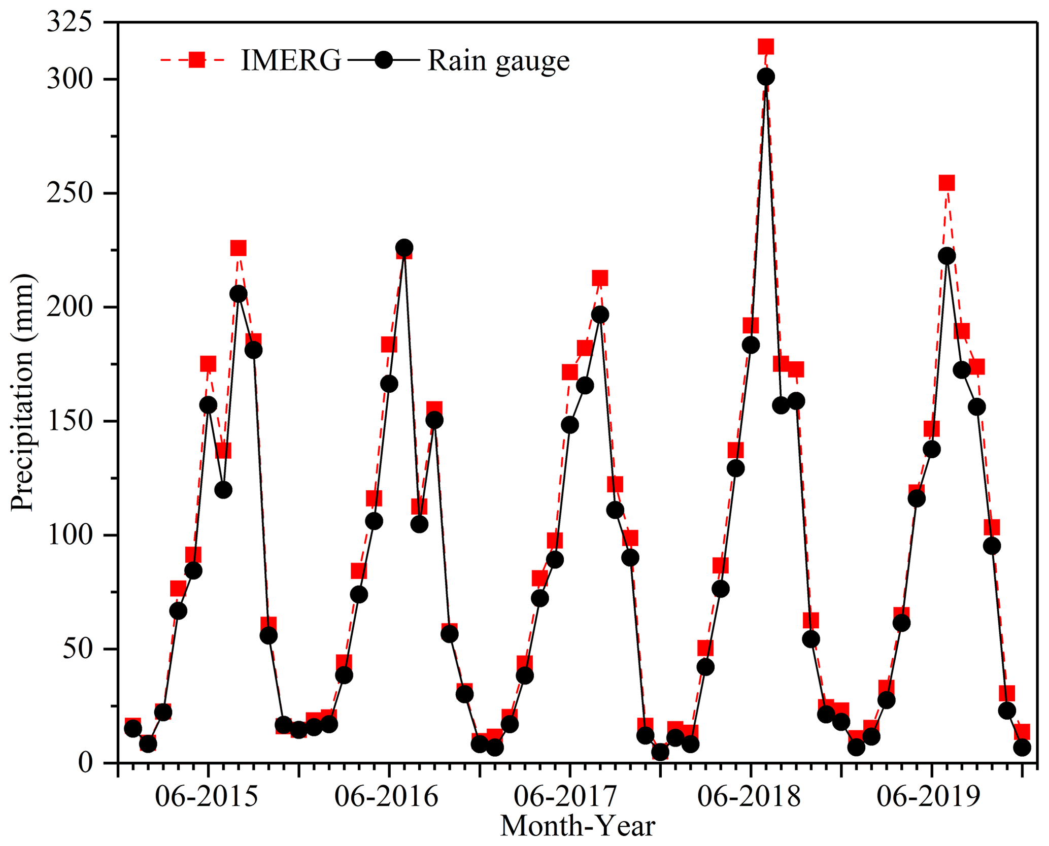
Figure 2Average monthly precipitation of all rain gauges and that of IMERG at the corresponding grid cells from 2015–2019 over Sichuan Province.
2.2.3 Environmental variables
Vegetation types have a significant impact on fluxes of sensible and latent heat into the atmosphere, apparently influencing the humidity of the lower atmosphere and further affecting moist convection (Spracklen et al., 2012). Therefore, as an indicator of vegetation activity, NDVI has been widely adopted to estimate precipitation (Wu et al., 2019; Immerzeel et al., 2009). In this study, the Moderate Resolution Imaging Spectroradiometer (MODIS) monthly NDVI with the resolution of 1 km (MOD13A3) from 2015 to 2019, NASA Earth Data (2021a) was used.
Precipitation can influence LST both in the daytime and at night; rain leads to cool temperatures, and droughts often couple with heat waves (Trenberth and Shea, 2005; Jing et al., 2016). Thus, the daytime LST (LSTD), nighttime LST (LSTN), and the difference between daytime and nighttime LSTs (LSTD−N) at a monthly scale were used in this study. Here, MODIS 8 d LST with a resolution of 1 km (MOD11A2) from 2015 to 2019 was downloaded from NASA Earth Data (2021b) and then temporally averaged into the monthly LST products.
Topography could affect the regional atmospheric circulation and the spatial pattern of precipitation through its thermal and dynamic forcing mechanisms (Jing et al., 2016; Jia et al., 2011). With the increase in elevations, the relative humidity of the air masses increases through expansion and cooling of the rising air masses, which brings precipitation (Jing et al., 2016). Thus, the precipitation–DEM relationship has been widely employed to downscale the satellite precipitation dataset. Here, the Shuttle Radar Topography Mission (SRTM) DEM (Shortridge and Messina, 2011) was used. The SRTM DEM with a spatial resolution of 90 m was downloaded from CGIAR (2021). and then resampled to 1 km by the pixel-averaging method. Since precipitation tends to be influenced by terrain variability and terrain orientation, DEM derivatives including slope, aspect and terrain relief (C. Chen et al., 2020; Yue et al., 2007) were also used in the study. These derivatives were extracted from the SRTM DEM using ArcGIS 10.3.
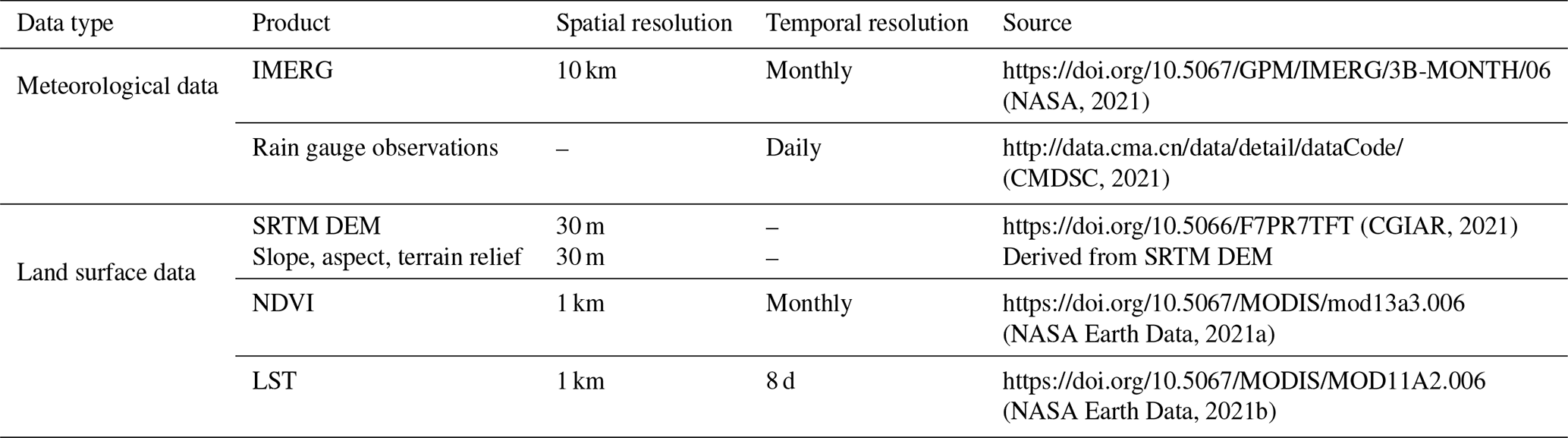
The detailed information of all the datasets used in the study is shown in Table 1.
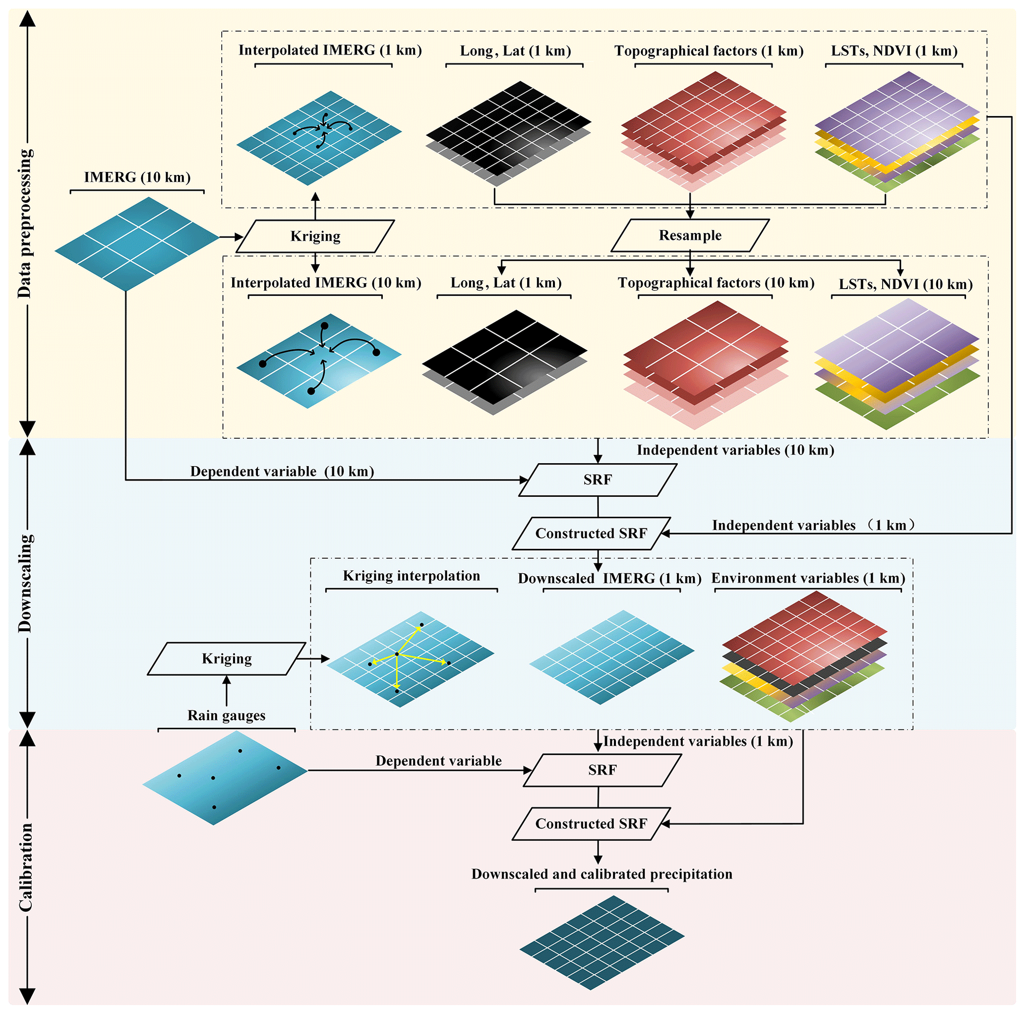
The flowchart of SRF-DC is illustrated in Fig. 3, which includes three stages: data processing, IMERG downscaling and downscaled IMERG calibration. It is noted that each IMERG pixel represents the areal average precipitation within it, whereas rain gauge measurements are point-based. Therefore, downscaling before calibration can decrease scale mismatch between pixel-based areal precipitation and gauge-based point measurements.
3.1 Random forest (RF)
The RF is an ensemble of several tree predictors such that each tree relies on a random and independent selection of some samples and features but with the same distribution (Breiman, 2001). The general framework of the RF is shown in Fig. 4. Specifically, each decision tree is constructed by randomly collecting some training data with a replacement, while the others are used to assess the tree performance (sample bagging). When constructing each tree, only a random subset of features is selected at each decision node (feature bagging). In the end, the majority vote for classification or the average prediction of all trees for regression is used to obtain the final output. Overall, the RF includes three parameters to set: number of trees, depth of the tree and number of features.
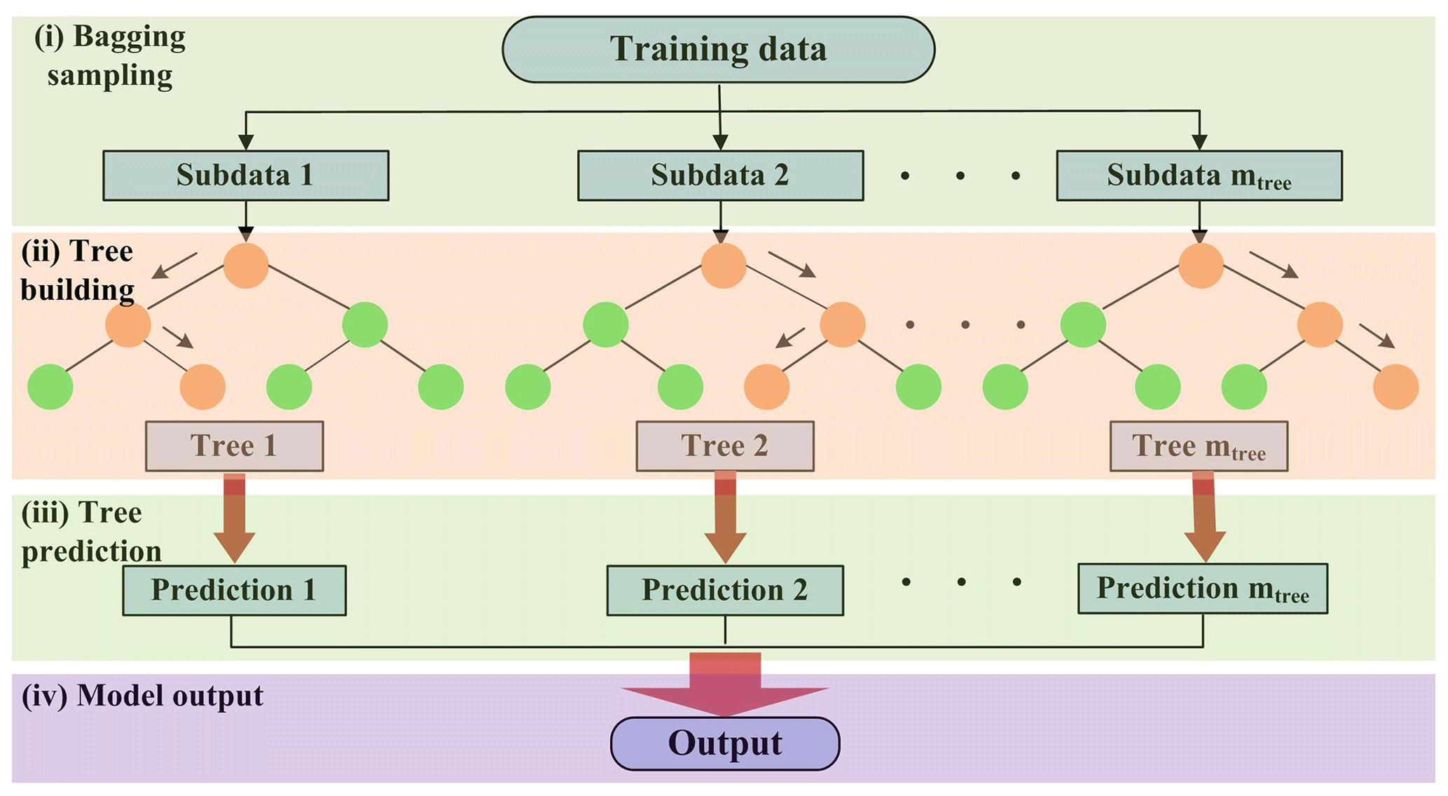
Meanwhile, the RF can evaluate the relative importance of each predictor by means of the out-of-bag (OOB) observations, i.e., the samples without being used for model construction (Breiman, 2001). Specifically, to measure the importance of the ith predictor, its values are permuted, while the values of the other predictors remain unchanged. Then, the OOB error based on the permuted samples is computed. Next, the importance score of the ith predictor is computed by averaging the difference between the OOB errors before and after the permutation. With the estimated scores, the importance of each variable is ranked.
In this study, the RF regression model was performed with the freely available codes, downloaded from the website https://code.google.com/archive/p/randomforest-matlab/downloads (last access: 10 March 2021).
3.2 Spatial random forest (SRF)
In essence, the classical RF is a non-spatial statistical technique for spatial prediction as it neglects sampling locations and general sampling pattern (Hengl et al., 2018). This can potentially cause sub-optimal estimations, especially when the spatial autocorrelation between dependent variables is high. To this end, a spatial RF (SRF) is proposed in this study. The general formulation of the SRF is as follows:
where p(s0) is the estimated precipitation at location s0; e is the fitting residual; f(⋅) is the function constructed by the SRF; and Xs and Xns are the spatial and non-spatial covariates, respectively.
In addition to spatial coordinates, one spatial covariate (Xs) is computed to account for the spatial autocorrelation of precipitation measurements between neighboring locations:
where si is the ith neighbor of s0, z(si) is the precipitation data of si, wi is its weight, and n is the number of neighbors.
In previous studies (Zhang et al., 2021; Li et al., 2017), the inverse distance weights (IDWs) were widely used. However, the IDW method only resorts to the spatial distance between the estimated location and its neighbor locations and does not consider the spatial autocorrelation between the neighbor locations. To overcome this limitation, an ordinary kriging (OK)-based variogram is adopted to estimate the interpolation weights in this study by solving the following linear system:
where μ is Lagrange parameter, and γ(⋅) is the semivariogram.
It can be concluded that the variogram-based weights consider the spatial autocorrelation not only between the known locations but also between the known locations and the interpolated location (Berndt and Haberlandt, 2018). In practice, the experimental semivariogram can be estimated from sample data as follows (Goovaerts, 2000):
where n is the number of data pairs with the attribute z separated by distance h.
To obtain the semivariogram at any h, a theoretical semivariogram model should be fitted to the experimental values. There are four commonly used theoretical semivariogram models: the spherical, Gaussian, exponential and power models. The best one with the best-fitting R2 was used in the study.
3.3 Working procedure of the proposed method
The detailed steps of SRF-DC are as follows (Fig. 3):
-
Each pixel value of the 10 km IMERG was re-estimated by OK interpolation with its k nearest neighbors (e.g., k=8) to obtain the interpolated IMERG (termed as ), the 10 km IMERG was interpolated by OK to obtain the interpolated 1 km IMERG (), and the gauge observations were interpolated by OK to produce the 1 km precipitation map (). This step aims to provide spatial variables for the SRF, i.e., Xs in Eq. (1). Since the semivariogram model cannot be accurately estimated from the sparse gauge measurements, the satellite-based precipitation was used to derive the model, as suggested by S. Chen et al. (2020). To estimate and , the raster-based 10 km IMERG was first transformed into the point-based form with spatial coordinates and precipitation values, and then the scattered points were interpolated by OK to produce raster-based maps.
-
The negative NDVI values were excluded from the original data, which mainly belong to snow and water bodies in the study site. The removed values were interpolated by OK with their neighbors to avoid information loss.
-
The 1 km environmental variables (i.e., NDVI, LSTD, LSTN, LSTD−N, DEM, slope, aspect, terrain relief, latitude and longitude) were resampled to 10 km resolution by the pixel-averaging method because the average value reflects the overall trend within each 10 km pixel and reduces the influence of outliers in the 1 km pixels.
-
The relationship between , and the original 10 km IMERG (D10 km) was constructed by the SRF:
where e is the fitting residual.
-
The 10 km IMERG (D10 km) was downscaled to 1 km (D1 km) by applying the constructed model in step (4) to and :
-
The relationship between the 1 km predictors and the gauge observations (G) was constructed by the SRF:
-
The 1 km precipitation data (C1 km) were produced based on the constructed relationship in step (6):
In this study, residual correction was ignored during downscaling and calibration as many previous studies (Karbalaye Ghorbanpour et al., 2021; Lu et al., 2019) demonstrated that residual correction on the ML-based technique could decrease prediction accuracy.
3.4 Comparative methods
In the study, the performance of SRF-DC was comparatively assessed in three ways. Firstly, we compared the results of SRF-DC with those of the classical methods including GWR, RF and a back propagation neural network (BPNN). Secondly, SRF-DC was compared with two frameworks: (i) the IMERG was first downscaled by the bilinear interpolation and then calibrated by the SRF (termed as Bi-SRF), and (ii) the IMERG was first downscaled by the SRF and then calibrated by GDA (termed as SRF-GDA). This could assess the significance of the SRF in both downscaling and calibration. Thirdly, SRF-DC at a monthly scale was compared with the annually based SRF fraction disaggregation method (termed as SRFdis). Specifically, the IMERG was first downscaled and calibrated by the SRF on an annual scale, and then the estimated annual precipitation was disaggregated into monthly precipitation using monthly fractions, as proposed by Duan and Bastiaanssen (2013). Finally, SRF-DC was compared with OK interpolation only on gauge measurements (termed as kriging). Overall, SRF-DC was compared with seven classical methods in this study including GWR, RF, BPNN, Bi-SRF, SRF-GDA, SRFdis and kriging.
To quantitatively analyze the performance of all the methods, all rain gauge observations were randomly divided into l folds (e.g., l=10), where the l−1 folds (i.e., training or validating data) were used to construct the model, while the remaining fold (i.e., testing data) was used to assess the performance of the model (Xu and Goodacre, 2018). During model construction, the l−1 folds were randomly divided into training and validating datasets with proportions of 80 % and 20 %, respectively, where the former was used to train the model and the latter to validate the model. Then, the performance of the model with the optimized parameters was assessed using the testing data. The aforementioned process was repeated l times until all folds were taken as the testing data.
3.5 Accuracy measures
We comparatively analyzed the performance of all methods with four accuracy measures including root mean square error (RMSE), mean error (ME), mean absolute error (MAE) and correlation coefficient (CC) (Jing et al., 2016; Sharifi et al., 2019). They are respectively expressed as follows:
where n is the number of testing points, and Ei andOi are the estimated and observed precipitation at location i, respectively.
Figure 5 illustrates the scatterplots between the predicted and observed precipitation on a monthly scale from 2015 to 2019. Results show that the original IMERG is heavily biased, with an ME value of 8.01 mm. In contrast, except for kriging, all the other models greatly reduce the bias, with ME values approximate to zero. In other words, the models with the incorporation of high-resolution variables become unbiased. With respect to RMSE, MAE and CC, BPNN produces worse results than the original IMERG. The performance of GWR is also unsatisfactory. This is mainly attributed to the complex relationship between precipitation and predictors, which cannot be properly described by the two models. The RF and kriging perform better than IMERG. The four SRF-based methods including SRF-DC, Bi-SRF, SRF-GDA and SRFdis outperform the other methods. This indicates the importance of spatial autocorrelation for precipitation estimation. Moreover, among the four versions of the SRF, SRF-GDA has the lowest accuracy, indicating that the SRF is more important for calibration than downscaling. SRF-DC with RMSE, MAE and CC values of 32.20 mm, 18.77 mm and 0.937 produces the best result. Thus, it can be concluded that (i) SRF-based downscaling and calibration are more effective than bilinear downscaling (Bi-SRF) and GDA-based calibration (SRF-GDA), and (ii) there is no obvious time latency for vegetation response to precipitation in the study site as SRF-DC on a monthly scale is slightly more accurate than SRFdis on an annual scale.
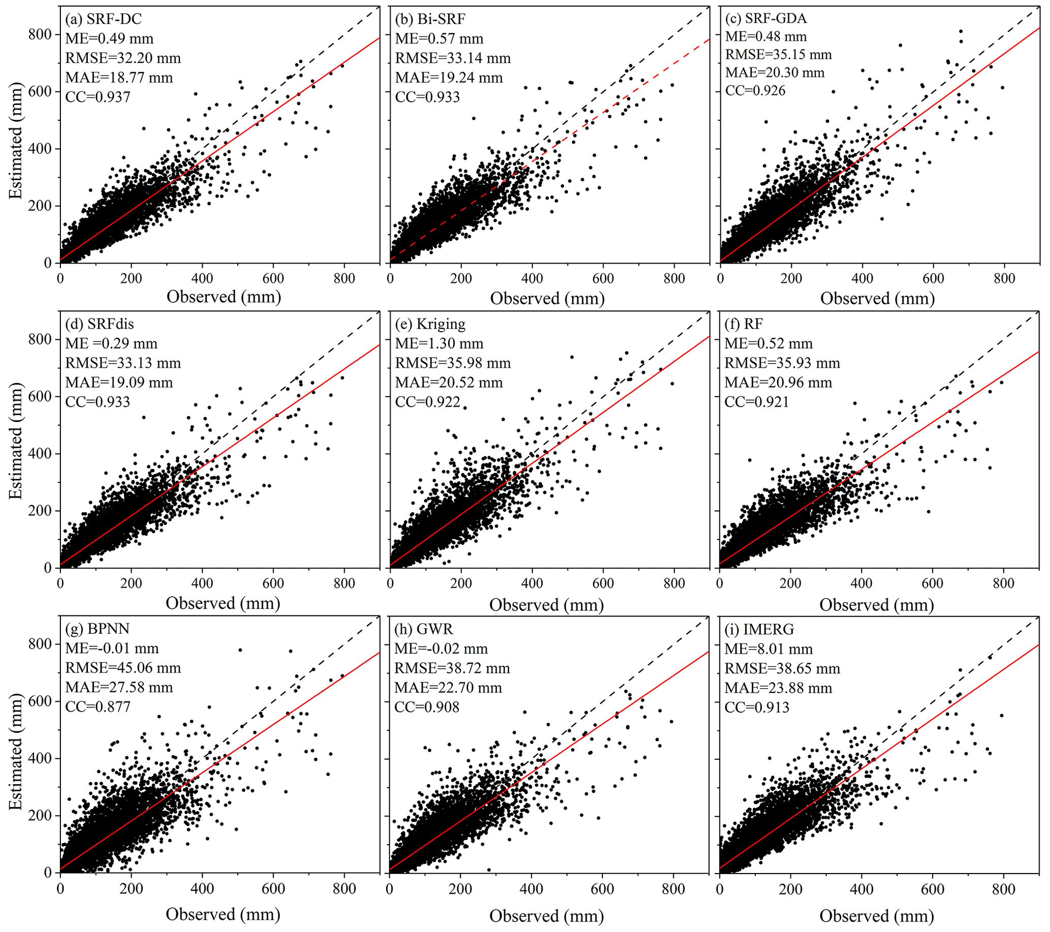
Figure 5Scatterplots between the estimated and observed precipitation on a monthly scale from 2015 to 2019. Fitting line with the red color models the relationship between the observed and estimated precipitation.
However, as shown in Fig. 5, all the methods significantly underestimate precipitation when the values are greater than 400 mm. To quantitatively analyze the performance of all methods on the high precipitation, their accuracy measures are shown in Table 2. Results show that all methods have poor results for these observations. A possible reason is that high precipitation is often caused by complicated environmental factors, which cannot be sufficiently explained by the constructed predictors–precipitation relationships. In terms of ME, SRF-GDA ranks the first, which is followed by kriging and SRF-DC. However, their ME values are less than −70 mm. With respect to RMSE and MAE, kriging performs the best, which is closely followed by SRF-DC, while with respect to CC, SRF-DC with a value of 0.64 outperforms the others.
Table 2Accuracy measures of all methods for estimating high precipitation (i.e., values greater than 400 mm).
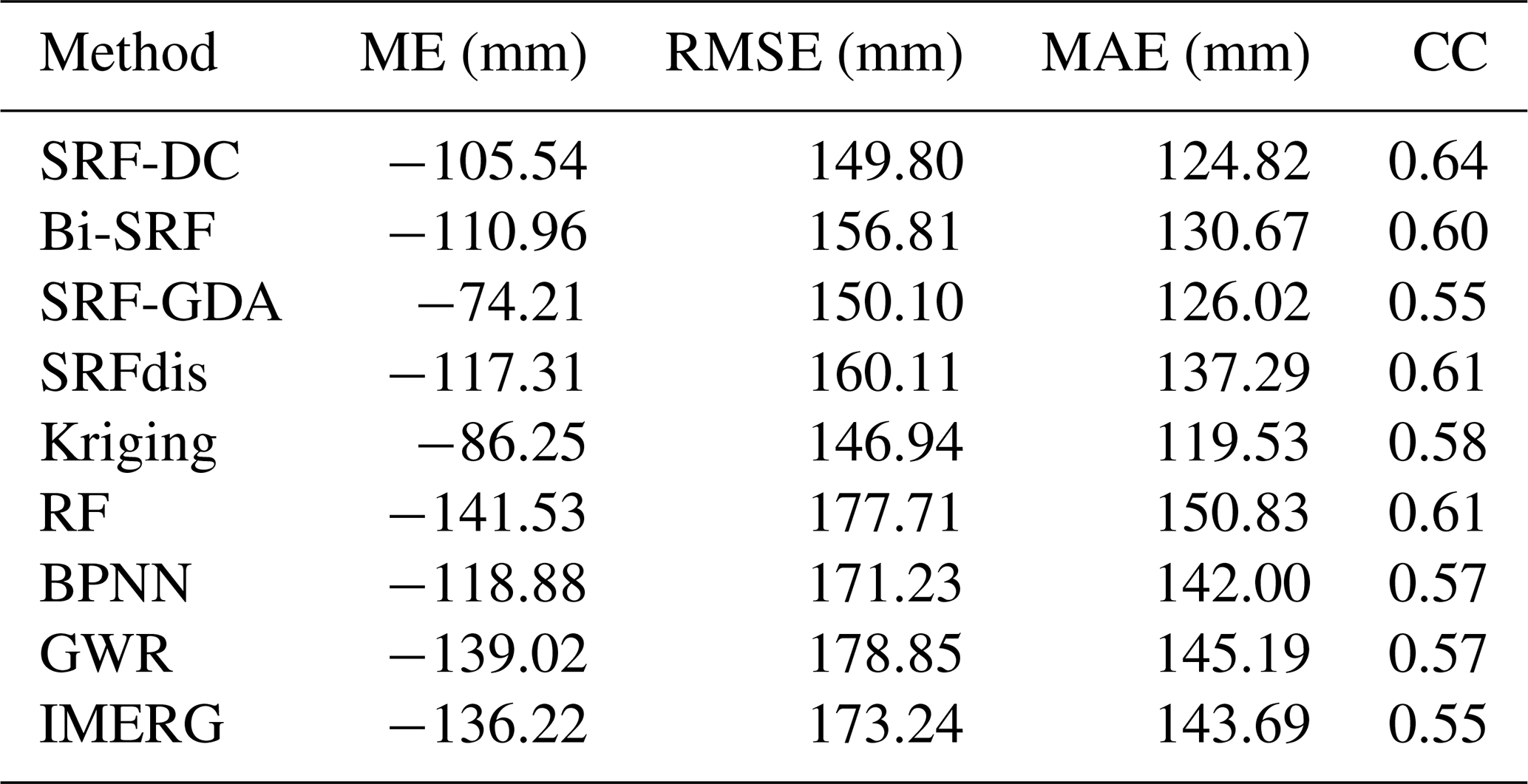
Figure 6 shows the boxplots of the four accuracy measures. Obviously, BPNN obtains the lowest accuracy. It is followed by GWR and IMERG. The RF and kriging show better results than BPNN, GWR and IMERG. The four methods based on the SRF seem more accurate than the classical methods. Moreover, SRF-DC slightly outperforms the other SRF-based methods, which highlights the benefit of including spatial autocorrelation for downscaling and calibration of satellite-based precipitation.
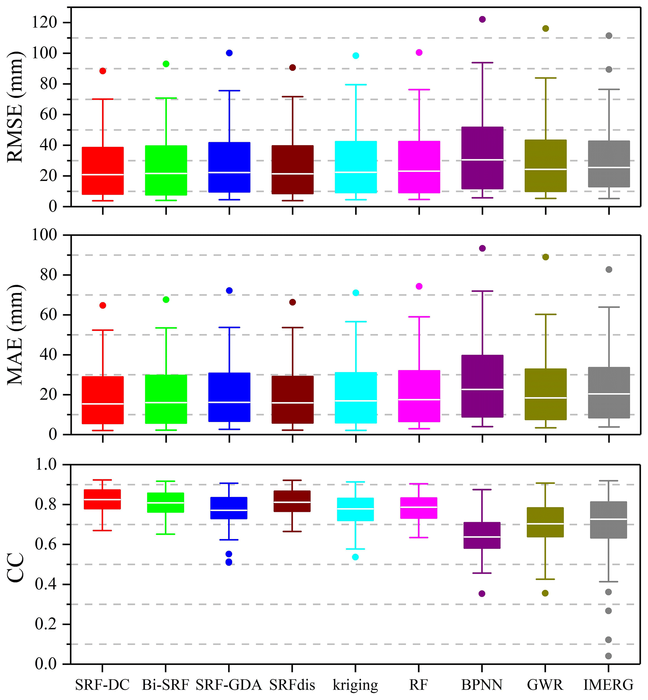
Figure 6Boxplots of RMSE, MAE and CC values of all the methods on a monthly scale during 2015–2019.
Figure 7 shows the RMSE spatial distributions of SRF-DC, SRFdis, RF, BPNN, kriging and GWR on all gauge stations. Overall, the RMSEs tend to be larger in the middle area since it has higher precipitation than the other areas (Fig. 1). BPNN (Fig. 7d) yields the poorest result, where many stations have RMSE values greater than 60 mm. It is followed by GWR (Fig. 7f). The RF (Fig. 7c) and kriging (Fig. 7e) are better than GWR and BPNN at most stations. SRF-DC (Fig. 7a) and SRFdis (Fig. 7b) are more accurate than the classical methods, especially at the stations in the middle area.
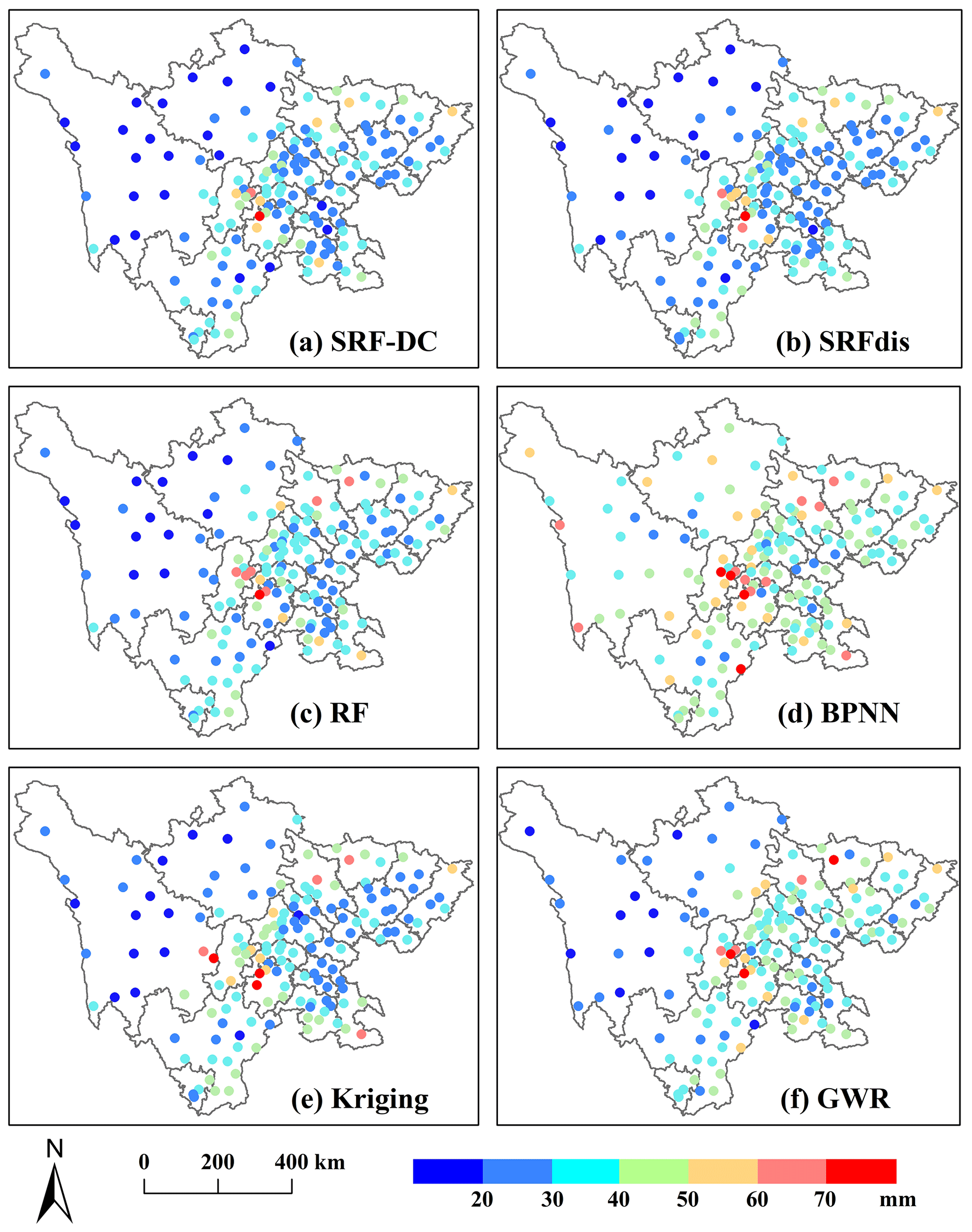
Figure 7RMSE distributions of SRF-DC and some representative methods for all gauge stations on a monthly scale during 2015–2019.
Since the wettest month is July 2018 (Fig. 2), it is taken as an example to show the precipitation maps of SRF-DC and some classical methods. Moreover, the semivariogram of kriging derived from the original IMERG and its prediction error map are shown since they play an important role in the performance of kriging and SRF-based methods. Results (Fig. 8) indicate that precipitation produced by all the methods have spatial distribution patterns similar to IMERG, with much high precipitation in the middle and low precipitation in the east. The ML-based methods have more spatial details of precipitation than IMERG due to the inclusion of high-resolution predictors for precipitation estimation. The kriging map is so smooth that many details and variations in precipitation pattern are lost. This is expected as it only uses ground measurements for the interpolation. The RF shows obvious unnatural discontinuities at the bottom. GWR suffers from systematic anomalies, with values clearly greater than their neighbors. In comparison, SRF-DC produces a good precipitation map.
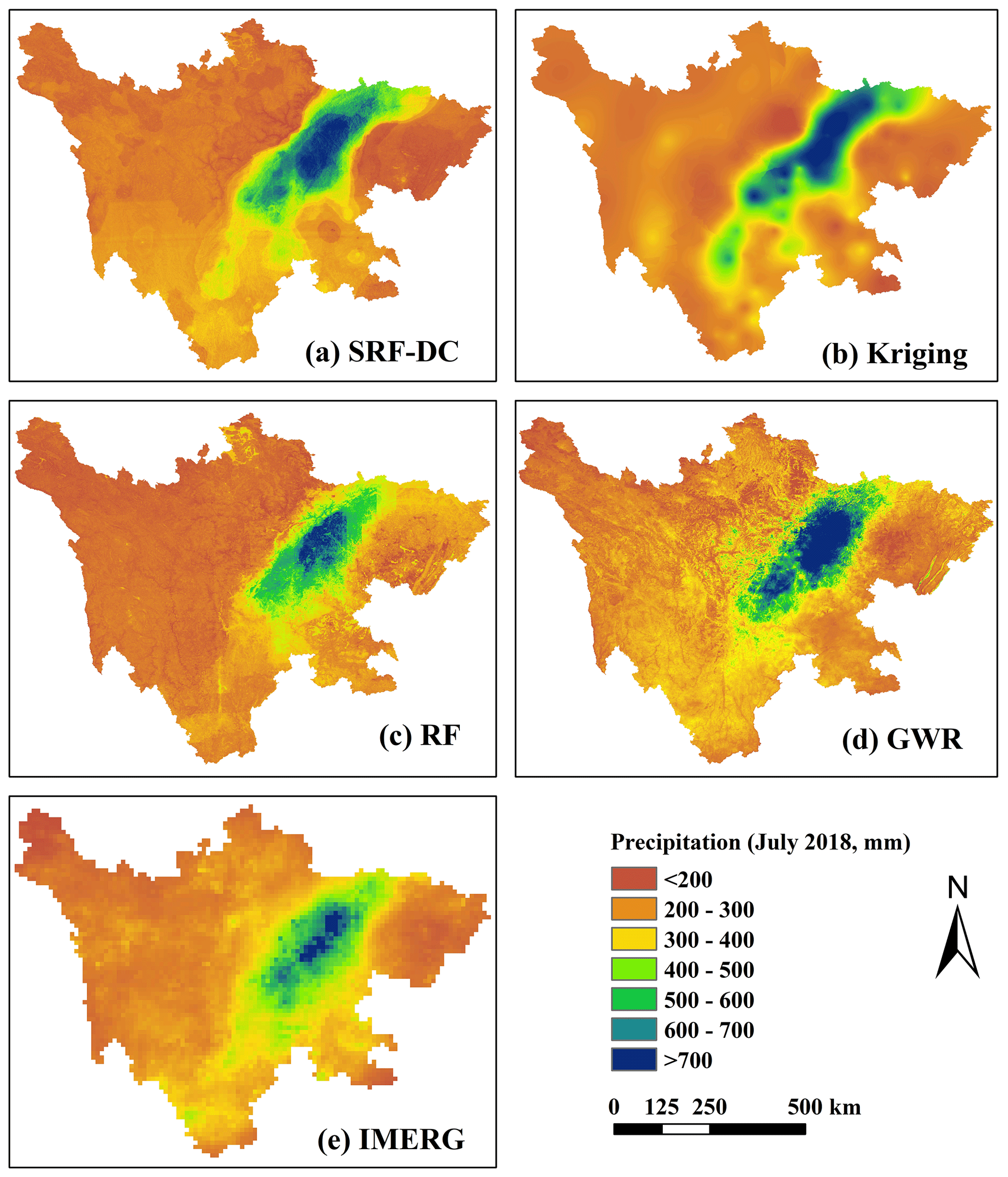
Figure 8Downscaled and calibrated precipitation maps of SRF-DC and some representative methods in the wettest month (July 2018).
The semivariogram and prediction error map of OK are shown in Fig. 9. Obviously, OK has a spherical model with a nugget variance (C0) of 10.0 m2, sill (C0+C) of 10 560 m2, residual sum of squares (Rss) of 8 800 611 m2, range (A0) of 321,000 m and fitting R2 of 0.962, respectively (Fig. 9a). The prediction error map (Fig. 9b) illustrates that the errors in the west are larger than in the east and in the boundary are larger than in the interior. It can be inferred that large errors are mainly located in the areas with a sparse distribution of rain gauges. Moreover, the error magnitudes are not related to RMSE distribution (Fig. 7) and precipitation pattern (Fig. 8).
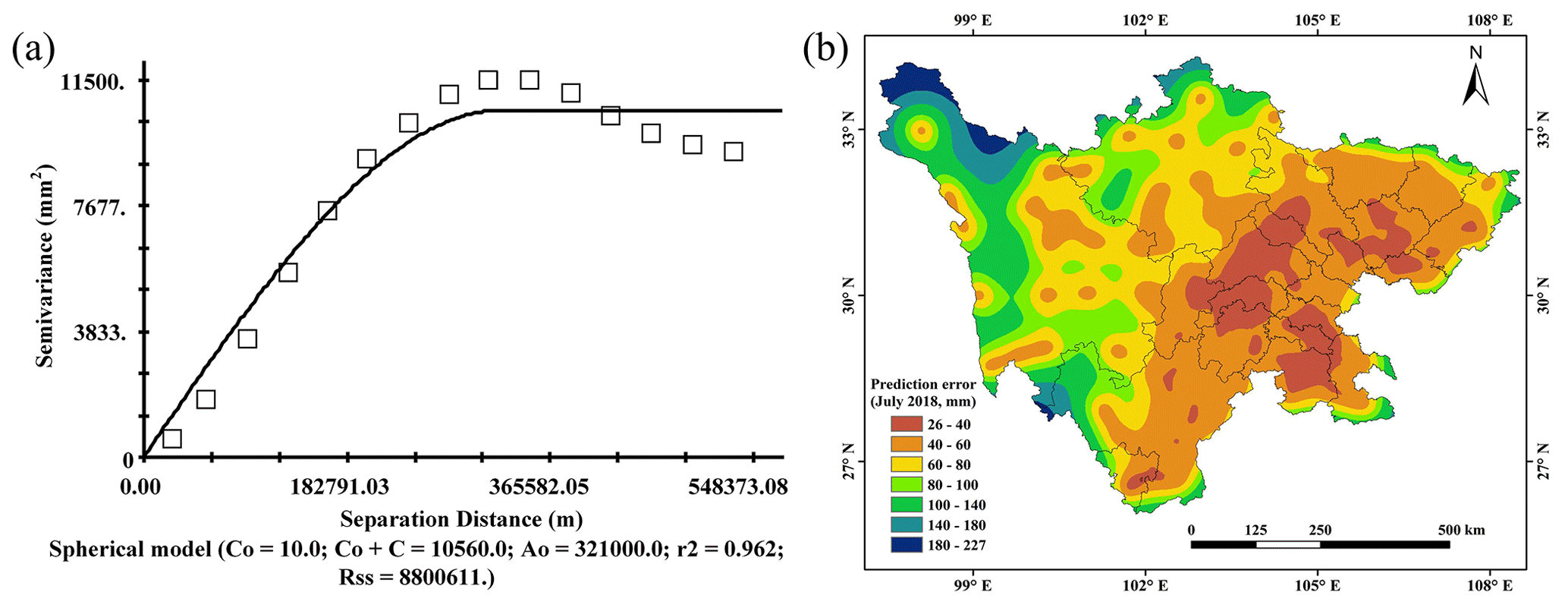
Figure 9(a) Semivariogram, (b) prediction error. Semivariogram and prediction error map of kriging in the wettest month (July 2018).
For downscaling and calibration of satellite-based precipitation, the three most important factors for constructing predictors–precipitation relationships are model, predictor and temporal scale (F. Chen et al., 2020). Thus, they should be carefully selected to produce accurate precipitation data.
5.1 Model
In previous studies, the most commonly adopted model was GWR (Xu et al., 2015; Chen et al., 2015; Zhao et al., 2018) since it considers the spatial variation between the predictors and precipitation. However, we found that due to the sparse distribution of rain gauge stations (Lu et al., 2019), GWR produced worse results than the original IMERG in the study region. The RF and kriging outperformed GWR. Nevertheless, the two methods have some shortcomings. For example, the precipitation map of kriging was so smooth that many details were lost, and the RF did not consider the spatial autocorrelation of precipitation measurements. In comparison, SRF-based methods with the consideration of spatial autocorrelation information demonstrated higher accuracy than the classical methods. Moreover, SRF-DC yielded slightly better results than Bi-SRF, SRF-GDA and SRFdis.
5.2 Environmental predictors
NDVI, latitude, longitude and DEM-based parameters were commonly adopted as predictors to estimate precipitation (Shi et al., 2015). However, satellite-based precipitation across regions with no relationship with NDVI could not be estimated, such as in barren or snow areas (Xu et al., 2015). Jing et al. (2016) indicated that the downscaled models including LST features (LSTs) performed better than those without LSTs. Thus, in addition to NDVI and DEM-related parameters, daytime LST (LSTD), nighttime LST (LSTN), and difference-between-day-and-night LSTs (LSTD−N) were used in this study.
Based on the RF, the relative importance of each predictor (i.e., predictor importance estimate) is shown in Fig. 10. Obviously, precipitation from kriging interpolation has the most importance. This is because the interpolated value is directly related to precipitation. Kriging estimation is followed by the downscaled precipitation. Longitude is the third most important variable, which is followed by latitude. This result is consistent with that of Karbalaye Ghorbanpour et al. (2021). They indicated that compared to NDVI, LST and DEM, longitude ranks first with respect to importance score.
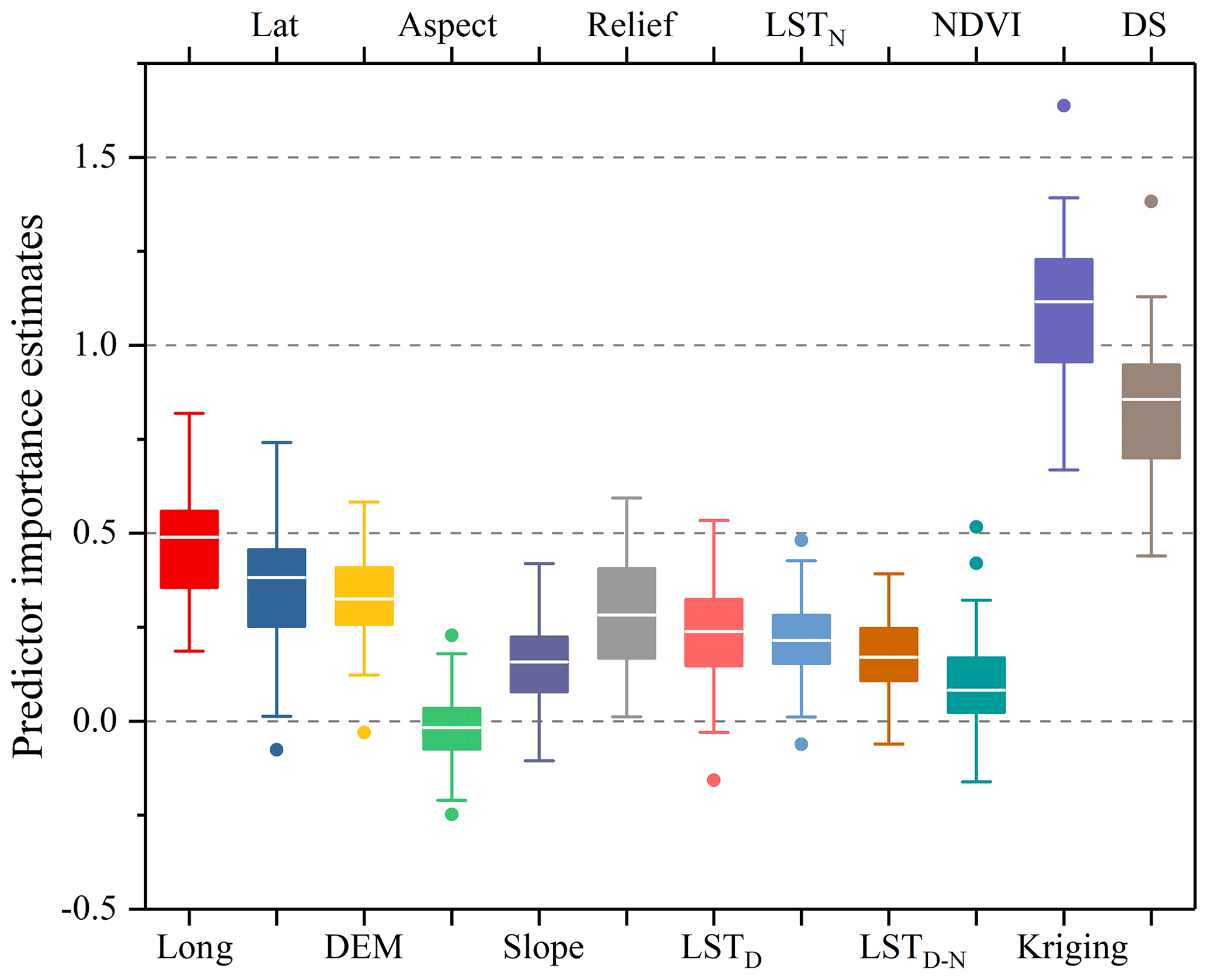
Figure 10Predictor importance estimates (lat: latitude; long: longitude; DS: downscaled precipitation).
The three LSTs also have a great impact on the precipitation estimation, where LSTD seems slightly more important than LSTN and LSTD−N. NDVI has a slight effect on the precipitation, which ranks second to last. This might be due to the fact that NDVI is influenced by both precipitation and temperature at the study site, and the low temperature above certain elevations hinders the vegetation growth. It is less likely that the response of vegetation to precipitation has the delay since SRF-DC on a monthly scale is more accurate than SRFdis on an annual scale.
Among the 12 predictors, aspect has the least importance. This conclusion was also obtained by Ma et al. (2017) for downscaling TMPA 3B43 V7 data over the Tibet Plateau. DEM, terrain relief and slope seem more important than aspect since precipitation is closely related to topography (Jing et al., 2016). The results are consistent with previous studies (Immerzeel et al., 2009; Jing et al., 2016).
5.3 Temporal scale
Temporal scale has a great effect on the selection of predictors for precipitation estimation. There is a debate on whether NDVI should be taken as a predictor for downscaling and calibration of monthly precipitation. Some (Duan and Bastiaanssen, 2013; Immerzeel et al., 2009) argued that NDVI could not be used for monthly precipitation estimation since the response of NDVI to precipitation was usually delayed by 2 or 3 months. However, some (Brunsell, 2006; Xu et al., 2015; Lu et al., 2019; S. Chen et al., 2020) stated that the precipitation–NDVI relationship was hardly time-delayed since vegetation could influence precipitation by adjusting temperature and air moisture during the growing seasons. Thus, it was possible to estimate precipitation with NDVI at a monthly scale. In this study, it was found that SRF-DC on a monthly scale was slightly more accurate than that on an annual scale (i.e., SRFdis). This indicates that the response of vegetation to precipitation has no obvious time delay, and NDVI can be used for monthly precipitation estimates.
5.4 Easy-to-use feature
Since the classical RF did not consider the spatial information in the modeling process, Hengl et al. (2018) proposed an improved RF for spatial estimation, where the buffer distances between the estimated location and measured locations were taken as the predictors. Motivated by this idea, Baez-Villanueva et al. (2020) presented an RF-based method (RF-MEP) for merging satellite precipitation products and rain gauge measurements, where the spatial distances from all rain gauges to the grid cells in the study site were used as the variables. However, as stated by Baez-Villanueva et al. (2020), RF-MEP has a huge computational cost since the number of extra input features equals that of gauge measurements. Moreover, RF-MEP ignores the spatial autocorrelation of precipitation between neighboring locations. In comparison, the SRF only requires one extra feature that is estimated by kriging interpolation on the precipitation measurements. Thus, compared to the buffer distance layers-based RF, the SRF is highly effective. Moreover, with the variogram-based kriging interpolation, the spatial autocorrelation of precipitation not only between the gauge locations but also between the estimated location and gauge locations is taken into account. Thus, the SRF has the merits of accuracy, effectivity and ease of use.
5.5 Limitations and further research
Although SRF-DC shows more promising results than the classical methods, it still suffers from some limitations, which should be solved in our further research. Firstly, SRF-DC is more complex than Bi-SRF and SRF-GDA since the SRF is used in both downscaling and calibration. Yet, applying the SRF to downscale IMERG might not be prerequisite since SRF-DC is only slightly better than Bi-SRF. However, the SRF should be used to calibrate IMERG due to the much higher accuracy of SRF-DC than SRF-GDA. Secondly, SRF-DC has low accuracy on high precipitation (e.g., >400 mm) since extreme precipitation is often caused by unpredictable factors. Thus, other available variables such as soil moisture (Fan et al., 2019; Brocca et al., 2019) and meteorological conditions such as cloud properties (Sharifi et al., 2019) could be adopted to further improve IMERG quality. Thirdly, the correction of satellite-based precipitation on higher temporal scales (e.g., daily or hourly) is challenging (Wu et al., 2020; F. Chen et al., 2020; Lima et al., 2021; Sun and Lan, 2021; Yan et al., 2021) since the relationships between environmental variables and precipitation on these scales are far less evident and difficult to capture. Although SRF-DC is general, its performance on these scales should be further assessed. Finally, numerous satellite-based precipitation products have been available, and each one has its shortcomings and advantages for the capture of spatial precipitation patterns (S. Chen et al., 2020; Baez-Villanueva et al., 2020). Thus, the fusion of multiple precipitation products based on SRF-DC is an alternative to improve the quality of precipitation data.
To enhance the resolution (from 0.1∘ to 1 km) and accuracy of the monthly IMERG V06B Final Run product, a spatial RF (SRF)-based downscaling and calibration method (SRF-DC) was proposed in this study. The performance of SRF-DC was compared with those of seven methods including GWR, RF, BPNN, Bi-SRF, SRF-GDA, SRFdis and kriging on monthly IMERG from 2015 to 2019 over Sichuan Province, China. The main findings and conclusions can be summarized as follows:
-
The SRF-based methods including SRF-DC, Bi-SRF, SRF-GDA and SRFdis were more accurate than the classical methods. Moreover, SRF-DC performed slightly better than Bi-SRF and SRF-GDA.
-
The comparison between the monthly based and annually based estimation demonstrated that there was no statistically significant difference between them, indicating that NDVI could be used for monthly precipitation estimation at the study site.
-
Kriging outperformed the original IMERG, BPNN and GWR in terms of RMSE, MAE and CC. However, its interpolation map suffered from the serious loss of spatial precipitation patterns.
-
Based on the variable-importance assessment of the RF, the precipitation interpolated by kriging on the gauge measurements was the most important variable, while terrain aspect was the least important. This indicated that considering spatial autocorrelation was beneficial for precipitation estimation.
Overall, SRF-DC is general, robust, accurate and easy to use as it shows promising results in the study area with heterogeneous terrain morphology and precipitation. Thus, it can be easily applied to other regions, where precipitation data with high resolution and high accuracy are urgently required.
The gauge data are from the China Meteorological Data Service Center (http://data.cma.cn/data/detail/dataCode/SURF_CLI_CHN_MUL_DAY_CES_V3.0.html, CMDSC, 2021). The GPM data are from https://doi.org/10.5067/GPM/IMERG/3B-MONTH/06 (NASA, 2021). The SRTM data are from https://doi.org/10.5066/F7PR7TFT (CGIAR, 2021). The MOD13A3 data are from https://doi.org/10.5067/MODIS/mod13a3.006 (NASA Earth Data, 2021a). The MOD11A2 data are from https://doi.org/10.5067/MODIS/MOD11A2.006 (NASA Earth Data 2021b).
CF and YY conceived the idea and acquired the project and financial support. BJ conducted the detailed analysis. CF contributed to the writing and revisions.
The contact author has declared that neither they nor their co-authors have any competing interests.
Publisher's note: Copernicus Publications remains neutral with regard to jurisdictional claims in published maps and institutional affiliations.
This article is part of the special issue “Experiments in Hydrology and Hydraulics”. It is not associated with a conference.
This work was supported by the National Natural Science Foundation of China (grant no. 41804001), the Shandong Provincial Natural Science Foundation of China (grant nos. ZR2020YQ26, ZR2019MD007, ZR2019BD006), a project of the Shandong Province Higher Educational Youth Innovation Science and Technology Program (grant no. 2019KJH007), the Shandong Provincial Key Research and Development Program (Major Scientific and Technological Innovation Project) (grant no. 2019JZZY010429), and the Scientific Research Foundation of Shandong University of Science and Technology for Recruited Talents (grant no. 2019RCJJ003).
This paper was edited by Carla Ferreira and reviewed by Priscilla Minotti, Eric Gaume and two anonymous referees.
Ashouri, H., Hsu, K.-L., Sorooshian, S., Braithwaite, D. K., Knapp, K. R., Cecil, L. D., Nelson, B. R., and Prat, O. P.: PERSIANN-CDR: Daily Precipitation Climate Data Record from Multisatellite Observations for Hydrological and Climate Studies, B. Am. Meteorol. Soc., 96, 69–83, https://doi.org/10.1175/bams-d-13-00068.1, 2015.
Baez-Villanueva, O. M., Zambrano-Bigiarini, M., Beck, H. E., McNamara, I., Ribbe, L., Nauditt, A., Birkel, C., Verbist, K., Giraldo-Osorio, J. D., and Xuan Thinh, N.: RF-MEP: A novel Random Forest method for merging gridded precipitation products and ground-based measurements, Remote Sens. Environ., 239, 111606, https://doi.org/10.1016/j.rse.2019.111606, 2020.
Beck, H. E., van Dijk, A. I. J. M., Levizzani, V., Schellekens, J., Miralles, D. G., Martens, B., and de Roo, A.: MSWEP: 3-hourly 0.25∘ global gridded precipitation (1979–2015) by merging gauge, satellite, and reanalysis data, Hydrol. Earth Syst. Sci., 21, 589–615, https://doi.org/10.5194/hess-21-589-2017, 2017.
Beck, H. E., Wood, E. F., Pan, M., Fisher, C. K., Miralles, D. G., van Dijk, A. I. J. M., McVicar, T. R., and Adler, R. F.: MSWEP V2 Global 3-hourly 0.1∘ Precipitation: Methodology and Quantitative Assessment, B. Am. Meteorol. Soc., 100, 473–500, https://doi.org/10.1175/bams-d-17-0138.1, 2019.
Belgiu, M., Drăgu, L. J. I. J. o. P., and Sensing, R.: Random forest in remote sensing: A review of applications and future directions, ISPRS J. Photogramm. Remote Sens., 114, 24–31, https://doi.org/10.1016/j.isprsjprs.2016.01.011, 2016.
Berndt, C. and Haberlandt, U.: Spatial interpolation of climate variables in Northern Germany-Influence of temporal resolution and network density, Journal of Hydrology-Regional Studies, 15, 184–202, https://doi.org/10.1016/j.ejrh.2018.02.002, 2018.
Berndt, C., Rabiei, E., and Haberlandt, U.: Geostatistical merging of rain gauge and radar data for high temporal resolutions and various station density scenarios, J. Hydrol., 508, 88–101, https://doi.org/10.1016/j.jhydrol.2013.10.028, 2014.
Bhuiyan, M. A. E., Nikolopoulos, E. I., Anagnostou, E. N., Quintana-Seguí, P., and Barella-Ortiz, A.: A nonparametric statistical technique for combining global precipitation datasets: development and hydrological evaluation over the Iberian Peninsula, Hydrol. Earth Syst. Sci., 22, 1371–1389, https://doi.org/10.5194/hess-22-1371-2018, 2018.
Breiman, L.: Random Forests, Machine Learning, 45, 5–32, 2001.
Brocca, L., Filippucci, P., Hahn, S., Ciabatta, L., Massari, C., Camici, S., Schüller, L., Bojkov, B., and Wagner, W.: SM2RAIN–ASCAT (2007–2018): global daily satellite rainfall data from ASCAT soil moisture observations, Earth Syst. Sci. Data, 11, 1583–1601, https://doi.org/10.5194/essd-11-1583-2019, 2019.
Brunsell, N. A.: Characterization of land-surface precipitation feedback regimes with remote sensing, Remote Sens. Environ., 100, 200–211, https://doi.org/10.1016/j.rse.2005.10.025, 2006.
CGIAR: SRTM Data, CGIAR [data set], https://doi.org/10.5066/F7PR7TFT, 2021.
Chao, L., Zhang, K., Li, Z., Zhu, Y., Wang, J., and Yu, Z.: Geographically weighted regression based methods for merging satellite and gauge precipitation, J. Hydrol., 558, 275–289, https://doi.org/10.1016/j.jhydrol.2018.01.042, 2018.
Cheema, M. J. M. and Bastiaanssen, W. G. M.: Local calibration of remotely sensed rainfall from the TRMM satellite for different periods and spatial scales in the Indus Basin, Int. J. Remote Sens., 33, 2603–2627, https://doi.org/10.1080/01431161.2011.617397, 2012.
Chen, C., Zhao, S., Duan, Z., and Qin, Z.: An Improved Spatial Downscaling Procedure for TRMM 3B43 Precipitation Product Using Geographically Weighted Regression, IEEE J. Sel. Top. Appl., 8, 4592–4604, https://doi.org/10.1109/JSTARS.2015.2441734, 2015.
Chen, C., Yang, S., and Li, Y.: Accuracy Assessment and Correction of SRTM DEM using ICESat/GLAS Data under Data Coregistration, Remote Sens., 12, 3435, https://doi.org/10.3390/rs12203435, 2020.
Chen, F., Liu, Y., Liu, Q., and Li, X.: Spatial downscaling of TRMM 3B43 precipitation considering spatial heterogeneity, Int. J. Remote Sens., 35, 3074–3093, https://doi.org/10.1080/01431161.2014.902550, 2014.
Chen, F., Gao, Y., Wang, Y., and Li, X.: A downscaling-merging method for high-resolution daily precipitation estimation, J. Hydrol., 581, 124414, https://doi.org/10.1016/j.jhydrol.2019.124414, 2020.
Chen, J., Brissette, F. P., Chaumont, D., and Braun, M.: Finding appropriate bias correction methods in downscaling precipitation for hydrologic impact studies over North America, Water Resour. Res., 49, 4187–4205, https://doi.org/10.1002/wrcr.20331, 2013.
Chen, S., Xiong, L., Ma, Q., Kim, J.-S., Chen, J., and Xu, C.-Y.: Improving daily spatial precipitation estimates by merging gauge observation with multiple satellite-based precipitation products based on the geographically weighted ridge regression method, J. Hydrol., 589, 125156, https://doi.org/10.1016/j.jhydrol.2020.125156, 2020.
Chen, S.-T., Yu, P.-S., and Tang, Y.-H.: Statistical downscaling of daily precipitation using support vector machines and multivariate analysis, J. Hydrol., 385, 13–22, https://doi.org/10.1016/j.jhydrol.2010.01.021, 2010.
Chen, Y., Huang, J., Sheng, S., Mansaray, L. R., Liu, Z., Wu, H., and Wang, X.: A new downscaling-integration framework for high-resolution monthly precipitation estimates: Combining rain gauge observations, satellite-derived precipitation data and geographical ancillary data, Remote Sens. Environ., 214, 154–172, https://doi.org/10.1016/j.rse.2018.05.021, 2018.
CMDSC: China Meteorological Data Service Center: Gauge data [data set], available at: http://data.cma.cn/data/detail/dataCode/SURF_CLI_CHN_MUL_DAY_CES_V3.0.html, last access: 10 March 2021.
Duan, Z. and Bastiaanssen, W. G. M.: First results from Version 7 TRMM 3B43 precipitation product in combination with a new downscaling–calibration procedure, Remote Sens. Environ., 131, 1–13, https://doi.org/10.1016/j.rse.2012.12.002, 2013.
Elnashar, A., Zeng, H., Wu, B., Zhang, N., Tian, F., Zhang, M., Zhu, W., Yan, N., Chen, Z., Sun, Z., Wu, X., and Li, Y.: Downscaling TRMM Monthly Precipitation Using Google Earth Engine and Google Cloud Computing, Remote Sens., 12, 3860, https://doi.org/10.3390/rs12233860, 2020.
Fan, D., Wu, H., Dong, G., Jiang, X., and Xue, H.: A Temporal Disaggregation Approach for TRMM Monthly Precipitation Products Using AMSR2 Soil Moisture Data, Remote Sens., 11, 2962, https://doi.org/10.3390/rs11242962, 2019.
Funk, C., Peterson, P., Landsfeld, M., Pedreros, D., Verdin, J., Shukla, S., Husak, G., Rowland, J., Harrison, L., Hoell, A., and Michaelsen, J.: The climate hazards infrared precipitation with stations – a new environmental record for monitoring extremes, Scientific Data, 2, 150066, doi:10.1038/sdata.2015.66, 2015.
Gebregiorgis, A. S. and Hossain, F.: Understanding the Dependence of Satellite Rainfall Uncertainty on Topography and Climate for Hydrologic Model Simulation, IEEE T. Geosci. Remote, 51, 704–718, https://doi.org/10.1109/TGRS.2012.2196282, 2013.
Goovaerts, P.: Geostatistical approaches for incorporating elevation into the spatial interpolation of rainfall, J. Hydrol., 228, 113–129, 2000.
Haile, A. T., Habib, E., and Rientjes, T.: Evaluation of the climate prediction center (CPC) morphing technique (CMORPH) rainfall product on hourly time scales over the source of the Blue Nile River, Hydrol. Process., 27, 1829–1839, https://doi.org/10.1002/hyp.9330, 2013.
Hengl, T., Nussbaum, M., Wright, M. N., Heuvelink, G. B., and Gräler, B. J. P.: Random forest as a generic framework for predictive modeling of spatial and spatio-temporal variables, PeerJ, 6, e5518, https://doi.org/10.7717/peerj.5518, 2018.
Hou, A. Y., Kakar, R. K., Neeck, S., Azarbarzin, A. A., Kummerow, C. D., Kojima, M., Oki, R., Nakamura, K., and Iguchi, T.: The Global Precipitation Measurement Mission, B. Am. Meteorol. Soc., 95, 701–722, https://doi.org/10.1175/bams-d-13-00164.1, 2014.
Huffman, G., Bolvin, D., Braithwaite, D., Hsu, K., and Joyce, R.: Algorithm theoretical basis document (ATBD) NASA global precipitation measurement (GPM) integrated multi-satellitE Retrievals for GPM (IMERG), Nasa, 29 December 2019.
Huffman, G. J., Bolvin, D. T., Nelkin, E. J., Wolff, D. B., Adler, R. F., Gu, G., Hong, Y., Bowman, K. P., and Stocker, E. F.: The TRMM Multisatellite Precipitation Analysis (TMPA): Quasi-Global, Multiyear, Combined-Sensor Precipitation Estimates at Fine Scales, J. Hydrometeorol., 8, 38–55, https://doi.org/10.1175/jhm560.1, 2007.
Immerzeel, W. W., Rutten, M. M., and Droogers, P.: Spatial downscaling of TRMM precipitation using vegetative response on the Iberian Peninsula, Remote Sens. Environ., 113, 362–370, https://doi.org/10.1016/j.rse.2008.10.004, 2009.
Jia, S., Zhu, W., Lű, A., and Yan, T.: A statistical spatial downscaling algorithm of TRMM precipitation based on NDVI and DEM in the Qaidam Basin of China, Remote Sens. Environ., 115, 3069–3079, https://doi.org/10.1016/J.RSE.2011.06.009, 2011.
Jing, W., Yang, Y., Yue, X., and Zhao, X.: A Spatial Downscaling Algorithm for Satellite-Based Precipitation over the Tibetan Plateau Based on NDVI, DEM, and Land Surface Temperature, Remote Sens., 8, 655, https://doi.org/10.3390/rs8080655, 2016.
Karbalaye Ghorbanpour, A., Hessels, T., Moghim, S., and Afshar, A.: Comparison and assessment of spatial downscaling methods for enhancing the accuracy of satellite-based precipitation over Lake Urmia Basin, J. Hydrol., 596, 126055, https://doi.org/10.1016/j.jhydrol.2021.126055, 2021.
Li, M. and Shao, Q.: An improved statistical approach to merge satellite rainfall estimates and raingauge data, J. Hydrol., 385, 51–64, https://doi.org/10.1016/j.jhydrol.2010.01.023, 2010.
Li, T., Shen, H., Yuan, Q., Zhang, X., and Zhang, L.: Estimating ground – level PM2.5 by fusing satellite and station observations: a geo-intelligent deep learning approach, Geophys. Res. Lett., 44, 11 985–11 993, 2017.
Li, Y., Zhang, Y., He, D., Luo, X., and Ji, X.: Spatial Downscaling of the Tropical Rainfall Measuring Mission Precipitation Using Geographically Weighted Regression Kriging over the Lancang River Basin, China, Chinese Geogr. Sci., 29, 446–462, doi:10.1007/s11769-019-1033-3, 2019.
Lima, C. H. R., Kwon, H.-H., and Kim, Y.-T.: A Bayesian Kriging Model Applied for Spatial Downscaling of Daily Rainfall from GCMs, J. Hydrol., 597, 126095, https://doi.org/10.1016/j.jhydrol.2021.126095, 2021.
Lu, X., Tang, G., Wang, X., Liu, Y., Jia, L., Xie, G., Li, S., and Zhang, Y.: Correcting GPM IMERG precipitation data over the Tianshan Mountains in China, J. Hydrol., 575, 1239–1252, https://doi.org/10.1016/J.JHYDROL.2019.06.019, 2019.
Lu, X., Tang, G., Wang, X., Liu, Y., Wei, M., and Zhang, Y.: The Development of a Two-Step Merging and Downscaling Method for Satellite Precipitation Products, Remote Sens., 12, 398, https://doi.org/10.3390/rs12030398, 2020.
Ma, Z., Shi, Z., Zhou, Y., Xu, J., Yu, W., and Yang, Y.: A spatial data mining algorithm for downscaling TMPA 3B43 V7 data over the Qinghai–Tibet Plateau with the effects of systematic anomalies removed, Remote Sens. Environ., 200, 378–395, 2017.
Mohsenzadeh Karimi, S., Kisi, O., Porrajabali, M., Rouhani-Nia, F., and Shiri, J.: Evaluation of the support vector machine, random forest and geo-statistical methodologies for predicting long-term air temperature, ISH, J. Hydraul. Eng., 26, 376–386, https://doi.org/10.1080/09715010.2018.1495583, 2020.
NASA: Global Precipitation Measurement, NASA [data set], https://doi.org/10.5067/GPM/IMERG/3B-MONTH/06, 2021.
NASA Earth Data: MOD13A3 data, NASA Earth Data [data set], https://doi.org/10.5067/MODIS/mod13a3.006, 2021a.
NASA Earth Data: MOD11A2 data, NASA Earth Data [data set], https://doi.org/10.5067/MODIS/MOD11A2.006, 2021b.
Park, N.-W., Kyriakidis, P. C., and Hong, S.: Geostatistical Integration of Coarse Resolution Satellite Precipitation Products and Rain Gauge Data to Map Precipitation at Fine Spatial Resolutions, Remote Sens., 9, 255, https://doi.org/10.3390/rs9030255, 2017.
Pham, B. T., Le, L. M., Le, T.-T., Bui, K.-T. T., Le, V. M., Ly, H.-B., and Prakash, I.: Development of advanced artificial intelligence models for daily rainfall prediction, Atmos. Res., 237, 104845, https://doi.org/10.1016/j.atmosres.2020.104845, 2020.
Sharifi, E., Saghafian, B., and Steinacker, R.: Downscaling Satellite Precipitation Estimates With Multiple Linear Regression, Artificial Neural Networks, and Spline Interpolation Techniques, J. Geophys. Res.-Atmos., 124, 789–805, https://doi.org/10.1029/2018JD028795, 2019.
Shi, Y., Song, L., Xia, Z., Lin, Y., Myneni, R. B., Choi, S., Wang, L., Ni, X., Lao, C., and Yang, F.: Mapping Annual Precipitation across Mainland China in the Period 2001–2010 from TRMM3B43 Product Using Spatial Downscaling Approach, Remote Sens., 7, 5849–5878, 2015.
Shortridge, A. and Messina, J.: Spatial structure and landscape associations of SRTM error, Remote Sens. Environ., 115, 1576–1587, https://doi.org/10.1016/j.rse.2011.02.017, 2011.
Spracklen, D. V., Arnold, S. R., and Taylor, C. M.: Observations of increased tropical rainfall preceded by air passage over forests, Nature, 489, 282–285, https://doi.org/10.1038/nature11390, 2012.
Sun, L. and Lan, Y.: Statistical downscaling of daily temperature and precipitation over China using deep learning neural models: Localization and comparison with other methods, Int. J. Climatol., 41, 1128–1147, https://doi.org/10.1002/joc.6769, 2021.
Tao, Y., Gao, X., Hsu, K., Sorooshian, S., and Ihler, A.: A Deep Neural Network Modeling Framework to Reduce Bias in Satellite Precipitation Products, J. Hydrometeorol., 17, 931–945, https://doi.org/10.1175/jhm-d-15-0075.1, 2016.
Trenberth, K. E. and Shea, D. J.: Relationships between precipitation and surface temperature, Geophys. Res. Lett., 32, L14703, https://doi.org/10.1029/2005GL022760, 2005.
Ullah, S., Zuo, Z., Zhang, F., Zheng, J., Huang, S., Lin, Y., Iqbal, I., Sun, Y., Yang, M., and Yan, L.: GPM-Based Multitemporal Weighted Precipitation Analysis Using GPM_IMERGDF Product and ASTER DEM in EDBF Algorithm, Remote Sens., 12, 3162, https://doi.org/10.3390/rs12193162, 2020.
Wu, H., Yang, Q., Liu, J., and Wang, G.: A spatiotemporal deep fusion model for merging satellite and gauge precipitation in China, J. Hydrol., 584, 124664, https://doi.org/10.1016/j.jhydrol.2020.124664, 2020.
Wu, T., Feng, F., Lin, Q., and Bai, H.: Advanced Method to Capture the Time-Lag Effects between Annual NDVI and Precipitation Variation Using RNN in the Arid and Semi-Arid Grasslands, Water, 11, 1789, https://doi.org/10.3390/w11091789, 2019.
Wu, Z., Zhang, Y., Sun, Z., Lin, Q., and He, H.: Improvement of a combination of TMPA (or IMERG) and ground-based precipitation and application to a typical region of the East China Plain, Sci. Total Environ., 640–641, 1165–1175, https://doi.org/10.1016/j.scitotenv.2018.05.272, 2018.
Xie, P. and Xiong, A.-Y.: A conceptual model for constructing high-resolution gauge-satellite merged precipitation analyses, J. Geophys. Res.-Atmos., 116, D21106, https://doi.org/10.1029/2011JD016118, 2011.
Xu, S., Wu, C., Wang, L., Gonsamo, A., Shen, Y., and Niu, Z.: A new satellite-based monthly precipitation downscaling algorithm with non-stationary relationship between precipitation and land surface characteristics, Remote Sens. Environ., 162, 119–140, https://doi.org/10.1016/j.rse.2015.02.024, 2015.
Xu, Y. and Goodacre, R.: On Splitting Training and Validation Set: A Comparative Study of Cross-Validation, Bootstrap and Systematic Sampling for Estimating the Generalization Performance of Supervised Learning, J. Anal. Test., 2, 249–262, https://doi.org/10.1007/s41664-018-0068-2, 2018.
Yan, X., Chen, H., Tian, B., Sheng, S., Wang, J., and Kim, J.-S.: A Downscaling–Merging Scheme for Improving Daily Spatial Precipitation Estimates Based on Random Forest and Cokriging, Remote Sens., 13, 2040, https://doi.org/10.3390/rs13112040, 2021.
Yang, Y. and Luo, Y.: Using the Back Propagation Neural Network Approach to Bias Correct TMPA Data in the Arid Region of Northwest China, J. Hydrometeorol., 15, 459–473, https://doi.org/10.1175/jhm-d-13-041.1, 2014.
Yang, Z., Hsu, K., Sorooshian, S., Xu, X., Braithwaite, D., Zhang, Y., and Verbist, K. M. J.: Merging high-resolution satellite-based precipitation fields and point-scale rain gauge measurements – A case study in Chile, J. Geophys. Res.-Atmos., 122, 5267–5284, https://doi.org/10.1002/2016JD026177, 2017.
Yue, T. X.: Surface Modelling: High Accuracy and High Speed Methods, CRC Press, New York, https://doi.org/10.1201/b10392, 2011.
Yue, T. X., Du, Z. P., and Song, D. J.: A new method of surface modelling and its application to DEM construction, Geomorphology, 91, 161–172, 2007.
Zhang, L., Li, X., Zheng, D., Zhang, K., Ma, Q., Zhao, Y., and Ge, Y.: Merging multiple satellite-based precipitation products and gauge observations using a novel double machine learning approach, J. Hydrol., 594, 125969, https://doi.org/10.1016/J.JHYDROL.2021.125969, 2021.
Zhang, X. and Tang, Q.: Combining satellite precipitation and long-term ground observations for hydrological monitoring in China, J. Geophys. Res.-Atmos., 120, 6426–6443, https://doi.org/10.1002/2015JD023400, 2015.
Zhao, N., Yue, T., Chen, C., Zhao, M., and Fan, Z.: An improved statistical downscaling scheme of Tropical Rainfall Measuring Mission precipitation in the Heihe River basin, China, Int. J. Climatol., 38, 3309–3322, https://doi.org/10.1002/joc.5502, 2018.
Zhao, T. and Yatagai, A.: Evaluation of TRMM 3B42 product using a new gauge-based analysis of daily precipitation over China, Int. J. Climatol., 34, 2749–2762, https://doi.org/10.1002/joc.3872, 2014.