the Creative Commons Attribution 4.0 License.
the Creative Commons Attribution 4.0 License.
 | 25 Oct 2021
Identifying sensitivities in flood frequency analyses using a stochastic hydrologic modeling system
Amanda G. Stone
Manabendra Saharia
Kathleen D. Holman
Nans Addor
Martyn P. Clark
This study employs a stochastic hydrologic modeling framework to evaluate the sensitivity of flood frequency analyses to different components of the hydrologic modeling chain. The major components of the stochastic hydrologic modeling chain, including model structure, model parameter estimation, initial conditions, and precipitation inputs were examined across return periods from 2 to 100 000 years at two watersheds representing different hydroclimates across the western USA. A total of 10 hydrologic model structures were configured, calibrated, and run within the Framework for Understanding Structural Errors (FUSE) modular modeling framework for each of the two watersheds. Model parameters and initial conditions were derived from long-term calibrated simulations using a 100 member historical meteorology ensemble. A stochastic event-based hydrologic modeling workflow was developed using the calibrated models in which millions of flood event simulations were performed for each basin. The analysis of variance method was then used to quantify the relative contributions of model structure, model parameters, initial conditions, and precipitation inputs to flood magnitudes for different return periods. Results demonstrate that different components of the modeling chain have different sensitivities for different return periods. Precipitation inputs contribute most to the variance of rare floods, while initial conditions are most influential for more frequent events. However, the hydrological model structure and structure–parameter interactions together play an equally important role in specific cases, depending on the basin characteristics and type of flood metric of interest. This study highlights the importance of critically assessing model underpinnings, understanding flood generation processes, and selecting appropriate hydrological models that are consistent with our understanding of flood generation processes.
- Article
(6990 KB) - Full-text XML
- BibTeX
- EndNote


Understanding flood risk is important to support infrastructure design and operations. Hydrologic hazard curves and flood hydrographs are used to evaluate hydrologic risks for a given facility, e.g., a dam. A hydrologic hazard curve is a curve that relates the probability of occurrence to the magnitude of a flood. There are numerous approaches to developing these curves, including (1) statistical stream gauge analysis, e.g., calculating the annual exceedance probability (AEP; National Research Council 1988), (2) design storm rainfall–runoff hydrologic model estimates, where the return period of the flood is equal to the return period of the precipitation (e.g., Packman and Kidd, 1980; Boughton and Droop, 2003; Swain et al., 2006; Wright et al., 2020), (3) more complex fully stochastic rainfall–runoff modeling to explicitly represent the impacts of hydrological processes on floods (Rahman et al., 2002; Schaefer and Barker, 2002; Nathan et al., 2003; Wright et al., 2014), and (4) an analysis of paleo-flood records (England et al., 2010). Typically, multiple methods are employed in these analyses to evaluate the uncertainty of model results (e.g., England et al., 2014). Many of these methods rely on the assumption of AEP neutrality, i.e., that a rainfall event has a similar AEP to the flood event.
The assumption of AEP neutrality is often not verifiable or justified (e.g., Rahman et al., 2002; Kuczera et al., 2006; Small et al., 2006; Pathiraja et al., 2012; Paquet et al., 2013; Ivancic and Shaw, 2015; Sharma et al., 2018; Yu et al., 2019). One way to address this is to perform stochastic rainfall–runoff modeling. In stochastic rainfall–runoff modeling, flood frequency (FF) estimates are typically produced using stochastic event simulations using a single hydrologic model with randomly perturbed model parameters, initial conditions (ICs), and precipitation input forcing scenarios from defined precipitation frequency distributions (Rahman et al., 2002; Paquet et al., 2013; Wright et al., 2020). This modeling chain permits deviations from AEP neutrality and quantifies the impacts of ICs, model parameters, and precipitation input forcing variability in FF estimates.
However, past research on hydrologic model behavior also emphasizes the differences in model performance and responses for various event types given different model parameters and structures across hydroclimates (e.g., Clark et al., 2008; Mendoza et al., 2015; Markstrom et al., 2016; Newman et al., 2017; Mizukami et al., 2019), highlighting the possible need to include multiple model structures in stochastic flood modeling studies. Model structure can vary widely. For example, a model may simply be defined by a loss methodology, where an initial and continuous losses are defined at the start of and during the event simulation, e.g., Boughton and Droop (2003), or it can be more complex, employing various methods to explicitly simulate the dominant hydrological processes (e.g., snowmelt and surface runoff generation). Additionally, most methods used to perturb model parameters and meteorological forcings do not allow us to identify which components are the most sensitive in an FF estimate. Therefore, we systematically explored the sensitivity FF estimates to provide a better understanding of which components of the modeling chain have the most impact on FF estimates across example hydroclimatic regimes using basins within the western USA.
To our knowledge, the systematic examination of model structure contributions to variations in flood frequencies is a novel contribution to the flood modeling literature. Previous work has examined uncertainty and sensitivities in statistical methods (e.g., Hosking and Wallis, 1986; Stedinger et al., 1993; Klemes, 2000; Kidson and Richards, 2005; Merz and Thieken, 2005, 2009; Hu et al., 2020) or from probabilistic hydrologic modeling systems (Hashemi et al., 2000; Franchini et al., 2000; Blazkova et al., 2009; Arnaud et al., 2017; Peleg et al., 2017; Zhu et al., 2018). The companion papers of Hashemi et al. (2000) and Franchini et al. (2000) undertake a one-at-a-time local sensitivity analysis and a full sensitivity analysis using a factorial sampling design to examine basin climate characteristics and hydrologic model parameters impacts on FF estimates. Hashemi et al. (2000) find that several parameters related to the basin climate (e.g., average rainfall and storm intermittency), along with several hydrologic model parameters such as the percolation rate, have higher sensitivity than other model parameters and climate characteristics when considering FF estimates. They also conclude that the soil moisture at event onset is the linking mechanism that explains why their particular parameters are the most sensitive. For example, soil moisture states closer to saturation result in larger floods for a given event with wetter soils modulated by a wetter mean climate or lower percolation rates. Franchini et al. (2000) perform a full sensitivity analysis and confirm the local sensitivity results. However, model structure is not systematically varied in Hashemi et al. (2000) and Franchini et al. (2000). In a related study, Zhu et al. (2018) perform an analysis of variance on a spatially distributed stochastic hydrologic model to show that initial conditions have a strong influence on flood frequency estimates.
The overall goal of this study is to improve the quality of hydrologic risk estimates for infrastructure design. The specific objective is to understand which components of the modeling chain have the largest impact on FF estimates. To address this objective, we ask the following question: what aspects of the modeling chain in stochastic FF analysis have the most sensitivity across a range of return intervals spanning 2–100 000 years?
Given that variance in FF estimates arise from (1) model structure, (2) model parameters, (3) initial conditions, and (4) precipitation event forcing, our null hypothesis is that, for rare floods (floods with return periods greater than 50 000 years), the sensitivity related to the precipitation event forcing dominates the total variance of a FF estimate (Fig. 1a). We postulate that there may be other dominant factors contributing to FF sensitivity outside of precipitation event forcing for rare floods. We explore these components of the modeling chain by (1) using a multi-hydrologic model ensemble, (2) sampling model parameters across the model structures, (3) sampling model initial conditions that are internally consistent for each model structure from calibrated continuous long-term simulations, and (4) incorporating statistical uncertainty in the distributions that define the precipitation forcing. Furthermore, we explore the impact of meteorology specification within the event simulation by performing two sets of event simulations using exactly the same precipitation inputs. In the first, we force the model with a single precipitation input followed by zero precipitation; in the second, we force the model with a single precipitation event and random historical weather after the defined precipitation input to drive a stochastic (ensemble) event simulation framework, which better represents real world conditions. The two different meteorological sequence methodologies were used to mimic different USA agency methodologies (Sect. 3.6). We use the analysis of variance (ANOVA) methodology to examine relative contributions of variance to FF estimates across the return periods of interest for all factors for both meteorological sequences. While the focus of this study was on stochastic rainfall–runoff modeling, the methods and implications discussed here may be applicable to simpler methods such as AEP-neutral model estimates.
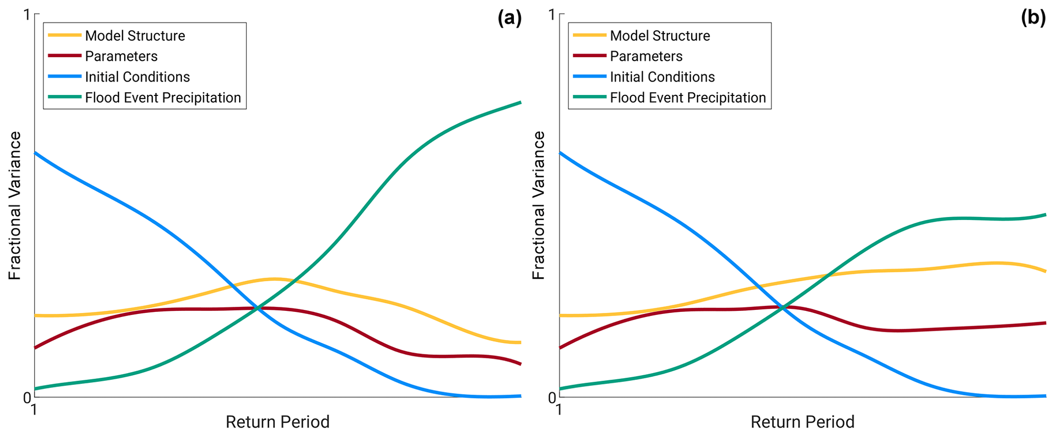
Figure 1Conceptual contribution of relative variance contribution from initial conditions (blue), model parameters (red), model structure (orange), and precipitation event forcing (green) across return periods (larger return periods towards the right) for (a) the base case and (b) one possible alternative, where model structure has similar importance to precipitation event forcing for extreme events.
The Island Park Dam (Idaho) and Altus Dam (Oklahoma) watersheds are used as representative basins of mountainous snowmelt (Island Park) and semiarid high plains (Altus) hydroclimates, respectively. These basins were selected because not only are they representative of the dominant hydroclimates of the western USA, they also have been the subject of past flood studies where basin delineations, observed streamflow, and precipitation frequency distributions were developed by Reclamation (2016a).
Island Park (Fig. 2a) is located on Henrys Fork River, approximately 56 km north of Ashton, Idaho, and water stored at Island Park is used locally for irrigation. The Island Park watershed is roughly 1297 km2 and includes steep mountain slopes along portions of the watershed boundary to nearly level slopes around Henrys Lake. Soils for the watershed range from low permeability clays in the west to permeable volcanic sand in the east. There are areas within the watershed which are heavily forested and other areas which are barren. Elevations within the drainage area range from 1921 m at the crest of the spillway to 3231 m at Sheep Point along the northern boundary of the watershed (Reclamation, 2016b). Island Park has a strong seasonal cycle of precipitation, soil moisture, and streamflow, with most of the watershed precipitation occurring as snow in October through May in the higher elevations. This results in a seasonal snowpack, maximized in late spring which then melts through the summer, which maximizes soil moisture and streamflow during late spring and early summer.
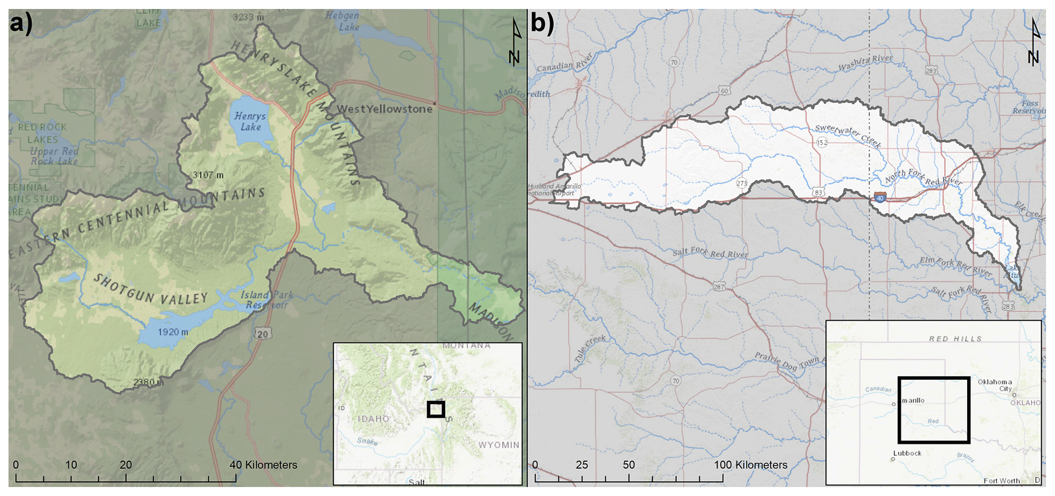
Figure 2Island Park (a) and Altus (b) watershed locations. Base layers are from © Esri (Environmental Systems Research Institute).
Altus Dam is on the North Fork Red River about 27 km north of the city of Altus, OK. The purposes of the dam and reservoir are to provide irrigation storage for lands in southwestern Oklahoma, flood control on the North Fork of the Red River, an augmented municipal water supply for the city of Altus, fish and wildlife conservation benefits, and recreation. The watershed extends from Altus Dam in Oklahoma westward to Amarillo, Texas (Fig. 2b). The watershed consists of generally rolling terrain, with medium to coarse textured soils, and spans an elevation from about 1120 m at the western edge of the basin to 450 m at the eastern outlet. This area contains many topographic features known as playa lakes (closed basins with a low area in the center that may see water storage following heavy rainfall), and thus, the total contributing area is smaller than the total area of the watershed. We used the Reclamation (2012) estimated contributing area of 5051 km2. Much of the basin above Altus Dam is devoted to agriculture, with a majority of the land cover consisting of cultivated crops, pasture, and hay production. The drainage basin contains no large forested areas, but there are treed riparian zones along the watercourses and trees in cultivated shelterbelts (Reclamation, 2012). Altus Dam is a semiarid basin that also has a seasonal cycle to precipitation, with most occurring in winter through summer, primarily as rainfall. The spring and summer rainfall events are primarily convective in nature, with sometimes very intense rainfall rates and high total accumulations over short periods of time that may coincide with peak basin soil moisture in the spring.
3.1 Modeling workflow
Our stochastic hydrologic modeling workflow includes the Framework for Understanding Structural Errors (FUSE) hydrologic modeling framework (Sect. 3.2), the shuffled complex evolution (SCE) optimization algorithm (Sect. 3.2), and precipitation frequency distributions from Reclamation (2012, 2016a) (Sect. 3.5). Additionally, we have used the law of total probability (e.g., Tijms, 2003; Nathan et al., 2003; this Sect. 3.1, the next paragraph, and Sect. 3.7) and the ANOVA method (Sect. 3.7) to compute the FF estimates and partition the variance across the workflow components, respectively. Figure 3 provides a workflow diagram describing our stochastic hydrologic modeling system.
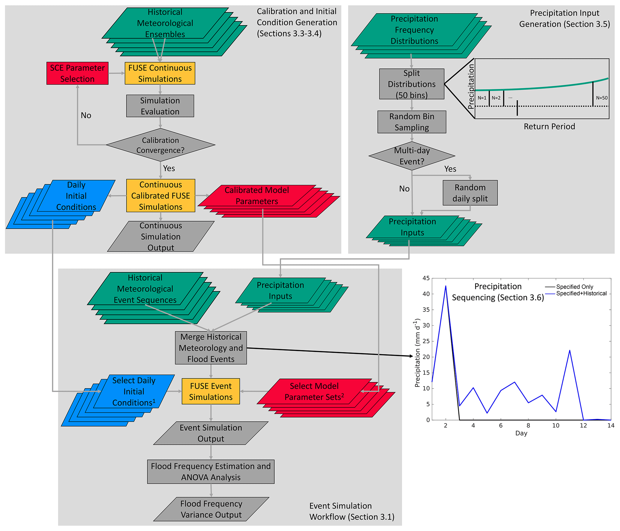
Figure 3Workflow diagram of the complete stochastic modeling system described in Sect. 3. The calibration, initial condition generation, and precipitation-input-generation steps are shown in more detail in the upper two gray panels, which then feed to the lower right gray panel. Merging of the flood event precipitation, with specified 0 precipitation days or historical meteorology, is show in the lower right figure. Color coding follows Fig. 1. 1 Select daily initial conditions are matched for a given model and parameter set and are taken as the 90th, 94th, 97th, and 99th percentile of total column moisture for that model and parameter set combination. 2 Select model parameter sets are taken as the top-performing model parameter sets from the 100 available calibrations for each model structure for each basin, following Sect. 4.1.
For each basin, hydrologic models are configured and calibrated using an ensemble of historical meteorology (Newman et al., 2015). To simplify the experimental design, we chose to represent the basins using watershed or lumped hydrologic models, removing the need to calibrate a distributed hydrologic model and add other dimensions accounting for the spatial variability of rainfall and ICs (e.g., Zhu et al., 2018). Examination of how varying spatial representation of watersheds impacts FF estimates could be the subject of further research. Long-term continuous simulations are used to generate spin-up initial conditions for event simulations (shown in the upper left panel of Fig. 3 and discussed more in Sects. 3.3–3.4). Event simulations are then performed across hydrologic models, model parameters, initial conditions, and precipitation frequency distribution estimates for two meteorology sequence possibilities, flood event precipitation only, and flood event precipitation plus historical precipitation, as discussed more in Sect. 3.6. For each precipitation frequency distribution, we split the probability density function into 50 bins, sample 25 events per bin, and perform 2500 model simulations for each possible model parameter–IC–precipitation frequency combination. This study follows the methodology used by Reclamation (e.g., Reclamation 2012, 2016b) in the stochastic flood modeling, as shown in the upper right panel of Fig. 3, and provides for uniform sampling across the precipitation frequency distribution, including extremely rare precipitation events. These precipitation inputs are then used in the event simulations with the precipitation frequency distributions representing 1 d events for Altus and 2 d events for Island Park Dam, and Island Park Dam precipitation inputs are randomly split across 2 d. Note that performing long integration continuous simulations using a stochastic rainfall simulator is another valid approach (e.g., Calver et al., 1999; Yu et al., 2019) that could be used within our general ANOVA framework, where direct specification of ICs and precipitation frequency curves would be replaced by specification of a stochastic rainfall (and other meteorological variables) generator (Yu et al., 2019). Finally, flood events are defined as 14 d volume floods for Island Park and single day peak flows at Altus.
We implemented a factorial experimental design, using all combinations of the 10 hydrologic models (Sect. 3.2), 11 parameter sets (10 for Altus Dam) (Sect. 4.1), four initial condition sets (Sect. 3.4), and 11 precipitation frequency estimates for Island Park Dam (three precipitation frequency estimates for Altus Dam; Sect. 3.5) for a total of 4840 combinations, with 2500 model simulations per combination, resulting in 12.1 million event simulations for Island Park Dam (hereafter referred to as Island Park) and 3.3 million event simulations for Altus Dam (hereafter referred to as Altus). The different precipitation frequency estimates come from the fact that this project leveraged previously completed studies for these data. We do not believe that this will significantly impact the results, as the ANOVA analysis takes these sampling differences into account.
3.2 Hydrologic model framework
The FUSE hydrologic modeling system is a freely available, modular modeling framework that enables the developing and testing of many conceptual hydrologic models in a single computational framework. It incorporates multiple parameterizations for many hydrologic fluxes (or processes) at the individual flux level, with each equation formulated as a function of the model state, each in a separate code module. This allows the numerical solver to be separated from the flux parameterizations so that every FUSE configuration relies on exactly the same numerical scheme. FUSE also incorporates a conceptual temperature index snow model, using elevation bands with user-specified precipitation and temperature lapse rates to represent seasonal snowpack and changes in meteorology with elevation. Control at the individual flux level is key to understanding how changes in process representation affect the modeling system behavior. Clark et al. (2008) and Henn et al. (2015) provide more details on the FUSE modeling framework.
FUSE uses several configuration files in which the user can specify the model decisions for process representation, numerical solver parameters, model calibration options, access to input and output data, etc. The structural modularity in FUSE is underpinned by one file prescribing the equations to be used for each model component. This file can be changed independently from the other model settings, enabling the user to isolate the effects of the model structure decisions on the simulations. FUSE has been coupled with the SCE optimization algorithm (Duan et al., 1993) to calibrate any hydrologic structure the user specifies. SCE is a robust global optimization algorithm that is widely used across the operational and research communities. FUSE uses the network common data format (netCDF) for all input and output data streams (forcing meteorology, any available observations for calibration, calibration results, and simulated states and fluxes), using the same file format regardless of hydrologic model configuration. Overall, the design of the FUSE system enables easy configuration, calibration, and simulation of multiple hydrologic models for long term continuous simulations or short event simulations.
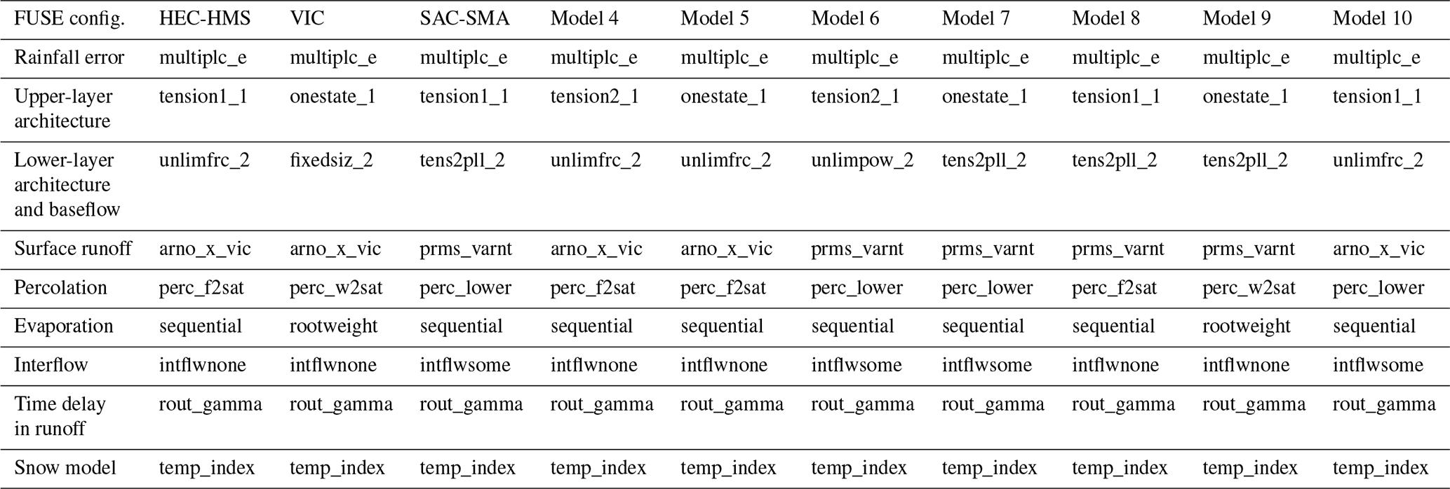
FUSE is first used to mimic three widely used hydrologic models, namely the Hydrologic Engineering Center–Hydrologic Modelling System (HEC-HMS) model (Bennett, 1998), the variable infiltration capacity (VIC) model (Liang et al., 1994), and the SACramento–Soil Moisture Accounting (SAC-SMA) model (e.g., Anderson, 2002). This provides a relatable base set of models to operational groups within the USA. Note that the FUSE instantiations of the models only mimic the actual models cited. FUSE does not use the same numerical solver, some process simplifications are made (particularly for VIC, where we simplify evapotranspiration), different parameter estimations schemes are used, and FUSE does not contain the same coding errors as the original models (see Clark et al., 2008, for FUSE details). As a result, when mimicking a pre-existing model using a modular framework, some substantial differences between their simulations can exist (Knoben et al., 2019). We then assembled seven other hydrologic model structures by varying particular processes from the three base models for a total of 10 structures that we used to compute FF estimates for both basins (see Table 1 for the full list). Again, we use a watershed or lumped spatial configuration of FUSE in this study.
3.3 FUSE meteorological forcing and calibration
All 10 hydrologic models for both basins were calibrated using the SCE optimization algorithm (Fig. 3). We used the Kling–Gupta efficiency (KGE) and the root mean squared error (RMSE) as objective functions because the choice of objective function is subjective and dependent on available data and user needs. Additionally, recent work has highlighted that careful consideration needs to be given to the choice of objective function for high-flow events (Mizukami et al., 2019). Root mean squared error (RMSE) is directly related to the Nash–Sutcliffe efficiency (NSE). Furthermore, it can be shown that RMSE/NSE is made up of the following three component contributions to the total value (Murphy, 1988; Clark et al., 2021): correlation (r), variability (α), and bias (β). The Kling–Gupta efficiency (KGE) is a reformulation of these same components, which allows the user to easily understand their individual contributions to the total KGE value (Gupta et al., 2009) and is shown in (Eq. 1) as follows:
where EDs is the scaled Euclidian distance from the ideal point, and sr, sα, and sβ are scale factors to adjust the weighting of the correlation, variability, and bias terms (each scale factor is typically set to 1). The KGE is also beneficial to use because the scale factors can be adjusted to emphasize the different components of KGE. Here we tested RMSE and KGE calibrations using daily streamflow and KGE computed using annual peak flow values. We also examined modifying the KGE sα scale factor from 1 to 5 to emphasize model flow variance in an effort to better capture flood peaks. Inflated sα values resulted in model behavior very similar to KGE using annual peak flows, in agreement with Mizukami et al. (2019), and are not discussed further.
Table 1FUSE hydrologic processes (far left column) and the various selected process representations for the 10 hydrologic models.
A maximum of 40 000 model runs was allowed for the SCE calibration of each model structure and basin. Reconstructed daily inflow data from Reclamation (2016b) was used for Island Park, while annual peak flow data developed by Reclamation (2012) was used for Altus due to lack of better available data for calibration at the time of this study. The impact of these different objective functions and calibration data for the basins will be discussed in Sect. 4.
The meteorological forcing data consisted of a 100-member ensemble of gridded precipitation and temperature at 6 km resolution, as described in Newman et al. (2015). Observations of precipitation and temperature and the process of projecting point measurements to grids across sometimes complex terrain are inherently uncertain. This ensemble data set was designed to estimate those uncertainties and provide many plausible historical traces for hydrologic model applications. The ensemble precipitation and temperature grids are merged to the watershed scale using fractional areal weighting for all meteorological grid cells that intersect a basin polygon. Watershed-scale forcing derived from each individual meteorological ensemble member was used to calibrate each hydrologic model, resulting in a 100-member ensemble of calibrated model parameters for each model for each basin (100 ensembles × 10 models × 2 basins; Fig. 3). Because of the available observational data, different spin-up and calibration periods were used. For Island Park, the hydrologic models were spun up for water years (WYs) 1970–1979 and calibrated on WY 1980–2014 (35 WYs), while Altus was spun up for WY 1980–1984 and calibrated on WY 1985–2011 (27 WYs). Again, while the number of WYs for both catchments is similar, data availability meant that Altus calibration only relied on annual peaks, while for Island Park daily streamflow values were used. Finally, given the limited data for both basins, we chose not to withhold any data for out-of-sample performance assessments because this study is not focused on out-of-sample model performance, and we preferred to have the largest possible calibration sample size.
3.4 Initial condition specification
Continuous simulations were performed using the optimized model parameters and full model states were output each day for the full calibration periods for each hydrologic model and basin. These states were sampled to determine the ICs for the event simulations. Sampling initial states from continuous simulations has the advantage of providing ICs that are consistent with the specific hydrologic model and parameter set versus applying random IC perturbations. Applying random perturbations to an IC may result in unrealistic states and subsequent simulation results.
For Island Park, the focus was on ICs from April through June that had minimal (<10 mm) snow water equivalent snowpack to represent flood events near the end of the snowmelt season around peak climatological soil moisture storage. For Altus, the focus was on late winter through midsummer ICs (February–July), when both soil moisture and precipitation event intensity and volumes are near their climatological maximums. For both basins and all models, four ICs were sampled in the top 10 %, i.e., the 90th, 94th, 97th, and 99th percentiles of total column soil moisture within all validation years and selected months. Here we chose to focus on wetter ICs, following the general Reclamation FF estimation methodologies (e.g., Reclamation 2012, 2016b, 2018). However, we show results across even frequent return periods, and the reliance on only wet ICs may influence the importance of IC uncertainty for these more frequent return periods (Yu et al., 2019). The assumption that larger floods are associated with wetter ICs may not be valid in all hydrologic regimes, especially in more arid environments where conditions, such as surface sealing and rock-mantled slopes, may actually result in more severe flooding under intense short-duration thunderstorms. While the basins tested here did not consider those conditions, a wider distribution of ICs could be considered in future work which, again, may increase the importance of ICs in flood response.
3.5 Precipitation frequency estimates
Regional frequency analysis (RFA) is a useful method for extending the period of record in environmental data sets by means of a space-for-time substitution, where additional information in space supplements the lack of information in time. The basic assumption of RFA is that extreme events recorded at stations located within a predetermined homogeneous region can be described by the same probability distribution. By scaling the data by the respective at-site mean (ASM), the user assumes that a single probability distribution is valid for every location within the homogeneous region, while the magnitude can vary spatially.
The L-moments method (Hosking and Wallis, 1997) is one example of a regional frequency method. The basis of the L-moments algorithm is that linear combinations of moments can be used to estimate model parameters for extreme value distributions. The moments of interest (also referred to as L-statistics) include L-CV, L-skewness, and L-kurtosis and are computed for every site utilized in an analysis. Regional moments are developed using weighted averages of the site-specific moments, where the weight is proportional to period of record. The regional L-moments are then used to define the regional growth curve (RGC), a dimensionless quantile function that represents the cumulative distribution function of the frequency distribution valid for all sites located within the homogenous region. Site-specific precipitation–frequency estimates (Qi(F); Eq. 2) are developed by scaling the RGC (q(F)) by a site-specific ASM (μi), allowing the magnitudes of precipitation–frequency estimates to vary spatially across the region of interest.
Reclamation (2016a) developed median and uncertainty precipitation–frequency curves for the Island Park watershed using a regional L-moments approach combined with Latin hypercube resampling procedures. More specifically, the authors used annual maximum 2 d precipitation totals from 45 stations in a homogeneous region surrounding the Island Park watershed to estimate parameters of the four-parameter Kappa distribution. The authors used Latin hypercube sampling methods in R, via the qnorm function, to perform Monte Carlo sampling to create 300 parameter sets using variations in five parameters, namely the at-site mean, regional L-CV, regional L-skew, regional L-kurtosis, and areal reduction factor (ARF), to account for converting point precipitation frequency estimates to the basin-average precipitation frequency estimates. For Island Park, the authors of that study applied a constant ARF for all exceedance probabilities, even though ARFs have been shown to vary by exceedance probability (e.g., Bell, 1976). More specifically, Reclamation (2016a) multiplied the point-specific precipitation–frequency curve by a constant ARF of 0.85, which they estimated using a historical point and basin-average precipitation depths available in HMR 55A (Hansen et al., 1988) and HMR 57 (Hansen et al., 1994). Results from the Island Park analysis include 11 frequency distributions (5th, 14th, 23th, 32th, 41th, 50th, 59th, 68th, 77th, 85th, and 95th percentiles). Kappa parameters from Reclamation (2016a) are reproduced in Table 2. During the stochastic simulations performed here, we force 2 d historical precipitation inputs to equal the basin-average magnitudes sampled from the 2 d precipitation frequency curve valid over the Island Park watershed.
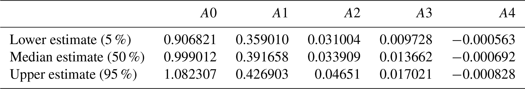
Similarly, Reclamation (2012) developed precipitation–frequency estimates, including median and uncertainty bounds for the Altus watershed, using a regional L-moments approach combined with Latin hypercube sampling procedures. The authors focused on annual maximum 1 d (or 24 h) precipitation totals recorded at 482 stations, with at least 5 years of data, and used Latin hypercube sampling to produce 150 parameter sets based on variations in the following same five parameters listed above: at-site mean, regional L-CV, regional L-skewness, regional L-kurtosis, and ARF. The ARF for Altus was developed using a linear relationship between point and basin-average storm totals, using 12 different storms that impacted the Altus watershed identified in HMR 51 (Schreiner and Riedel, 1978), HMR 52 (Hansen et al., 1982), and HMR 55A (Hansen et al., 1988). The Altus report provides all precipitation–frequency estimates in the form of fourth-order polynomials, with coefficients reproduced in Table 3. Similar to Island Park simulations, we force 1 d historical precipitation events to equal basin-average magnitudes sampled from the 1 d precipitation frequency curve valid over the Altus watershed. Median precipitation frequency curves for both basins, including the 5th and 95th statistical sampling percentiles, are shown in Fig. 4.
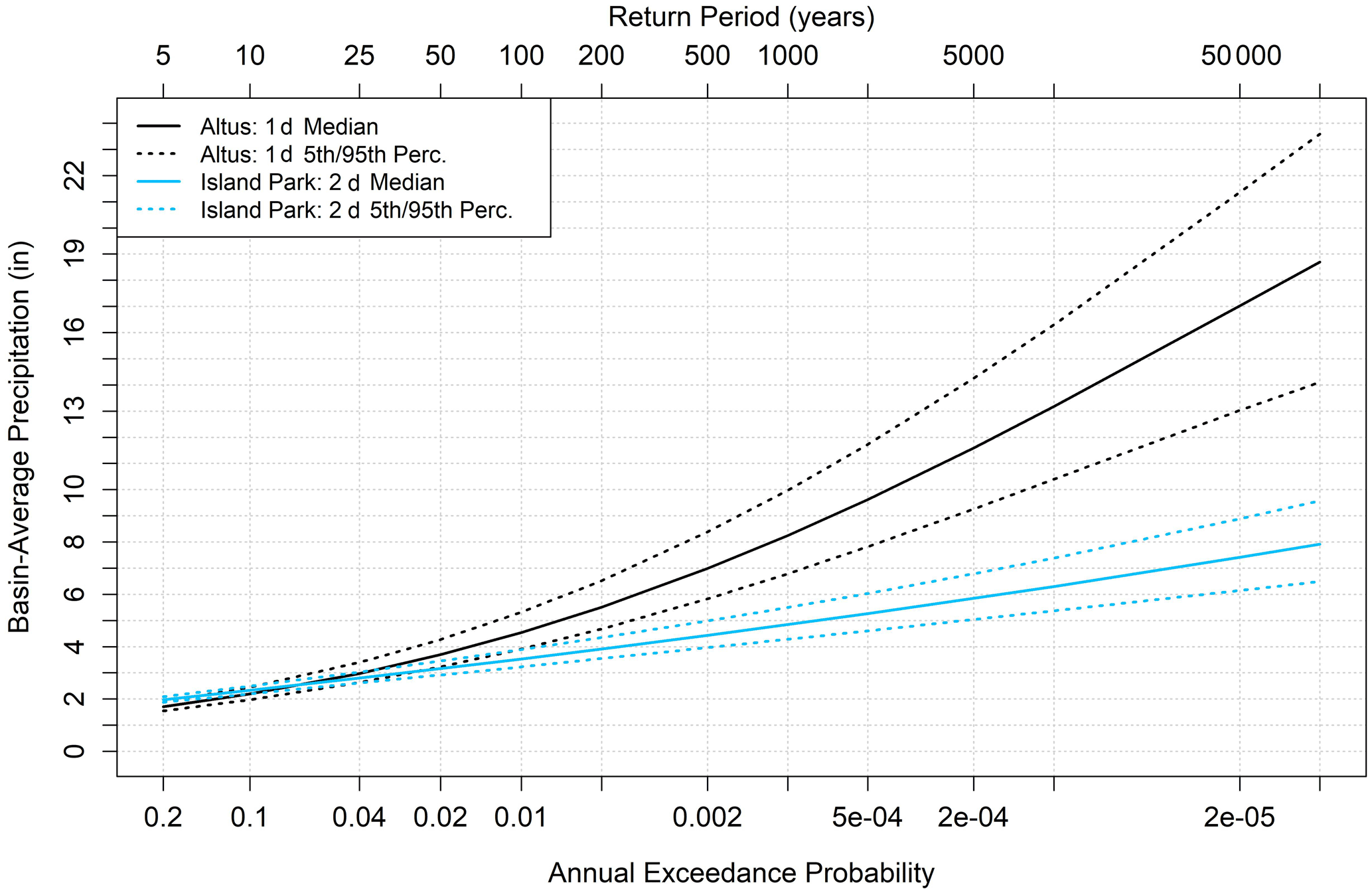
Figure 4Precipitation frequency estimates for Altus (1 d; blue) and Island Park (2 d; black) including the median (solid), and the 5th and the 9th percentiles (dashed).
Table 2Parameters used to define the four-parameter Kappa distribution. Table is reproduced from Table 4.5 in Reclamation (2016a).
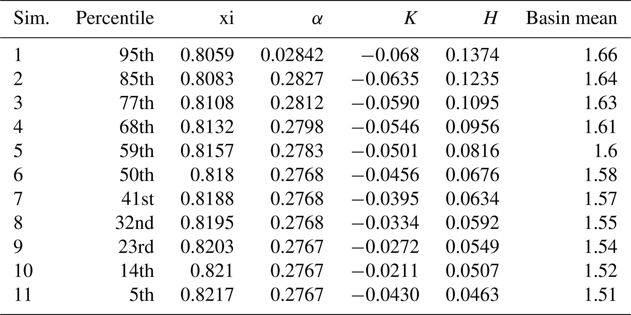
Table 3Polynomial coefficients (fourth order) that describe the lower, median, and upper precipitation frequency curves for Altus. Table reproduced from Table 5.7 in Reclamation (2012).
3.6 Meteorology specification
Some stochastic modeling studies at Reclamation force the rainfall–runoff model with a specified precipitation input (e.g., 2 d input from a precipitation frequency distribution), followed by no precipitation for the remaining simulation time (Reclamation, 2018). The lack of additional precipitation after the specified precipitation input is not based on any physical reasoning; thus, we examine both zero and historical precipitation sequences after the specified precipitation input (2 d at Island Park and 1 d at Altus; Sects. 2 and 3.5). In the specified meteorological sequence, we set precipitation to zero after the specified precipitation input. In the historical meteorology sequence, we randomly sample ensemble member meteorology using the same event start date from the selected IC. In both meteorological sequences, the specified precipitation forcing is exactly the same. Future work should examine event sequencing in greater detail, particularly to quantify the impacts of possible future circulation changes on FF estimates and sensitivities.
3.7 Flood frequency estimation and ANOVA
As noted in Sect. 3.1, the total probability theorem is used to compute modeled basin runoff at return periods of 2, 5, 10, 20, 50 100, 500, 1000, 5000, 10 000, 50 000, and 100 000 years from the stochastic simulations for all model, parameter, IC, and precipitation distribution combinations for both meteorology sequences. To do this, the distribution of flood event runoff was divided into 50 bins, following the division of the precipitation frequency distributions (Fig. 3; upper right box). All event simulations exceeding the modeled runoff threshold in a given bin were counted, and then the probability of exceedance of that runoff threshold was computed as the summation of the probability of precipitation inputs occurring in that specific bin times the number of flood events. We then used linear interpolation to estimate the runoff at the specific return periods listed above. Again, 14 d volumes are used at Island Park and maximum daily runoff are used at Altus to define the flood event.
An ANOVA analysis is then performed on the runoff values for all the return periods for both meteorology sequences and basins. The ANOVA framework is a computationally frugal way to estimate individual component contributions to the total variance of a variable such as runoff by relying on a sum of squares decomposition. ANOVA analyses have been widely used in hydrometeorology to separate the components of future climate changes (Hawkins and Sutton, 2009; Lehner et al., 2020) and to determine which elements of the model chain contribute most to the spread of the projected changes in streamflow (Bosshard et al., 2013; Addor et al., 2014; Breuer et al., 2017; Chegwidden et al., 2019). By estimating the fractional (relative) variance contributions of each factor and all (two) factor interactions, we identified the pieces of the modeling workflow which contribute most to FF sensitivity for each return period. We used the anovan MATLAB function, as implemented in MATLAB version 9.8.0.1380330 (2020a) update 2. This function allows for N-way ANOVA computations with mixed continuous and categorical predictors and specification of the interaction terms to be estimated (https://www.mathworks.com/help/stats/anovan.html, last access: 2 March 2021). Here we specify model structure and parameters as categorial predictors and precipitation event forcing and initial conditions as continuous predictors. Precipitation event forcing and initial condition values are normalized before the ANOVA analysis was performed. Finally, we perform a subsampling and bootstrapping of the effects that have more samples than the effect with the fewest samples (e.g., for Island Park, ICs have four samples and precipitation frequency distributions have 11 samples), following Bosshard et al. (2013). Disparate sample sizes can bias the fractional variance estimates, overestimating the contributed variance for effects with more samples. Performing subsampling with bootstrapping (n=1000) alleviates the bias (Bosshard et al., 2013).
When examining daily flow time series, the KGE and RMSE based on daily flow produce more realistic simulations than the KGE using annual peak flow, as seen in Fig. 5. This is a somewhat expected result as the interval metric contains no time information (correlation) on the daily scale. The daily KGE-based calibration outperforms the daily RMSE-based calibration, where the daily RMSE-based calibration underestimates the flow variance (not shown), in agreement with past studies (Gupta et al., 2009). The annual peak-flow-based KGE calibration represents the peak flows well (with some overestimation) but has large differences in event recession curves, with overestimation of flow in the days and weeks immediately following high-flow events. This erroneous recession curve representation would result in very different volume-based floods versus daily metric-based calibrations.
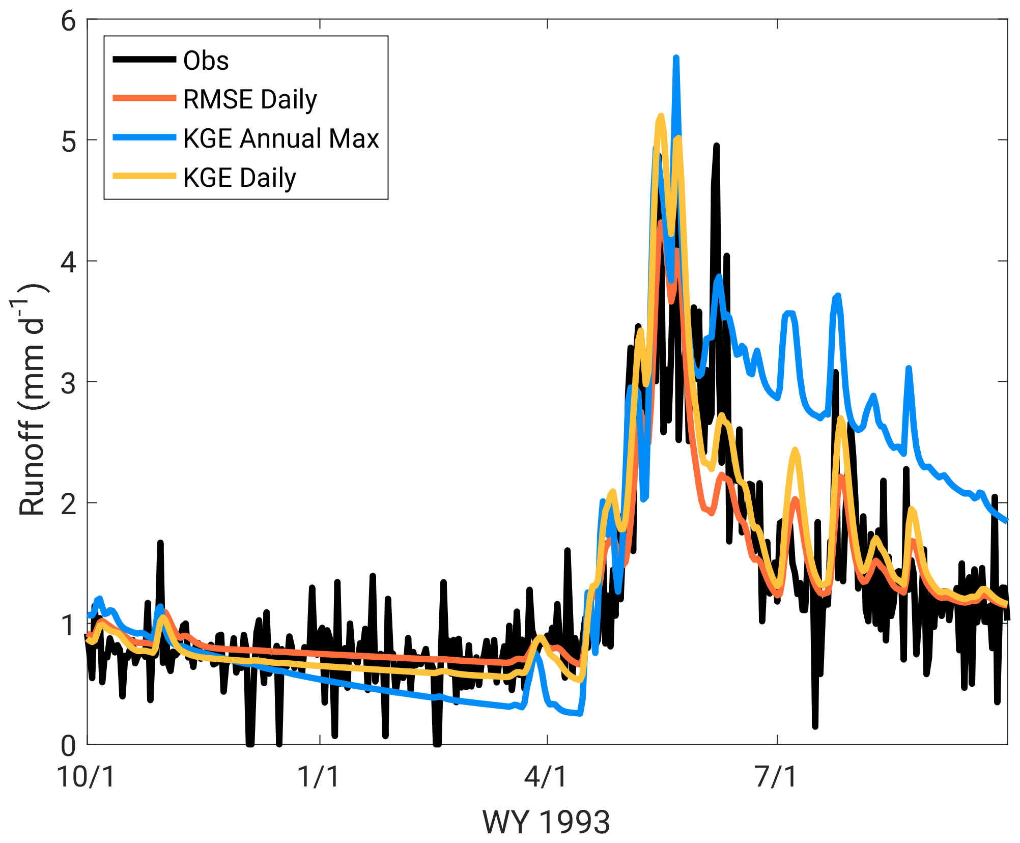
Figure 5Island Park calibration period runoff for water year (WY) 1993, with RMSE using daily flow, KGE using daily flow, and KGE using annual maximum flow.
Given the above calibration characteristics and the available calibration data at Island Park (daily flow) and Altus (annual peak flow), daily KGE was selected as the calibration metric for Island Park and annual peak-flow-based KGE as the calibration metric for Altus (Sect. 3.3 defines these calibration metrics). Daily KGE provides the best all-around simulation when considering daily peak flows and volume integrations over days to weeks at Island Park. For Altus, calibrating to yearly peak-flow-based KGE provided a better overall peak flow calibration than RMSE calculated using annual peak flows, likely due to the reformulated weighting of bias and variance as compared to RMSE. Again, these results agree with Mizukami et al. (2019), who examined some of the same calibration metrics using multiple hydrologic models and hundreds of basins across the contiguous USA. They found that KGE outperforms RMSE-based (or NSE-based) calibrations, and that peak flow metrics do outperform KGE for peak flow simulation but result in a much degraded daily model performance with sometimes severe modeled flow biases.
Figure 6 highlights the final cumulative density function (CDF) of the calibrated KGE for all 10 models for Island Park (Fig. 6a) and Altus (Fig. 6b). It is not possible to make direct performance comparisons between the models at the two basins, given that the KGE values are based on daily (Island Park) and annual peak runoff (Altus). However, in a broad sense, model behavior at Island Park is much more constrained than Altus, based on the relative ranges of calibration scores for each basin (different x-axis ranges from left to right panels). These differences informed the model parameter sampling strategies and show that the model behavior at Island Park is more constrained than at Altus along the model parameter dimension.
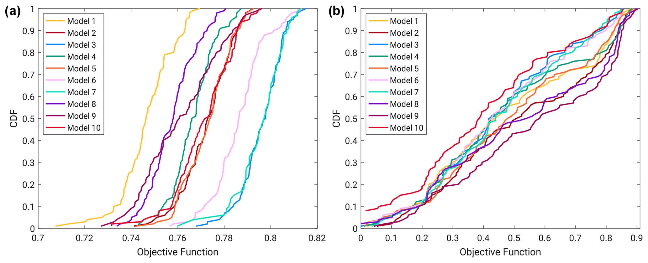
Figure 6(a) Island Park daily flow calibrated KGE distributions for all 10 models. (b) Altus yearly peak flow calibrated KGE distribution for all 10 models.
4.1 FUSE parameter set selection
The 100 parameter sets available for each model and basin were subsampled for the final FF event simulations. Because Island Park had more available data for calibration (Sect. 3.3), the final calibrated model performance was very similar across the 100 members for all 10 hydrologic models. Therefore, 11 parameter sets spanning the full range of model performance were sampled for each hydrologic model using the 1st, 10th, 20th, 30th, 40th, 50th, 60th, 70th 80th, 90th, and 99th percentiles of the cumulative density function (CDF) of the calibration objective function. For Altus, the calibrated model behavior was less constrained due to the much smaller amount of calibration data available. Therefore, the 10 best-calibrated parameter sets for each hydrologic model were used, which constrained model-parameter-induced differences in model behavior but still not to the same level as Island Park.
The ANOVA analysis was performed using the full complement of FF estimates for both basins (Sect. 3.7) and both meteorological sequences (Sect. 3.6). All fractional variance contributions are normalized by the total variance in the FF estimate for each return period such that if a component has a fractional variance of 0.5 then that component contributes half of the total variance for that return period. The plots represent the 2, 5, 10, 50, 100, 1000, 10 000, 50 000, and 100 000 year return periods. For Figs. 8–13, the specified input meteorological sequence is always in panel (a) and the historical input meteorology sequence is always in panel (b), and the color coding follows Fig. 1. Interaction terms are a blend of the two primary components (e.g., model structure–model parameter interactions are red–orange).
First, normalized FF plots, including all possible effect combinations for both models, are shown in Fig. 7. Annual exceedances at Island Park in the mean follow a nearly linear trend on the semi-log x-axis plot, with the range of possible values having relatively higher spread at larger return intervals (Fig. 7a), which is consistent with the hydrology of Island Park being a less flashy, more snowmelt-flow-dominated basin. The normalized FF curve at Altus is highly nonlinear, even with a semi-log x axis, with little flow for many small return periods (Fig. 7b). Sharp increases in flood responses after roughly the 500 year return period are seen, with the normalized spread larger than at Island Park for the largest return periods (50–100 000 years). The normalized FF plots in Fig. 7 have similar shapes to the precipitation frequency distributions (Fig. 4) for both basins, where Island Park has a more gradual increase as compared to Altus, which has much larger rare precipitation inputs.
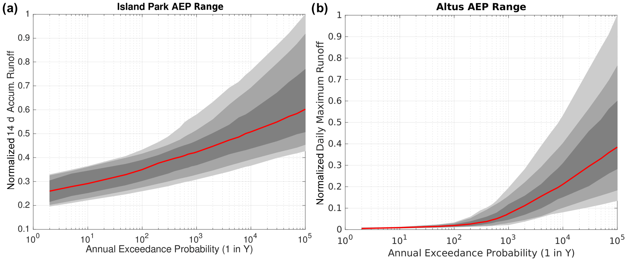
Figure 7Normalized (by maximum possible flood runoff) FF curves, with the median in red, and the interquartile range (25th–75th percentiles), in dark gray, the 10th–90th percentile spread, in medium gray, and the minimum to maximum spread, in light gray, for (a) Island Park and (b) Altus.
5.1 Island Park
ANOVA results using all available model structures, sampled parameter sets, sampled ICs, and sampled precipitation frequency distributions for Island Park are shown in Fig. 8. When all model structures are included, ICs dominate the frequent floods less than about 5000 years, while the precipitation frequency distribution is the most important for rarer floods. This agrees with other recent studies examining IC contribution to FF estimates using ANOVA or similar frameworks (Peleg et al., 2017; Zhu et al., 2018). Model structure consistently contributes roughly 20 % of the variance and is generally the second most important effect across all return periods outside of 1000–10 000 year flood, where ICs, precipitation frequency curves, and model structure vary in leading, secondary, or tertiary importance, depending on the meteorological sequencing. Model parameters and interaction terms contribute roughly 10 % of the variance for less frequent floods for both meteorological sequences. For rare floods with return periods larger than 50 000 years, precipitation input is about twice as important as model structure and 3 times more important than ICs for the specified meteorological sequence, while, for historical meteorological sequencing (Sect. 3.6), the precipitation input is only about 1.5 × more important than model structure for 100 000 year floods.
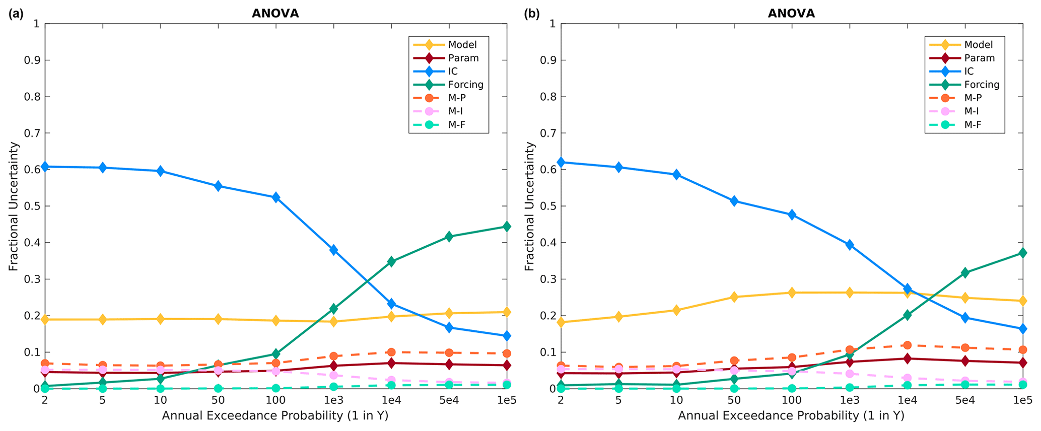
Figure 8Island Park fractional variance contributions using all 10 model structures for the (a) specified meteorological sequence and (b) historical meteorological sequence. Only interaction terms that contribute significant variance are shown in Figs. 6–11.
Figure 9 presents the fractional variance contributions for Island Park using the following three base models: HEC-HMS, VIC, and SAC-SMA (Sect. 3.2; Table 1). Similar to all models, ICs and the precipitation frequency distribution specification are the most important for frequent and extreme floods, respectively. Model structure is the second most important contributor to frequent floods, but for return periods larger than 1000 years, model structure–parameter interactions become as or more important than the model. Again, moving from the specified to historical meteorological sequence decreases the variance contribution of precipitation frequency distributions and increases the importance of model structure, model structure–parameter interactions, and ICs across all return periods (compare Fig. 9a to b). This is somewhat counterintuitive but may be related to the fact that soil states can strongly influence recession curve characteristics, and the additional precipitation in the historical meteorological sequence (from zero after the specified input in the specified sequence) is either stored or released within the 14 d volume flood integration period depending on model structure, parameters, or ICs.
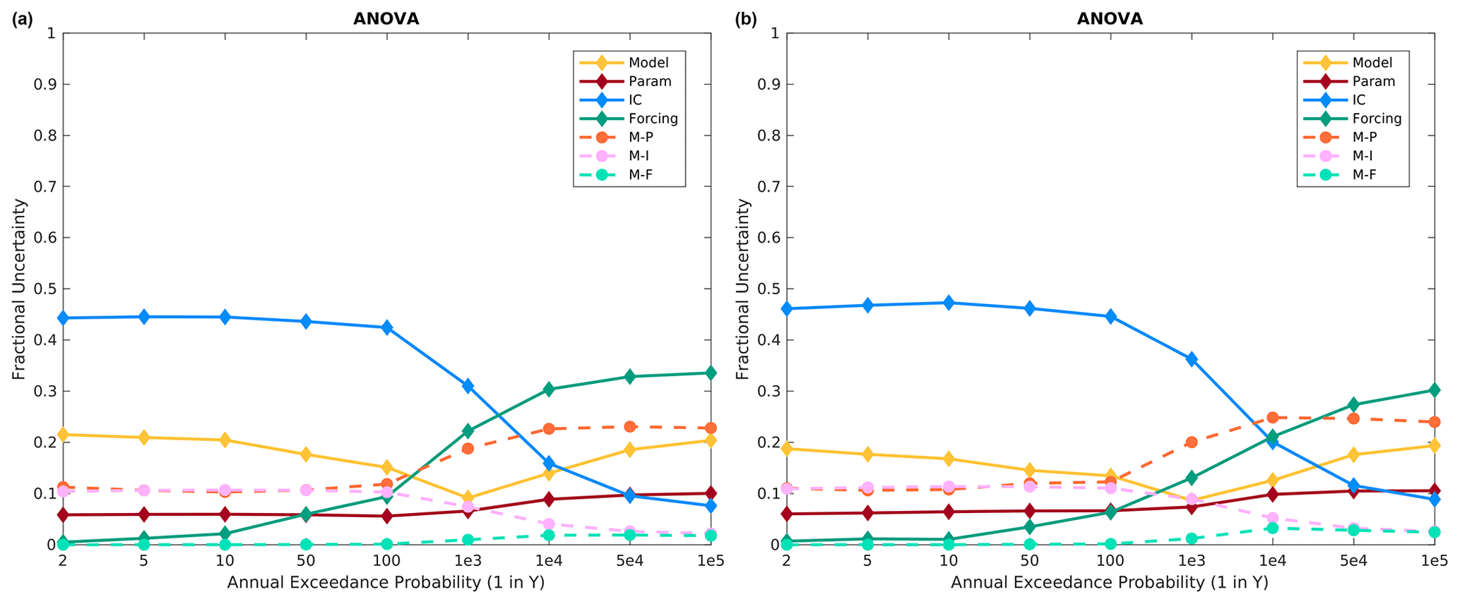
Figure 9Island Park fractional variance contributions using the three base models, namely HEC-HMS (model 1), VIC (model 2), and SAC-SMA (model 3), for the (a) specified meteorological sequence and (b) historical meteorological sequence.
Using a different combination of the 10 possible model structures results in a slightly different conclusion. The set of simulations presented in Fig. 10 represents the set of three hydrologic models that generates the largest flood responses to larger precipitation event forcing. Overall, the precipitation frequency distribution specification is still the most important for extreme floods, and ICs are most important for very frequent floods, but model structure contributes a larger fraction of the total variance across all return periods and is often of similar magnitude to either ICs or precipitation frequency distribution changes (Fig. 10). Here we see that moving from the specified to historical meteorological sequence increases the importance of model structure (compare Fig. 10a to b). This is because these three model structures (Table 1) have more variation between each other, given additional precipitation input, than the variability in runoff changes due to ICs. Differences in surface runoff versus subsurface storage and slower baseflow appear to be driving the model structure variability and are discussed more in Sect. 6.
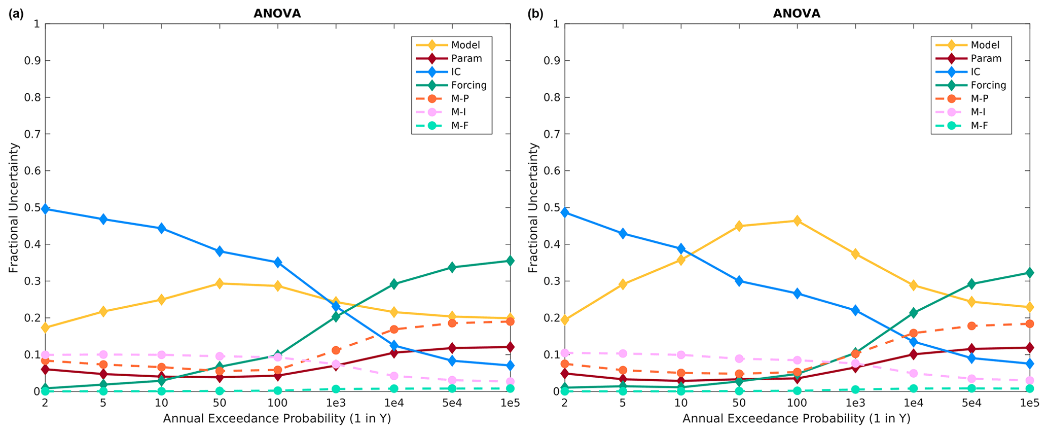
Figure 10Island Park fractional variance contributions for the three most responsive model structures (i.e., structures associated with the largest runoff/precipitation ratio), namely HEC-HMS (model 1), HEC variant (model 4), and a SAC-SMA/HEC-HMS combination (model 6), for the (a) specified meteorological sequence and (b) historical meteorological sequence.
5.2 Altus
The ANOVA results, using all available model structures, sampled parameter sets, sampled ICs, and sampled event forcings, for Altus are shown in Fig. 11. Similar to Island Park, ICs are most important for frequent floods, while precipitation event forcing is most important for rarer floods. There are two differences of note here. First, precipitation frequency distributions are generally more important across return periods at Altus versus Island Park. Second, while model structure is slightly less important, model parameters and model structure–parameter interactions are of similar importance to model structure, such that the combination of model structure and parameter effects and interactions is as important as precipitation frequency distributions across both meteorological sequences (Sect. 3.6). Finally, it is evident that meteorological sequencing is inconsequential at Altus, which makes intuitive sense given the single day peak flow metric for Altus versus the 14 d integrated volume metric at Island Park (Sects. 3.1 and 3.7).
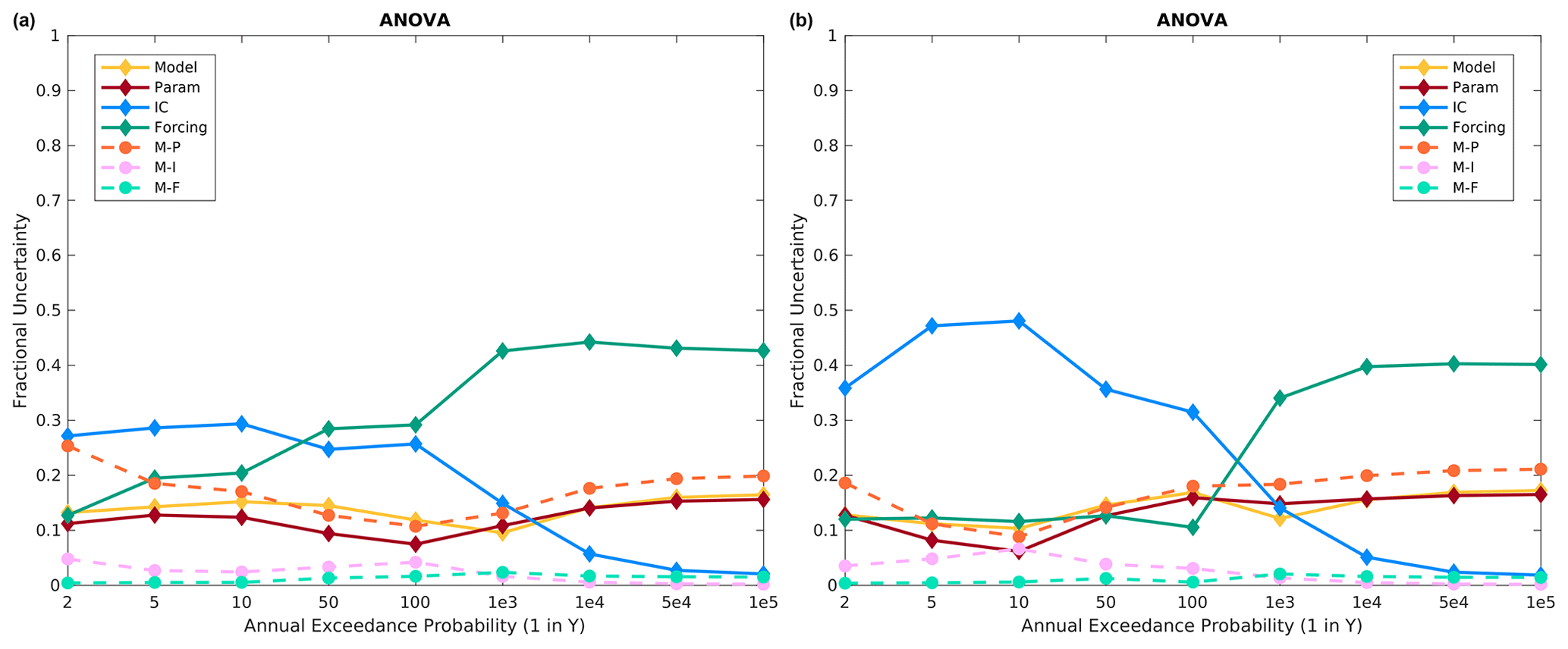
Figure 11Altus fractional variance contributions using all 10 model structures for the (a) specified meteorological sequence and (b) historical meteorological sequence.
The ANOVA results for Altus, using the three base models, show a similar picture as for Island Park. ICs almost always contribute the most variance for frequent floods (less than a few hundred years), and the precipitation frequency distributions are the most important for larger floods (Fig. 12). However, the precipitation frequency distributions are even more important for Altus than at Island Park, particularly for the historical meteorological sequence, as they contribute around 50 % of the total variance for 50 000–100 000 year floods as compared to around 30 % at Island Park. Model structure and model structure–model parameter interactions are of secondary importance across essentially all return periods. Again, moving from specified to historical meteorological sequencing does not change the picture significantly at Altus (compare Fig. 12a to b), which is expected, as the flood metric is the single day maximum flow and generally single day maximum flow is directly related to the extreme precipitation event input and not subsequent smaller precipitation inputs.
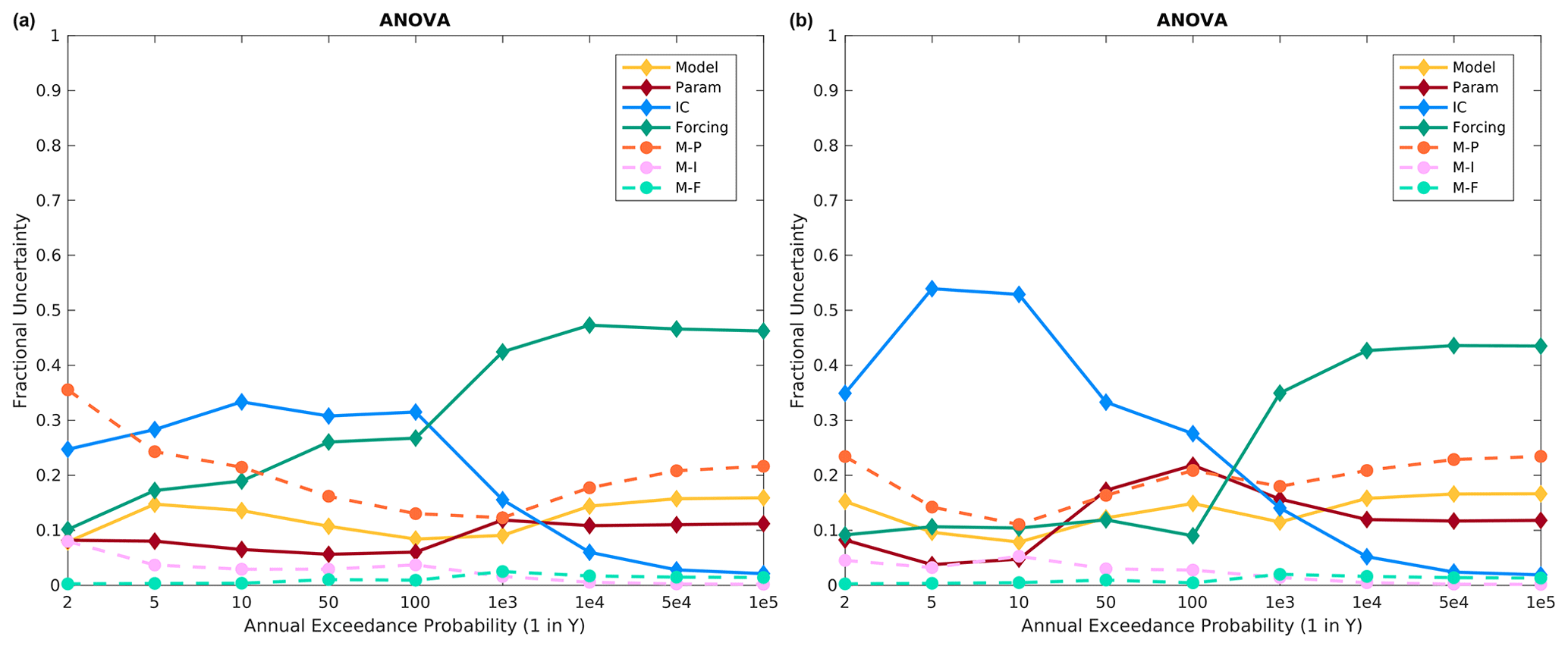
Figure 12Altus fractional variance contributions using the three base models, namely HEC-HMS, VIC, and SAC-SMA, for the (a) specified meteorological sequence and (b) historical meteorological sequence.
Further examination of multiple model combinations at Altus revealed that using the two most disparate model responses, i.e., SAC-SMA (model 3) and the SAC-SMA/HEC-HMS combination (model 6) models, results in a substantial increase in the importance of model parameters and model structure–model parameter interactions (Fig. 13). In fact, model structure–model parameter interactions contribute the most variance across all return periods in this case. Additionally, model structure and model parameter effects contribute similar variance to the precipitation frequency distributions. Again, moving from specified to historical meteorological sequencing does not substantially change the message here as expected (compare Fig. 13a to b). For this case, the model responses are starkly different, such that it may be possible to rule out one of the model structures as plausible; however, model structure selection work is outside the scope of this study.
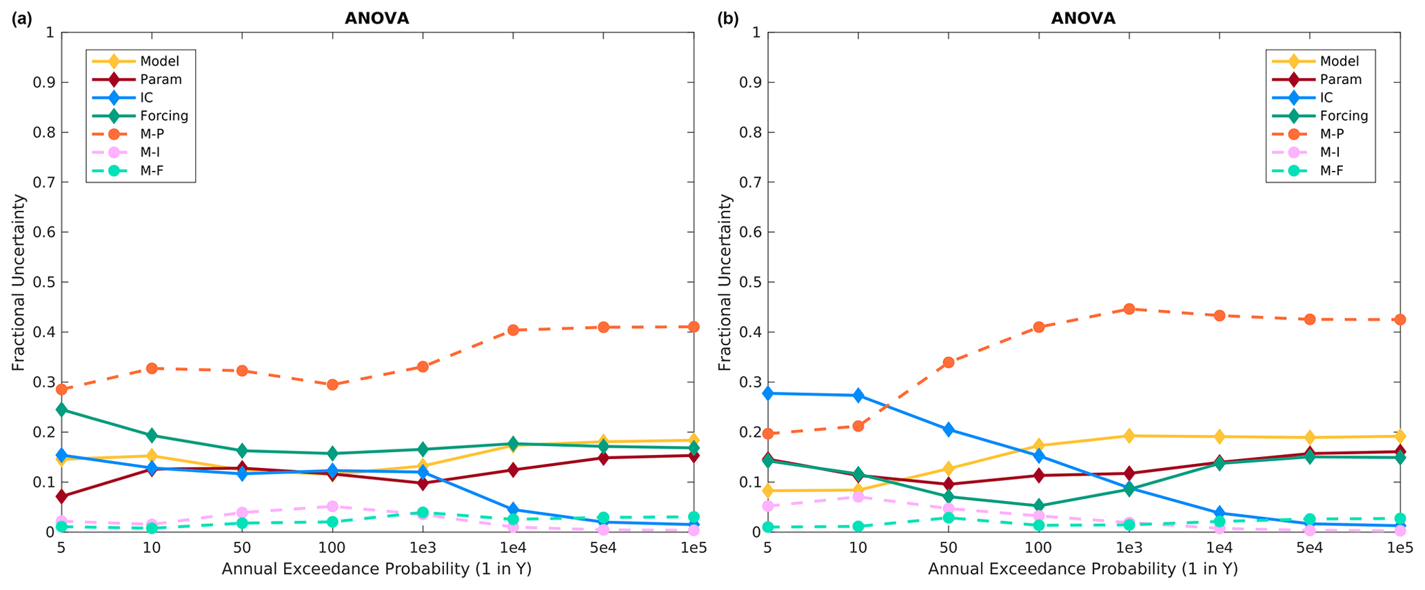
Figure 13Altus fractional variance contributions for the two most disparate flood responses, namely SAC-SMA (model 3) and a SAC-SMA/HEC-HMS combination (model 6), for the (a) specified meteorological sequence and (b) historical meteorological sequence.
The results of this study demonstrate that workflow and methodological decisions impact hydrologic model behavior and the final variance estimates of an FF study. This suggests that careful consideration of the various components of stochastic flood modeling should be undertaken. To our knowledge, the inclusion of model structure into FF estimate sensitivity analysis is a novel contribution to our understanding of stochastic flood modeling systems. We reaffirm that calibration metrics only constrain model behavior for components of the hydrograph most related to the calibration metric (e.g., Mendoza et al., 2015; Mizukami et al., 2019). For streamflow-based calibration, KGE is a metric that provides balanced model behavior across all components of the hydrograph because of its formulation and should be used over RMSE/NSE if possible. Furthermore, calibration metrics focusing on high flow only generally result in degraded model performance for other parts of the hydrograph, such as the recession curve, in agreement with Mizukami et al. (2019). The implication for this work is that calibrated hydrologic models using RMSE/NSE may have inferior performance for longer-duration volume flood metrics because of substantial biases introduced during calibration that was not designed to constrain flow volumes.
The ANOVA results demonstrate that ICs contribute the most variance for frequent floods, and the precipitation frequency distribution specification contributes the most variance for extreme floods. One area for future study is the specification of the precipitation frequency distribution and uncertainty estimates. Here we relied on previously published precipitation frequency results, as developing new estimates is outside the scope of this study. However, it is possible that the specification of the distribution and the uncertainty estimation methodology could have an impact on subsequent analysis steps. Furthermore, the precipitation frequency distribution methods differ between the basins, which is an inconsistency with unquantified impacts. Normalization of the precipitation inputs before the ANOVA analysis possibly mitigates these potential issues, but further exploration could be undertaken in future work. Inclusion of drier ICs could be made and may further increase the importance of ICs, particularly for basins that may experience large precipitation events on drier soils, such as arid environments with specific soil conditions or common floods with less than a few hundred years return periods (Yu et al., 2019). The addition of four drier ICs in the factorial experimental design would, in this case, result in another roughly 15 million simulations, or 210 million simulation days, which may be non-trivial, depending on the computational resources available.
Additionally, model structure, model parameters, and model structure–parameter interactions may have important contributions across the return periods, depending on the flood metric and basin. In this study, all 10 model structures are treated as equally plausible. Future stochastic FF studies should consider model structure in their experimental design, with thought given to constraining the model structure ensemble to plausible model configurations using available techniques (Jakeman and Hornberger, 1993; Gupta et al., 2012). Model parameter and model structure–model parameter interactions are more important at Altus, where the available calibration data limited the ability of the calibration to constrain model performance. Consideration of model parameter variations should be taken into account when scoping projects with little calibration data available.
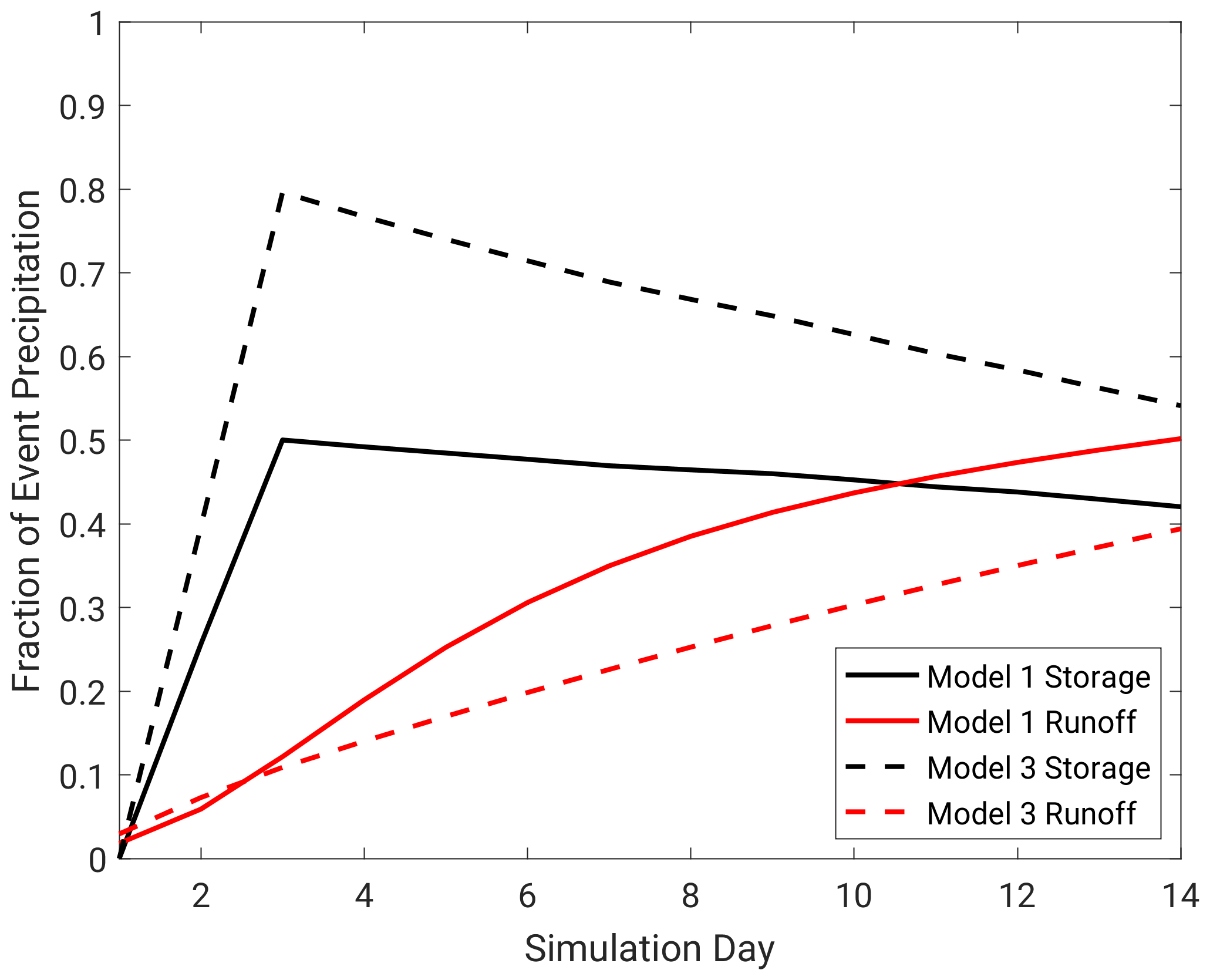
Figure 14Change in storage (black lines) and cumulative runoff (red lines) normalized by flood event precipitation input for model 1 (solid) and model 3 (dashed) at Island Park for one precipitation frequency distribution bin, using the median (50th percentile) precipitation frequency distribution.
Differences in model total storage and subsequent runoff generation drive the different flood responses across both basins. Figure 14 shows the average model response for models 1 (HEC-HMS) and 3 (SAC-SMA) for a subset of precipitation event forcings for Island Park. The change in storage and cumulative runoff are normalized by the total precipitation input to highlight storage and runoff efficiency differences between the two models. Note the precipitation input occurs on days 1 and 2. Models with high event-based runoff ratios generate runoff more readily and have smaller subsurface storages, while models with lower flood event runoff ratios allow for more infiltration and storage. Model 3 stores about 60 % more of the precipitation event than model 1 and ends up generating 25 % less cumulative runoff than model 1. These differences are more important for basins using an integrated flood metric, such as Island Park here, as responsive models generate larger volumes, while the other models store more of the precipitation event forcing and release it over longer periods of time. This point should be the focus of additional study and provides one physical process comparison to identify the appropriate model structures for a given basin. While the focus of this study was on stochastic rainfall–runoff modeling for FF studies, there are potentially broader applications to hydrologic modeling for any purpose, including planning, design, or restoration often focused on more frequent floods up to extreme ones for risk analysis. For example, stochastic rainfall–runoff modeling is data and labor intensive, thus less intensive methods are frequently used, most commonly AEP-neutral assumptions of the precipitation return period being equal to the flood return period. Even in those studies, model selection, parameterization, initial conditions, calibration, and forcing still play an important role in model outcome. Additionally, examining a range of return periods rather than just extreme floods was intentional to help inform a broader range of applications beyond those focused on risk for large dams where only extreme floods are relevant. Understanding of the sensitivity in rainfall–runoff modeling, whether stochastic or not, is important for flood studies. The results of this study can help guide model selection and development and provide a better understanding of variance in a variety of flood studies.
The key generalizable conclusions are as follows:
-
ICs and precipitation frequency distributions contribute the most variance in the stochastic flood modeling chain for frequent and extreme floods, respectively.
-
Hydrological model structure can be equally important, particularly for multi-day volume flood metrics. This highlights the need to critically assess assumptions underpinning models, understand basin flood generation processes, and develop methods to select appropriate models. This includes the re-examination of the AEP-neutral assumption and shifting to model process parameterizations that are most plausible for the study catchment.
-
Model parameter and model structure–parameter interactions can be important if the model parameter space is not well constrained during calibration.
-
Confirming many other studies (e.g., Gupta et al., 2009; Mizukami et al., 2019), the Kling–Gupta efficiency (KGE) results in better hydrologic model performance than NSE (or RMSE) for the calibration of extreme events and volume-integrated flood metrics and is more flexible for application-specific uses through the use of user-specified component weights.
The FUSE model is available at https://doi.org/10.5281/zenodo.5567163 (Newman et al., 2021).
The watershed characteristics, reconstructed flow data, and precipitation frequency estimates are available on request from the United States Bureau of Reclamation. The FUSE model output data are available at https://data.usbr.gov/catalog/4421 (Newman et al., 2020).
All authors contributed to the experimental design. AJN and MS performed the computations, while AJN, AGS, and KDH prepared the figures and tables. AJN led preparation of the paper with contributions from all authors.
The contact author has declared that neither they nor their co-authors have any competing interests.
Publisher’s note: Copernicus Publications remains neutral with regard to jurisdictional claims in published maps and institutional affiliations.
This work was partially supported by the National Center for Atmospheric Research, which is a major facility sponsored by the National Science Foundation (grant no. 1852977). We gratefully acknowledge high-performance computing support from Cheyenne (https://doi.org/10.5065/D6RX99HX), provided by NCAR's Computational and Information Systems Laboratory and sponsored by the National Science Foundation. We also thank the two anonymous reviewers and Daniel Wright, for their helpful review comments which improved the paper.
This research has been supported by the Bureau of Reclamation (grant no. R16AC00039) and the National Science Foundation (grant no. 1852977).
This paper was edited by Elena Toth and reviewed by Daniel Wright and two anonymous referees.
Addor, N., Rossler, O., Koplin, N., Huss, M., Weingartner, R., and Seibert, J.: Robust changes and sources of uncertainty in the projected hydrological regimes of Swiss catchments, Water Resour. Res., 50, 7541–7562, https://doi.org/10.1002/2014WR015549, 2014.
Anderson, E. A.: Calibration of conceptual hydrologic models for use in river forecasting, Office of Hydrologic Development, US National Weather Service, Silver Spring, MD, 2002.
Arnaud, P., Cantet P., and Odry, J.: Uncertainties of flood frequency estimation approaches based on continuous simulation using data resampling, J. Hydrol., 554, 360–369, 2017.
Bell, F. C.: The areal reduction factors in rainfall-frequency estimation, Natural Environmental Research Council, Report 35, Institute of Hydrology, Wallingford, United Kingdom, 1976.
Bennett, T. H.: Development and application of a continuous soil moisture accounting algorithm for the Hydrologic Engineering Center Hydrologic Modeling System (HEC-HMS), University of California, Davis, 1998.
Blazkova, S. and Beven, K.: A limits of acceptability approach to model evaluation and uncertainty estimation in flood frequency estimation by continuous simulation: Skalka catchment, Czech Republic, Water Resour. Res., 45, W00B16, https://doi.org/10.1029/2007WR006726, 2009.
Bosshard, T., Carambia, M., Goergen, K., Kotlarski, S., Krahe, P., Zappa, M., and Schär, C.: Quantifying uncertainty sources in an ensemble of hydrological climate-impact projections, Water. Resour. Res., 49, 1523–1536, https://doi.org/10.1029/2011WR011533, 2013.
Boughton, W. and Droop, O.: Continuous simulation for design flood estimation – a review, Environ. Modell. Softw., 18, 309–318, 2003.
Breuer, L., Gosling, S. N., Yang, T., Hoffmann, P., Hattermann, F. F., Krysnaova, V., Wada, Y., Su, B., Masaki, Y., Müller, C., Daggupati, P., Stacke, T., Fekete, B., Motovilov, Y., Vetter, T., Flörke, F., Liersch, S., Donnelly, C., and Samaniego, L.: Sources of uncertainty in hydrological climate impact assessment: a cross-scale study, Environ. Res. Lett., 13, 015006, https://doi.org/10.1088/1748-9326/aa9938, 2017.
Calver, A., Lamb, R., and Morris, S. E.: River flood frequency estimation using continuous runoff modelling, Proc. Inst. Civ. Eng. Water Marit. Energy, 136, 225–234, 1999.
Chegwidden, O. S., Nijssen, B., Rupp, D. E., Arnold, J. R., Clark, M. P., Hamman, J. J., Kao, S. C., Mao, Y., Mizukami, N., Mote, P. W., Pan, M., Pytlak, E., and Xiao, M.: How Do Modeling Decisions Affect the Spread Among Hydrologic Climate Change Projections? Exploring a Large Ensemble of Simulations Across a Diversity of Hydroclimates, Earth's Futur., 7, 623–637, https://doi.org/10.1029/2018EF001047, 2019.
Clark, M. P., Slater, A. G., Rupp, D. E., Woods, R. A., Vrugt, J. A., Gupta, H. V., Wagener, T., and Hay, L. E.: Framework for Understanding Structural Errors (FUSE): A modular framework to diagnose differences between hydrological models, Water Resour. Res., 44, W00B02, https://doi.org/10.1029/2007WR006735, 2008.
Clark, M. P., Vogel, R. M., Lamontagne, J. R., Mizukami, N., Knoben, W. J., Tang, G., Gharari, S., Freer, J. E., Whitfield, P. H., Shook, K., and Papalexiou, S.: The abuse of popular performance metrics in hydrologic modeling, Water Resour. Res., 57, e2020WR029001, https://doi.org/10.1029/2020WR029001, 2021.
Duan, Q. Y., Gupta, V. K., and Sorooshian, S.: Shuffled complex evolution approach for effective and efficient global minimization, J. Optimiz. Theory App., 76, 501–521, 1993.
England Jr., J. E., Godaire, J. E., Klinger, R. E., Bauer, T. R., and Julien, P. Y.: Paleohydrologic bounds and extreme flood frequency of the Upper Arkansas River, Colorado, USA, Geomorphology, 124, 1–16, 2010.
England Jr., J. E., Julien, P. Y., and Velleux, M. L.: Physically-based extreme flood frequency with stochastic storm transposition and paleoflood data on large watersheds, J. Hydrol., 510, 228–245, 2014.
Franchini, M., Hashemi, A. M., and O’Connell, P. E.: Climatic and basin factors affecting the flood frequency curve: PART II – A full sensitivity analysis based on the continuous simulation approach combined with a factorial experimental design, Hydrol. Earth Syst. Sci., 4, 483–498, https://doi.org/10.5194/hess-4-483-2000, 2000.
Gupta, H. V., Kling, H., Yilmaz, K. K., and Martinez, G. F.: Decomposition of the mean squared error and NSE performance criteria: Implications for improving hydrological modelling, J. Hydrol, 377, 80–91, 2009.
Gupta, H. V., Clark, M. P., Vrugt, J. A., Abramowitz, G., and Ye, M.: Towards a comprehensive assessment of model structural adequacy, Water Resour. Res., 48, W08301, https://doi.org/10.1029/2011WR011044, 2012.
Hansen, E. M., Schreiner, L. C., and Miller, J. F.: Application of Probable Maximum Precipitation Estimates, United States East of the 105th Meridian, Hydrometeorological Report No. 52, National Weather Service, National Oceanic and Atmospheric Administration, U.S. Department of Commerce, Silver Spring, MD, 168, 1982.
Hansen, E. M., Fenn, D. D., Schreiner, L. C., Stodt, R. W., and Miller, J. F.: Probable Maximum Precipitation Estimates United States between the Continental Divide and the 103rd Meridian, Hydrometeorological Report No. 55A, National Weather Service, National Oceanic and Atmospheric Administration, U.S. Department of Commerce, Silver Spring, MD, 242, 1988.
Hansen, E. M., Fenn, D. D., Corrigan, P., Vogel, J. L., Schreiner, L. C., and Stodt, R. W.: Probable Maximum Precipitation-Pacific Northwest States, Columbia River (including portions of Canada), Snake River and Pacific Coastal Drainages, Hydrometeorological Report No. 57, National Weather Service, National Oceanic and Atmospheric Administration, U.S. Department of Commerce, Silver Spring, MD, 338, 1994.
Hashemi, A. M., Franchini, M., and O’Connell, P. E.: Climatic and basin factors affecting the flood frequency curve: PART I – A simple sensitivity analysis based on the continuous simulation approach, Hydrol. Earth Syst. Sci., 4, 463–482, https://doi.org/10.5194/hess-4-463-2000, 2000.
Hawkins, E. and Sutton, R.: The Potential to Narrow Uncertainty in Regional Climate Predictions, Bull. Am. Meteorol. Soc., 90, 1095–1107, https://doi.org/10.1175/2009BAMS2607.1, 2009.
Henn, B., Clark, M. P., Kavetski, D., and Lundquist, J. D.: Estimating mountain basin-mean precipitation from streamflow using Bayesian inference, Water Resour. Res., 51, 8012–8033, 2015.
Hosking, J. R. M. and Wallis, J. R.: Paleoflood hydrology and flood frequency analysis, Water Resour. Res., 22, 543–550, 1986.
Hosking, J. R. M. and Wallis, J. R.: Regional Frequency Analysis, Cambridge University Press, Cambridge, UK, 244 pp., https://doi.org/10.1017/CBO9780511529443, ISBN 9780511529443, 1997.
Hu, L., Nikolopoulos, E. I., Marra, F., and Anagnostou, E. N.: Sensitivity of flood frequency analysis to data record, statistical model, and parameter estimation methods: An evaluation over the contiguous United States, J. Flood Risk Manage., 13, e12580, https://doi.org/10.1111/jfr3.12580, 2020.
Ivancic, T. J. and Shaw, S. B.: Examining why trends in very heavy precipitation should not be mistaken for trends in very high river discharge, Climatic Change, 133, 681–693, https://doi.org/10.1007/s10584-015-1476-1, 2015.
Jakeman, A. J. and Hornberger, G. M.: How much complexity is warranted in a rainfall-runoff model?, Water. Resour. Res., 29, 2637–2649, 1993.
Klemes, V.: Tall tales about tails of hydrological distributions. I, J. Hydrol. Eng., 5, 227–231, 2000.
Knoben, W. J. M., Freer, J. E., Fowler, K. J. A., Peel, M. C., and Woods, R. A.: Modular Assessment of Rainfall–Runoff Models Toolbox (MARRMoT) v1.2: an open-source, extendable framework providing implementations of 46 conceptual hydrologic models as continuous state-space formulations, Geosci. Model Dev., 12, 2463–2480, https://doi.org/10.5194/gmd-12-2463-2019, 2019.
Kuczera, G., Lambert, M. F., Heneker, T. M., Jennings, S., Frost, A., and Coombes, P.: Joint probability and design storms at the Crossroads, Australian Journal of Water Resources, 10, 63–79, 2006.
Kidson, R. and Richards, K. S.: Flood frequency analysis: assumptions and alternatives, Prog. Phys. Geog., 29, 392–410, 2005.
Lehner, F., Deser, C., Maher, N., Marotzke, J., Fischer, E. M., Brunner, L., Knutti, R., and Hawkins, E.: Partitioning climate projection uncertainty with multiple large ensembles and CMIP5/6, Earth Syst. Dynam., 11, 491–508, https://doi.org/10.5194/esd-11-491-2020, 2020.
Liang, X., Lettenmaier, D. P., Wood, E. F., and Burges, S. J.: A simple hydrologicallybased model of land surface water and energy fluxes for general circulation models, J. Geophys. Res., 99, 14415–14428, 1994.
Markstrom, S. L., Hay, L. E., and Clark, M. P.: Towards simplification of hydrologic modeling: identification of dominant processes, Hydrol. Earth Syst. Sci., 20, 4655–4671, https://doi.org/10.5194/hess-20-4655-2016, 2016.
Mendoza, P. A., Clark, M. P., Mizukami, N., Newman, A. J., Barlage, M., Gutmann, E. D., Rasmussen, R. M., Rajagopalan, B., Brekke, L. D., and Arnold, J. R.: Effects of hydrologic model choice and calibration on the portrayal of climate change impacts, J. Hydrometeorol, 16, 762–780, 2015.
Merz, B. and Thieken, A. H.: Separating natural and epistemic uncertainty in flood frequency analysis, J. Hydrol., 309, 114–132, 2005.
Merz, B. and Thieken, A. H.: Flood risk curves and uncertainty bounds, Nat. Hazards, 51, 437–458, 2009.
Mizukami, N., Rakovec, O., Newman, A. J., Clark, M. P., Wood, A. W., Gupta, H. V., and Kumar, R.: On the choice of calibration metrics for “high-flow” estimation using hydrologic models, Hydrol. Earth Syst. Sci., 23, 2601–2614, https://doi.org/10.5194/hess-23-2601-2019, 2019.
Murphy, A. H.: Skill scores based on the mean square error and their relationships to the correlation coefficient, Mon. Weather Rev., 116, 2417–2424, 1988.
National Research Council: Estimating Probabilities of Extreme Floods: Methods and Recommended Research, National Academy Press, Washington, D.C., 160 pp., https://doi.org/10.17226/18935, 1988.
Nathan, R., Weinmann, E., and Hill, P.: Use of Monte Carlo simulation to estimate the expected probability of large to extreme floods, The Institute of Engineers Australia, 28th International Hydrology and Water Resources Symposium, Wollongong, NSW, 10–14 November, 2003.
Newman, A. J., Clark, M. P., Craig, J., Nijssen, B., Wood, A., Gutmann, E., Mizukami, N., Brekke, L. D., and Arnold, J. R.: Gridded ensemble precipitation and temperature estimates for the contiguous United States, J. Hydrometeorol., 16, 2481–2500, 2015.
Newman, A. J., Mizukami, N., Clark, M. P., Wood, A. W., Nijssen, B., and Nearing, G.: Benchmarking of a physically based hydrologic model, J. Hydrometeorol., 18, 2215–2225, 2017.
Newman, A. J., Stone, A. G., Saharia, M., and Holman, K. D.: Data and Report from S&T Project 1794: Identifying Sources of Uncertainty in Flood Frequency Analyses, U.S. Dept. of the Interior, Bureau of Reclamation, Reclamation Information Sharing Environment (RISE) [data set], available at: https://data.usbr.gov/catalog/4421 (last access: 13 October 2021), 2020.
Newman, A. J., Clark, M. P., Addor, N., Kavetski, D., and Henn, B.: Framework for Understanding Structural Errors (FUSE) with user specified initial states, Zenodo [code], https://doi.org/10.5281/zenodo.5567163, 2021.
Packman, J. and Kidd, C.: A logical approach to the design storm concept, Water Resour. Res., 16, 994–1000, 1980.
Paquet, E., Garavaglia, F., Garçon, R., and Gailhard, J.: The SCHADEX method: A semi-continuous rainfall–runoff simulation for extreme flood estimation, J. Hydrol., 495, 23–37, 2013.
Pathiraja, S., Westra, S., and Sharma, A.: Why continuous simulation? The role of antecedent moisture in design flood estimation, Water Resour. Res., 48, W06534, https://doi.org/10.1029/2011WR010997, 2012.
Peleg, N., Blumensaat, F., Molnar, P., Fatichi, S., and Burlando, P.: Partitioning the impacts of spatial and climatological rainfall variability in urban drainage modeling, Hydrol. Earth Syst. Sci., 21, 1559–1572, https://doi.org/10.5194/hess-21-1559-2017, 2017.
Rahman, A., Weinmann, P. E., Hoang, T. M. T., and Laurenson, E. M.: Monte Carlo simulation of flood frequency curves from rainfall, J. Hydrol., 256, 196–210, https://doi.org/10.1016/S0022-1694(01)00533-9, 2002.
Reclamation (Bureau of Reclamation): Altus Dam Hydrologic Hazard and Reservoir Routing for Corrective Action Study. W.C. Austin Project, OK, Billings, MT. U.S. Dept. of the Interior, Bureau of Reclamation Great Plains Region, 230 pp., 2012.
Reclamation (Bureau of Reclamation): Island Park Dam Meteorology for Application in Hydrologic Hazard Analysis, Minidoka Project, ID, Boise, ID. U.S. Dept. of the Interior, Bureau of Reclamation Pacific Northwest Region, 88 pp., 2016a.
Reclamation (Bureau of Reclamation): Island Park Dam Hydrologic Hazard for Issue Evaluation, Minidoka Project, ID, Boise, ID, U.S. Dept. of the Interior, Bureau of Reclamation Pacific Northwest Region, 74 pp., 2016b.
Reclamation (Bureau of Reclamation): Unity Dam Hydrologic Hazard for Issue Evaluation. Burnt River Project, Oregon, Boise, ID, U.S. Dept. of the Interior, Bureau of Reclamation Pacific Northwest Region, Technical Memorandum 8250-2018-002, 284 pp., 2018.
Schaefer, M. G. and Barker, B. L.: Stochastic Event Flood Model (SEFM), in: Mathematical Models of Small Watershed Hydrology and Applications, edited by: Singh, V. J., 950 pp., Highlands Ranch, Colorado, USA, ISBN 9781887201353, 2002.
Schreiner, L. C. and Riedel, J. T.: Probable Maximum Precipitation Estimates, United States East of the 105th Meridian, Hydrometeorological Report No. 51, National Weather Service, National Oceanic and Atmospheric Administration, U.S. Department of Commerce, Silver Spring, MD, 87 pp., 1978.
Sharma, A., Wasko, C., and Lettenmaier, D. P.: If precipitation extremes are increasing, why aren't floods?, Water Resour. Res., 54, 8545–8551, https://doi.org/10.1029/2018WR023749, 2018.
Small, D., Islam, S., and Vogel, R. M.: Trends in precipitation and streamflow in the eastern US: Paradox or perception?, Geophys. Res. Lett., 33, L03403, https://doi.org/10.1029/2005GL024995, 2006.
Stedinger, J. R., Vogel, R. M., and Foufoula-Georgiou, E.: Frequency analysis of extreme events, in: Handbook of Hydrology, edited by: Maidment, D., 1st edition, 1424 pp., McGraw-Hill, New York, ISBN 13 978 0070397323, 1993. 13 978 0070397323
Swain, R. E., England, J. F., Bullard, K. L., Raff, D. A., and United States.: Guidelines for evaluating hydrologic hazards, Denver, CO, U.S. Dept. of the Interior, Bureau of Reclamation, 91 pp., 2006.
Tijms, H. C.: A first course in stochastic models, John Wiley and Sons, 448 pp., West Sussex, England, ISBN 13 978 0471498803, 2003. 13 978 0471498803
Wright, D. B., Smith, J. A., and Baeck, M. L.: Flood frequency analysis using radar rainfall fields and stochastic storm transposition, Water Resour. Res., 50, 1592–1615, https://doi.org/10.1002/2013WR014224, 2014.
Wright, D. B., Yu, G., and England, J. F.: Six decades of rainfall and flood frequency analysis using stochastic storm transposition: Review, progress, and prospects, J. Hydrol., 585, 124816, https://doi.org/10.1016/j.jhydrol.2020.124816, 2020.
Yu, G., Wright, D. B., Zhu, Z., Smith, C., and Holman, K. D.: Process-based flood frequency analysis in an agricultural watershed exhibiting nonstationary flood seasonality, Hydrol. Earth Syst. Sci., 23, 2225–2243, https://doi.org/10.5194/hess-23-2225-2019, 2019.
Zhu, Z., Wright, D. B., and Yu, G.: The impact of rainfall space-time structure in flood frequency analysis, Water Resour. Res., 54, 8983–8998, https://doi.org/10.1029/2018WR023550, 2018.