Benchmarking data-driven rainfall–runoff models in Great Britain: a comparison of long short-term memory (LSTM)-based models with four lumped conceptual models

Long short-term memory (LSTM) models are recurrent neural networks from the field of deep learning (DL) which have shown promise for time series modelling, especially in conditions when data are abundant. Previous studies have demonstrated the applicability of LSTM-based models for rainfall–runoff modelling; however, LSTMs have not been tested on catchments in Great Britain (GB). Moreover, opportunities exist to use spatial and seasonal patterns in model performances to improve our understanding of hydrological processes and to examine the advantages and disadvantages of LSTM-based models for hydrological simulation. By training two LSTM architectures across a large sample of 669 catchments in GB, we demonstrate that the LSTM and the Entity Aware LSTM (EA LSTM) models simulate discharge with median Nash–Sutcliffe efficiency (NSE) scores of 0.88 and 0.86 respectively. We find that the LSTM-based models outperform a suite of benchmark conceptual models, suggesting an opportunity to use additional data to refine conceptual models. In summary, the LSTM-based models show the largest performance improvements in the north-east of Scotland and in south-east of England. The south-east of England remained difficult to model, however, in part due to the inability of the LSTMs configured in this study to learn groundwater processes, human abstractions and complex percolation properties from the hydro-meteorological variables typically employed for hydrological modelling.

1 Introduction

Rainfall–runoff models have evolved over many decades, reflecting a diversity of applications and purposes. These models range from physically based, spatially explicit models such as SHETRAN (Birkinshaw et al., 2010), CLASSIC (Crooks et al., 2014) and PARFLOW (Maxwell et al., 2009) to lumped conceptual models such as TOPMODEL (Beven and Kirkby, 1979) and VIC (Liang, 1994). Additionally, data-driven models have also been used for modelling rainfall–runoff processes (Reichstein et al., 2019; Elshorbagy et al., 2010; Wilby et al., 2003; Nourani et al., 2014; Le et al., 2019; Gauch et al., 2021b). The diversity of modelling approaches reflects the diversity of user objectives, uncertainty in terms of how to best represent the stores and fluxes of water and energy, and the trade-offs in terms of data requirements, degree of realism and computational costs (Beven, 2011).

Data-driven models range from simple regression models to large neural networks with thousands of parameters. These methods draw on empirical relationships between inputs and outputs to form a representation of how the hydrological system operates more generally (Beven, 2011). Other approaches from the class of data-driven models, such as statistical modelling and machine learning, include genetic programming (Chadalawada et al., 2020; Herath et al., 2021), random forests (Booker and Woods, 2014) and support vector regression models (Elshorbagy et al., 2010). Alternative empirical approaches also exist, including data-based mechanistic (DBM) modelling (Young, 1998, 2003). DBM approaches suggest that rather than imposing model structures from the outset hydrologists should in the first instance allow the data to suggest an appropriate model structure. Then, the modeller should see if there is a mechanistic interpretation of the learnt model structure (Young and Beven, 1994). Our modelling approach uses deep learning (DL) techniques, which have produced accurate predictions on a wide variety of tasks, including rainfall–runoff modelling (Huntingford et al., 2019), and represent a fruitful area of further exploration for hydrologists and Earth scientists (Reichstein et al., 2019). For a more complete picture on the uses of DL techniques in hydrology, an interested reader is referred to Shen (2018), Beven (2020), Nearing et al. (2020), and Kratzert et al. (2018).

DL methods have been used in hydrology and meteorology for decades (Daniell, 1991; Halff et al., 1993; Dawson and Wilby, 1998; Wilby et al., 2003; Peel and McMahon, 2020). However, one architecture explicitly designed for time series simulation, the long short-term memory (LSTM) network (Hochreiter et al., 2001; Hochreiter, 1991), has recently demonstrated credible performance for modelling hydrological signatures across the continental United States (CONUS) (Kratzert et al., 2018, 2019; Duan et al., 2020; Feng et al., 2020; Gauch et al., 2021b; Fang et al., 2018, 2020). More recent work has begun not only to explore the accuracy of forecasts but also to use LSTMs to (i) provide estimates of uncertainty (Klotz et al., 2020), (ii) explore the ability of the LSTM to integrate prior physical knowledge into DL model architectures (Hoedt et al., 2021; Jiang et al., 2020), and (iii) to use LSTMs to produce predictions at multiple timescales from a single model (Gauch et al., 2021a).

By contrast with the physically based, spatially explicit hydrological models, lumped conceptual models have relatively few parameters and simulate the stores and fluxes of water on a catchment scale, e.g. using a single store to represent the catchment-wide upper-soil water storage (Beven, 2011). Lumped conceptual models have lower data and computational requirements when compared to the spatially explicit, physically based, models, which is one reason why they are often used for operational purposes (Clark et al., 2008). There exist many lumped conceptual models, differing in their internal structures, the equations that govern fluxes of water and energy, and the processes that are included (Knoben et al., 2019). As an evidence-guided discipline, performance benchmarks provide hydrologists with an objective means for selecting between different models, instead of model selection by lineage or affiliation (Addor and Melsen, 2019). Furthermore, when applied over a large sample of catchments, differences in model performance can be instructive with regards to the hydrological conditions that are well simulated by one model compared with others (Gupta et al., 2014). Increasingly, “we need large-scale evaluations of model capability to identify which processes are important and which model structure(s) are most appropriate” (Lane et al., 2019, p. 4012).

This paper seeks to address three research gaps. First, there exists no large-sample performance benchmark of LSTMs in a Great Britain (GB) context. This is important because scientists and practitioners are interested in using LSTMs as hydrological models for hazard impact assessment, hazard early warning and rainfall–runoff modelling (Shen, 2018). Therefore, a rigorous assessment of LSTM performances is necessary to determine whether such a model choice is appropriate in the GB context. Furthermore, given that the data archives are rich in GB, there exists a very good opportunity to learn more about the capabilities and limitations of LSTM-based methods (Clark and Khatami, 2021). Second, there exists only one other comparison of the EA LSTM performance against the LSTM (Kratzert et al., 2019). Finally, there exist no studies that explore the relationship of performance differences (between conceptual and deep learning models) with the hydrological conditions in which those differences occur. The aim of studying the relationship between performance differences and hydrological conditions is to determine how best to improve our conceptual models. What information might be present in the underlying data that can help identify processes that are currently missing from our conceptual models?

The research questions that this study seeks to address are determined by the research gaps identified above.

1. How well do LSTM-based models (including the EA LSTM) simulate discharge in Great Britain?

2. How do LSTM-based model performances compare with the conceptual models used as a benchmark?

3. Can we extract information from the spatial and temporal patterns in diagnostic measures? For example, what is the relationship between LSTM performance and catchment attributes?

To address these questions, we have trained an ensemble of eight LSTMs and eight EA LSTMs on 669 catchments in Great Britain. We compare the results of the LSTM models with four deterministic lumped-conceptual models from a previous benchmarking study (Lane et al., 2019). This paper provides an evaluation of LSTM model ability across a large sample of GB catchments. We explore the association between catchment characteristics and the differences in model performances and present a data-driven benchmark that reflects the null-hypothesis of what information is present in a large-sample dataset (Nearing et al., 2020). Future modelling efforts may seek to assess whether hydrological theories encoded in conceptual and process-based models may contain more information than the benchmarks provided here (Nearing et al., 2021).

We believe that the research addresses the following needs of the hydrological community: (i) practitioners wishing to know whether the LSTM is a justifiable model choice in the GB context, (ii) scientists and practitioners interested in understanding under what hydrological conditions (e.g. catchment attributes) the LSTM performance differs from conceptual models, and (iii) as a reference for future GB-wide modelling studies.

2 Methods

2.1 Data – CAMELS-GB

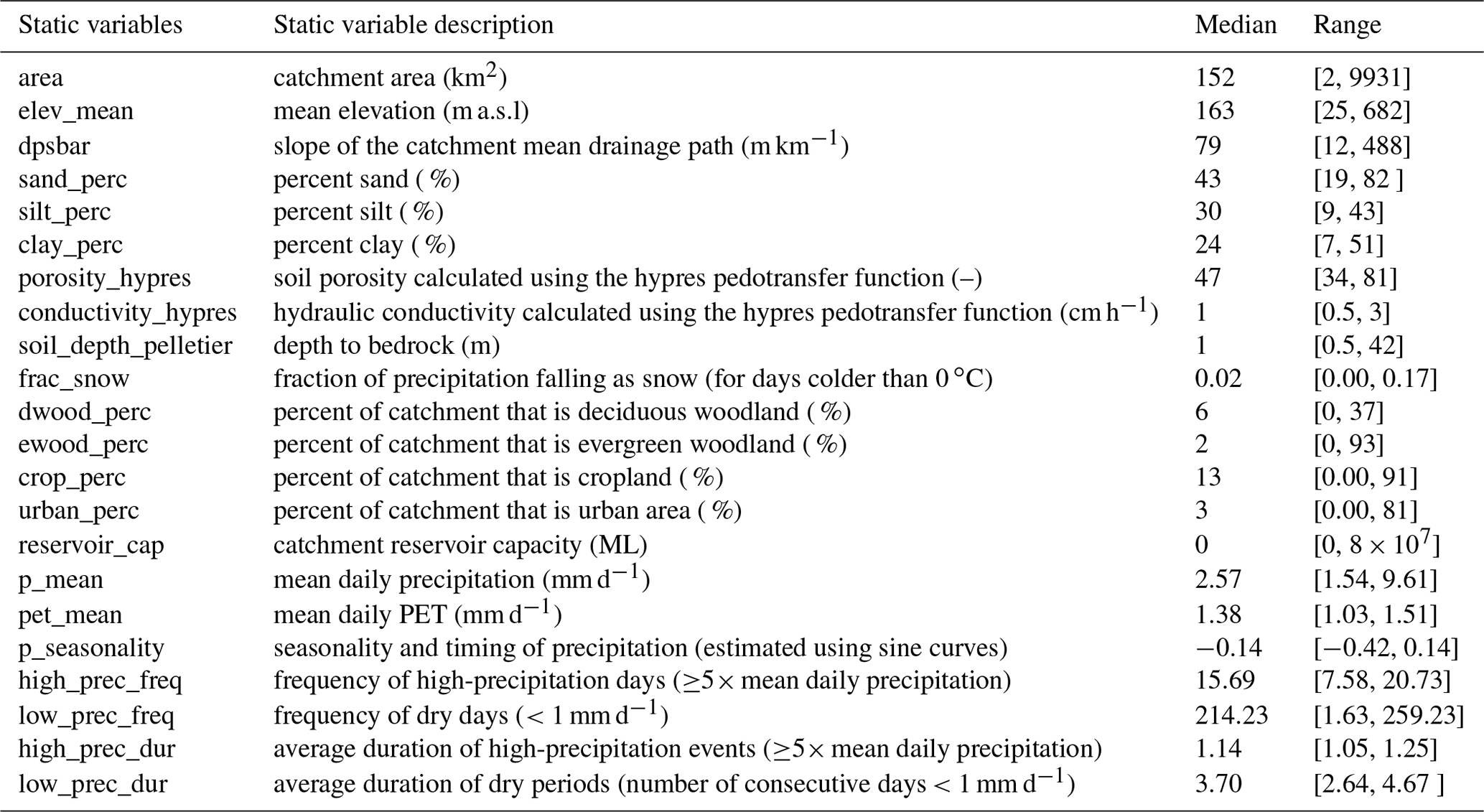
All data employed in this analysis originate from the CAMELS-GB data (Coxon et al., 2020a). CAMELS-GB is a recently released, large-sample, long-term, daily dataset that offers the potential for GB-wide modelling studies. CAMELS-GB collates hydrologically relevant data for 671 GB catchments between the years of 1970 and 2015. The dataset includes daily time series for meteorology (dynamic data – X_t,n) and discharge (target data – y_t,n). Also included are catchment attributes (static data – A_t,n) such as topography, climate, hydrologic signatures, soil and land cover, hydrogeology, and human influence. These features are, in reality, not static over time. However, for the purposes of this study we treat these features as time-invariant. Further information on the variables we used as input to our model can be found in Table 1. The reader is directed to Coxon et al. (2020b) for details of the source of the data, how the data were processed and a discussion of data limitations.

The dataset contains novel inputs compared with previous CAMELS (US, Chile, Brazil) datasets (Addor et al., 2017; Alvarez-Garreton et al., 2018; Chagas et al., 2020), such as human attributes, calculated potential evapotranspiration (pet) and uncertainty estimates. We do not use all of these features here. The static attributes we use to train the LSTM models are listed in Table 1. These static attributes were chosen to reproduce the experimental framework of Kratzert et al. (2019); however, the differences reflect the fact that the CAMELS-US and CAMELS-GB have slightly different attributes. These include both catchment properties and climate properties, describing the conditions relevant for rainfall–runoff modelling in different catchments.

Table 1 Catchment attributes from the CAMELS-GB dataset (Coxon et al., 2020b) used to train the LSTM-based models and the static features included in A.

2.2 An overview of the LSTM and EA LSTM

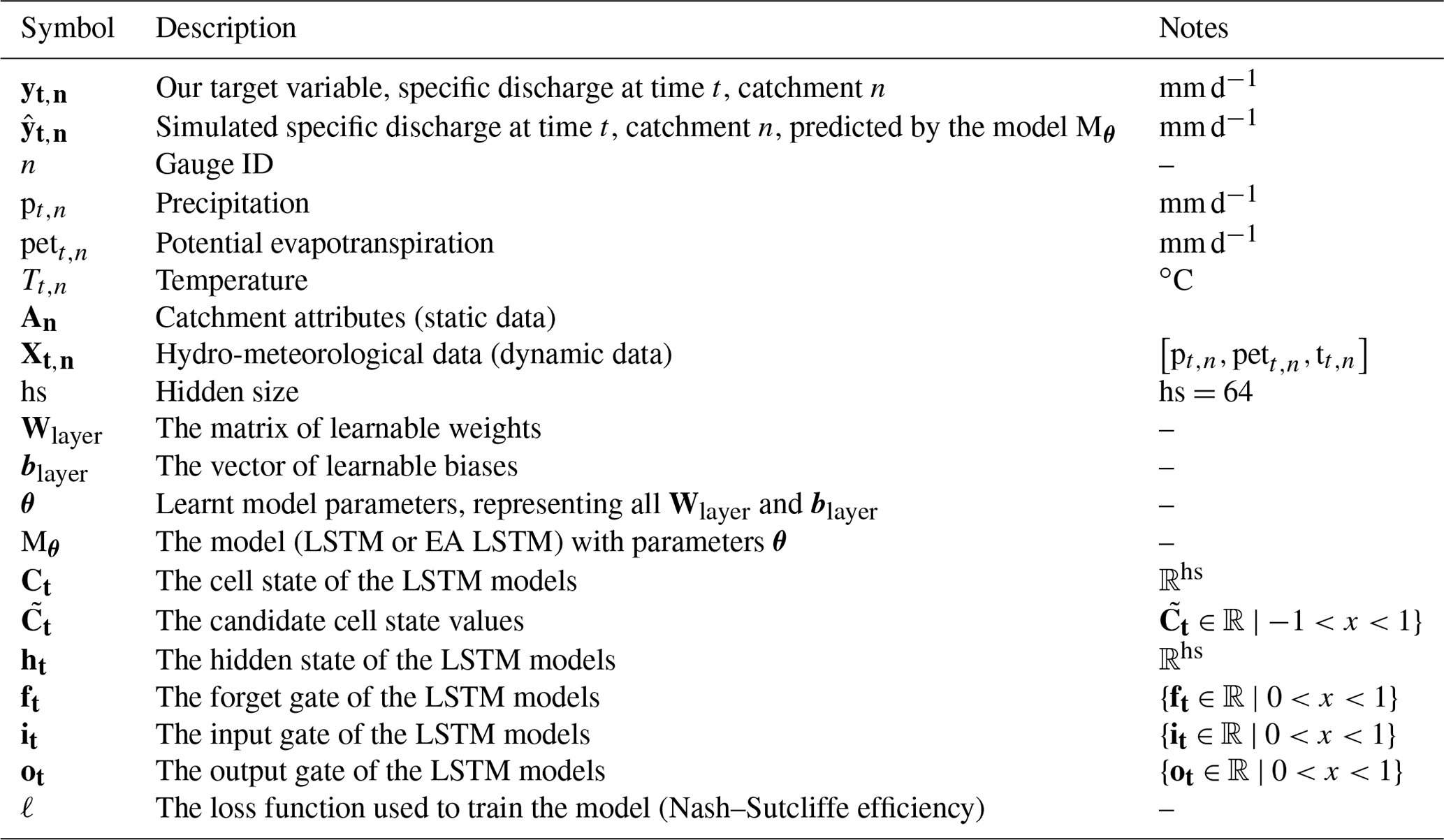
In this paper, we test two neural network architectures used in other hydrological studies (Shen et al., 2018; Kratzert et al., 2019). The first is the LSTM, which has been used in a variety of time series modelling applications. The second model is the EA LSTM, which conditions the discharge response to meteorological forcings on time-invariant properties of river catchments, such as soil and topographic attributes, treating these time-invariant properties separately. For a summary of notation used throughout the paper, please refer to Table 2:

Table 2 Table describing the notation used throughout the paper.

What follows is a brief introduction to the LSTM model architectures. For a more complete description of these models please refer to the Sect. S1 in the Supplement and Kratzert et al. (2018, 2019).

The LSTM has a strong inductive bias towards retaining information over long sequences (Hochreiter, 1991; Bengio et al., 1994). This means that the LSTM architecture is designed to retain information that is important over both long- and short-term time horizons. LSTMs do this by maintaining two state vectors: a cell memory vector that captures slowly evolving processes (C_t) and a more quickly evolving state vector, colloquially named the “hidden” vector (h_t). Information flow is controlled by a series of gates which are neural network layers that determine what information is removed from f_t (forget gate), what information is stored in i_t (input gate) and what information is passed to the o_t (output gate) respectively.

The Entity Aware LSTM (EA LSTM) modifies the forget gate, so the output of the forget gate is a function of only the static catchment attributes (A_n) rather than both the catchment attributes and the dynamic data ($[{\mathbf{X}}_{\mathbf{t},\mathbf{n}},{\mathbf{A}}_{\mathbf{n}}]$). The EA LSTM was developed specifically for rainfall–runoff modelling (Kratzert et al., 2019). For the sake of clarity, it is important to note that both models receive the same information. The LSTM still receives the static catchment attributes. However, rather than affecting only the input gate the static data can influence all gates, since they are appended to a vector of dynamic inputs $\left(\left[{\mathbf{X}}_{\mathbf{t},\mathbf{n}},{\mathbf{A}}_{\mathbf{n}}\right]\right)$, and so the same information is given to the LSTM at each time step. The static attributes are used by the LSTM in the same way as the dynamic data. This offers extra flexibility for the LSTM compared with the EA LSTM, since the LSTM is able to modify the input gate based on information from time-varying data, whereas the EA LSTM is not. We are using the static nature of the data as a constraint on the EA LSTM to reflect the nature of the input data (separated into static and dynamic inputs).

2.3 Model training

We used the “neuralhydrology” codebase, written in Python 3.6 (Van Rossum et al., 2007), to train and evaluate the models, which is found at the following link: https://github.com/neuralhydrology/neuralhydrology (last access: 20 September 2021). The configuration files used to run the models can be found using the links at the end of this article. The predictions and error metrics for the fitted models can be found online at Zenodo (https://doi.org/10.5281/zenodo.4555819).

The goal of rainfall–runoff modelling is to predict time-varying specific discharge, ${\mathbf{y}}_{\mathbf{n}}=({\mathbf{y}}_{\mathbf{1},\mathbf{n}},\mathrm{\dots },{\mathbf{y}}_{\mathbf{T},\mathbf{n}})\in \mathbb{R}{}^T$ (mm d⁻¹) for time $t=\mathit{\{}\mathrm{1},\mathrm{\dots },T\mathit{\}}$ at measuring gauge n of N, given hydro-meteorological forcing data, ${\mathbf{X}}_{\mathbf{n}}=({\mathbf{X}}_{\mathbf{1},\mathbf{n}},\mathrm{\dots },{\mathbf{X}}_{\mathbf{T},\mathbf{n}})$, and catchment attributes (A_n – Table 1) within the catchment area upstream of the gauge. In the present case for GB, N=669. Although the underlying CAMELS-GB data have 671 station gauges, we trained on data from only 669 stations, because two basins have missing data in the static attributes; stations 18011 and 26006 have missing mean elevation (elev_mean) and mean drainage path slope (dpsbar).

Our task is to train a regional hydrological model, i.e. one model for all catchments in the dataset. This means that we learn a single set of parameters, θ, of a model, M_θ, that minimizes the loss function, $\mathrm{\ell }({\widehat{\mathbf{y}}}_{\mathbf{t},\mathbf{n}},{\mathbf{y}}_{\mathbf{n}})$, for all flow gauges and thus accurately simulates discharge (${\widehat{\mathbf{y}}}_{\mathbf{t},\mathbf{n}}$) for all of the basins in our subset of CAMELS-GB:

$$\begin{array}{}\text{(1)}& {\widehat{\mathbf{y}}}_{\mathbf{t},\mathbf{n}}={\mathrm{M}}_{\mathit{\theta }}\left(\left[{\mathbf{A}}_{\mathbf{n}},{\mathbf{X}}_{\mathbf{t}-\mathbf{k}+\mathbf{1},\mathbf{n}},\mathrm{\dots },{\mathbf{X}}_{\mathbf{t},\mathbf{n}}\right];\mathit{\theta }\right).\end{array}$$

We train our model using the Nash–Sutcliffe efficiency (NSE) loss as our objective function (ℓ), as described in Kratzert et al. (2019). Other objective functions could be used; however, we use the same objective function as the conceptual models we compare against, in order to control the possible sources of performance differences. The NSE describes the squared error loss normalized by the total variance of the observations. In order to account for the fact that some basins will have lower variance than others, we follow Kratzert et al. (2019) to normalize by basin-specific variance. This prevents the loss from being overly weighted towards high-variance catchments.

For this study, we trained the models on the days from 1 January 1988 to 31 December 1997 and tested on a hold-out sample using the days from 1 January 1998 to 31 December 2008 (4018 d of test data). We withheld the years 1975 to 1980 from the training process to check the performance of the model during training (our validation set). This means that we have separate time periods for calibration (1988–1997; train period) and evaluation (1998–2008; hold-out test period). These train and test periods were chosen to facilitate the comparison with the study whose published results for four lumped hydrological models we use as a benchmark (Lane et al., 2019). For further analysis of the train and test periods, please see Sect. S2.

Our input data were taken from CAMELS-GB, described above (Coxon et al., 2020b). We used precipitation, potential evapotranspiration and temperature as dynamic inputs (${\mathbf{X}}_{\mathbf{t},\mathbf{n}}=\left[{\mathrm{p}}_{t,n},{\mathrm{pet}}_{t,n},{\mathrm{T}}_{t,n}\right]$). We selected 21 individual features describing each catchment's topographic, soil, land-cover, and climatic properties as static inputs (A_n). These attributes were chosen to reflect hydrological information that the model can use to distinguish between catchment rainfall–runoff behaviours (Kratzert et al., 2019). These catchment attributes are described in Table 1. For both LSTM models, we pass the final hidden output through a fully connected (linear) layer. This final layer maps our hidden state vector to a scalar prediction (${\widehat{\mathbf{y}}}_{\mathbf{t},\mathbf{n}}\in \mathbb{R}$) for discharge at that gauge on that day. We give the models 1 year of daily dynamic data (365 input time steps, $X_n=[{\mathbf{X}}_{\mathbf{t}-\mathbf{365},\mathbf{n}},\mathrm{\dots },{\mathbf{X}}_{\mathbf{t},\mathbf{n}}]$) to predict the final time step of specific discharge (${\widehat{\mathbf{y}}}_{\mathbf{t},\mathbf{n}}$).

All national results shown below are calculated for the 518 gauges that are found in both the CAMELS-GB data and the benchmark data. We then evaluate model performance on all of these basins for our test (evaluation) period (1998–2008). For each model (LSTM, EA LSTM), we also calculate the average of an ensemble of eight individually trained models with different random seeds. This strategy accounts for the random initialization of the network and the stochastic nature of the optimization algorithm. We used a hidden size (hs) of 64 and a final fully connected layer with a dropout rate of 0.4, which aims to avoid overfitting. Dropout works by randomly forcing certain weights in the network to zero (“dropping them out”), forcing the remaining weights to model the discharge without that extra information. This has been found to prevent weights “fixing” the erroneous outputs of other weights, preventing co-adaptation of weights and, ultimately, encouraging the model to use a simpler and more robust representation of rainfall–runoff processes (Srivastava et al., 2014). The hidden size determines the total number of parameters in the model. For the LSTM, there are 23 361 trainable parameters, whereas the EA LSTM has 14 593 trainable parameters. These are trained on data from 669 catchments over 4018 time steps (2 688 042 samples). Note that this is for a regional model and is independent of the number of catchments. Given that we train the LSTM on 669 catchments, we can interpret the LSTM as equivalent to using 35 parameters per catchment, with a median catchment area of 152 km². The EA LSTM has of the order of 22 parameters per catchment. We chose the hyper-parameters (dropout rate, hidden size – hs) based on analysis of the NSE performances, finding that the improvement of further model complexity (increased hidden size) was negligible after a hidden size of 64. The hidden size was also consistent with the choices made in previous studies (Kratzert et al., 2019). We used the Adam optimization algorithm (Kingma and Ba, 2014) and stopped training after 30 epochs, after which there was no further improvement to the model. An epoch reflects a single pass of the training dataset through the model, such that every sample in the training dataset has been used to update the model weights. This reflects the fact that during the training of DL models, the data are often split into batches to allow large datasets to be read into memory. The LSTM ensemble took 10 h to train. The EA LSTM ensemble took 96 h to train. All models were trained on a machine with 188 GB of RAM and a single NVIDIA V100 GPU.

2.4 Model performance comparisons

The LSTMs learn to represent hydrological processes directly from data. When the LSTMs perform well on hold-out test samples, a necessary (but not sufficient) conclusion is that the data contain useful information about the hydrological processes that translate inputs (precipitation) into outputs (discharge). The differences in model performance between the LSTMs and the benchmark hydrological models can be used to determine hydrological processes that are described by the input data but not captured or under-represented by the benchmark hydrological models.

2.4.1 Benchmark models

In order to provide a reference for model performance statistics, we compare the performance of the LSTM-based models against four lumped conceptual models from the FUSE framework (Clark et al., 2008). To be unbiased on the model calibration, we used simulated discharge time series from Lane et al. (2019), who calibrated and evaluated these four conceptual models on 1000 catchments across Great Britain. The four conceptual models used are TOPMODEL (Beven and Kirkby, 1979), Variable Infiltration Capacity (VIC) (Liang, 1994), Precipitation-Runoff Modelling System (PRMS) (Leavesley et al., 1983) and SACRAMENTO (Burnash et al., 1973). These conceptual models are often used in operational settings, due to the relative ease of use and lower data requirements when compared with physically based models. These conceptual models all explicitly maintain mass balance and so assume no losses or gains of water other than flow from the catchment outlet or evaporation.

These conceptual models are all lumped models run at a daily time step. Each model is explicitly forced to close the water balance, limited by an upper limit of potential evapotranspiration for water losses. Every one of the conceptual models has a gamma distribution routing function. Furthermore, the four conceptual models do not include a snow routine nor a vegetation module (Clark et al., 2008). SACRAMENTO has 5 stores and 12 parameters per catchment, both VIC and TOPMODEL have 2 stores and 10 parameters, and PRMS has 3 stores and 11 parameters. A more complete description of these benchmark models and the processes that they include can be found in Table 3 of Lane et al. (2019) and in Sect. 4 of Clark et al. (2008).

The benchmark study provides an assessment of conceptual model simulation performances across a large sample of GB catchments, and it also quantifies uncertainty in hydrological simulations due to parameter uncertainty and model structural uncertainty (Lane et al., 2019). Parameter values for each conceptual model were selected from 10 000 simulations of multi-dimensional parameter space. The best-estimate model parameter values were selected from these 10 000 samples using the Nash–Sutcliffe efficiency score. These best-fit parameters are used as a benchmark against which to compare the LSTM performance. To place the intercomparison into context, we critically reflect on the consistencies and differences between the different model configurations here.

First, the selection of model parameters differs between the LSTM and the conceptual models. The experimental design of the benchmarking study produced 10 000 samples of parameter values, and Lane et al. (2019) provide the simulations given the best fitting parameters for future studies to employ as a benchmark. The LSTM parameters are optimized using stochastic gradient descent, choosing the best fitting set of parameters using the NSE score. While the method of choosing parameters differs, the objective function that determines the “best-fit” parameter values is the same for both the LSTMs and the conceptual models. Second, the calibration and evaluation data are the same. The calibration and evaluation of these models were performed using the same data from CAMELS-GB, i.e. the National River Flow Archive data (Centre for Ecology and Hydrology, 2016) for specific discharge (y_t); the Centre for Ecology and Hydrology Gridded Estimates of Areal Rainfall, CEH-GEAR, for precipitation (Tanguy, 2014); and the Climate Hydrology and Ecology research Support System Potential Evapotranspiration (CHESS-PE) dataset for PET (Robinson et al., 2017). The benchmark experiment selected the best-fitting parameter values using data from the period 1988–2008 and then evaluated their performance on data from 1993–2008 (Lane et al., 2019). Instead, we calibrate the LSTMs on data from 1988–1998 and then evaluate the LSTM performances for our hold-out evaluation period of 1998–2008. We recalculate the performance statistics of the benchmark conceptual models for this evaluation period, 1998–2008, using the published simulated time series. Therefore, the LSTM is evaluated on out-of-sample (in time) data, whereas the conceptual model parameters were calibrated on data included in the evaluation period (in-sample evaluation). Finally, it is worth noting that Lane et al. (2019) focused not only on model performances but also on parameter uncertainty. Uncertainty is an essential component of any modelling study, and our approach of training an ensemble of eight models is one proposed method for dealing with uncertainty in LSTMs. For an analysis of model uncertainty with this method, see Sect. S4. For a more complete treatment and discussion of the different approaches for dealing with uncertainty using LSTMs, see Klotz et al. (2020).

As with any benchmarking study, there are important caveats to the intercomparison of model results. Ultimately, the purpose of the comparison is (i) to provide a reference for the diagnostic measures of LSTM performance, (ii) to identify the hydrological conditions where simulations differ, and (iii) to use these insights to diagnose missing representations in the conceptual models. We agree with Lane et al. (2019) that “benchmark [studies] provide a useful baseline for assessing more complex modelling strategies” (p. 4029), and we follow them in publishing the simulations and results of the LSTM models for future studies to use for comparison.

2.4.2 Evaluation metrics

Each model produces a daily simulated discharge value at each station. Three example hydrographs are shown in Sect. S3. The evaluation metrics described below evaluate the overall performance of each model to reproduce a specific aspect of the observed hydrograph. For the LSTM-based models, the evaluation metrics are calculated given the average discharge of the ensemble. Since no single evaluation metric can fully capture the performance of streamflow simulations across all flow-regimes (Gupta et al., 1998), we use a number of metrics to address the performance of models across the flow regime, outlined below.

We evaluate the goodness-of-fit metrics of the LSTM-based models and the conceptual models using six evaluation metrics. The Nash–Sutcliffe efficiency (NSE) (Nash and Sutcliffe, 1970) score has been used in numerous studies, and there is extensive literature discussing its strengths and weaknesses (Gupta et al., 2009). The NSE can be decomposed into three components: a correlation term, a bias term (BiasError) and a variability (SDError) term (Gupta et al., 2009). The bias term measures the error in predicting the mean flow. The variability term measures the error in predicting the standard deviation of discharge. We report results for the NSE and each of its three components.

To understand how well the LSTMs represent low, mean and high flows, we also consider the biases for different components of the flow duration curve. The low-flow bias (%BiasFLV) is the diagnostic signature measure for long-term base flow (Yilmaz et al., 2008), and low flows are defined as those which are exceeded 70 % of the time. For the middle of the flow duration curve, we use the bias of the midsection of the flow duration curve, between the 20th and 70th percentiles (%BiasFMS). Finally, we also look at the bias of the high flows, considering the top 2 % of flows (%BiasFHV).

3 Results

3.1 National-scale model performance

The LSTM and EA LSTM models produce accurate simulations across Great Britain when evaluated using a variety of metrics, with differing levels of performance improvement over the benchmark conceptual models (See Table 3).

Table 3 Summary of all goodness-of-fit metrics used to benchmark performance against the conceptual models for the validation period 1998–2008 on the 518 stations found in both CAMELS-GB data (Coxon et al., 2020a) and the FUSE conceptual models (Lane et al., 2019). We have shown the median catchment score for the metric given the mean simulated discharge of our ensemble. Values that are not significantly different from the best model are highlighted in bold (α=0.001).

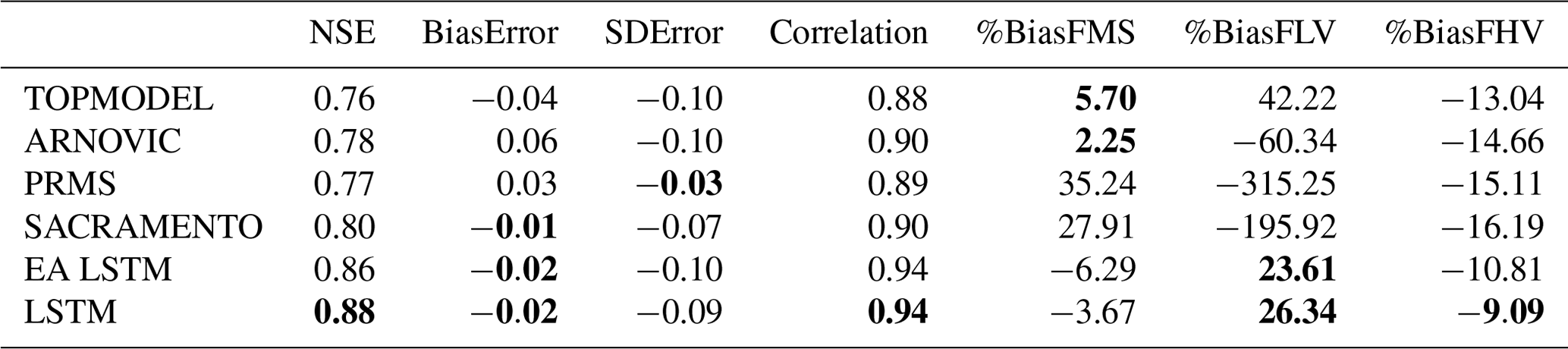
Comparing the median NSE for all catchments, the LSTM ensemble (0.88) outperforms all other models, including the EA LSTM ensemble (0.86). The slightly lower median NSE for the EA LSTM models is consistent with results from previous studies (Kratzert et al., 2019). The CDFs (cumulative distribution functions) of the NSE (Fig. 1a) show the entire distribution of LSTM scores is shifted towards better performances. The LSTM NSE scores are significantly different from all comparison models at α = 0.001 (paired Wilcoxon signed-rank test). We see the same pattern for the EA LSTM models. The performance improvement at the tails is particularly pronounced. Neither the LSTM nor the EA LSTM model have any station gauges with an NSE of less than zero.

As discussed in the methods, we can decompose the NSE into three components: bias (BiasError), correlation and error in predicting the variability of flows (SDError). The pattern of correlation scores closely follows the pattern of NSE, with the entire distribution of catchment correlation scores shifted towards improved performance. The CDFs in Fig. 1c show that the LSTM catchment bias scores are closer to zero than the benchmark models, which reflects the fact that the conceptual models are explicitly mass conserving, whereas the LSTM models are not. The median variability error is negative (Fig. 1d), showing that the LSTMs tend towards underpredicting the variability of flows.

The LSTM shows a large performance improvement for low-flow bias score (%BiasFLV – Fig. 1e). The LSTM has lower median bias in the slope of the midsection of the flow duration curve (%BiasFMS) than all models except ARNOVIC. When we consider the CDFs, both LSTMs have shorter tails than the conceptual models, showing that a greater proportion of catchments have biases closer to zero. The high-flow biases (%BiasFHV) are relatively similar for all models (as shown by Fig. 1g).

The biases at different flow exceedances suggest that the conceptual models produce good simulations for the high flows but are less able to simulate low flows. The LSTM shows a smaller performance decline at the low flows than the benchmark models and a competitive performance at high flows, suggesting that the LSTMs are robust to extreme conditions. We also note that the negative bias, for the midsection and the upper-section of the flow duration curve, demonstrates that the LSTM model is conservative in its flow predictions, particularly in comparison to the other models.

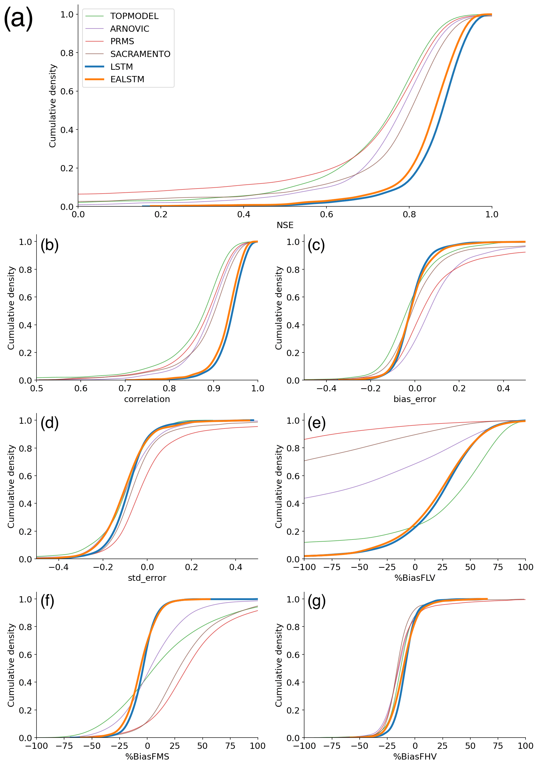
Figure 1 Cumulative distribution functions (CDFs) of station goodness-of-fit metric scores for each model. EA LSTM (orange) and the LSTM (blue), as well as the conceptual models: TOPMODEL (green), VIC (red), PRMS (purple) and SACRAMENTO (brown) (Lane et al., 2019). Panels indicate the distribution of stations: (a) NSE scores, (b) correlation scores, (c) bias error scores, (d) variability error scores, (e) low-flow bias scores, (f) mid-range of flow bias scores and (g) high-flow bias scores.

3.2 Spatial patterns of performance

The LSTM demonstrates competitive simulation of discharge across Great Britain (see the spatial patterns of various performance metrics in Fig. S6). The EA LSTM has very similar spatial patterns to the LSTM but shows a consistently worse performance than the LSTM across GB.

The benchmark conceptual models struggled when simulating discharge in catchments on the permeable bedrock in the south-east of England and the mountainous catchments in the north-east of Scotland (Lane et al., 2019). Performance metrics in the south-east were lower due to poor simulation of variance and correlation and in north-eastern Scotland due to poor simulation of the mean flow conditions (Lane et al., 2019). We suggest that these differences in performance are due to the low rainfall and chalk aquifer in the south-east of England and to the lack of snow modules incorporated into the conceptual models for north-eastern Scotland.

Interestingly, the LSTM simulates discharge less well in the south-east of England relative to LSTM performance elsewhere in GB, particularly in the summer months (Fig. 2). Performances for all seasons are worse in the south-east of England. This pattern is stronger in the summer months (JJA). The east–west gradient in model performances can be seen for all models, particularly in JJA. However, the range of errors is smaller for the LSTM-based models when compared with the conceptual models.

The LSTM shows an underestimate of the variability and a cluster of high bias scores in the south-east (Fig. S6). The LSTM both overestimated and underestimated mean flows in catchments in the south-east region, explaining the relative underperformance in the composite metric (NSE) for the LSTM relative to the rest of GB.

Spatial patterns in the biases for different sections of the flow duration curve show that only the LSTMs demonstrate a consistent underprediction of the midsection slope of the flow duration curve (%BiasFMS). A steep slope in the midsection of the flow duration curve reflects a watershed having a “flashy” response (Yilmaz et al., 2008), potentially due to low soil moisture capacity. Therefore, an underprediction of the midsection reflects an underestimation of the “flashiness” of the catchment. The LSTM %BiasFMS is largest for the south-east of England. The LSTM shows improved performance compared to the benchmark models across GB, including these underperforming regions, the south-east of England and north-eastern Scotland.

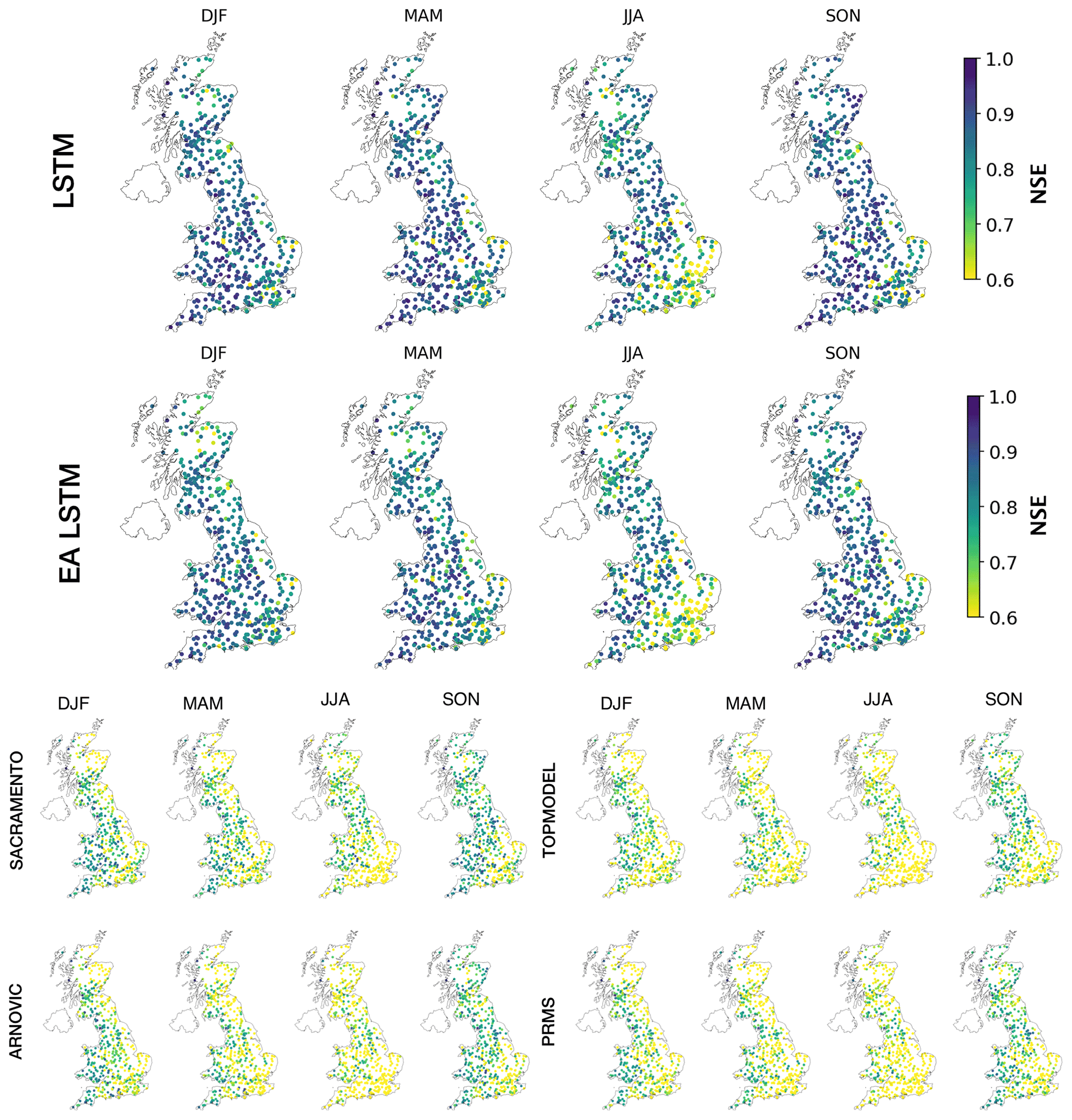
Figure 2 Seasonal NSE patterns for the two LSTM-based models (above) and the conceptual models (below). Each station in the evaluation data is shown as a point. The colour of the point reflects the NSE score. Brighter colours reflect lower NSE values, currently capped at a minimum of 0.7 NSE.

3.3 In what hydrological conditions do model performances differ?

Large sample studies allow us to detect catchment attributes that our models are or are not able to represent. In order to determine what the LSTM is capable of representing well, we perform two analyses. Firstly, we directly calculate the difference in NSE scores. Secondly, we correlate catchment attributes with model diagnostic scores.

The Δ_meanNSE is the mean difference between a reference model (LSTM) and the comparison model. The Δ_medianNSE is the median difference. The mean differences between the LSTM station NSE and the other models is smallest for the EA LSTM (Δ_meanNSE =0.02). This is unsurprising given the very similar architectures of the two models. The differences for the conceptual models range from TOPMODEL (Δ_meanNSE =0.15), ARNOVIC (Δ_meanNSE =0.17), SACRAMENTO (Δ_meanNSE =0.20) and PRMS (Δ_meanNSE =0.43). While the mean performances show large differences, due to the presence of poorly performing stations, the median differences are smaller for SACRAMENTO (Δ_medianNSE =0.07), ARNOVIC (Δ_medianNSE =0.09), PRMS (Δ_medianNSE =0.10) and TOPMODEL (Δ_medianNSE =0.10). Both summaries (median, mean) demonstrate that the LSTM offers a single model architecture that offers more accurate simulations than traditional hydrological models in a variety of hydrological conditions.

Spatially, the benchmark conceptual models struggled to produce good simulations in two geographical regions. These were in the south-east of England and north-east of Scotland. The performance improvement (ΔNSE) of the LSTM over the conceptual model was indeed largest in the south-east of England and north-eastern Scotland (see Fig. 3).

Figure 3 The performance improvement of the LSTM relative to the four conceptual models SACRAMENTO, ARNOVIC, TOPMODEL and PRMS. The difference in NSE is calculated by subtracting the conceptual model NSE from the LSTM NSE ($\mathrm{\Delta }\mathrm{NSE}={\mathrm{NSE}}_{\mathrm{LSTM}}-{\mathrm{NSE}}_{\mathrm{conceptual}}$). Each point represents a station, and the colour reflects the performance improvement (measured by NSE) of the LSTM compared with the conceptual models. Positive values reflect stations where the LSTM outperforms the conceptual models.

North-eastern Scotland is one of the most mountainous regions of GB. The Cairngorm National Park and the North Pennines are the only areas of GB where snow processes are consistently important, owing to catchments having a higher elevation. There are 36 catchments in the CAMELS-GB dataset with fraction of snow cover greater than 5 %, and 3 catchments are in the North Pennines; the other 33 catchments are in the Cairngorm National Park. The results in Fig. 3 show that the LSTM exhibits a large performance improvement in these catchments, since ΔNSE is high. This is most likely due to the cell state being able to represent longer-term stores and fluxes of water, therefore capturing the melting snow processes. The conceptual models lack a snow module and are therefore unable to capture snow melt or frozen ground processes, which are especially important in winter (DJF) and spring (MAM) (Lane et al., 2019). By contrast, what the LSTM performance shows is that data-driven models are able to flexibly incorporate snow processes in the catchments where they are required (NE Scotland) even when trained to produce one set of weights. This flexibility is an important asset of data-driven approaches, since these hydrological processes do not need to be specified prior to model training but can be learnt from the available data.

The south-east is a relatively dry area, with large chalk aquifers, contributing to a high baseflow index, and large urban and agricultural areas, contributing to a large anthropogenic signal in the hydrographs. Although the improvement in simulation accuracy compared to the conceptual models is large in the south-east, the pattern of raw LSTM NSE shows that the LSTM still underperforms in the south-east relative to elsewhere in GB. The seasonal patterns showed that the LSTMs performed worse in summer months, which is the drier period of the year. Consistent with this spatial pattern, the ratio of mean potential evapotranspiration to mean precipitation attribute (labelled “aridity” in the CAMELS-GB dataset; Coxon et al., 2020b) is negatively correlated with model performance for all models (Fig. 4), although the magnitude of this association is smaller for the LSTM-based models than the conceptual models.

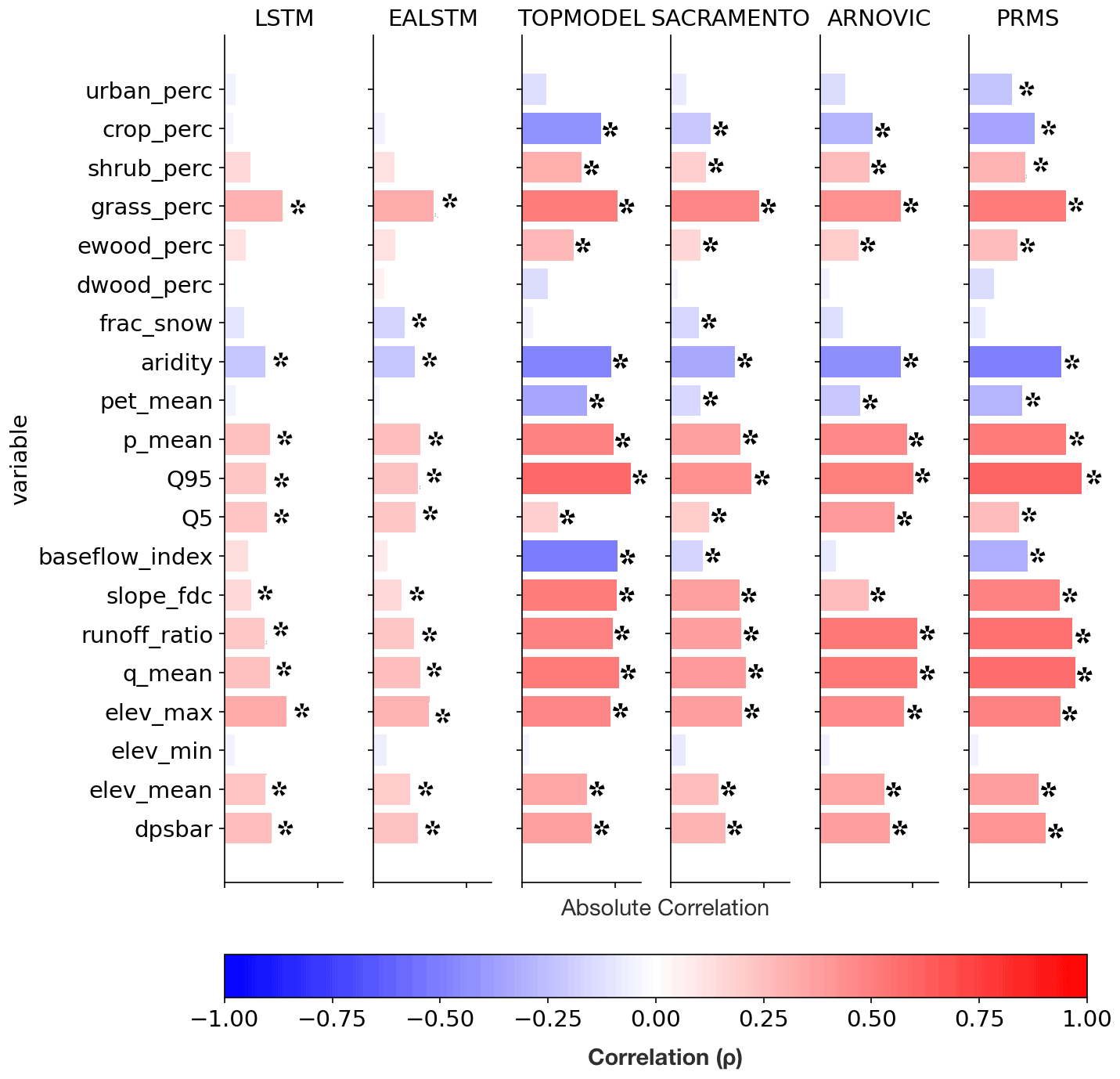
Figure 4 Static features (rows) and their Spearman’s rank correlation coefficient with model (columns) NSE scores. The positive correlations are in blue, and the negative correlations are in red. Pale bars show very low correlations. Symbol “*” indicates that the correlation is significant at the α=0.001 level. The first six features can be classified as land cover features. The next four features are climatic indices. The next six features are hydrologic attributes and the final four are topographic features. “dpsbar” refers to the mean drainage path slope and reflects the average steepness of a catchment.

We observe consistently poorer performance across all models, including the LSTMs, in drier hydrological conditions. This can be seen by the negative correlations between catchment P $/$ PET (aridity) and model NSE scores (Fig. 4).

The LSTM-based models show no significant correlation between baseflow index and model performances, in contrast with the other models. ARNOVIC also shows no significant correlation. ARNOVIC's improved performance can be attributed to the non-linear relationship in the upper storage, which means that the model will only produce very fast responses when that storage is very close to full (Lane et al., 2019).

3.3.1 The impact of water balance closure on simulation accuracy

One of the key hydrological conditions that hydrological models struggle with is the lack of closure of the catchment water balance. The conceptual models we test here explicitly maintain mass balance. They define the topographic surface water catchment as the surface over which water is conserved; i.e. the surface water catchment is not expected to leak nor should any water enter the catchment other than through measured precipitation. This will not then capture water losses or gains from undercatch, drifting snow, advection of fog, groundwater, or anthropogenic transfers into or out of the topographic catchment. Consequently, we would not expect the conceptual models to take account of catchments where the water balance (defined in the data) does not close. The LSTM, in contrast, is free to adjust to account for patterns in these anomalies. It is not yet possible to diagnose the origin of any such anomalies using the LSTM alone: they may arise from inter-catchment transfers (either through anthropogenic or groundwater processes) or data errors, among other reasons that the water balance might not be closed based on observations at the catchment scale. In spite of this, we expect that the LSTM will show improved performance in these catchments where there is no closure of the catchment water balance in the underlying dataset. Since we are calculating performance on out-of-sample time steps, if the LSTM performance is improved, we can infer that the LSTM-based model has learnt to correct these inconsistencies in a way which is consistent between training and evaluation data and is therefore adjusting the catchment water balance to better simulate the hydrograph.

We plot catchments on two dimensions (Fig. 5), their wetness index (P $/$ PE) and the runoff coefficient (Q $/$ P), to identify catchments where water is not conserved. Points above the horizontal line reflect catchments where the observed discharge is greater than the precipitation input to the catchment. This area of the graph represents catchments where the data have too little water to generate the observed runoff. Points below the curved line are where runoff deficits exceed total PET in a catchment. This area of the graph represents catchments where PET is not large enough to describe the water remaining after runoff is accounted for; i.e. the data have “excess” water (Fig. 5).

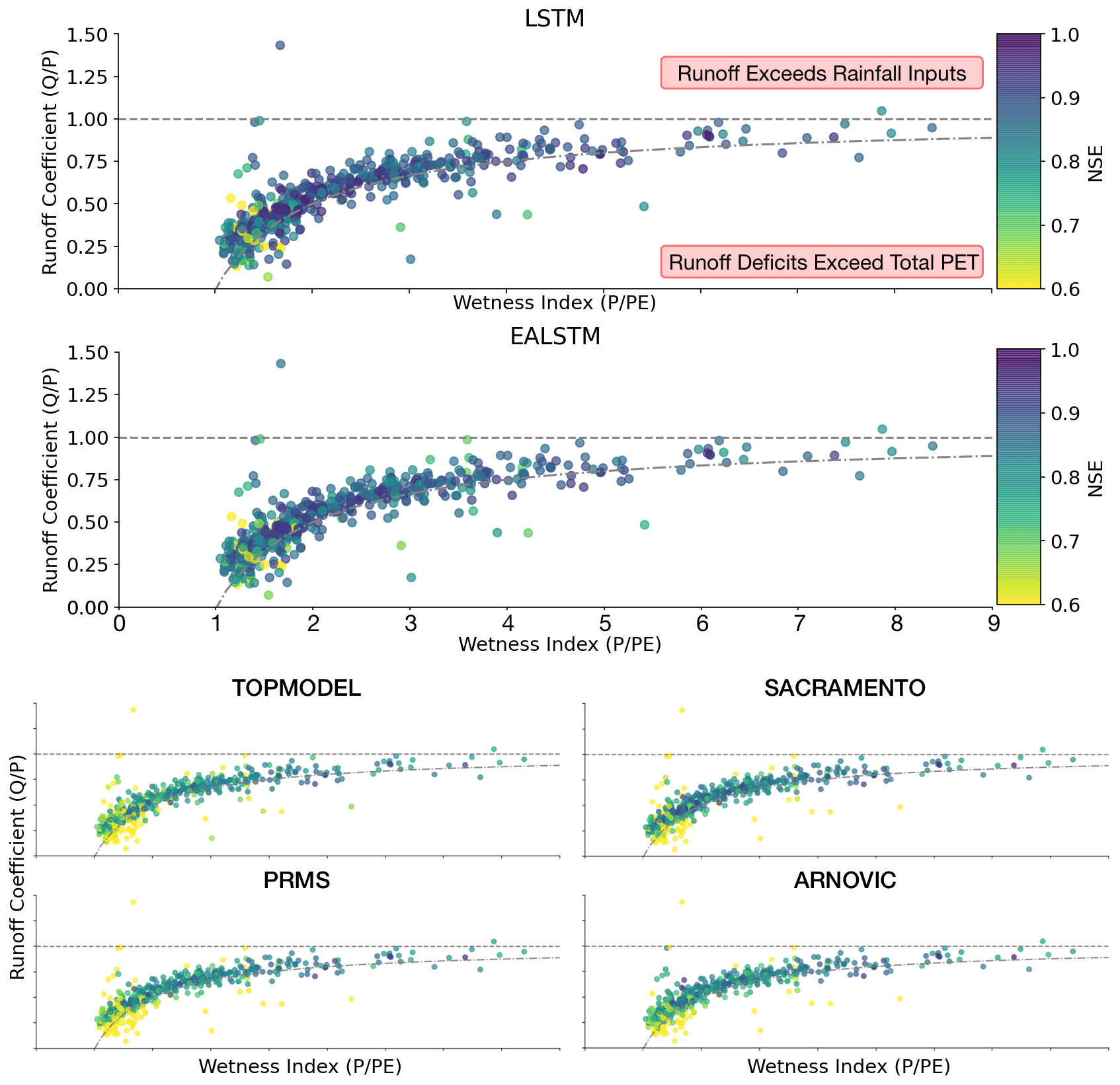
Figure 5 Scatter plot for the relationship between the wetness index, runoff coefficient and the model NSE score. Each point is a catchment, coloured by the NSE score ranging from 0.8 (lighter) to 1.0 (darker). Points above the horizontal line reflect catchments where the observed discharge is greater than the precipitation input to the catchment. Points below the curved line are where runoff deficits exceed total PET in a catchment; therefore, there is excess water in the data, since PET cannot explain the leftover water after accounting for runoff.

We tested whether the LSTM was better able to simulate discharge in catchments with excess water (i.e. the points below the curved lines in Fig. 5, which are then represented by the orange kernel density estimate in Fig. 6). As hypothesized, we find that the LSTM is more robust to these conditions and produces NSE scores that are comparable to the stations where the conceptual models perform best.

Interestingly, despite the performance improvement over the benchmark conceptual models, the LSTMs continue to produce a performance decline in catchments with an imbalanced water balance (Fig. 6). This suggests that the LSTM models still struggle with water-limited and energy-limited (low runoff coefficient and low wetness index) catchments. This could be because human management decisions that lead to abstractions are unpredictable without further dynamic inputs, such as timings of abstractions and effluent returns, or else that the underlying data do not contain sufficient geological information to describe the complex percolation and surface or subsurface connectivity pathways that cause a surface water catchment to leak.

Ultimately, the performance decline is less pronounced for the LSTM. The LSTM continues to produce simulations with NSE scores greater than 0.6. This suggests that there remains information in the data that the LSTM is capable of using to maintain accurate simulations in out-of-sample conditions.

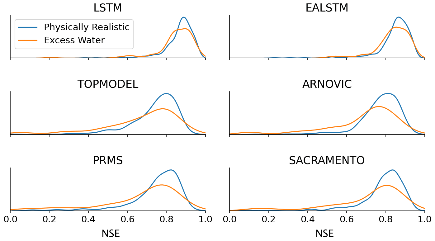
Figure 6 Comparing the NSE results for catchments that have excess water, where runoff deficits exceed total PET (orange), to those catchments that have physically realistic conditions (blue). The orange line shows the histograms for stations that fall below the curved line in the Budyko analysis above (the runoff deficit exceeds total PET; therefore there is excess water in the model). The blue line shows the histograms for those stations between the two dashed lines.

4 Discussion

This study benchmarks the performance of the LSTM using four commonly used conceptual models as a reference. The LSTM produced accurate simulations for a large number of catchments across Great Britain. The performance of the LSTM demonstrates that there is adequate information in the observational data to accurately simulate discharge behaviours across the various hydrological conditions found in Great Britain. The simulated time series and catchment error metrics can be found at https://doi.org/10.5281/zenodo.4555820.

In the discussion that follows we return to our three research questions. (i) How well do LSTM-based models simulate discharge in Great Britain? (ii) How do LSTM-based model performances compare with the conceptual models used as a benchmark? (iii) Can we extract information from the spatial and temporal patterns in diagnostic measures?

4.1 Inter-model performances

The LSTM-based models produce accurate simulations of discharge across GB, a temperate region. Two findings from this research confirm and extend the conclusions of previous work. First, the LSTM consistently outperforms the EA LSTM (Kratzert et al., 2019). Secondly, both LSTM-based models demonstrate improved simulation accuracy for discharge modelling compared with the conceptual models we use as benchmarks.

4.1.1 How well do LSTM-based models simulate discharge in Great Britain?

The EA LSTM is constrained to treat information that does not vary over time (catchment attributes) separately from information that varies over time (hydro-meteorological forcings). However, the constraint penalizes performance, which was also found by Kratzert et al. (2019). The EA LSTM, in contrast to LSTM, is forced to keep the input gate static through time. The input gate receives only information about catchment attributes. This means that no time-varying information is passed through the EA LSTM input gate. In contrast, the LSTM gates receive information from both time-varying meteorological inputs and static catchment attributes. The underperformance of the EA LSTM relative to the LSTM suggests that this regularization hurts performance in out-of-sample conditions.

It is worth noting that the LSTM and EA LSTM also differ in terms of practical computational requirements. The LSTM trains much faster than the EA LSTM. The LSTM will train 30 epochs in 1 h compared with 30 epochs in 10 h for the EA LSTM. This is due to the LSTM being an in-built PyTorch (v.1.7.1) function that makes use of CUDA-optimized code (for running the models on a GPU). In contrast, the EA LSTM relies on custom code without the CUDA-enabled optimizations.

4.1.2 How do the LSTM performances compare with the conceptual models used as a benchmark?

We have demonstrated that the LSTM is an effective model architecture for extracting information from hydro-meteorological data, providing a data-driven benchmark showing what is achievable given the information contained in available observation data from CAMELS-GB (Nearing et al., 2021). The LSTMs demonstrate better performance on out-of-sample times than in-sample performance from the benchmark conceptual models.

There are obvious challenges with direct comparison of LSTM performance against the benchmark developed by Lane et al. (2019). The first is that the LSTM is not constrained to maintain water mass balance, whereas the conceptual models discussed here are. Another challenge is that the method of optimization used for choosing parameters in the LSTM (stochastic gradient descent) is different to the random-sampling and NSE selection criteria used to select the “best” model parameters for the conceptual models. The sampling process used by Lane et al. (2019) is explicitly for estimating uncertainty as well as providing a reference of conceptual model performances. Another difference is that the LSTM diagnostic scores are calculated on out-of-sample predictions, compared with the in-sample predictions for the benchmark conceptual models.

Finally, the LSTM-based models are trained on all basins, with a single set of weights for the whole of GB. Therefore, these LSTM models are regional models that are able to reproduce behaviours across Great Britain. In contrast, most hydrological models perform best when calibrated on individual basins (Beven, 2006a). By contrast, LSTM-based models are most accurate when trained with as much data from as many catchments as possible (Gauch et al., 2021b). It is important to interpret the number of parameters for each model type in light of this fact.

The catchments where the comparative performance difference is small, i.e. where the conceptual models perform almost as well as the LSTM, reflect areas where the conceptual models capture the majority of the information from the data, and the conceptual model well represents the hydrological process. This is the case in western Scotland, north-western England and northern Wales, and north-eastern England (see Fig. S7). The benchmark results are valuable in providing a reference point for us to assess the value of LSTM-based approaches. We welcome future studies that use the LSTM simulations provided here and that further explore performance differences and the limitations of DL methods across GB.

4.1.3 Can we extract information from the spatial and temporal patterns in diagnostic measures?

The LSTM shows the largest performance improvement over the conceptual models in the north-west of Scotland and the south-east of England. The performance differences in north-western Scotland are very likely a result of the ability of the LSTM to learn a representation of snow processes from the input data, whereas the conceptual models were simulating these catchments without a snow module.

Despite the performance improvement over conceptual models in the south-east of England, the LSTM still struggles in the south-east relative to elsewhere in GB. The south-east is a relatively dry region compared to elsewhere in GB. It contains the highest proportion of catchments that fall below the dashed line in Fig. 5 and therefore stations where the surface water catchment is “leaky”. Furthermore, there are underlying chalk aquifers which provide water storage and lateral transfers. We outline three hypotheses for why the LSTM performance may be lower in the south-east compared with elsewhere in GB.

The first hypothesis is linked to the training of the LSTM-based models. The LSTM shows a performance decline in drier conditions (Fig. 4, see “aridity”). This confirms the findings of other DL studies in the USA, where the LSTM also struggled to reproduce hydrographs in drier conditions (Kratzert et al., 2019, 2018). Basins that have long periods of low flow contain little information, since changing meteorological inputs co-occurs with very little change in the target discharge. Therefore, the physical process relating meteorological inputs to river discharge can only be inferred from those catchments with varying discharge. There is some evidence for this hypothesis. NSE scores show positive correlations with increased discharge (at mean flow, Q5 and Q95), as well as increased NSE as rainfall increases (p_mean) (Fig. 4).

A related but separate hypothesis is that the use of NSE as an objective function fails to adequately weight performance in these low-flow regimes (the NSE was the objective function across both the conceptual models and the DL models).

A final hypothesis is that groundwater dynamics and human abstractions, which influence catchments in the south-east, are not well captured by the variables in CAMELS-GB. Hydrological processes are not simulated as effectively in leaky catchments compared to those catchments where the water balance can be closed with hydrometric data (Sect. 3.3.1), even using a very flexible and effective data-driven model that is not constrained to balance water (the LSTM). This suggests that the underlying data do not contain sufficient information to model the full range of processes that influence the hydrograph in these catchments, including groundwater and abstractions. The catchment-averaged information on soil texture (sand–silt–clay) provides a coarse proxy for catchment porosity. Furthermore, further data, such as groundwater time series, might be necessary to obtain more accurate discharge predictions. We suggest that different input datasets should be tested to try and improve LSTM performances, enabling the LSTM to more properly account for the complex percolation and infiltration dynamics in these catchments.

In terms of the seasonal patterns in LSTM performances and the worse performances in summer, the above hypotheses also apply, since the summer is the driest season in GB. Despite this, the LSTM-based models have been able to use the information in the available data to better model summer (JJA) discharge than the benchmark models. As in the data-based mechanistic modelling framework (Young, 2003), the next stage for hydrologists is to search for a mechanistic interpretation of the learnt model structure; also see Nearing et al. (2021). One possible mechanistic interpretation that warrants further exploration is the idea that the LSTM is capable of learning seasonally varying catchment “connectivity” (Bracken and Croke, 2007). In winter, when soils are saturated, there are a greater number of pathways for water to enter river channels, and connectivity is high. In summer, however, there is greater resistance to water flow, since water can be absorbed and stored in drier soils, as found in Swiss catchments by van Meerveld et al. (2019), and connectivity is lower. Connectivity information could be represented by the hidden state (h_t) or cell state vectors (C_t). The proposed impact of catchment connectivity on the performance improvement of the LSTM-based models is ultimately speculative, and future work will explore whether the LSTM has learnt to represent the concept of connectivity and seasonally variable flow pathways.

In contrast with the benchmark conceptual models, the LSTM-based model NSE scores have no negative correlation with crop cover percentage (Fig. 4). It is possible that the LSTM has effectively used the cropland cover variable to improve its internal representation of hydrology in those catchments with a strong agricultural signal. In order to test this hypothesis, one could perform an ablation study, removing input features and determining the impact on model performances. Alternatively, sensitivity analysis could be used to determine the relative contribution of the input features to the discharge prediction, thus revealing what input features are important for the model simulations. We intend to pursue this idea in upcoming papers.

Ultimately, compared with the benchmark models, the LSTM shows robustness to catchment conditions associated with poor conceptual model performance. Dry catchments, catchments with a strong agricultural signal, and summer discharges are all strongly correlated with worse conceptual model performances. In contrast, the LSTM has good performance on out-of-sample times in these same conditions. There is therefore information that the LSTM has learnt to generalize from the CAMELS-GB dataset that the conceptual models are not utilizing. The experiments we present here demonstrate conditions in which we can (and cannot) improve our traditional hydrological models given the availability of high-quality, large-sample datasets (Nearing et al., 2020; Beven, 2006b).

5 Conclusions

In this study we have benchmarked the performance of two LSTM-based models trained on 669 catchments across Great Britain. We have demonstrated that LSTM-based models trained on a large sample of catchment-averaged hydro-meteorological time series produce accurate simulations across GB. There is clearly information available in CAMELS-GB for modelling diverse hydrological conditions, and the LSTM performances should be interpreted as a competitive reference for what simulation performance is possible for out-of-sample (in time) conditions. We trained an ensemble of LSTM-based models to account for random initialization during the training process of these deep learning models, which also provides an estimate of prediction uncertainty (Sect. S4). The ensemble mean simulation produces median NSE scores of 0.88 (LSTM) and 0.86 (EA LSTM), with no catchments scoring NSE below 0. These results are consistent with the findings from Kratzert et al. (2018) in a different geographical context.

We have explored the spatial and temporal patterns in LSTM and EA LSTM performances, using the large sample of catchments to better understand the conditions in which the LSTM-based models perform well compared to themselves (LSTM in catchment A vs. LSTM in catchment B) and compared with traditional conceptual models. The results show that LSTM-based model performances are more robust to hydro-climatic conditions in the south-east of England, in more arid catchments and in catchments where the water balance does not close. This suggests that there is more information in large-sample datasets such as CAMELS-GB than is captured by hydrological theory as encoded in the benchmark conceptual models. Further work remains to determine what information has been learnt by these LSTM-based models, to use that information to improve hydrological theories and to feed them back, if possible, into further developments in conceptual and physically based models.

Relative to the LSTM-based model performances elsewhere in GB, the LSTM-based models continue to underperform in south-eastern England relative to elsewhere in GB. Considering the catchment conditions that are associated with this pattern, it is clear that all models struggle with drier conditions and catchments where the water balance does not close. It also seems possible that the training process fails to capture hydrological behaviours in drier catchments. There are a number of possible reasons. Firstly, changing meteorological conditions in dry catchments lead to little or no change in discharge (as would be the case in ephemeral streams). Alternatively, the LSTM architecture may not be capable of simulating both dry catchments and those with a higher runoff ratio using just a single set of weights. Finally, the data may not contain sufficient information to capture the percolation and connectivity dynamics that drive hydrological behaviour in catchments with significant groundwater processes. Further studies will examine the internal representation of hydrological processes in these catchments to better understand what the LSTM has or has not learnt about connectivity and groundwater processes.

This paper benchmarks LSTM performance across Great Britain using a new large-sample dataset, i.e. CAMELS-GB (Coxon et al., 2020b), providing a reference for future hydrological modelling efforts. Furthermore, this article outlines the hydrological conditions in which the LSTM-based models perform well and those conditions which are more difficult to model. We encourage future benchmarking studies to include LSTMs as a competitive model choice for simulating rainfall–runoff processes.