the Creative Commons Attribution 4.0 License.
the Creative Commons Attribution 4.0 License.
 | 12 Oct 2021
Numerical daemons of hydrological models are summoned by extreme precipitation
Peter T. La Follette
Adriaan J. Teuling
Nans Addor
Martyn Clark
Koen Jansen
Hydrological models are usually systems of nonlinear differential equations for which no analytical solutions exist and thus rely on numerical solutions. While some studies have investigated the relationship between numerical method choice and model error, the extent to which extreme precipitation such as that observed during hurricanes Harvey and Katrina impacts numerical error of hydrological models is still unknown. This knowledge is relevant in light of climate change, where many regions will likely experience more intense precipitation. In this experiment, a large number of hydrographs are generated with the modular modeling framework FUSE (Framework for Understanding Structural Errors), using eight numerical techniques across a variety of forcing data sets. All constructed models are conceptual and lumped. Multiple model structures, parameter sets, and initial conditions are incorporated for generality. The computational cost and numerical error associated with each hydrograph were recorded. Numerical error is assessed via root mean square error and normalized root mean square error. It was found that the root mean square error usually increases with precipitation intensity and decreases with event duration. Some numerical methods constrain errors much more effectively than others, sometimes by many orders of magnitude. Of the tested numerical methods, a second-order adaptive explicit method is found to be the most efficient because it has both a small numerical error and a low computational cost. A small literature review indicates that many popular modeling codes use numerical techniques that were suggested by this experiment to be suboptimal. We conclude that relatively large numerical errors may be common in current models, highlighting the need for robust numerical techniques, in particular in the face of increasing precipitation extremes.
- Article
(2204 KB) - Full-text XML
-
Supplement
(65 KB) - BibTeX
- EndNote


Computational hydrological models describe the movement and distribution of water within a region. They enjoy frequent use within and outside of academia, addressing a diversity of topics from the determination of catchment characteristics (Kirchner, 2009; Rempe and Dietrich, 2014; Wrede et al., 2015; Melsen et al., 2018), and assessing water supply security (Paton et al., 2013), to deciding which areas are in danger of flooding (Jasper et al., 2002; Madsen et al., 2014).
Hydrological models usually have state variables, which describe relevant physical quantities, and fluxes, which describe how the state variables change over time or space. For example, a state variable could be the amount of water in the unsaturated zone of a catchment, and fluxes interacting with that state variable could be evaporation, percolation to the saturated zone, discharge from the catchment, or precipitation, among others. Differential equations are used to describe the relationships between fluxes and state variables. These differential equations are often highly nonlinear, meaning that it is impossible to obtain their exact solutions. However, approximate solutions to these systems of differential equations are possible through a variety of numerical strategies. Therefore, hydrological models contain mathematical relationships between state variables and fluxes (as well as relationships between state variables themselves) that need to be solved numerically (approximately) rather than analytically (exactly).
While discharge predictions resulting from hydrological models are often reasonably accurate (Refsgaard and Knudsen, 1996; Refsgaard, 1997; Addor et al., 2011), they are always subject to error. Total hydrological model error can be decomposed in a few ways, i.e., observational, structural, and numerical, among others. Observational errors are differences between real and observed values caused by inaccurate measurements, and structural errors are differences between model results and observed quantities due to the conceptual simplification or misrepresentation of processes in a model compared to reality. Numerical errors are differences between the exact and approximate solutions to the set of equations composing the model that result from the choice of numerical method used to find an approximate solution (Higham, 2002). While many recent efforts in hydrology have advanced observational data quality (Wrede et al., 2015; Kittel et al., 2018) or structural representations of nature (Wrede et al., 2015; Melsen et al., 2018; Melsen and Guse, 2019; Prancevic and Kirchner, 2019; Dralle et al., 2018; Coxon et al., 2014), relatively few studies investigate the effects of numerical choices on model error. Notably, it has been demonstrated that numerical method choice has a large impact on hydrological modeling error (Clark and Kavetski, 2010; Kavetski and Clark, 2010). These papers test the ability of various numerical methods to approximate exact solutions and to predict real discharges, including fixed step and adaptive methods, implicit, explicit, and semi-implicit methods, and first- and second-order methods. Changing these options leads to differences in how fluxes are calculated, and it is shown that certain combinations of these qualities allow for a relatively accurate approximation of the exact solution of a hydrological model.
The numerical daemons papers (Clark and Kavetski, 2010; Kavetski and Clark, 2010) provide useful numerical conventions in observational contexts, mainly under general hydroclimatic conditions. As the climate changes and extreme precipitation events become more common (Trenberth, 2011; Meehl et al., 2005; Prein et al., 2017; Huang et al., 2020), one might expect numerical errors to become larger. It is simple to demonstrate that numerical errors could depend on precipitation extremeness, as in Fig. 1.
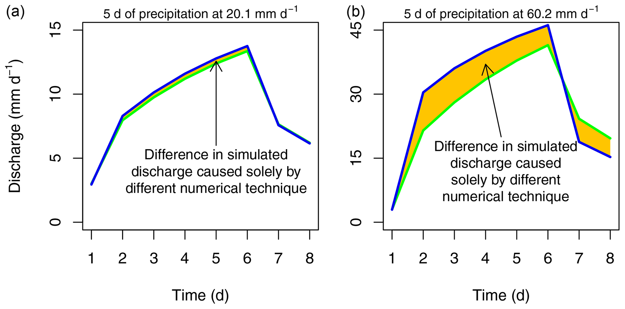
Figure 1Illustration of the impact of precipitation intensity on differences between discharge simulations from the same model but with two different numerical techniques. Discharge hydrographs are shown resulting from two different numerical methods, indicated by blue and green. These are the fixed step explicit Heun and adaptive implicit Heun methods, respectively, as discussed in Sect. 2. The only difference between the left and right plots is that the precipitation intensity is 3 times greater during days 2 through 6 for the right plot. With this figure, we do not suggest that any particular climate's precipitation will triple; this is merely used to demonstrate the relationship between precipitation intensity and potential numerical error.
This figure shows discharge hydrographs resulting from a model using two different numerical methods. The conditions yielding the left and right plots are identical in every way, except for the precipitation intensity used to simulate discharge, which is 3 times larger in the graph on the right. The only differences between the blue and green hydrographs are caused by choice of numerical method. Clearly, the two methods agree relatively poorly when higher intensity precipitation data are used; thus, there is a greater opportunity for a numerical method to provide an erroneous representation of the exact solution when precipitation is more intense. This is compatible with the findings that models can perform relatively poorly under relatively intense precipitation regimes (Weerts and El Serafy, 2006; Noh et al., 2014; Jasper et al., 2002) where it is possible that numerical error contributes to total modeling error. Furthermore, one might intuitively expect greater numerical errors for more extreme precipitation. The amount of water precipitated by a more extreme storm may be comparable to the total storage of a model, whereas this is not the case for milder storms. Given a sufficiently large time step or large enough flux, fixed step numerical solvers are not equipped to handle large precipitation events. In essence, it is known that numerical error can contribute significantly to total modeling error, and it is known that total modeling errors can increase with increasing precipitation extremeness, but it is currently not known how changing precipitation extremeness (intensity or duration) will impact the numerical error associated with a model.
In this paper, the same eight numerical methods as in Clark and Kavetski (2010) and Kavetski and Clark (2010) are studied (see Sect. 2 for descriptions of these methods). We aim to determine which qualities of these numerical methods contribute to numerical error as precipitation is varied from mild to extreme. To this end, the numerical error associated with each method is assessed over a broad range of precipitation intensities, ranging from mild to more intense than historically observed, for various event durations.
In order to thoroughly investigate the relationship between numerical error and precipitation extremeness for each numerical technique, testing must occur under a variety of conditions. Numerical error could depend on model structure (i.e., the specific relationship between state variables and fluxes, as well as choice of which state variables to include), physical setting (given by a specific combination of model parameters), and antecedent state variable values. This dependence is due to the fact that each of these will affect the set of differential equations composing a model. In order to systematically test these different conditions, a modular modeling framework (MMF) is required. Modular modeling frameworks are tools that are able to rapidly create hydrological models with various processes or structures included, varying numerical schemes (with some MMFs), and other options related to model setup or input. This allows a comparison of model results as these settings are systematically altered. The Framework for Understanding Structural Errors (FUSE) is the MMF selected for this experiment.
We are also interested in the change in efficiency of numerical techniques with respect to precipitation extremeness, where efficiency involves both the numerical error associated with a method and its computational expense. Therefore, trends in computational expense with changing precipitation are also assessed.
It is possible that many existing hydrological modeling codes use numerical methods that yield large numerical errors. In order to gain insight into how often relatively erroneous numerical methods might be employed, a small literature review is conducted on 12 popular modeling codes, determining the numerical options available in each. When the numerical techniques used by the reviewed codes are placed in the context of this study, an estimate of the potential magnitude of numerical errors arising from these codes is obtained.
In summary, we use an MMF to study the numerical error and computational expenses associated with different numerical techniques as precipitation varies from mild to extreme. This is carried out under a variety of initial conditions, parameter sets, and model structures for further generality. Trends in error and efficiency are analyzed. Then, a literature review suggests the prevalence of potential numerical errors in popular modeling codes. Finally, we present a discussion of the key findings and their practical implications for modeling, where we hypothesize that numerical errors can be reduced in practice via a careful selection of the numerical method.
A hydrological model is usually composed of a system of differential equations relating to state variables and fluxes. These equations are usually highly nonlinear, which means that they cannot be solved in closed form (though this is not always the case; see Coxon et al., 2019). Thus, a numerical approximation must be used. In this section, a description of the numerical techniques studied in this paper is given, together with a justification for the selection of these specific methods. The reader might choose to skip this section if familiar with numerical methods for approximating solutions of systems of differential equations.
In this experiment, each numerical technique is used to solve a system of coupled ordinary differential equations, where the equations are coupled because the flux from each state variable generally depends on multiple state variables. For example, the net flux from the saturated zone could be a function of the amount of water in the saturated zone and the amount of water in the unsaturated zone. These systems can be solved in two ways: via sequential solving (or operator splitting), where the equations are solved (and the state variables are updated) in some predetermined order, or via simultaneous solving, where all equations are solved at once (which requires a space-state formulation of the equations which compose a model). Sequential solvers are able to use different numerical methods for individual fluxes, which in some fields is desirable (for example, Glowinski et al., 2017 state that “splitting of diffusion terms and convection terms in a convection–diffusion partial differential equation” allows for a faster solution of the differential equation). However, when using sequential solvers, the model output may depend on the sequence in which state variables are solved, which is undesirable when comparing different model structures (Clark and Kavetski, 2010; Glowinski et al., 2017). Using the simultaneous method, N equations will be solved at the same time with the same numerical technique, where N is the total number of state variables, so that n=1, …, N in the equations of this section.
The simplest numerical method studied in this paper is the fixed step explicit Euler method (credited to Leonhard Euler). This method works by evaluating the flux for a state variable at the start of a time step, then adding this flux to the state variable at the beginning of the time step to generate the value for the state variable at the end of the time step. An illustrated example is given in Fig. 2a. Symbolically, the method is as follows:
where Δt is the time step, Sn is a state variable, fn is the time derivative, or net flux, of Sn at time t and is a function of S and t, and S is a vector of all relevant state variables for computing fn, determined by the model structure. The flux f is indicated to be a function of S and t because fluxes generally depend on both (for example, net flux to the unsaturated zone depends on precipitation, which is a function of time, and the amount of water in the unsaturated zone, which is a state variable). O(Δt) indicates that the truncation error – or the difference between this numerical approximation and an exact solution to the differential equation – is proportional to the size of the time step to the first power. This can be shown by equating the right-hand side of Eq. (2) to a Taylor series expansion of the left-hand side of Eq. (2), yielding error terms where the lowest order in Δt is 1. Thus, this method is first-order accurate. The method is known as fixed step because the time step can only be one value (in this experiment, all fixed steps are daily) and explicit because it calculates the flux using state variables that are already known (Süli and Mayers, 2003).
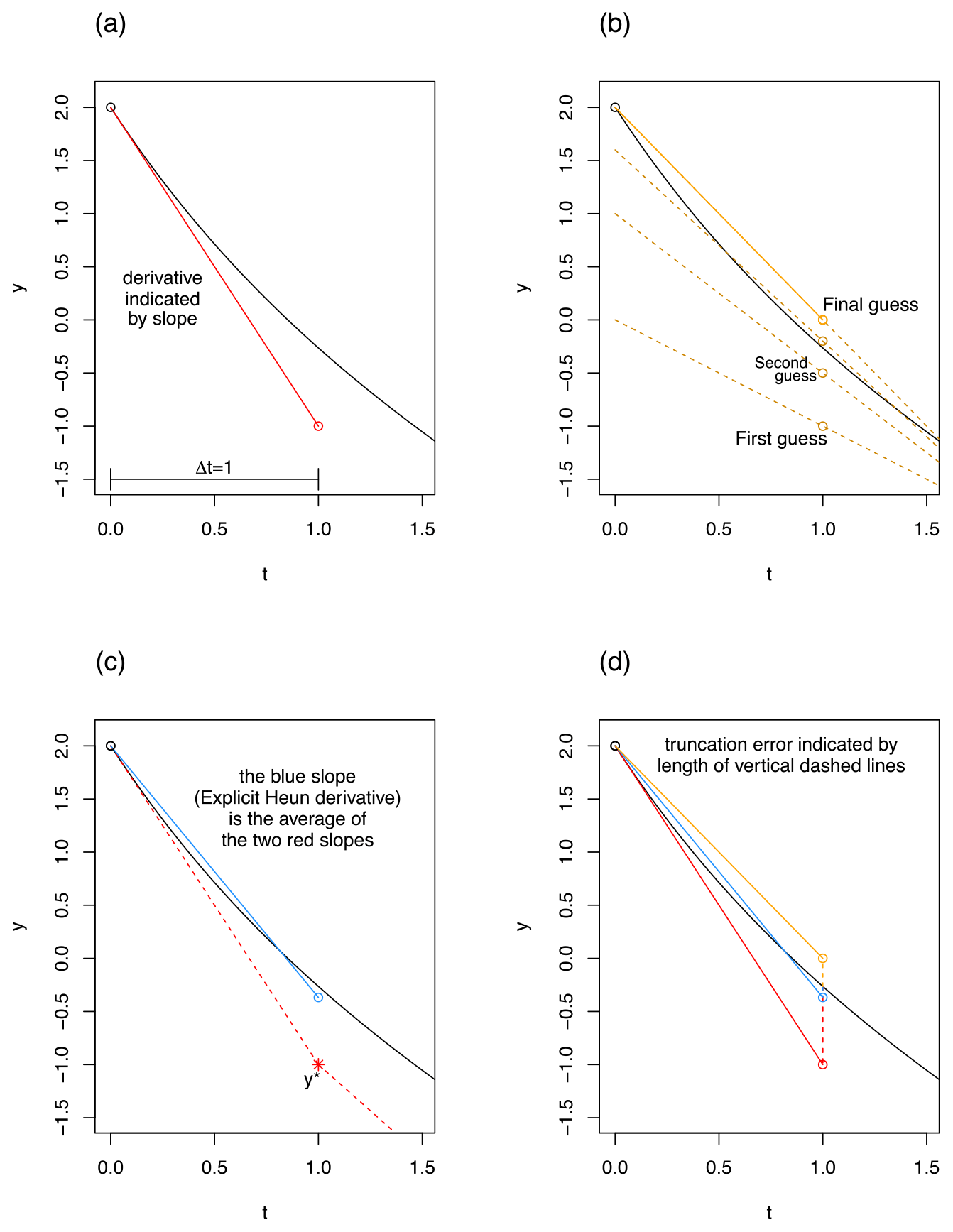
Figure 2Examples illustrating a single step of explicit Euler (a), implicit Euler (b), explicit Heun (c), and a comparison of all three (d). A single differential equation rather than a system is solved, given by , y(x(0))=2, where x(t)=t for simplicity. The black curve is the exact solution to this linear differential equation. Each approximation method uses a time step of 1 in these examples.
The fixed step implicit Euler method is similar to its explicit counterpart in that it is first-order accurate and has a fixed time step. It is different in that the derivative at the end of the time step, rather than the start of the time step, is used to calculate the state variable at the end of the time step. However, the derivative of a state variable is generally a function of the state variables, which are initially unknown for the end of the time step. So, the implicit Euler method must iteratively solve a system composed of equations in the style of Eq. (4) by searching for the values of S(t+Δt) which yield a derivative that matches Sn(t). In the graphical example of Fig. 2b, the value for y at the end of the time step is first approximated with an explicit Euler calculation, and then the method checks if the derivative there leads back to the value at the beginning of the time step within a given mass balance error tolerance (the mass balance error tolerance and monitoring methods are not studied in this paper). If not, this process is repeated with a new guess for Sn(t+Δt) until the derivative at the end of the time step leads back to the value of y at the beginning of the time step or graphically until the dotted orange line leads back to the value of y at t=0. Symbolically, the method is given by the following:
where fn is now the derivative of Sn at time t+Δt. The iterations required by fixed step implicit methods can make them more computationally expensive than their explicit counterparts. However, a property of implicit methods is that they are unconditionally stable (Jameson and Turkel, 1981) and can, in some situations, be more accurate than explicit methods.
The fixed step semi-implicit Euler method works by first performing an explicit Euler calculation, followed by a single correction in the style of implicit Euler. Visually, this would yield a result at the second guess value in Fig. 2b, and mathematically, this is achieved by a single iteration of Eq. (4) after the initial estimate of Sn(t+Δt). This method then theoretically has a computational expense usually somewhere between the fixed step implicit and explicit Euler methods and is first-order accurate. It is typically able to constrain instabilities (Kavetski et al., 2002).
The fixed step explicit Heun method (credited to Karl Heun) works by first explicitly calculating the derivative at the start of a time step (in exactly the same style as fixed step explicit Euler), then explicitly calculating the derivative at the end of the time step using the initial explicit Euler prediction, averaging the derivatives from the start and end of the time step, and then using this corrected average derivative in order to make a final prediction of the state variable value at the end of the time step. In Fig. 2c, the blue slope, or the explicit Heun derivative, is simply the average of both dotted red slopes, where the dotted red slope on the right is calculated using the initial explicit Euler result y* at t=1, and the dotted red slope on the left is the same slope as in Fig. 2a. Symbolically, the method is as follows:
where is the initial explicit Euler prediction of the state variables. This is a second-order method; its truncation error is proportional to Δt2, meaning that as Δt approaches 0, the truncation error approaches 0 faster than it would with first-order numerical methods.
The final tested fixed step method is the fixed step implicit Heun method, which is also second order. This method is commonly known as the implicit trapezoidal or trapezium method (Süli and Mayers, 2003). It is called the implicit Heun method in this paper due to the fact that it is an implicit analog of the explicit Heun method and for consistency with Clark and Kavetski (2010). The two Heun methods are similar in that they both use the explicit Euler prediction at the beginning of the time step, but the derivative is calculated implicitly in the implicit Heun method, incorporating both the known value of the state variables at time t and the initially unknown value of the state variables at time t+Δt. Symbolically, the method is as follows:
where Eq. (8) must be solved iteratively. Graphically, this will appear somewhat similar in method to Fig. 2b.
While so far only fixed step methods have been discussed, this paper also tests adaptive methods, which are able to adapt their step sizes based on various criteria. Adaptive methods can reduce numerical error, due to the fact that a reduced step size will reduce the truncation error. They can also reduce computational expense because a small step size is not always necessary for high numerical accuracy (Press and Teukolsky, 1992). This paper examines the following three adaptive methods: the adaptive semi-implicit Euler method, the adaptive explicit Heun method, and the adaptive implicit Heun method, which are all adaptive analogs of their fixed step counterparts. The adaptive semi-implicit Euler method adapts its step size by calculating the error e or the difference between its explicit Euler component and its final value. Specifically, after computing Sn(t+Δt), in the following, it checks whether:
where τr is the relative error tolerance (unitless), and τa is the absolute error tolerance; respectively, these default to 0.01 and 0.01 mm. Both e and Sn have units of millimeters. Each state variable must satisfy this threshold. If the step size is accepted, then Sn(t+Δt) is taken as the state variable for the end of the time step, and the step size is adjusted according to Appendix B in Clark and Kavetski (2010). If the step size is rejected, then it is reduced incrementally until convergence criteria are satisfied, which is also detailed in Appendix B of Clark and Kavetski (2010). The adaptive implicit and explicit Heun methods make the same comparison, although they do calculate e based on differences between a first-order component and the second-order prediction at the end of the time step rather than two first-order predictions as in the case of the adaptive semi-implicit Euler method (Clark and Kavetski, 2010). In all of these adaptive methods, various precalculated components are compared, so additional calculations are not needed for the sake of error control. Therefore these are embedded error control methods (Press and Teukolsky, 1992).
In total, eight distinct numerical methods are employed in this experiment. These broadly represent popular choices in hydrologic models (Clark and Kavetski, 2010); this is further tentatively supported by the results of the literature review (see Sect. 4.7), where none of the numerical techniques used by the surveyed modeling codes were significantly different from those available in FUSE. Nonetheless, here a few other choices in numerical methods are briefly described. Midpoint methods are similar to Heun methods in that they are second order (Süli and Mayers, 2003). The difference is that midpoint methods calculate an intermediate flux in the middle of the specified time step and then average this result with another preliminary flux calculated at the end of the time step in order to produce a final flux for the end of the time step, whereas Heun methods perform the same strategy on subsequent time steps (rather than subdividing a single time step). Higher order Runge–Kutta methods (credited to Carl Runge and Wilhelm Kutta) are also promising choices to numerically solve systems of differential equations; these methods take further terms in the Taylor expansion that is used to approximate the exact solution of a system of differential equations. They therefore have numerical errors which are proportional to the time step raised to the order of the method (e.g., a fifth-order method, as in Schoups et al., 2010). Finally, note that the models in this experiment are lumped rather than spatially distributed, and therefore, the backward Euler method, which is directly analogous to the implicit Euler method, is not considered.
This study aims to examine the relationship between precipitation extremeness and numerical error for a variety of numerical methods implemented in hydrological models. This section describes the conditions under which models are run, the methods by which numerical error and computational expense are assessed, and the conditions of the literature review by which the approximate magnitudes of errors resulting from popular modeling codes are assessed.
3.1 Modular modeling frameworks (MMFs) and the framework For Understanding Structural Errors (FUSE)
Modular modeling frameworks are fairly new tools in hydrology. These are pieces of code or software that are able to rapidly create hydrological models with various processes or structures included, varying numerical schemes (with some MMFs), and other options related to model setup or input. This allows for the controlled comparison of models, enabling studies on model structure, model uncertainty, and a wealth of other topics. In this case, an MMF offers the opportunity to study the change in numerical error resulting from the instantaneous (unrouted) discharge hydrograph as the dimensions of model structure, numerical method, parameters, initial conditions, and forcing data are systematically altered. This allows us to test for generality concerning the relation between numerical error and precipitation extremeness over a large dimensional space, as well as account for interactions among these dimensions.
The Framework for Understanding Structural Errors (FUSE) was selected for this experiment. To our best knowledge, this is the only MMF that allows for implicit and explicit numerical methods of higher order than 1. Note that the update to FUSE allowing for higher-order numerical techniques was introduced by Clark and Kavetski (2010), after FUSE's initial development (Clark et al., 2008).
The five different FUSE members, or five different model structures, are used to generate all hydrographs. Different combinations of state variables and fluxes are used in each. These include FUSE 070, 536, 550, 092, and 330, which are taken directly from Clark and Kavetski (2010) and are from a list of “models broadly representative of the wide spectrum of conceptual hydrological models used in research and practice”. All of these models are lumped rather than distributed. The FUSE snow module is always off in this experiment.
The model runs are generated across 20 parameter sets. This makes the results more generalizable, simulating hydrograph behavior in different physical settings. The parameter sets are generated via a Latin hypercube (LH) method, ensuring they cover as large a region of the parameter space as possible. The LH technique is used on the total set of parameters used across all models; each model, having a different structure, does not require the full set of LH-optimized parameters. In order to determine whether a sufficient number of parameter sets was used, hydrographs resulting from both 20 and 80 parameter sets are separately generated and compared.
3.2 Synthetic forcing data
In order to determine the change in model numerical error as precipitation varies from mild to extreme, a clearer idea of what constitutes extreme precipitation is required. Here, extreme precipitation is some combination of intense and long-lasting precipitation. In order to test the effect of both changing precipitation intensity and duration on numerical error, precipitation data sets are synthetically generated along the intensity, duration, and frequency (IDF) curves shown in Fig. 3. All points in Fig. 3 are World Meteorological Organization world records (World Meteorological Organization, 1994) in total precipitation for a given duration. We generate six IDF curves, representing interpolations between the world record events, scaled by factors of 0.01, 0.025, 0.075, 0.25, 1, and 1.2. These factors logarithmically span a large range of rainfall intensities, ranging from mild to larger than historically observed. The inclusion of precipitation events that are more intense than have been historically observed is due to the projected increase in wet day precipitation intensity under emission scenario SRES (Special Report on Emissions Scenarios) A2; for many regions, this exceeds 20 % when comparing the simulated periods 2081–2100 and 1980–1999 (Seneviratne et al., 2017). Synthetic precipitation data were generated along these interpolations for the following three different event durations: 5, 10, and 20 d. These are selected with the motivation that flood modeling for larger catchments is often done for precipitation events at these timescales (Jasper et al., 2002; Weerts and El Serafy, 2006). Thus, in total, 18 synthetic precipitation data sets were generated. The shape of the rainfall signals used in the majority of the analysis is flat, such that each day has the same precipitation intensity for a given event, though the effect of using precipitation data based on real events is briefly discussed. Total accumulated precipitation per event ranges between 40.1 mm (for the 5 d event with a daily intensity of 1 % of the average intensity of the interpolated 5 d historical maximum) and 9787.2 mm (for the 20 d event with a daily intensity of 120 % of the average intensity of the interpolated 20 d historical maximum).
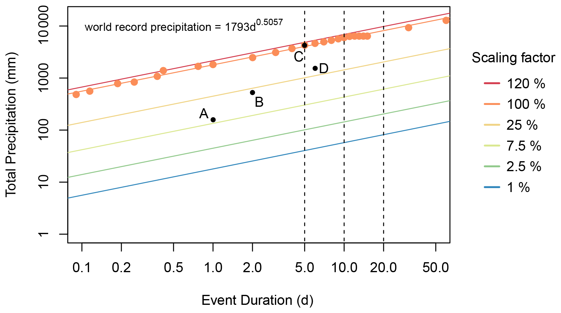
Figure 3Synthetic IDF (intensity, duration, and frequency) curves along which synthetic forcing data were generated, where the vertical black lines show the precipitation event durations used. The IDF curves are interpolated between world record events for given durations, scaled by 6 different factors, ranging from 0.01 to 1.2, indicated by color. The precipitation world records are World Meteorological Organization data (World Meteorological Organization, 1994) and are indicated by orange points. The power function giving the best fit for the world records is shown. Black points are real events which are described here in order to give further context for the IDF curves. (a) The largest precipitation ever recorded in the Netherlands in a 24 h period (Brauer et al., 2011). (b) An atmospheric river event in Sonoma County, California, USA, in late February 2019 (NOAA, 2019; Ralph et al., 2020). (c) Cyclone Hyacinthe (World Meteorological Organization, 1994). (d) Hurricane Harvey near Nederland, Texas, USA (Blake and Zelinsky, 2018).
It is also important to determine to what extent results depend on initial conditions. To this end, the forcing data are preceded by a 500 d spin-up period with one of three constant precipitation intensities, i.e., 2.5, 5, or 10 mm d−1. Each spin-up intensity is used with each of the above-described precipitation events. The goal of using these three intensities is not necessarily to simulate initial conditions which are characteristic of three distinct climatologies but rather to establish a broad range of initial conditions in terms of percent of maximum storage. Because we incorporate a broad variety of model structures and parameter sets, the total storage in the model at end of the spin-up period spans a variety of values, ranging from nearly empty (less than 1 % full) to approximately 70 % full. From least to most intense spin-up periods, median storages expressed as a percent of maximum storages at the end of the spin-up period are 21 %, 25 %, and 28 %, respectively. Comparing results from three different spin-up precipitation intensities allows for a systematic method by which to investigate initial conditions and their effect on the relative numerical errors of various numerical methods.
The synthetic forcing data sets are completed with potential evapotranspiration (ET) and temperature data. For all forcing data sets, constant potential ET values of 2 mm d−1 and temperatures of 10 ∘C are used. In most cases, the ET flux is small relative to the precipitation flux.
3.3 Method for determination of numerical error
For a fixed model structure (out of five), initial condition (out of three levels), parameter set (out of 20), and forcing data set (out of 18), there are nine instantaneous discharge hydrograph runs, corresponding to the eight tested numerical methods and the benchmark method. The benchmark method is the near-exact solution against which all other methods are compared. It is generated with the most sophisticated numerical technique available in FUSE, adaptive implicit Heun, with error tolerances 1000 times smaller than the defaults (; mm for the benchmark). A desirable property of the benchmark is that it yields approximate solutions that are much closer to the exact solutions than those resulting from any other method. To ensure this, the hydrograph resulting from the benchmark method, but with 10 times larger error tolerances, was compared to the discharge hydrographs from all other methods. It was found that the larger tolerance benchmark had lower error (when compared to the real benchmark) than any other method more than 99 % of the time.
The error for any tested run is determined by calculating the root mean square error (RMSE; millimeters per day, hereafter mm d−1) and normalized root mean square error (NRMSE; percent) with respect to the benchmark run. The RMSE is given by the following:
where T is the total time evaluated in days, is the near-exact discharge resulting from the benchmark method at time t, and qt is the discharge resulting from the numerical method being assessed at time t. The NRMSE is simply the RMSE normalized by the mean discharge of the associated benchmark run and then multiplied by 100 to become a percent. The time T for which the error is evaluated is 7 d for 5 d precipitation events, 14 d for 10 d precipitation events, and 28 d for 20 d precipitation events, always beginning on the first day of rainfall after the spin-up period. This is a somewhat arbitrary albeit valid period on which to evaluate hydrograph performance; it captures all or part of the rising limb, the crest segment, and the falling limb. Figure 4 shows example discharge hydrographs resulting from the fixed step explicit Heun method and the benchmark method. The total number of times the system of differential equations composing a model must be solved, or, alternatively, the number of system flux evaluations, is also recorded and represents the computational expense of generating the hydrograph.
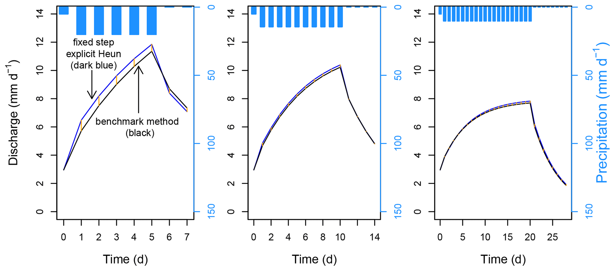
Figure 4Example hyetographs and discharge hydrographs, including results from the fixed step explicit Heun method and the benchmark method for 5, 10, and 20 d precipitation events. The vertical orange lines are the differences between the two hydrographs and represent the numerical error. From the shortest to the longest duration, the RMSEs are 0.55, 0.14, and 0.10 mm d−1. The precipitation forcing data come from the IDF curve scaled at 2.5 % of the historical maxima interpolation. These hydrographs all result from the same structure (FUSE 092), the same parameter set, and the same spin-up precipitation intensity (5 mm d−1). The last day of the spin-up period is shown.
RMSE and NRMSE are both included in this experiment because they show errors in two different yet valid ways, namely in the original units of the discharge and as a relative measure of the near-exact discharge, respectively. RMSE is useful in that its units (mm d−1) are easy to interpret, directly showing the numerical error in the daily discharge, while the benefit of NRMSE is that it provides context for the error. These definitions of error are purely numerical and, therefore, differ from fidelity as described in Clark and Kavetski (2010), which further incorporates real discharge observations.
3.4 Literature review
A small literature review determining available numerical strategies was conducted on 12 hydrological modeling codes. This included seven off-the-shelf models, which are the objects of study in Addor and Melsen (2019), and five popular MMFs. The reviewed modeling codes are shown in Appendix A. Information is gathered on whether recently updated versions of each modeling code are capable of sequential or simultaneous solving, available orders of numerical solver, the implicit or explicit (or other) nature of the numerical solver, and whether or not adaptive substepping is available. When solvers were found to have the option of simultaneous solving, all available numerical options were recorded. When solvers were found to only have sequential options – allowing for different numerical options per individual flux – the modeling code is considered to be restricted to the least sophisticated method specified among the fluxes encountered (specifically, we consider explicit methods to be less sophisticated than implicit methods, fixed step less sophisticated than adaptive, and lower order less sophisticated than higher order). This reflects our assumption that a numerically erroneous component of the model will produce errors which propagate to other components of the model; in other words, numerical accuracy is only as good as the most erroneous part of a model. This review has the objective of approximately placing other models or MMFs in the context of this experiment, which sheds light on what kinds of numerical errors might be expected as a result of using popular modeling codes.
We restrict the sampled models to those examined by Addor and Melsen (2019) for two reasons. First, Addor and Melsen (2019) chose these models based on their popularity rather than their numerical techniques. In this way, we do not cherry-pick models which either support or refute the premise that sophisticated numerical methods are common in current hydrologic models. Second, we limit the number of reviewed modeling codes because compiling a list of all current hydrologic models and their used numerical methods would provide a more accurate description of which numerical methods are widely used but represents a much larger project.
4.1 Numerical error and precipitation intensity for 5 d events
Figure 5 details the evolution of numerical errors for the tested numerical techniques for 5 d events of increasing precipitation intensity, for 20 parameter sets, all model structures, and all initial conditions. It is immediately apparent that, for all methods, median RMSE increases with increasing precipitation intensity, and second-order adaptive methods usually outperform fixed step methods (in some cases by a few orders of magnitude). The following two paragraphs explore trends in RMSE, shown in the top panel of Fig. 5, from left to right.

Figure 5Box plots showing the errors (RMSE shown in a and NRMSE shown in b) associated with associated with each numerical technique for 5 d precipitation events of increasing intensity, where the intensity is represented as a percentage of the interpolated world record 5 d event intensity. The solid black line in each box is the median error, the boxes extend to the 25 % and 75 % quantiles, and the whiskers extend to extreme values. All adaptive methods use the FUSE default error tolerances. Heun methods are second order, whereas Euler methods are first order. The model runs represented in this figure are generated across 20 parameter sets, five model structures, and three spin-up conditions.
For lower precipitation intensities, adaptive Heun methods usually outperform the other methods. The adaptive semi-implicit Euler method yielded more error than the other adaptive methods, putting this method on par with the second-order fixed step methods. The relatively low performance of adaptive semi-implicit Euler is likely due to the fact that the Heun methods adapt their step sizes based on comparisons between first- and second-order results, while the semi-implicit method adapts its step size based on a comparison between two first-order results. Here, all adaptive methods use the same default error tolerances, where the effects of changing these will be discussed later. Among fixed step methods, for lower precipitation intensities, first-order methods (the Euler methods) are on average outperformed by second-order methods (the Heun methods). Apparently, the extra flux evaluations required by second-order methods are able to reduce error in these low intensity cases.
As precipitation intensity increases, it is clear that adaptive methods outperform fixed step methods, where the adaptive semi-implicit Euler method begins to yield lower error than fixed step methods. For fixed step methods with higher precipitation intensity, it is no longer the case that second-order methods outperform first-order methods. Instead, implicit or semi-implicit methods outperform explicit methods; the fixed step explicit methods yield median errors above 70 mm d−1 for the two highest precipitation intensities. This indicates that instabilities contribute more significantly to numerical error as precipitation intensity increases, as implicit methods are unconditionally stable (Jameson and Turkel, 1981), and the semi-implicit method constrains instabilities more readily than the explicit methods (Kavetski et al., 2002). Furthermore, because fixed step explicit Heun clearly outperforms explicit Euler for low precipitation intensities but not for high precipitation intensities, and because fixed step implicit Heun and implicit Euler have this same property, we can conclude that higher-order truncation error is more sensitive to increasing precipitation intensity than first-order truncation error at the daily time step. This suggests that simply selecting an arbitrarily higher-order fixed step method will not always constrain error – and in some cases, it might make the error worse. Evidently, adaptive methods are most suitable for constraining numerical errors.
In the bottom panel of Fig. 5, the NRMSE is shown. All of the above-identified trends can be found here as well, except that the median error always increases with increasing precipitation intensity. With many (especially adaptive) methods, NRMSE decreases with increasing precipitation intensity. This is due to the fact that RMSE might usually increase, but not as fast as the discharge by which the RMSE is normalized. When this analysis was repeated with Kling–Gupta efficiency (Gupta et al., 2009), Nash–Sutcliffe efficiency (Nash and Sutcliffe, 1970), and normalized error in maximum discharge, similar trends in performance and precipitation intensity were obtained when compared to NRMSE.
To put the errors introduced by numerics into perspective, we compare it to other sources of error in hydrological modeling. Uncertainty in discharge measurements depends on the employed method, e.g., whether the observation is based on a rating curve or acoustic Doppler current profiler (ADCP; McMillan et al., 2017). Using a rating curve, Westerberg et al. (2011) observed for a specific case 20 % error for medium and high flows, due to nonstationarity of the channel, and McMillan et al. (2012) estimate discharge measurement uncertainty for medium to high flows even up to 40 %. Estimating the error in precipitation observations is more challenging because it not only depends on the measurement device but also on the spatial representativeness of the measurement. Wood et al. (2000) estimate a 50 % error in rainfall observations when comparing radar and tipping buckets. When employing a fixed step explicit Euler method, numerical errors are in the same order as discharge and precipitation measurement errors. Observation errors in precipitation and in discharge both show heteroscedasticity, i.e., the error increases with an increasing value of the variable. This study shows that the numerical error increases along with increased precipitation values (Fig. 5; upper panel) and, for some numerical methods, also increases along with discharge values (Fig. 5; lower panel).
The effect of measurement uncertainty in forcing and discharge observations on parameter and model structure inference has already been explored in the literature (Kavetski et al., 2006a, b; Vrugt et al., 2008). This study shows that numerical errors, having the same order of magnitude, can also hamper the process of parameter identification, model structure identification, uncertainty estimation, or, in short, in testing hydrologic theory.
4.2 Robustness of results
The previous subsection makes a variety of claims relating to numerical error and method choice. These are reliant on a ranking of numerical methods, based on numerical error, that is different for low and high precipitation intensity events. For low-intensity events, we state that the second-order adaptive methods occur as the group with the lowest error, the adaptive semi-implicit Euler method and the fixed step second-order methods occur as the group with the second lowest error, and the fixed step first-order methods occur as the group with the largest error. For high-intensity events, we state that the adaptive methods occur as the group with the lowest error, fixed step implicit and semi-implicit methods occur as the group with the second lowest error, and fixed step explicit methods occur as the group with the highest error. While these groupings are clearly viable via median errors in RMSE and NRMSE (see Fig. 5), it could be that various model dimensions can sometimes interact in such a way that these groupings are not observed. In this subsection, we determine how often these groupings are observed in the above-ranked orders over the chosen modeling dimensions. In short, we find that the above-described rankings are robust over the majority of the tested dimensional space.
When spin-up precipitation intensity, forcing data set, model structure, and parameter set are all fixed to a single choice, there are eight model runs which have their error calculated, corresponding to the eight tested numerical methods. For each individual set of eight hydrographs, for the most and least intense 5 d precipitation intensities, methods were given a rank of 1 to 8, based on RMSE, where 1 indicates the lowest RMSE and 8 indicates the highest. Any ranking with ties was discarded, which occurred about 20 % of the time for the lowest intensity and did not occur for the highest intensity. The numerical techniques were sorted into one of the three groups based on their rank, where, for the lowest intensity, the two lowest error methods occupy ranked group 1, the next three methods occupy ranked group 2, and the three most erroneous methods occupy ranked group 3 and for the highest intensity, the three lowest error methods occupy ranked group 1, the next three methods occupy ranked group 2, and the two most erroneous methods occupy ranked group 3. Then, the composition of each ranked group is reported. When a ranked group is mostly composed of a single selection of methods, these methods can be said to have the rank corresponding to the ranked group over most of the tested dimensional space. This is indicated by the predominance of a single color for a given ranked group in Fig. 6.
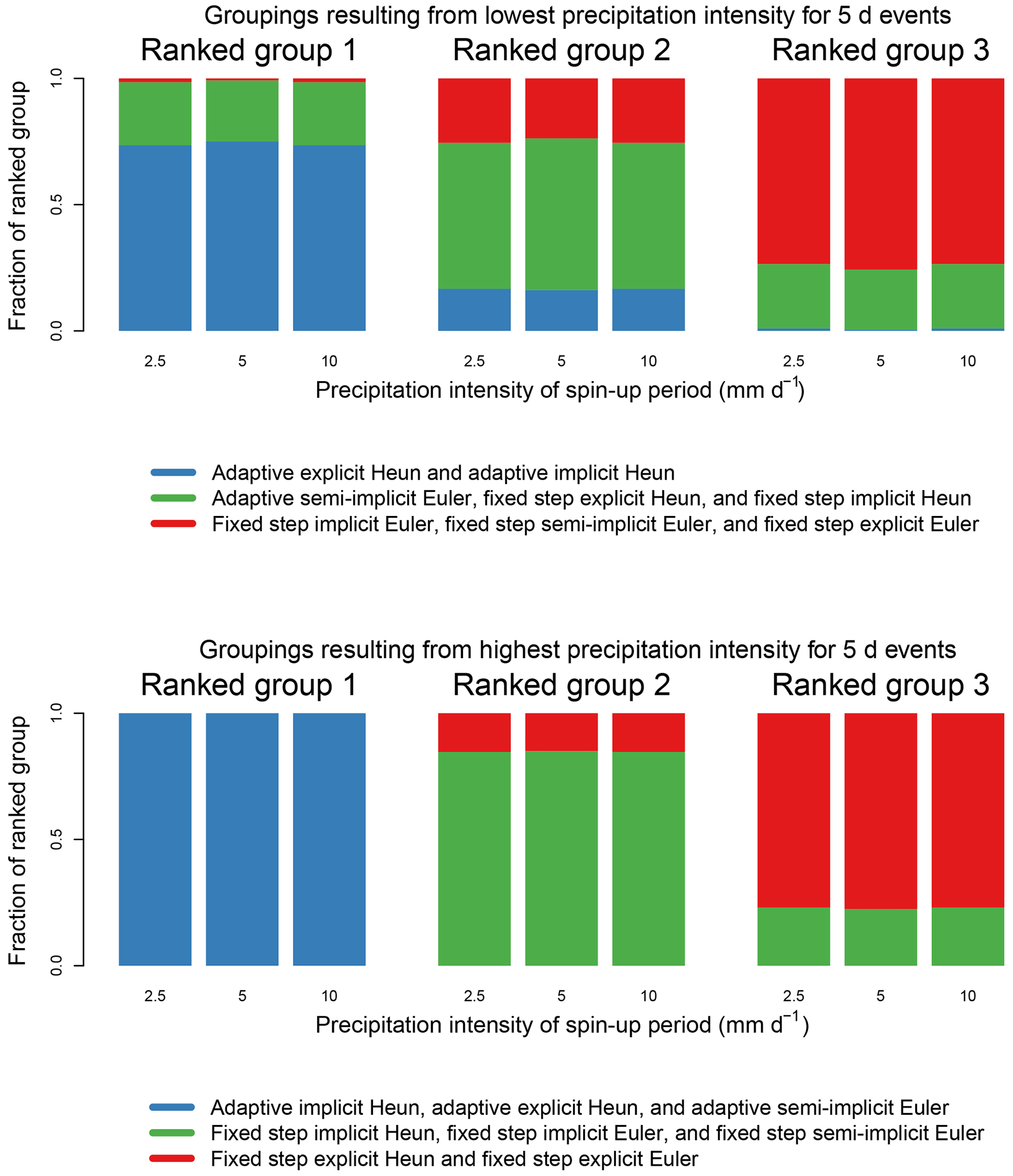
Figure 6The robustness of rankings of numerical techniques in RMSE for high and low precipitation intensity events for three different initial conditions. A ranking is more robust when a selection of numerical methods is prevalent in a given ranked group, indicated by the predominance of a single color in a ranked group. All adaptive methods here use FUSE default error tolerances. These results incorporate hydrographs generated across five model structures and 20 parameter sets. Different rankings are observed for high and low precipitation intensities.
As a concrete example, consider the ranking wherein adaptive second-order methods generally outperform other methods for the least intense 5 d precipitation events. This is reliant upon the adaptive Heun methods occurring often in the ranked group with the lowest error (ranked group 1), given the least intense 5 d precipitation data. To determine how often this is the case, each numerical method in each set of eight runs was given a ranking based on RMSE, where 1 is low error and 8 is high error, and rankings with ties were discarded. Whenever the second-order adaptive methods had either rank 1 or 2 in an individual set of eight runs, they were placed into ranked group 1. As can be seen in Fig. 6, on average, adaptive explicit Heun and adaptive implicit Heun occur in ranked group 1 at a frequency of 74 % across the tested dimensional space for the lowest precipitation intensity for 5 d events, meaning it is usually the case that these two methods as a group have the lowest error for the lowest precipitation intensity for 5 d events. This indicates that the claim “adaptive second-order methods outperform other methods for the least intense 5 d precipitation events” is valid over the majority of the dimensional space tested in Fig. 6 (i.e., it is valid over a variety of choices in model structure, parameter set choice, and initial conditions). Note that there are different rankings for the lowest and highest precipitation intensities, as some numerical methods react very differently to increasing precipitation intensity (described in the previous subsection).
Because the frequency with which methods occurred in their desired groups is generally high, we can be confident that the trends in relative method performance in the previous subsection are usually true over the tested model structures, parameter sets, and initial conditions. The fraction of each ranked group composed of its dominant methods always changed by less than 2 % as a result of changing the initial conditions (see Fig. 6). We can conclude that the rankings are relatively insensitive to initial condition. We determined that the ranking is robust over different model structures as well; the desired ranking was usually observed a high percentage of the time when individual model structures were assessed. However, we found that the model structures containing interflow process representations – namely, FUSE 536, FUSE 550, and FUSE 330 – were less likely than structures without interflow to produce the dominant ranking of Fig. 6 for both the lowest and highest precipitation intensity for 5 d events. The most common deviations from the most common ranking for the lowest precipitation intensity occur due to fixed step implicit Heun outperforming adaptive explicit Heun or adaptive semi-implicit Euler performing approximately as well as the first-order fixed step methods. In order to determine if the rankings were sensitive to the number of parameter sets used, hydrographs were further generated over 80 parameter sets, where the spin-up precipitation intensity was set to 2.5 mm d−1, with no change in the other dimensions. Then, the rankings were compared between the two cases where 80 or 20 parameter sets were used and the spin-up precipitation intensity was 2.5 mm d−1. Because the frequency with which the required ranking is observed changed very little between the two cases – with a largest change for any grouping of 4.9 % – it is evident that the ranking is fairly insensitive to the number of parameter sets used. This indicates that enough parameter sets were used to establish generality over the parameter space. The hydrographs generated over 80 parameter sets were not used beyond investigating ranking robustness.
The same procedure was used to evaluate rankings in computational expense, using number of system flux evaluations rather than RMSE, because further analysis involving computational expense should also be robust over the tested model dimensional space. A total of five distinct ranked groups were discovered. From lowest to highest expense, these groups include the following:
-
fixed step explicit Euler;
-
fixed step explicit Heun;
-
adaptive explicit Heun and fixed step semi-implicit Euler;
-
fixed step implicit Euler, fixed step implicit Heun, and adaptive semi-implicit Euler;
-
adaptive implicit Heun.
This ranking appeared to be common for both low and high precipitation intensity cases. In the style of Fig. 6, and over the same model dimensions, the dominant selection of method(s) never occurred in any ranked group less than 73 % of the time. This indicates that these rankings are robust over a variety of choices in initial condition, parameters, and model structure. Changing either number of parameter sets or initial conditions also always yielded a change in frequency of less than 12 %, demonstrating the insensitivity of computational expense ranking to initial conditions or number of parameter sets used. Based on the results of this subsection, we conclude that the impact of model structure, different parameter sets, and initial conditions on the ranking of numerical methods based on numerical error or computational expense is limited.
4.3 Impact of event duration on error
It was found that longer-duration events have lower associated RMSE, where the median RMSE across all methods decreases with increasing duration. This was analyzed across 20 parameter sets, all five model structures, and for all three spin-up precipitation intensities. The average reduction in median RMSE across all methods between 5 and 20 d events was 74 % for the least intense scaling factor (1 % of interpolated world record average intensity) and 54 % for the most intense scaling factor (120 % of interpolated world record average intensity), where the median RMSE of all individual methods decreased monotonically with increasing precipitation duration. This is, to some extent, a mathematical artifact; because the rainfall signal is flat, a larger portion of a longer time series is closer to an equilibrium discharge. This reduces the average error for the hydrograph. In order to test the extent to which RMSE depends on the geometry of the rainfall signal, the experiment was repeated with new forcing data based on CAMELS precipitation data observed during Hurricane Katrina (Newman et al., 2015). Original forcing data were scaled such that the total precipitation per event is consistent with the rest of the experiment, but relative daily precipitation intensities reflect real data. Under these conditions, the same dominant compositions of ranked groups are observed (and in fact become slightly more robust), and the trend of increasing median RMSE with increasing precipitation intensity is still clear. The decrease in error with increasing duration is still present, though less pronounced, with variable rainfall signals. In this case, the average reduction in median RMSE across all methods between 5 and 20 d events was 69 % for the least intense scaling factor (1 % of interpolated world record total precipitation) and 35 % for the most intense scaling factor (120 % of interpolated world record total precipitation). In either the case of the flat or variable rainfall signal, increasing the duration along an IDF curve necessarily means reducing the daily intensity of the event. Therefore, the reduction in numerical error due to increasing duration might simply be due to the lower daily intensity per event of longer events. Nonetheless, longer-duration events along an IDF curve do represent more total rainfall per event, and it appears as if models yield less error for longer-duration events along an IDF curve (not shown).
4.4 Impact of rainfall signal geometry on error
Here, we present the errors which arise when the experiment is repeated with a variable rainfall signal based on Hurricane Katrina (Newman et al., 2015 and see the previous subsection). Magnitudes of median errors are generally larger with the variable intensity precipitation data but tend to be on the same order of magnitude as in the cases with no variance; because a larger variance in the rainfall signal can increase numerical errors, we can expect that numerical errors in practice might be somewhat larger than reported in the previous subsection. Numerical errors resulting from the 5 d forcing data based on Hurricane Katrina can be found in Fig. 7.
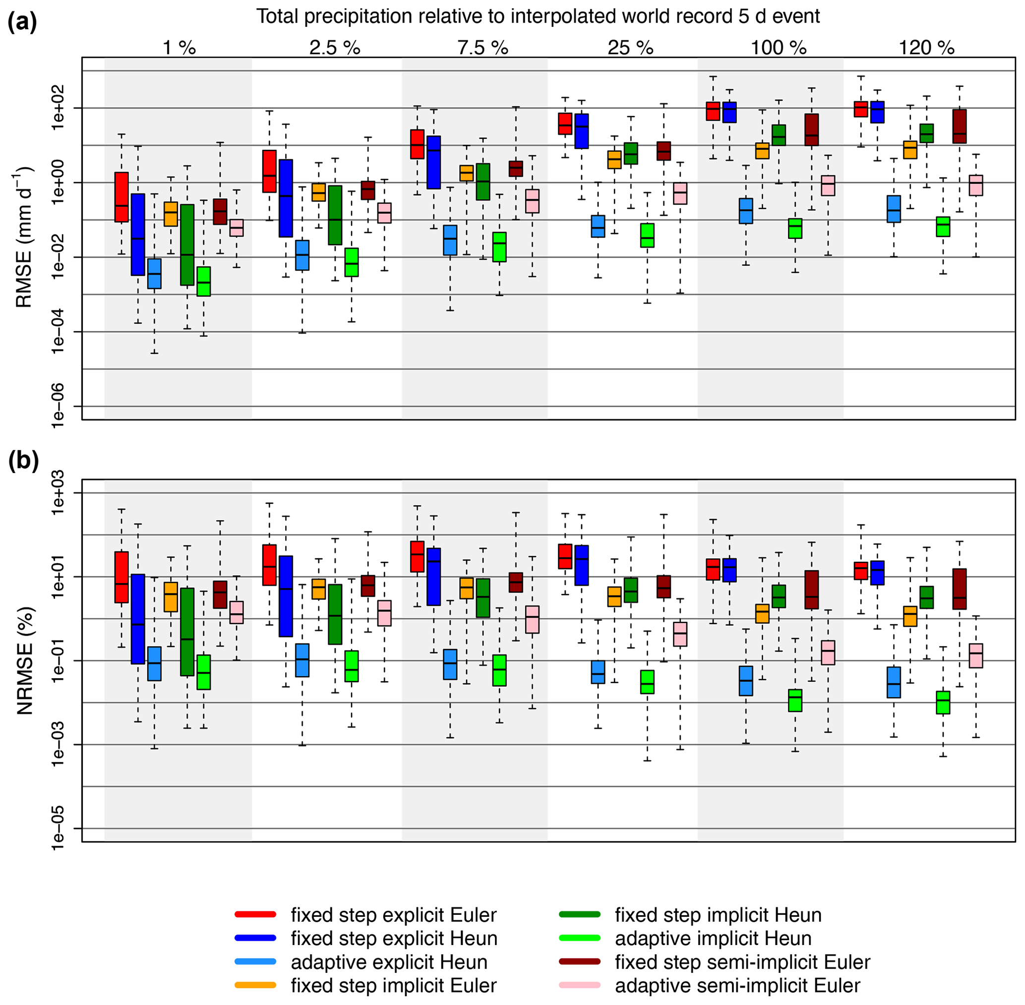
Figure 7Box plots showing the errors (RMSE shown in a and NRMSE shown in b) associated with each numerical technique for 5 d precipitation events of variable intensity with increasing total precipitation, where the total precipitation is represented as a percentage of the interpolated world record 5 d event total precipitation. The solid black line in each box is the median error, the boxes extend to the 25 % and 75 % quantiles, and the whiskers extend to extreme values. All adaptive methods use the FUSE default error tolerances. The model runs represented in this figure are generated across 20 parameter sets, five model structures, and three spin-up conditions. Note that errors are generally larger than in the case where the precipitation signals have no variance per event.
It is also interesting to note that precipitation intensities greater than the 1 d world record event were contained within the variable intensity 5 d forcing data. Because these data generally yield larger errors than with the flat rainfall signals, we can conclude that shorter-duration events incorporating larger intensities can produce larger numerical errors. This further establishes the relationship between numerical error and precipitation intensity and especially underscores the importance of numerical technique choice for intense, short-duration events.
4.5 Computational efficiency
So far, this study makes assessments of numerical errors associated with various numerical techniques. As a result, and with default error tolerances, it seems as if adaptive second-order methods tend to yield the lowest numerical error. Low error is desirable, but computational expense can also be a decisive factor when selecting a numerical method. Figure 8 shows the computational efficiency of the tested numerical techniques. More efficient methods will produce a relatively low median numerical error and will take a relatively small median number of flux evaluations in order to achieve this, i.e., they will occur closer to the leftmost gray line. Mathematically, we can also consider high efficiency to be achieved when the product of number of function calls and numerical error is minimized. We explore multiple error tolerances for the adaptive semi-implicit Euler method. These are examined in order to determine how efficient the adaptive semi-implicit method is when it yields approximately as much error as the adaptive Heun methods with default error tolerances.
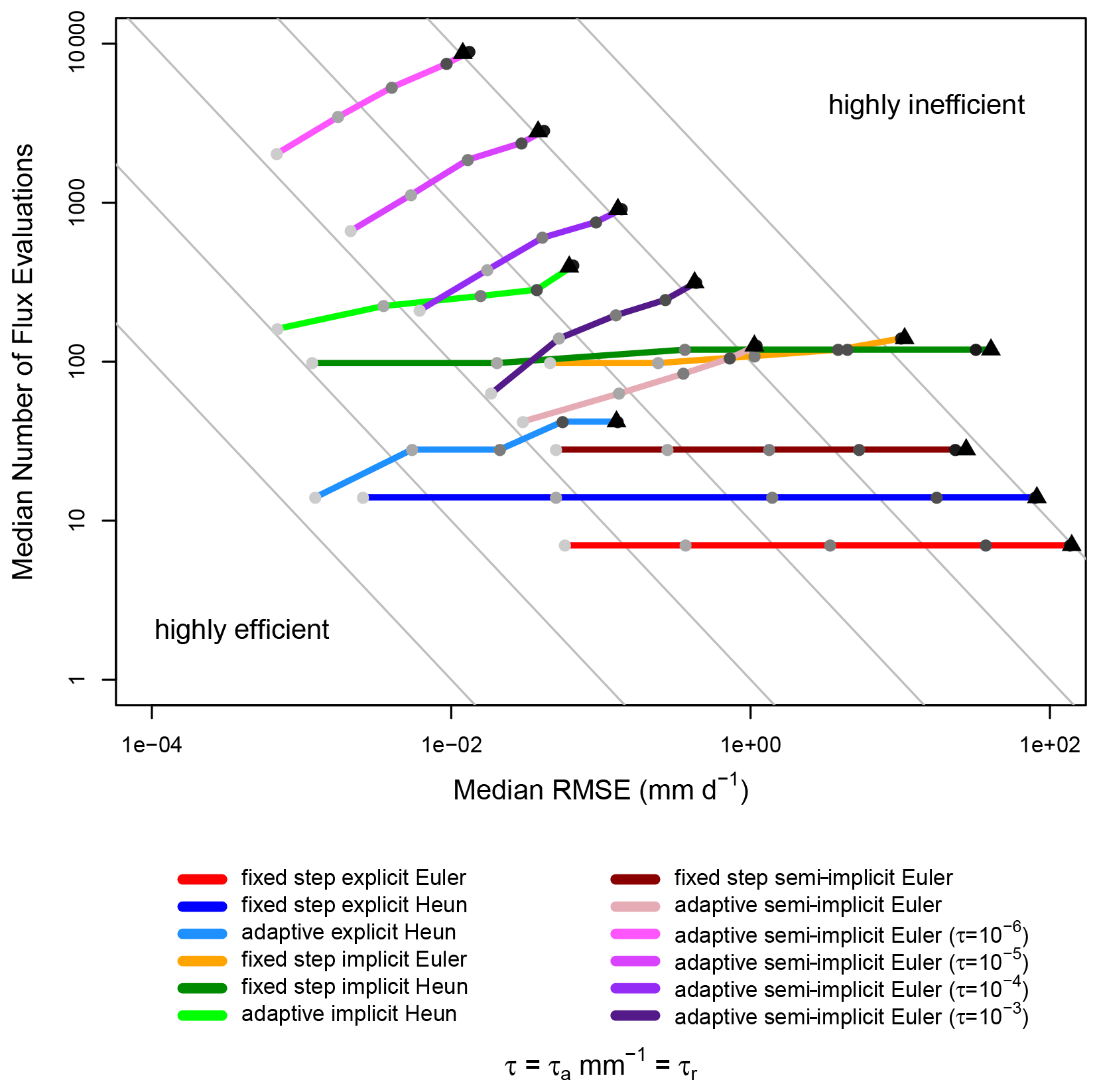
Figure 8Relationship between computational efficiency and the numerical error, where methods are more efficient if they have a low RMSE and a low number of flux evaluations. All medians are calculated across all five model structures, 20 parameter sets, and three spin-up precipitation intensities. All six precipitation intensities for 5 d events are shown, where the light gray dot represents the lowest intensity event, darker gray dots represent increasingly intense precipitation events, and the black triangle represents the highest intensity event. Unless otherwise stated, adaptive methods use the FUSE default tolerances. Purple lines depict adaptive semi-implicit Euler methods with error tolerances below the FUSE default, where the brightest purple method has the smallest error tolerance. Gray lines are visual aids of the form y=, where n is an integer, and x and y, respectively, represent RMSE and number of flux evaluations (gray lines do not represent real data and are used only for visualization purposes). Moving between adjacent gray lines represents an order of magnitude change in efficiency.
Because each precipitation intensity is shown for 5 d events, it is clear that the efficiency of each method tends to decrease with increasing precipitation intensity. Arbitrarily small errors can be achieved with adaptive methods by selecting smaller error tolerances. The semi-implicit method with the smallest error tolerance has the lowest error of any tested numerical method, though this comes at a large computational cost. Adjusting the error tolerances of the adaptive semi-implicit method does not seem to change its efficiency. The central feature of Fig. 8 is that the adaptive explicit Heun method emerges as a clear leader in terms of efficiency, significantly outperforming all other methods for any precipitation intensity. This was also established for the longer-duration events (not shown).
It is possible to examine individual sets of eight runs, rather than median errors and expenses, to determine how often the adaptive explicit Heun method has the highest efficiency. We find that the adaptive explicit Heun method is the most efficient method among those tested 85 % of the time, on average over all 18 forcing data sets, three initial condition levels, 20 parameter sets, and five model structures. When model runs were grouped based on the percentage of world record precipitation intensity, it was found that the percentage of the model runs for which the adaptive explicit Heun method was most efficient ranged between 80.3 % (when precipitation intensities were at 1 % of historical maxima) and 90.1 % (when precipitation intensities were at 25 % of historical maxima).
4.6 Numerical choices control numerical error more than structural choices
Earlier, numerical error was defined as the difference between the exact and the approximate solution to the set of equations composing the model. While numerical error ultimately comes from numerical method choice, the same method in a different model structural context might produce different error magnitudes, so model structure might be able to contribute to numerical error.
A basic analysis of variance (ANOVA) was conducted on NRMSE for all model runs using 20 parameter sets, all three spin-up precipitation intensities, and with all 18 forcing data sets. The p values for groupings based on numerical method choice and structural choice were calculated. The p values for groupings based on the numerical method were always less than , demonstrating that numerical method choice strongly controls NRMSE. The p values for groupings based on structure were below 0.05 for zero of the six 5 d forcing data sets, two of the six 10 d forcing data sets, and three of the six 20 d forcing data sets. The p values for numerical groupings were always lower than the p values for structural groupings. This demonstrates that numerical choices control numerical error more strongly than model structural choices, and structural choices seem to become more important in controlling numerical error for longer duration events.
4.7 Literature review results
Finally, a short literature review was conducted to place the results of this study in context. The surveyed hydrological modeling codes were lumped into three categories (shown in Fig. 9). Presently, we discuss numerical errors that might result from each category.

Figure 9Grouping the reviewed modeling codes (12 in total) into three categories, based on available numerical techniques. Category C codes are the most common.
Of the 12 reviewed codes, one belongs to category A, three belong to category B, and eight belong to category C; the highest order numerical method found in any code was second order. The codes of categories A and B, both having the option of adaptive substepping, can guarantee any level of numerical accuracy with sufficiently small error tolerances. The difference is that the numerical techniques of category B did not include higher-order (second order or higher) adaptive explicit methods and so are not identified as being optimally efficient, according to Fig. 8.
The codes of category C have fixed step solvers. These codes can be further subdivided into more categories, based on the ability or inability to specify a fixed time step, sequential or simultaneous solving, order of numerical method, or implicit or explicit (or other) nature of the numerical methods available. However, the fixed time step either causes an extremely large computational expense when the fixed time step can be arbitrarily set by the user to constrain error (Clark and Kavetski, 2010; Press and Teukolsky, 1992) or relatively large numerical inaccuracies when the time step cannot be adjusted by the user (as shown by this experiment, at least for the daily time step).
The most common method of category C is closely analogous to the fixed step explicit Euler method, albeit in sequential rather than simultaneous form. If willing to accept the flat rainfall signal and chosen dimensional space of Fig. 5 as physically possible, and if willing to accept that FUSE can at least approximately mimic other codes, one could tentatively estimate that category C codes could often yield large median numerical errors from the perspective of RMSE or NRMSE. Specifically, the fixed step explicit Euler method yields a median NRMSE of more than 4 % for 5 d events where the precipitation intensity is 2.5 % of the average intensity for the 5 d historical maximum. This is already fairly large, but median NRMSE for this method can become much larger; by the time precipitation is at 25 % of the world record, numerical NRMSE is over 30 %. Similar trends can be found for longer-duration events, where median errors in RMSE and NRMSE for this method increase with increasing intensity. For 10 and 20 d events, the median NRMSE resulting from the explicit Euler method is maximized at 29 % and 23 %, respectively. When judging a numerical technique by its extremes in error rather than its average, the fixed step explicit Euler method performs poorly; in this experiment, extremes in NRMSE when using this numerical technique easily exceed 100 % for any forcing data set. These results seem to indicate that the most frequently used numerical technique that we encountered in our short survey performs relatively poorly for any precipitation event, where its performance is especially poor for (increasingly common) extreme precipitation events.
5.1 Implications of the study design and further opportunities
5.1.1 Model dimensional space covered
Though the dimensional space tested in this experiment is reasonably large (incorporating various model structures, parameter sets, initial conditions, forcing data, and numerical techniques), it does not cover all possible behaviors of its dimensions. There are model structures in common use outside of the five tested, especially considering that we do not incorporate processes related to freezing or snow. Additionally, we do not use an energy balance; instead, FUSE generates bucket-style hydrological models that only solve a mass balance. Because land surface models incorporate processes involving energy, these might have a different (perhaps more complicated) relationship between numerical error and precipitation extremeness. Furthermore, this experiment incorporates multiple FUSE members (model structures) for generality of results regarding numerical error over multiple structural choices. Our analysis does not extend to determining the extent to which individual physical processes are responsible for numerical error; this presents a clear opportunity for substantial future work. It is important to note that all models generated by FUSE are composed of systems of nonlinear first-order ordinary differential equations; these could have different error characteristics than partial differential equations (such as the Richards equation or shallow wave equations) or higher-order differential equations. Next, even higher-order or differently implemented low-order numerical methods, more initial conditions, less intense precipitations, or longer or shorter precipitation durations remain untested. Still, the results were shown to be rather robust across the fairly broad tested dimensional space, which indicates that extrapolation of the results to other precipitation durations and intensities might be justified.
All rainfall signals in this experiment are either constant with respect to time or are based on a single real event with variance. As such, we do not account for a broad variety of precipitation regimes in terms of variable intensity, which might introduce complexity that is not accounted for in this experiment (Müller-Thomy and Sikorska-Senoner, 2019). However, similar results were obtained with different rainfall signal geometries, indicating that the results might be robust across rainfall geometries. Furthermore, the trends relating numerical error resulting from a numerical method and precipitation extremeness appeared to be rather insensitive to the other tested dimensions, providing robustness to the conclusions.
Because we used a Latin hypercube approach in generating parameter sets and demonstrated that using a larger number of parameter sets did not significantly change the results, we can conclude that we have sufficiently sampled the parameter space. However, in practice, it is likely that most parameters obey a given distribution, which would limit the parameter space which represents physically likely catchments. By sampling broadly rather than using calibrated parameter sets, we do not necessarily represent catchments that are commonly observed. Both approaches have merit; using only calibrated parameter sets might provide a greater assurance that results arise from only physically likely catchments but could bias the results via parameter restriction, while using a broad sampling of the parameter space gives more weight to catchments that might be underrepresented but might not proportionately represent average or common physical settings. Nonetheless, a large variety of parameter combinations is used in Monte Carlo optimization methods regardless of physical realism, which further makes the investigation of numerical error resulting from a broad sampling of parameters worthwhile. While this experiment uses a broad sampling of the parameter space, using only calibrated parameter sets is also a defensible choice – although there is a risk of interaction between numerical error and calibration optimization.
5.1.2 Choices in temporal and spatial discretization
In this experiment, we examine the daily time step because it is commonly used with hydrologic models. However, hydrologic (especially flood) modeling is often carried out at a finer temporal resolution, e.g., hourly (Boithias et al., 2017; Ficchì et al., 2016). If this experiment was repeated with an hourly time step instead of a daily time step, one might expect similar trends in terms of the evolution of numerical error with respect to precipitation intensity and duration, simply with smaller magnitudes of error. This is supported by the theory described in Sect. 2, wherein numerical error is proportional to the time step raised to some integer power. With a smaller time step, one could expect smaller numerical errors, especially for higher-order numerical methods as opposed to lower-order numerical methods (with higher-order numerical methods, numerical error is proportional to the time step raised to a larger integer). Note that this speculative extension of results for a smaller time step also assumes a uniform precipitation intensity. It is possible that, when using real forcing data, rainfall that is locally intense with an hourly temporal resolution could be smoothed out if resampled to the daily temporal resolution. This implies that, with real hourly forcing data, it is possible that a large precipitation intensity which lasts for a short time can produce significant numerical error for a fraction of 1 d; this numerical error might be lessened if the forcing data were aggregated to the daily resolution. Still, the theory presented in Sect. 2 implies that, from a mathematical perspective, one would expect smaller numerical errors when using a smaller time step.
All models in this experiment are lumped rather than distributed and, therefore, do not contain numerical error related to choices in spatial discretization. In a distributed model, numerical error is proportional to the chosen spatial resolution raised to some power and to the time step raised to some power. This theoretically implies that numerical error could potentially increase in terms of maximum value in the context of distributed models under spatially and temporally uniform precipitation. However, a fully distributed model (with real, distributed forcing data) could have its local extremes in space smoothed out given the choice of spatial discretization, while this option is not available for lumped conceptual models. More generally, it is possible for numerical errors due to spatial and temporal discretizations to interact. Therefore, our results are not directly applicable to distributed models. How large the net numerical error is in case of a spatially explicit model, and what controls the magnitude of the errors involved, are interesting subjects for future research. Nonetheless, we tentatively suspect that similar trends might be found in distributed models; namely, that adaptive higher-order methods yield significantly lower numerical error than fixed step lower-order errors do.
5.1.3 Numerical details
Several numerical details remain untested by this experiment. First, FUSE employs embedded error control, which is more efficient than error control requiring extra calculations by about a factor of 2 (Press and Teukolsky, 1992). While we can assume that embedded error control methods are relatively efficient, unembedded methods remain untested, and it is possible that some hydrological models do not use embedded methods. It is possible that this could alter the relative efficiency of various adaptive methods, albeit probably not to a different order of magnitude. Second, all implicit techniques here use a single method to ensure that mass balance errors are sufficiently small; changing the treatment of mass balance errors could lead to somewhat different median computational expenses for implicit methods. However, the median number of flux evaluations per time step under a variety of mass balance error monitoring strategies for fixed step implicit Euler apparently ranges between approximately 8 and 21 (Clark and Kavetski, 2010), where the median number of flux evaluations for fixed step implicit Euler in 5 d events ranges between 14 and 20 (from lowest to highest precipitation intensities) in this experiment. This suggests that the implicit Euler method studied in this paper would probably not achieve a new order of magnitude of efficiency, as shown in Fig. 8, regardless of mass balance error monitoring method. Third, this study does not examine different methods for enforcing solution constraints (e.g., making sure physically impossible storages do not occur as model results). The method for enforcing solution constraints is outlined by Clark and Kavetski (2010), and altering this method could affect numerical error (Shampine et al., 2005). Finally, the adaptive explicit Heun method appears to be the most efficient technique given the limited space of techniques tested; this may no longer be the case when even higher-order adaptive methods are studied. For example, adaptive fourth- or fifth-order Runge–Kutta methods (Schoups et al., 2010) are untested here. A truly optimal solver might be able to dynamically change its order or other options associated with the solver, as in other fields (Karimov et al., 2017; Rackauckas et al., 2020; Lauritzen et al., 2010; Ullrich et al., 2017). Though this point is technically a subset of issues with total dimensional space sampling, testing even higher-order or further modularized numerical techniques would be a straightforward and useful advancement of this work.
5.1.4 Breadth of literature review
The literature review is not an exhaustive survey of all existing modeling codes; instead, it is a smaller investigation of some of the modeling codes that we consider to be widely used. Therefore, it should not be interpreted as a quantitative result of how common numerical errors are but rather a preliminary indication of what might be. Furthermore, note that we only suggest the magnitude and prevalence of errors arising from model runs that are not further scrutinized. Accordingly, our results give an indication of numerical errors arising purely from modeling codes, rather than the occurrence of these errors in published work. For example, it has been demonstrated that fixed step explicit methods are likely to produce large instabilities, but these would probably be identified as such and discarded by the majority of model users.
5.2 Are minimized numerical error and computational expense good metrics with which to choose a numerical method?
At a glance, it might seem as if an inexpensive numerical method with minimized numerical error – the adaptive explicit Heun method – would be an optimal choice for modeling. After all, Clark and Kavetski (2010) do show that numerical error can easily be a large source of error in a model. However, a numerical technique that minimizes numerical error might not always minimize total error in an observational context; in reality, numerical error can cancel out other error sources. This is possible, for example, when a model structure is not sufficiently diffuse, and then a first-order fixed step numerical choice is overly diffuse. The numerical method introduces numerical diffusion (a numerical error), which interacts with the structural error in such a way that the total error is reduced when evaluated on discharge observations, even when compared to a near-exact solution (Clark and Kavetski, 2010). Numerical diffusion has even been intentionally used to represent physical diffusion for increased accuracy (Thober et al., 2019). Furthermore, during calibration, error due to parameter choice can cancel out numerical error, in the same way model structural error can.
Whether or not these are desirable qualities of a numerical method (i.e., whether hydrological models should simply provide accurate predictions of observable data or accurately represent their intended structure regardless of physical realism) is an open question, where the answer is context dependent. On one hand, a more accurate, real-world prediction is ultimately more useful for anyone whose livelihood depends on model results, e.g., a municipality that has to decide whether or not to issue evacuation advisories due to flooding risk. On the other hand, having somewhat unknown errors cancel each other out is a classic instance of finding the right answer for the wrong reasons (Kirchner, 2006), which could pose a problem when the aim of a modeling effort is to gain understanding of hydrological processes. Especially because this experiment shows that model structure can impact numerical error, it is possible that a structural development in a model yielding reduced error is interpreted as an improved representation of nature, where, in reality, the structural development changed the numerical error such that the total error is reduced. When we want to test multiple process-based hypotheses, it would be ideal if we could be more assured that our results are due to the structural changes we make rather than being conflated with numerical error. With this study, we do not claim to have identified optimal methods in an observational context. We do submit, however, that we have identified a few numerical techniques that are desirable (or undesirable) for future process-based hypothesis testing.
5.3 Recommendation for numerical technique
Of the studied methods, this experiment finds that the adaptive explicit Heun method provides the best economy of low error and computational expense on average and, accordingly, is a practical choice for the numerical method. This is consistent with Clark and Kavetski (2010); Kavetski and Clark (2010). However, this study differs in that it does not recommend the fixed step implicit Euler method as an optimal solution, due to the fact that this method, on average, has relatively large numerical error and computational expenses here. The difference in recommendation between the present study and Clark and Kavetski (2010) or Kavetski and Clark (2010) is likely due to two methodological differences. First, Clark and Kavetski (2010); Kavetski and Clark (2010) use the concept of fidelity to determine how closely a numerical technique approximates an exact solution which incorporates real discharge observations. The present study uses purely numerical definitions of error, which are simply different methods. Second, the time periods on which errors were evaluated were different, where the present study evaluates error on the timescale of days, and Clark and Kavetski (2010); Kavetski and Clark (2010) evaluate error on the timescale of years. As this study shows, the RMSE depends on precipitation intensity and duration. It could be the case that the fixed step implicit Euler method produces small numerical errors for a majority of a long time series when precipitation is mild or absent, which would keep the numerical error small on average. In contrast, a shorter but more intense precipitation time series yields larger average numerical errors. On balance, it is encouraging that the present study and the 2010 numerical daemon papers authored by Clark and Kavetski (2010) agree that the fixed step explicit Euler method produces a large amount of error and that the adaptive explicit Heun method is a good choice.
It is further encouraging to see a high degree of similarity between the numerical method recommended by the presented experiment and the recommendation in Schoups et al. (2010). Both works indicate that a second-order explicit adaptive method offers the best intersection of low error and low computational expense. In the case of Schoups et al. (2010), it is further found that the second-order explicit adaptive method is superior to a variety of other methods when calibrating a hydrologic model with Markov chain Monte Carlo methods. This offers additional evidence that second-order explicit adaptive methods are preferred in the simulation of real (rather than just synthetic) streamflow. Furthermore, tasks such as parameter estimation (via calibration) and the simulation of state variables aside from streamflow can be compromised by using the fixed step explicit Euler method (Schoups et al., 2010; Kavetski and Clark, 2010).
5.4 Why are sophisticated numerical methods uncommon in conceptual hydrologic models?
The original numerical daemons papers and other notable work on numerics in hydrologic models (Clark and Kavetski, 2010; Kavetski and Clark, 2010; Schoups et al., 2010) were published over a decade ago; these papers and the present study recommend similar numerical techniques. While some new models use sufficiently advanced numerical methods (Buitink et al., 2020; David et al., 2019; Pilz et al., 2020), it appears as if many current hydrologic models continue to use relatively unsophisticated numerical methods (see Sect. 4.7), where the fixed step explicit Euler method is rather common. Here, we offer some speculative reasoning as to why this might be and indicate an opportunity in hydrologic education with respect to numerical techniques.
Numerical techniques receive substantially more attention in several other environmental sciences disciplines. This is related to the nature of the processes in these disciplines – they may be subject to chaos. That is, small changes in initial conditions or small perturbations will eventually yield wildly different model results. Examples include predator–prey systems (Vano et al., 2006; Inoue and Kamifukumoto, 1984) and meteorological systems, such as the famous Lorenz butterfly (Lorenz, 1963). Attention to numerical schemes is much needed, since the positive feedback loops inherently present in these fields are very sensitive to numerical error. Hydrologic systems of equations, in contrast, tend to contain negative feedback loops. Therefore, numerical errors do not explode – albeit that they are still present, as shown in this study. This stability compared to other fields might offer an explanation for why numerics in hydrology have received relatively little attention. There is clearly a role for hydrology education here, where more attention to numerical techniques can make the next generation of hydrological modelers more aware.
Besides the stability of the hydrological system, another explanation for the limited attention to numerics in hydrology is that numerical error can interact with other sources of error. Multiple sources of error can cancel each other out, such that hydrologic models produce accurate results, despite having significant numerical error. When hydrologic models are working, although not necessarily for the right reasons, there is likely to be less incentive to investigate numerical errors.
In this study, the effects of changing precipitation intensity and duration on the numerical errors and computational expenses resulting from various numerical techniques in the context of lumped hydrological models were examined. Precipitation events varying between 1 % and 120 % of interpolated historical precipitation intensity maxima for various durations were used as forcing data. Model results were generated over a variety of choices in parameters, initial conditions, and model structures for generality. It was found that median root mean square error (RMSE) usually increased with increasing precipitation intensity and decreased with increasing precipitation event duration. Rankings of numerical techniques in terms of RMSE and the number of flux evaluations were established for varying precipitation intensities. These were shown to be robust over the majority of choices in parameters, model structures, and initial conditions. Then, the efficiency of each technique was examined by comparing computational expense and numerical error. Of the tested methods, a clear leader in efficiency emerged for all precipitation intensities, namely the adaptive explicit Heun method. A small literature review was conducted on various hydrological modeling codes, demonstrating that this method, and even adaptive methods in general, might be uncommon in practice, and that a much more numerically erroneous method might be common. Because process-based hydrological knowledge is enhanced by reductions in numerical error and computational expense, and because numerical errors are in many areas likely to increase with the changing climate (via more extreme precipitation), we advocate a more widespread use of highly efficient numerical methods.
The MMFs reviewed for this study were the Modular Assessment of Rainfall–Runoff Models Toolbox (MARRMoT; Knoben, 2018; Knoben et al., 2019), the Structure for Unifying Multiple Modeling Alternatives (SUMMA; NCAR, 2017; Clark et al., 2015), Raven (Snowdon, 2010; Craig et al., 2020), the Framework for Understanding Structural Errors (FUSE; Clark et al., 2008; Clark and Kavetski, 2010), and SUPERFLEX (Fenicia et al., 2011). The models reviewed for this study included the Variable Infiltration Capacity model (VIC; University of Washington, 2016; Hamman et al., 2018), the mesoscale Hydrological model (mHM; Zink and Cuntz, 2013; Samaniego et al., 2010), dynamic TOPMODEL (Buytaert, 2018; Metcalfe et al., 2015; Kavetski et al., 2003), the Precipitation Runoff Modelling System (PRMS; Markstrom et al., 2015), the Génie Rural model à 4 paramètres Journaliers (GR4J; Perrin et al., 2003; Santos et al., 2018), the Sacramento soil moisture accounting model (Finnerty et al., 1997; Burnash et al., 1973; Koren et al., 2014), and Hydrologiska Byråns Vattenbalansavdelning (HBV) light (Reynolds et al., 2017). More information about the numerical methods used by each code can be found in the Supplement. Note that this literature review was performed in the first half of 2020; it is possible that modeling codes have received updates to their numerical methods since then.
The data used in producing this paper are available at https://doi.org/10.4211/hs.acf9a56e93bc4863b972e1e8af36dc0c (La Follette, 2021).
The supplement related to this article is available online at: https://doi.org/10.5194/hess-25-5425-2021-supplement.
PTL wrote the paper, ran FUSE, and developed many of the types of analysis present. LAM and AJT supervised the project; this project began as PTL's thesis towards a Masters in Science. LAM acted as primary supervisor and AJT secondary. Both LAM and AJT developed the original concept of investigating how numerical error in hydrological models changed with respect to precipitation extremeness and provided extensive feedback as the paper was written. LAM also wrote several paragraphs in the paper during revision. NA provided extensive technical support for setting up FUSE, and a number of insightful comments about halfway through the writing process, which led to new analyses. MC provided critical support regarding conceptual understanding of first-order adaptive techniques, together with comments and suggestions which improved the way in which initial conditions were set. KJ provided necessary information for the literature review (along with PL), together with reviews throughout the writing process.
The authors declare that they have no conflict of interest.
Publisher's note: Copernicus Publications remains neutral with regard to jurisdictional claims in published maps and institutional affiliations.
The authors would like to acknowledge Stephan Thober, for vital information about the numerical techniques of various reviewed codes, Chiel van Heerwaarden, for information on numerical practices outside of hydrology, Karin van der Wiel, for discussions about the nature of extreme rainfall, and Tim van Emmerik, for suggestions about forcing precipitation intensity.
This paper was edited by Nadav Peleg and reviewed by Jasper Vrugt, Martina Kauzlaric, and one anonymous referee.
Addor, N. and Melsen, L.: Legacy, rather than adequacy, drives the selection of hydrological models, Water Resour. Res., 55, 378–390, 2019. a, b, c
Addor, N., Jaun, S., Fundel, F., and Zappa, M.: An operational hydrological ensemble prediction system for the city of Zurich (Switzerland): skill, case studies and scenarios, Hydrol. Earth Syst. Sci., 15, 2327–2347, https://doi.org/10.5194/hess-15-2327-2011, 2011. a
Blake, E. S. and Zelinsky, D. A.: National Hurricane Center tropical cyclone report hurricane Harvey, available at: https://www.nhc.noaa.gov/data/tcr/index.php?season=2017&basin=atl (last access: 1 May 2021), 2018. a
Boithias, L., Sauvage, S., Lenica, A., Roux, H., Abbaspour, K. C., Larnier, K., Dartus, D., and Sánchez-Pérez, J. M.: Simulating flash floods at hourly time-step using the SWAT model, Water, 9, 929, https://doi.org/10.3390/w9120929, 2017. a
Brauer, C. C., Teuling, A. J., Overeem, A., van der Velde, Y., Hazenberg, P., Warmerdam, P. M. M., and Uijlenhoet, R.: Anatomy of extraordinary rainfall and flash flood in a Dutch lowland catchment, Hydrol. Earth Syst. Sci., 15, 1991–2005, https://doi.org/10.5194/hess-15-1991-2011, 2011. a
Buitink, J., Melsen, L. A., Kirchner, J. W., and Teuling, A. J.: A distributed simple dynamical systems approach (dS2 v1.0) for computationally efficient hydrological modelling at high spatio-temporal resolution, Geosci. Model Dev., 13, 6093–6110, https://doi.org/10.5194/gmd-13-6093-2020, 2020. a
Burnash, R., Ferral, R., and McGuire, R.: A generalised streamflow simulation system–conceptual modelling for digital computers, Tech. rep., Joint Federal and State River Forecast Center, Sacramento, 1973. a
Buytaert, W.: Implementation of the Hydrological Model TOPMODEL in R, available at: https://cran.r-project.org/web/packages/topmodel/topmodel.pdf (last access: 1 May 2021), 2018. a
Clark, M. P. and Kavetski, D.: Ancient numerical daemons of conceptual hydrological modeling: 1. Fidelity and efficiency of time stepping schemes, Water Resour. Res., 46, W10510, https://doi.org/10.1029/2009WR008894, 2010. a, b, c, d, e, f, g, h, i, j, k, l, m, n, o, p, q, r, s, t, u, v, w
Clark, M. P., Slater, A. G., Rupp, D. E., Woods, R. A., Vrugt, J. A., Gupta, H. V., Wagener, T., and Hay, L. E.: Framework for Understanding Structural Errors (FUSE): A modular framework to diagnose differences between hydrological models, Water Resour. Res., 44, W00B02, https://doi.org/10.1029/2007WR006735, 2008. a, b
Clark, M. P., Nijssen, B., Lundquist, J. D., Kavetski, D., Rupp, D. E., Woods, R. A., Freer, J. E., Gutmann, E. D., Wood, A. W., Brekke, L. D., Arnold, J. R., Gochis, D. J., and Rasmussen, R. M.: A unified approach for process-based hydrologic modeling: 1. Modeling concept, Water Resour. Res., 51, 2498–2514, 2015. a
Coxon, G., Freer, J., Wagener, T., Odoni, N., and Clark, M.: Diagnostic evaluation of multiple hypotheses of hydrological behaviour in a limits-of-acceptability framework for 24 UK catchments, Hydrol. Process., 28, 6135–6150, 2014. a
Coxon, G., Freer, J., Lane, R., Dunne, T., Knoben, W. J. M., Howden, N. J. K., Quinn, N., Wagener, T., and Woods, R.: DECIPHeR v1: Dynamic fluxEs and ConnectIvity for Predictions of HydRology, Geosci. Model Dev., 12, 2285–2306, https://doi.org/10.5194/gmd-12-2285-2019, 2019. a
Craig, J. R., Brown, G., Chlumsky, R., Jenkinson, W., Jost, G., Lee, K., Mai, J., Serrer, M., Snowdon, A. P., Sgro, N., Shafii, M., Snowdon, A. P., and Tolson, B. A.: Flexible watershed simulation with the Raven hydrological modelling framework, Environ. Modelling Softw., 129, 104728, https://doi.org/10.1016/j.envsoft.2020.104728, 2020. a
David, P. C., Oliveira, D. Y., Grison, F., Kobiyama, M., and Chaffe, P. L.: Systematic increase in model complexity helps to identify dominant streamflow mechanisms in two small forested basins, Hydrolog. Sci. J., 64, 455–472, 2019. a
Dralle, D. N., Hahm, W. J., Rempe, D. M., Karst, N. J., Thompson, S. E., and Dietrich, W. E.: Quantification of the seasonal hillslope water storage that does not drive streamflow, Hydrol. Process., 32, 1978–1992, 2018. a
Fenicia, F., Kavetski, D., and Savenije, H. H.: Elements of a flexible approach for conceptual hydrological modeling: 1. Motivation and theoretical development, Water Resour. Res., 47, W11510, https://doi.org/10.1029/2010WR010174, 2011. a
Ficchì, A., Perrin, C., and Andréassian, V.: Impact of temporal resolution of inputs on hydrological model performance: An analysis based on 2400 flood events, J. Hydrol., 538, 454–470, 2016. a
Finnerty, B. D., Smith, M. B., Seo, D.-J., Koren, V., and Moglen, G. E.: Space-time scale sensitivity of the Sacramento model to radar-gage precipitation inputs, J. Hydrol., 203, 21–38, 1997. a
Glowinski, R., Osher, S J., and Yin, W.: Splitting methods in communication, imaging, science, and engineering, Springer, Cham, Switzerland, 2017. a, b
Gupta, H. V., Kling, H., Yilmaz, K. K., and Martinez, G. F.: Decomposition of the mean squared error and NSE performance criteria: Implications for improving hydrological modelling, J. Hydrol., 377, 80–91, 2009. a
Hamman, J. J., Nijssen, B., Bohn, T. J., Gergel, D. R., and Mao, Y.: The Variable Infiltration Capacity model version 5 (VIC-5): infrastructure improvements for new applications and reproducibility, Geosci. Model Dev., 11, 3481–3496, https://doi.org/10.5194/gmd-11-3481-2018, 2018. a
Higham, N. J.: Accuracy and stability of numerical algorithms, in: vol. 80, Siam, University Science Center, Philadelphia, PA, 2002. a
Huang, X., Swain, D. L., and Hall, A. D.: Future precipitation increase from very high resolution ensemble downscaling of extreme atmospheric river storms in California, Sci. Adv., 6, eaba1323, https://doi.org/10.1126/sciadv.aba1323, 2020. a
Inoue, M. and Kamifukumoto, H.: Scenarios leading to chaos in a forced Lotka-Volterra model, Prog. Theor. Phys., 71, 930–937, 1984. a
Jameson, A. and Turkel, E.: Implicit schemes and LU Decompositions, Math. Comput., 37, 385–397, 1981. a, b
Jasper, K., Gurtz, J., and Lang, H.: Advanced flood forecasting in Alpine watersheds by coupling meteorological observations and forecasts with a distributed hydrological model, J. Hydrol., 267, 40–52, 2002. a, b, c
Karimov, A. I., Butusov, D. N., and Tutueva, A. V.: Adaptive explicit-implicit switching solver for stiff ODEs, in: 2017 IEEE Conference of Russian Young Researchers in Electrical and Electronic Engineering (EIConRus), February 2017, St. Petersburg, Russia, 440–444, 2017. a
Kavetski, D. and Clark, M. P.: Ancient numerical daemons of conceptual hydrological modeling: 2. Impact of time stepping schemes on model analysis and prediction, Water Resour. Res., 46, W10511, https://doi.org/10.1029/2009WR008896, 2010. a, b, c, d, e, f, g, h, i
Kavetski, D., Binning, P., and Sloan, S. W.: Noniterative time stepping schemes with adaptive truncation error control for the solution of Richards equation, Water Resour. Res., 38, 29-1–29-10, 2002. a, b
Kavetski, D., Kuczera, G., and Franks, S. W.: Semidistributed hydrological modeling: A “saturation path” perspective on TOPMODEL and VIC, Water Resour. Res., 39, 1246, https://doi.org/10.1029/2003WR002122, 2003. a
Kavetski, D., Kuczera, G., and Franks, S. W.: Bayesian analysis of input uncertainty in hydrological modeling: 1. Theory, Water Resour. Res., 42, W03407, https://doi.org/10.1029/2005WR004368, 2006a. a
Kavetski, D., Kuczera, G., and Franks, S. W.: Bayesian analysis of input uncertainty in hydrological modeling: 2. Application, Water Resour. Res., 42, W03408, https://doi.org/10.1029/2005WR004376, 2006b. a
Kirchner, J. W.: Getting the right answers for the right reasons: Linking measurements, analyses, and models to advance the science of hydrology, Water Resour. Res., 42, W03S04, https://doi.org/10.1029/2005WR004362, 2006. a
Kirchner, J. W.: Catchments as simple dynamical systems: Catchment characterization, rainfall-runoff modeling, and doing hydrology backward, Water Resour. Res., 45, W02429, https://doi.org/10.1029/2008WR006912, 2009. a
Kittel, C. M. M., Nielsen, K., Tøttrup, C., and Bauer-Gottwein, P.: Informing a hydrological model of the Ogooué with multi-mission remote sensing data, Hydrol. Earth Syst. Sci., 22, 1453–1472, https://doi.org/10.5194/hess-22-1453-2018, 2018. a
Knoben, W.: wknoben/MARRMoT, GitHub [code], available at: https://github.com/wknoben/MARRMoT/tree/master/MARRMoT/Functions/Time stepping (last access: 6 October 2021), 2018. a
Knoben, W. J. M., Freer, J. E., Fowler, K. J. A., Peel, M. C., and Woods, R. A.: Modular Assessment of Rainfall–Runoff Models Toolbox (MARRMoT) v1.2: an open-source, extendable framework providing implementations of 46 conceptual hydrologic models as continuous state-space formulations, Geosci. Model Dev., 12, 2463–2480, https://doi.org/10.5194/gmd-12-2463-2019, 2019. a
Koren, V., Smith, M., and Cui, Z.: Physically-based modifications to the Sacramento Soil Moisture Accounting model. Part A: Modeling the effects of frozen ground on the runoff generation process, J. Hydrol., 519, 3475–3491, 2014. a
La Follette, P.: Data for La Follette et al (Numerical Daemons and extreme precipitation) [data set], available at: http://www.hydroshare.org/resource/acf9a56e93bc4863b972e1e8af36dc0c, last access: 6 October 2021. a
Lauritzen, P. H., Jablonowski, C., Taylor, M. A., and Nair, R. D.: Rotated versions of the Jablonowski steady-state and baroclinic wave test cases: A dynamical core intercomparison, J. Adv. Model. Earth Syst., 2, 15, https://doi.org/10.3894/JAME S.2010.2.15, 2010. a
Lorenz, E. N.: Deterministic nonperiodic flow, J. Atmos. Sci., 20, 130–141, 1963. a
Madsen, H., Lawrence, D., Lang, M., Martinkova, M., and Kjeldsen, T.: Review of trend analysis and climate change projections of extreme precipitation and floods in Europe, J. Hydrology, 519, 3634–3650, 2014. a
Markstrom, S. L., Regan, R. S., Hay, L. E., Viger, R. J., Webb, R. M., Payn, R. A., and LaFontaine, J. H.: PRMS-IV, the precipitation-runoff modeling system, version 4, US Geological Survey Techniques and Methods, US Geological Survey, Reston, Virginia, 2015. a
McMillan, H., Krueger, T., and Freer, J.: Benchmarking observational uncertainties for hydrology: rainfall, river discharge and water quality, Hydrol. Process., 26, 4078–4111, https://doi.org/10.1002/hyp.9384, 2012. a
McMillan, H., Seibert, J., Petersen-Overleir, A., Lang, M., White, P., Snelder, T., Rutherford, K., Krueger, T., Mason, R., and Kiang, J.: How uncertainty analysis of streamflow data can reduce costs and promote robust decisions in water management applications, Water Resour. Res., 53, 5220–5228, https://doi.org/10.1002/2016WR020328, 2017. a
Meehl, G. A., Arblaster, J. M., and Tebaldi, C.: Understanding future patterns of increased precipitation intensity in climate model simulations, Geophys. Res. Lett., 32, L18719, https://doi.org/10.1029/2005GL023680, 2005. a
Melsen, L. and Guse, B.: Hydrological drought simulations: How climate and model structure control parameter sensitivity, Water Resour. Res., 55, 10527–10547, 2019. a
Melsen, L. A., Addor, N., Mizukami, N., Newman, A. J., Torfs, P. J. J. F., Clark, M. P., Uijlenhoet, R., and Teuling, A. J.: Mapping (dis)agreement in hydrologic projections, Hydrol. Earth Syst. Sci., 22, 1775–1791, https://doi.org/10.5194/hess-22-1775-2018, 2018. a, b
Metcalfe, P., Beven, K., and Freer, J.: Dynamic TOPMODEL: A new implementation in R and its sensitivity to time and space steps, Environ. Model. Softw., 72, 155–172, 2015. a
Müller-Thomy, H. and Sikorska-Senoner, A. E.: Does the complexity in temporal precipitation disaggregation matter for a lumped hydrological model?, Hydrolog. Sci. J., 64, 1453–1471, 2019. a
Nash, J. E. and Sutcliffe, J. V.: River flow forecasting through conceptual models part I – A discussion of principles, J. Hydrol., 10, 282–290, 1970. a
NCAR: NCAR/summa, GitHub [code], available at: https://github.com/CH-Earth/summa/tree/master/docs/input_output (last access: 6 October 2021), 2017. a
Newman, A. J., Clark, M. P., Sampson, K., Wood, A., Hay, L. E., Bock, A., Viger, R. J., Blodgett, D., Brekke, L., Arnold, J. R., Hopson, T., and Duan, Q.: Development of a large-sample watershed-scale hydrometeorological data set for the contiguous USA: data set characteristics and assessment of regional variability in hydrologic model performance, Hydrol. Earth Syst. Sci., 19, 209–223, https://doi.org/10.5194/hess-19-209-2015, 2015. a, b
NOAA: California Nevada River Forecast Center [data set], available at: https://www.cnrfc.noaa.gov/archivePrecipMap.php?area=sf&month=02&day=27&year=19 (last access: 6 October 2021), 2019. a
Noh, S. J., Rakovec, O., Weerts, A. H., and Tachikawa, Y.: On noise specification in data assimilation schemes for improved flood forecasting using distributed hydrological models, J. Hydrol., 519, 2707–2721, 2014. a
Paton, F., Maier, H., and Dandy, G.: Relative magnitudes of sources of uncertainty in assessing climate change impacts on water supply security for the southern Adelaide water supply system, Water Resour. Res., 49, 1643–1667, 2013. a
Perrin, C., Michel, C., and Andréassian, V.: Improvement of a parsimonious model for streamflow simulation, J. Hydrol., 279, 275–289, 2003. a
Pilz, T., Francke, T., Baroni, G., and Bronstert, A.: How to Tailor My Process-Based Hydrological Model? Dynamic Identifiability Analysis of Flexible Model Structures, Water Resourc. Res., 56, e2020WR028042, https://doi.org/10.1029/2020WR028042, 2020. a
Prancevic, J. P. and Kirchner, J. W.: Topographic controls on the extension and retraction of flowing streams, Geophys. Res. Lett., 46, 2084–2092, 2019. a
Prein, A. F., Rasmussen, R. M., Ikeda, K., Liu, C., Clark, M. P., and Holland, G. J.: The future intensification of hourly precipitation extremes, Nat. Clim. Change, 7, 48–52, 2017. a
Press, W. H. and Teukolsky, S. A.: Adaptive Stepsize Runge-Kutta Integration, Comput. Phys., 6, 188–191, 1992. a, b, c, d
Rackauckas, C., Ranocha, H., Thakur, D., et al.: ODE Solvers, GitHub [code], available at: https://github.com/SciML/DiffEqDocs.jl/blob/master/docs/src/solvers/ode_solve.md (last access: 6 October 2021), 2020. a
Ralph, F. M., Cannon, F., Tallapragada, V., Davis, C. A., Doyle, J. D., Pappenberger, F., Subramanian, A., Wilson, A. M., Lavers, D. A., Reynolds, C. A., Haase, J. S., Centurioni, L., Ingleby, B., Rutz, J. J., Cordeira, J. M., Zheng, M., Hecht, C., Kawzenuk, B., and Delle Monache, L.: West Coast forecast challenges and development of atmospheric river reconnaissance, B. Am. Meteorol. Soc., 101, E1357–E1377, 2020. a
Refsgaard, J. C.: Parameterisation, calibration and validation of distributed hydrological models, J. Hydrol., 198, 69–97, 1997. a
Refsgaard, J. C. and Knudsen, J.: Operational validation and intercomparison of different types of hydrological models, Water Resour. Res., 32, 2189–2202, 1996. a
Rempe, D. M. and Dietrich, W. E.: A bottom-up control on fresh-bedrock topography under landscapes, P. Natl. Acad. Sci. USA, 111, 6576–6581, 2014. a
Reynolds, J., Halldin, S., Xu, C.-Y., Seibert, J., and Kauffeldt, A.: Sub-daily runoff predictions using parameters calibrated on the basis of data with a daily temporal resolution, J. Hydrol., 550, 399–411, 2017. a
Samaniego, L., Kumar, R., and Attinger, S.: Multiscale parameter regionalization of a grid-based hydrologic model at the mesoscale, Water Resour. Res., 46, W05523, https://doi.org/10.1029/2008WR007327, 2010. a
Santos, L., Thirel, G., and Perrin, C.: Continuous state-space representation of a bucket-type rainfall-runoff model: a case study with the GR4 model using state-space GR4 (version 1.0), Geosci. Model Dev., 11, 1591–1605, https://doi.org/10.5194/gmd-11-1591-2018, 2018. a
Schoups, G., Vrugt, J., Fenicia, F., and Van de Giesen, N.: Corruption of accuracy and efficiency of Markov chain Monte Carlo simulation by inaccurate numerical implementation of conceptual hydrologic models, Water Resour. Res., 46, W10530, https://doi.org/10.1029/2009WR008648, 2010. a, b, c, d, e, f
Seneviratne, S. I., Nicholls, N., Easterling, D., Goodess, C. M., Kanae, S., Kossin, J., Luo, Y., Marengo, J., McInnes, K., Rahimi, M., Reichstein, M., Sorteberg, A., Vera, C., Zhang, X., Alexander, L. V., Allen, S., Benito, G., Cavazos, T., Clague, J., Conway, D., Della-Marta, P. M., Gerber, M., Gong, S., Goswami, B. N., Hemer, M., Huggel, C., van den Hurk, B., Kharin, V. V., Kitoh, A., Klein Tank, A. M. G., Li, G., Mason, S. J., McGuire, W., van Oldenborgh, G. J., Orlowsky, B., Smith, S., Thiaw, W., Velegrakis, A., Yiou, P., Zhang, T., Zhou, T., and Zwiers, F. W.: Changes in climate extremes and their impacts on the natural physical environment, Cambridge University Press, Cambridge, UK and New York, NY, USA, 2017. a
Shampine, L. F., Thompson, S., Kierzenka, J., and Byrne, G.: Non-negative solutions of ODEs, Appl. Math. Comput., 170, 556–569, 2005. a
Snowdon, A.: Improved numerical methods for distributed hydrological models, MS thesis, University of Waterloo, Waterloo, 2010. a
Süli, E. and Mayers, D. F.: An introduction to numerical analysis, Cambridge University Press, Cambridge, 2003. a, b, c
Thober, S., Cuntz, M., Kelbling, M., Kumar, R., Mai, J., and Samaniego, L.: The multiscale routing model mRM v1.0: simple river routing at resolutions from 1 to 50 km, Geosci. Model Dev., 12, 2501–2521, https://doi.org/10.5194/gmd-12-2501-2019, 2019. a
Trenberth, K. E.: Changes in precipitation with climate change, Clim. Res., 47, 123–138, 2011. a
Ullrich, P. A., Jablonowski, C., Kent, J., Lauritzen, P. H., Nair, R., Reed, K. A., Zarzycki, C. M., Hall, D. M., Dazlich, D., Heikes, R., Konor, C., Randall, D., Dubos, T., Meurdesoif, Y., Chen, X., Harris, L., Kühnlein, C., Lee, V., Qaddouri, A., Girard, C., Giorgetta, M., Reinert, D., Klemp, J., Park, S.-H., Skamarock, W., Miura, H., Ohno, T., Yoshida, R., Walko, R., Reinecke, A., and Viner, K.: DCMIP2016: a review of non-hydrostatic dynamical core design and intercomparison of participating models, Geosci. Model Dev., 10, 4477–4509, https://doi.org/10.5194/gmd-10-4477-2017, 2017. a
University of Washington: Frequently Asked Questions [code], available at: https://vic.readthedocs.io/en/master/FAQ/FAQ/ (last access: 6 October 2021), 2016. a
Vano, J., Wildenberg, J., Anderson, M., Noel, J., and Sprott, J.: Chaos in low-dimensional Lotka–Volterra models of competition, Nonlinearity, 19, 2391, https://doi.org/10.1088/0951-7715/19/10/006, 2006. a
Vrugt, J. A., ter Braak, C. J. F., Clark, M. P., Hyman, J. M., and Robinson, B. A.: Treatment of input uncertainty in hydrologic modeling: Doing hydrology backward with Markov chain Monte Carlo simulation, Water Resour. Res., 44, W00B09, https://doi.org/10.1029/2007WR006720, 2008. a
Weerts, A. H. and El Serafy, G. Y.: Particle filtering and ensemble Kalman filtering for state updating with hydrological conceptual rainfall-runoff models, Water Resour. Res., 42, W09403, https://doi.org/10.1029/2005WR004093, 2006. a, b
Westerberg, I., Guerrero, J., Seibert, J., Beven, K. J., and Halldin, S.: Stage-discharge uncertainty derived with a non-stationary rating curve in the Choluteca River, Honduras, Hydrol. Process., 25, 603–613, https://doi.org/10.1002/hyp.7848, 2011. a
Wood, S. J., Jones, D. A., and Moore, R. J.: Accuracy of rainfall measurement for scales of hydrological interest, Hydrol. Earth Syst. Sci., 4, 531–543, https://doi.org/10.5194/hess-4-531-2000, 2000. a
World Meteorological Organization: Guide to hydrological practices, Secretariat of the World Meteorological Organization [data set], http://www.bom.gov.au/water/designRainfalls/rainfallEvents/worldRecRainfall.shtml (last access: 6 October 2021), 1994. a, b, c
Wrede, S., Fenicia, F., Martínez-Carreras, N., Juilleret, J., Hissler, C., Krein, A., Savenije, H. H., Uhlenbrook, S., Kavetski, D., and Pfister, L.: Towards more systematic perceptual model development: a case study using 3 Luxembourgish catchments, Hydrol. Process., 29, 2731–2750, 2015. a, b, c
Zink, M. and Cuntz, M.: mhm.nml ⋅ develop ⋅ mhm/mhm [code], available at: https://git.ufz.de/mhm/mhm/blob/develop/mhm.nml (last access: 6 October 2021), 2013. a
- Abstract
- Introduction
- Overview of numerical methods used for approximating differential equation solutions in this experiment
- Methods
- Results
- Discussion
- Conclusions
- Appendix A: Reviewed codes
- Data availability
- Author contributions
- Competing interests
- Disclaimer
- Acknowledgements
- Review statement
- References
- Supplement