the Creative Commons Attribution 4.0 License.
the Creative Commons Attribution 4.0 License.
 | 02 Feb 2021
Estimation of hydrological drought recovery based on precipitation and Gravity Recovery and Climate Experiment (GRACE) water storage deficit
John Thomas Reager
Ali Behrangi
Drought is a natural extreme climate phenomenon that presents great challenges in forecasting and monitoring for water management purposes. Previous studies have examined the use of Gravity Recovery and Climate Experiment (GRACE) terrestrial water storage anomalies to measure the amount of water missing from a drought-affected region, and other studies have attempted statistical approaches to drought recovery forecasting based on joint probabilities of precipitation and soil moisture. The goal of this study is to combine GRACE data and historical precipitation observations to quantify the amount of precipitation required to achieve normal storage conditions in order to estimate a likely drought recovery time. First, linear relationships between terrestrial water storage anomaly (TWSA) and cumulative precipitation anomaly are established across a range of conditions. Then, historical precipitation data are statistically modeled to develop simplistic precipitation forecast skill based on climatology and long-term trend. Two additional precipitation scenarios are simulated to predict the recovery period by using a standard deviation in climatology and long-term trend. Precipitation scenarios are convolved with water deficit estimates (from GRACE) to calculate the best estimate of a drought recovery period. The results show that, in the regions of strong seasonal amplitude (like a monsoon belt), drought continues even with above-normal precipitation until its wet season. The historical GRACE-observed drought recovery period is used to validate the approach. Estimated drought for an example month demonstrated an 80 % recovery period, as observed by the GRACE.
- Article
(15868 KB) - Full-text XML
-
Supplement
(2452 KB) - BibTeX
- EndNote


Drought is a widespread recurring natural hazard with several direct and indirect impacts. The shortage of water in an ecosystem not only reduces water availability for human consumption but also causes extensive flora and fauna mortality. Dry land, with little vegetation on the surface, increases soil erosion, reduces water resilience time and enhances the possibility of forest fires, leading to many indirect disasters. Big historical droughts have affected millions of lives and cost billions of dollars in the last half century. For example, the 1988 USA drought is estimated to have cost USD 40 billion, and the 1999 drought in Asia affected 60 million people (Mishra and Singh, 2010). Severe water crises can put society in turmoil and drive large-scale migrations, particularly in the developing parts of the world, e.g., the 2011 East African drought (Lyon and DeWitt, 2012) or the 2014–2016 dry corridors of central America (Guevara-Murua et al., 2018).
There are different definitions of drought depending on the context, including agricultural (soil moisture deficit), meteorological (e.g., precipitation deficit or increase in evapotranspiration) and hydrological (storage deficit in, for example, streamflow or groundwater) droughts (Behrangi et al., 2015; Mishra et al., 2006; Wilhite and Glantz, 1985). This study focuses on hydrological drought, which requires combining both surface (snow and surface water) and subsurface (soil moisture and groundwater) hydrological information. To monitor and evaluate drought, several drought indices are available, like the Palmer drought severity index (PDSI; Palmer, 1965), standardized precipitation index (SPI; McKee et al., 1993), standardized precipitation evaporation index (SPEI; Vicente-Serrano et al., 2009), etc. However, the use of a consistent drought metric for various climatic regimes is essential for global drought studies. They rely heavily on the accuracy of meteorological inputs and, hence, become unreliable where ground observations are sparse (Zhao et al., 2017). With the availability of different remote sensing observations, various global drought indices are developed, like the normalized differential vegetation index (NDVI; Keshavarz et al., 2014), evaporation stress index (ESI; Otkin et al., 2013), soil moisture index (SMI; Sridhar et al., 2008) and soil water deficit index (SWDI; Martínez-Fernández et al., 2015). These traditional drought-monitoring indices are mostly based on a few hydrological parameters (like soil moisture, precipitation and ET) and have no information about the drought recovery period.
The Gravity Recovery and Climate Experiment (GRACE) mission enables us to measure the integrated water storage variation in a system, which includes surface water, soil moisture and groundwater. Many studies have used GRACE to describe the process and monitoring of drought (Awange et al., 2016; Forootan et al., 2019; Sun et al., 2017; Thomas et al., 2014; Yirdaw et al., 2008; Zhang et al., 2015). Yirdaw et al. (2008) were foremost in exploring the potential of GRACE in drought monitoring in the Canadian Prairie region. Houborg et al. (2012) developed a GRACE-based drought indicator by assimilating terrestrial water storage (TWS) into a Catchment Land Surface Model (CLSM) over North America. Thomas et al. (2014), for the first time, used a GRACE terrestrial water storage anomaly (TWSA) as an independent global drought severity index by considering negative deviations from the monthly climatology of the time series as storage deficits. While an increasing number of case studies have used GRACE to characterize drought in different regions, for example, the Amazon (Chen et al., 2009; Frappart et al., 2012), Texas (Long et al., 2013) and China (Zhao et al., 2018), a global gridded assessment of the direct application of GRACE on drought is still lacking (Gerdener et al., 2020; Li et al., 2019). Unlike other drought indices, the GRACE-based drought index is independent of the meteorological estimates and their combined uncertainties. The GRACE-based index not only provides the total amount of missing water from an ecosystem, it also clearly identifies the beginning and the end of a drought on a monthly timescale. The ultimate benefit of this approach is that, by quantifying the amount of water required in storage for a region to return to historical average conditions, the method allows for the identification of an explicit hydrological drought recovery target.
Recovery time can be a critical metric of drought impact in terms of showing how long an ecosystem requires to revert to its predrought functional state (Schwalm et al., 2017). With the increasing frequency of drought (Cook et al., 2014, 2018), it is essential for an ecosystem to recover completely before the next drought, otherwise repeated exposure to stress can degrade the ecosystem in the long term. A tentative estimate of expected recovery can help water management authorities to regulate the water supply until a system recovers completely from drought stress. Previous studies have analyzed historical drought events and different predictors, like teleconnections and local climate variables (temperature and precipitation) for drought prediction (Behrangi et al., 2015; Maity et al., 2016; Otkin et al., 2015; Yuan et al., 2013), but not much work has been done on drought recovery analysis. Many studies have analyzed causes and patterns of the onset and termination of drought (Dettinger, 2013; Maxwell et al., 2013; Mo, 2011; Seager et al., 2019) but did not dwell on the statistical evolution of drought recovery. Hao et al. (2018) reviewed different kinds of drought and the prediction methods, based on statistical, dynamical and hybrid methods. Pan et al. (2013) were the first to develop a probabilistic drought recovery framework based on an ensemble forecast. They used a copula model to establish a joint distribution between cumulative precipitation and a soil-moisture-based drought index to fine-tune their correlation structure. They demonstrated that drought recovery estimates typically have significant uncertainty, and that a probabilistic approach can offer better information on realized drought risk. The Pan et al. (2013) approach is exclusively precipitation based. However, above-average rain in a given month may replenish surface water/soil moisture and support recovery in vegetation, but the true impact of drought continues until all hydrological storage compartments, including deep soil moisture and groundwater, recover. This type of integrated drought onset and recovery phenomenon can only be estimated by integrating total water storage in all the storage compartments. With the sparse availability of in situ groundwater observations and limited soil moisture observations (up to top 5 cm of the soil), a complete profile of the water stored in a column can only be obtained from the GRACE-based terrestrial water storage.
The intellectual contribution of this paper is in estimating drought recovery and in conceptually bringing a framework for drought recovery forecast based on precipitation deficit. Here, we explored hydrological drought recovery time on a 0.5∘ gridded framework. Building upon previous work, we apply GRACE-observed storage deficits as a drought indicator and provide different probabilistic scenarios for drought recovery, based on historical precipitation analysis. Specifically, we estimate the required precipitation to fill a storage deficit by deriving a linear relationship between precipitation and storage variability. Here, we focus on subdecadal drought only because of the availability of 15 years of GRACE data. The study can be extended to a longer time frame with the GRACE follow-on observations. Different precipitation scenarios are generated for precipitation inputs, based on the distribution of historical observations. The required precipitation estimates are validated by the duration of the drought by using the Global Precipitation Climatology Project (GPCP) and GRACE observations independently.
2.1 GRACE
The GRACE mission operated from April 2002 to June 2017, with a primary goal to track water redistribution on Earth and to improve our understanding of the global (Eicker et al., 2016; Fasullo et al., 2016) and regional water cycle (Singh et al., 2018; Springer et al., 2017). The GRACE-based TWSA includes integrated water mass changes in a vertical column, which may consist of rivers, lakes, snow, ice, glaciers, soil moisture, permafrost, swamps, groundwater, etc. We downloaded the GRACE mascon (RL06) solutions from the Jet Propulsion Laboratory (JPL) website https://grace.jpl.nasa.gov (last access: 3 March 2019; Wiese et al., 2018). The gravity field signals of GRACE are preprocessed to monthly gridded equivalent water height (EWH) variations by JPL (Watkins et al., 2015; Wiese et al., 2016). The mascons are estimated as being 3∘ spherical caps, where 3∘ indicates the radius of the spherical cap. The 3∘ spherical cap mascon estimates are then represented on a grid. The shape and size of the mascon caps vary with latitude. Therefore, the gridded mascon solutions are multiplied by a scaling factor grid (https://grace.jpl.nasa.gov/data/get-data/jpl_global_mascons/, last access: 21 March 2019) to improve the interpretation of signals at the submascon resolution. Since 2011, the GRACE data set has data gaps of 1–2 months in every 5–6 months due to the aging batteries of the satellites. However, to compare precipitation and storage variability, a continuous monthly TWSA time series is required. Therefore, the data gaps in the time series are filled by cubic convolution interpolation (Keys, 1981). Comparison between different GRACE solutions are discussed in the Supplement.
2.2 Global Precipitation Climatology Project (GPCP)
The Global Precipitation Climatology Project (GPCP) is widely used global precipitation data. Most of the other observational products do not produce precipitation estimates beyond 60∘ S/N for a longer historical period (1979–present). Besides, GPCP applies gauge under catch correction to in situ precipitation measurements, which has been found important for improving snowfall measurements (Behrangi et al., 2018). The latest global monthly precipitation data are obtained from the GPCP V2.3 from their website https://www.esrl.noaa.gov/psd/ (last access: 10 May 2019; Adler et al., 2003) for 1979–2017. It is a combined satellite-based product adjusted by rain gauge analysis. The downloaded 2.5∘ resolution data are regridded to 0.5∘ by using bilinear interpolation to harmonize the data with the GRACE grid. The spatial resolution of the original GRACE solution (3∘ mascon) and GPCP (2.5∘) are comparable. However, as mascon size varies with latitude, both data sets are adjusted to the 0.5∘ grid to improve the interpretation.
3.1 Storage deficit
It is useful to know the total amount of missing water from an ecosystem in order to characterize a drought so that an explicit target can be assumed that defines a drought recovery. Currently, global gridded total water storage variations can only be obtained from GRACE TWSA. The TWSA is first smoothed by a 3-month moving average filter, followed by the removal of a linear trend to reduce the impact of long-term signals on the storage. A linear trend in the storage variability can be caused by continuous/long-term processes other than just precipitation, like upstream water abstraction, groundwater pumping, increase/decrease in snowmelt, etc. We acknowledge the caveat of the possibility of pseudo-trends due to the unusual signal at the beginning or end of the record in some regions. The reduced TWSA is termed the deviation of storage (dTWSA). The dTWSA from its normal water storage cycle (i.e., its historical climatology) can give an idea of the severity of drought phenomena. Here, we define recovery as a return to the climatological storage state for a given month. The climatology of the time series is estimated over the 15-year GRACE record (April 2002–March 2017) by averaging values from the same months of each year (i.e., all Januaries, all Februaries and so on). The negative residuals of the dTWSA from its climatology are considered as being a water storage deficit in a grid cell (Thomas et al., 2014). If the duration of negative residuals is longer than 3 months, we designated it as a drought event. If recurring drought happens within a 1 month gap (i.e., recovery shorter than a 1-month duration), we considered it a continuation of the same drought. The green plot in Fig. 1 shows the duration and severity of recurring drought in an example location in Australia (centered on 133.75∘ E, 16.75∘ S). Using this approach, we produce a global gridded drought characteristics record, which includes the frequency, intensity and duration of drought, for the 2002–2017 period. For any instance and location, the state of drought and its length can be identified by quantifying the water storage deficit from the dTWSA. Eventually, the recovery duration for each drought can also be observed, i.e., how long negative residuals from climatology continued. For instance, Fig. 1 shows three major droughts and their respective recovery periods (of nearly 4, 3, and 1 years) for a sample location in Australia.
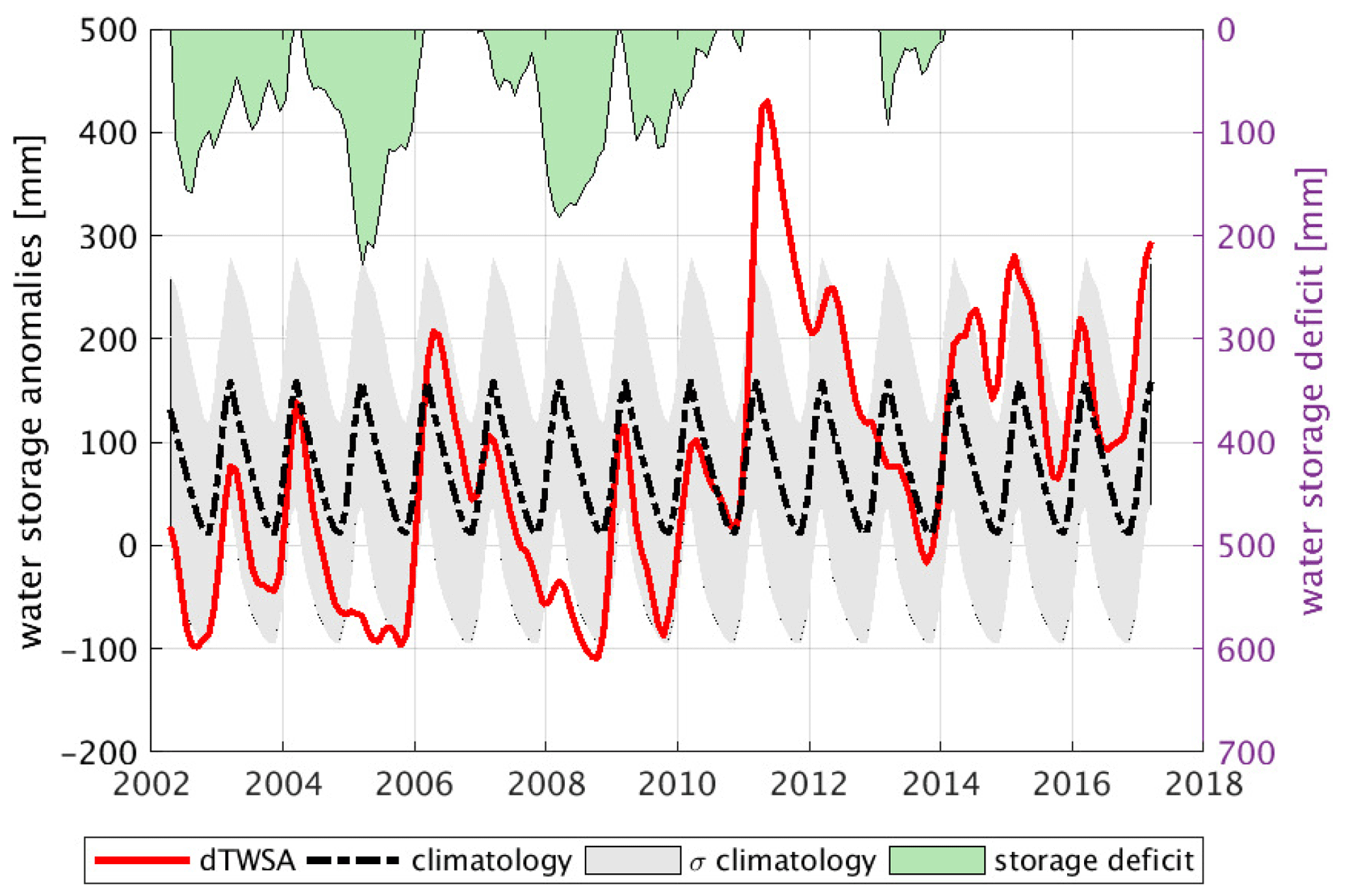
Figure 1Water storage deficit from GRACE. The smoothed and detrended TWSA (dTWSA – red plot) is reduced by its climatology (black plot) to estimate the deviation from the climatology. The negative residuals from the climatology are plotted on the upper axis as a green shaded area and scaled on the right side. The gray shading indicates ±1 SD (standard deviation) of the climatology.
3.2 Estimation of the required precipitation for storage deficit
The water balance equation, based on hydrological fluxes (Eq. 1), shows that the change in terrestrial water storage (dS) in a region for a given month (dt) depends on is the monthly precipitation (P; millimeters per month), evapotranspiration (ET; millimeters per month) and the streamflow (R, which includes both surface water and subsurface water; Swenson and Wahr, 2006). Assuming the relationship between precipitation and ET+R remains constant for a region, the variability in precipitation gives an idea of the possible variation in the storage. The amount of required precipitation needed to overcome a deficit can be estimated using the association between precipitation and the water storage anomaly (TWSA).
Monthly GPCP observations are first reduced by their mean for the April 2002–March 2017 period (i.e., the 15-year GRACE data record) to obtain the precipitation anomaly. Then, the relationship between precipitation and storage anomalies is derived. For this, first, both variables are smoothed by a 3-month moving average low-pass filter to remove high-frequency noise. Then, their linear trends are removed to reduce the impact of other processes, like groundwater, upstream abstraction, glacier melts, etc. (as discussed above), and to focus our analysis on subdecadal drought events within the GRACE period. The smoothed and detrended precipitation anomaly is then integrated in time to obtain the storage anomaly, which is termed the cumulative detrended smoothed precipitation anomaly (cdPA). Finally, the cdPA is compared with the smoothed and detrended storage anomaly (dTWSA).
An ecosystem may behave differently under stress (a deficit period) than under an excess water situation. In this study, the linear relationship between storage (dTWSA) and precipitation (cdPA) has been analyzed only during historical deficit periods as the system behaves differently under stress (Famiglietti et al., 1998; Vereecken et al., 2007). Several researchers used rainfall–runoff curves, like the Soil Conservation Service curve number (SCS-CN) for the computation of surface runoff, based on precipitation, with an assumption of a stable relation between rainfall and abstraction (Mishra et al., 2006; Singh et al., 2015; Verma et al., 2017). This study also assumes that the precipitation intensity for a region does not change significantly over time; consequently, the relationship between precipitation and storage variability can be considered stable.
Figure 2 shows the strength of this relationship with the correlation coefficients (Fig. 2a) and linear regression coefficients (Fig. 2b). Based on the linear relationship between dTWSA and cdPA, the required precipitation has been estimated. Regression coefficients greater than 1 means the required precipitation is more than the amount of missing water. This is because precipitation lost in other hydrological processes, like evapotranspiration and runoff (Eq. 1), is not observed by storage variability. A coefficient equal to 1 means the amount of required precipitation is the same as that storage loss, which means there is no other dominant process in the region. Coefficients less than 1 are the regions of weak precipitation–storage coupling, which can be due to other physical processes, like melting of snow/frozen surfaces, groundwater extraction, irrigation, etc. (non-red regions in Fig. 2a). Therefore, for most of the regions, the required precipitation is more than the amount of missing water (i.e., regression coefficients greater than 1), except for the regions with weak precipitation–storage coupling. For example, in higher latitudes, mass loss observed by GRACE during spring snowmelt is not directly linked to precipitation. Additionally, highly arid regions also have weak precipitation and storage signals. Therefore, the proposed method is not suitable for regions with weak precipitation–storage coupling. These regions of the weak association are identified based on regression coefficients below 1 (Fig. 2b), as less than 1, or a negative relationship between storage variability and precipitation, may describe a case in which storage variability is not linked to a direct precipitation effect. Also, locations with less than 5 months of drought in 15 years are considered as regions of the weak association because we do not have enough drought samples to derive their association. The regions of weak association (with regression coefficients less than 1) are considered as being unsuitable for the GRACE-based recovery analysis and have been masked out in this study.

Figure 2(a) Correlation coefficients and (b) regression coefficients between cumulative detrended precipitation anomalies (cdPA) and the detrended terrestrial water storage anomaly (dTWSA).
Based on the derived linear relationship between cdPA and dTWSA (Fig. 2b), a required precipitation is estimated for each regional drought period. The method for the estimation of required precipitation is shown in Fig. 3 at an example location (133.75∘ E, 16.75∘ S) in Australia. Figure 3a shows an agreement between cdPA (black plot) and dTWSA (red plot). In Fig. 3b, an absolute required precipitation (blue plot) is calculated, by adding precipitation climatology to the estimated surplus required precipitation (magenta plot), to fill the storage deficit (green plot). Analogous to an accounting methodology, this approach applies the assumption that generally more precipitation than usual (climatology) is required to replenish the losses incurred during drought. The example location has a strong annual signal (5–150 mm, with predominantly winter rain), which led to a relatively high ratio of required precipitation to the amount of missing water.
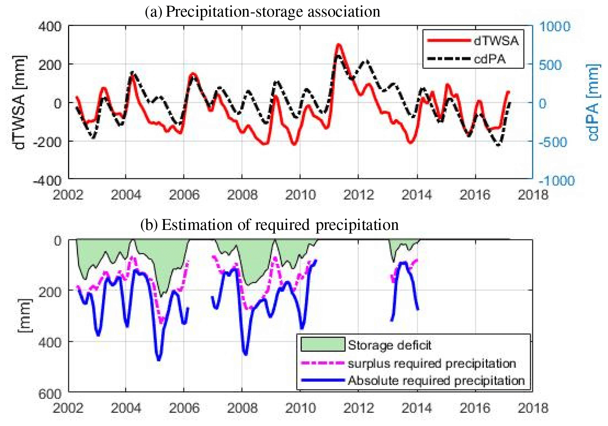
Figure 3Estimation of the required precipitation at an example location. (a) Cumulative detrended precipitation anomaly (cdPA) compared with the detrended storage anomaly (dTWSA). (b) Surplus required precipitation is estimated (magenta plot), from the linear relationship between dTWSA and cdPA, to fill the storage deficit (green plot). Then, precipitation climatology is added to obtain the absolute required precipitation (blue plot).
3.3 Historical precipitation analysis
Historical precipitation data from GPCP (1979 to 2017) are statistically analyzed, using signal decomposition, in order to create a simplistic precipitation forecast. Note that the motivation for providing a precipitation forecast here is not to present a state-of-the-art precipitation prediction but to demonstrate the potential utility of the terrestrial water storage deficit in determining required precipitation and estimating a likely time for recovery. This methodology could be augmented with any type of more complex precipitation forecasting approach.
3.3.1 Precipitation signal decomposition
Historical precipitation data are decomposed into a linear trend, inter-annual signal, annual/climatological cycle and the sub-seasonal components in order to explore temporal variability. First, a linear trend and an annual signal (mean of each month; e.g., all of January, February, etc.) are extracted from the original signal. Then, the residual signal is filtered by a 12-month low-pass window to split it into a smooth inter-annual signal and a high-frequency sub-seasonal signal. Together, the linear trend and inter-annual signal are considered to contribute to long-term variability. The individual variance of the annual, long-term and sub-seasonal signals is normalized by their sum in order to obtain their fractional contribution to local variability (Fig. 4). This provides an overview of the relative importance and spatial distribution of these components in global temporal variability. Figure 4 shows the fractional variance of the decomposed signal. For most regions, the annual signal dominates in precipitation (Fig. 4a). However, regions for which the wet season is not explicit in their climatology, a high-frequency signal plays a major role, for example in central Europe, eastern Siberia, western North America, southern Australia, etc. (Fig. 4c). Contrarily, the long-term signal obtained by combining linear trend and the inter-annual signal has the least variability globally (Fig. 4b). These smooth signals are driven by climate indices like the El Niño–Southern Oscillation (ENSO), Pacific Decadal Oscillation (PDO), and North Pacific Mode (NPM), etc. (Özger et al., 2009). The annual and long-term signals are directly applied for the signal reconstruction, with the assumption that a similar trend will continue.
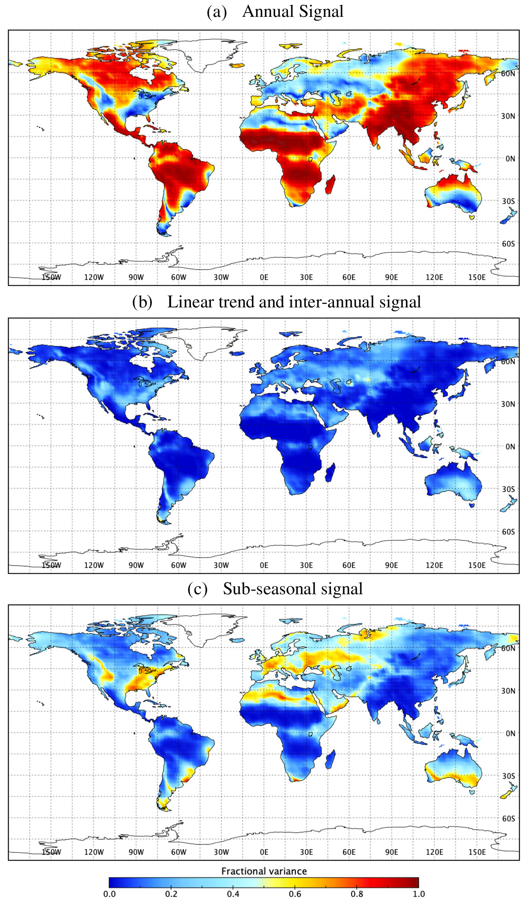
Figure 4Fractional variance in the decomposed signal to the full signal. (a) Annual signal, (b) long-term signal and (c) sub-seasonal high-frequency signal.
3.3.2 Signal reconstruction and forecasting skill
Based on the above findings, we formulate a statistical model for hindcasting precipitation. The annual signal and the linear trend extracted by signal decomposition (Sect. 3.3.1) are directly used for the precipitation reconstruction, with the assumption of the continuation of the similar variability. Furthermore, inter-annual variability in the precipitation data is added by autoregression for 10–14 months, depending on the duration of significant autocorrelation. Finally, the sub-seasonal signal is added, which is obtained from the residual of the inter-annual signal. This high-frequency signal has only 0–3 months of temporal autocorrelation; accordingly, we have limited skill in synthesizing the sub-seasonal signal.
Figure 5 shows the precipitation hindcast for January 2016–December 2017 at an example location (56.25∘ W, 27.75∘ S) in the La Plata basin. Figure 5a shows that the reconstructed precipitation (red plot), compared to its climatology (blue plot) and GPCP observations (black plot) for the same duration. Figure 5b shows the reconstructed inter-annual precipitation by autoregression. The figure shows that inter-annual autoregression (blue plot) signals have a good association with the observed inter-annual signal (black plot) for the first 11 months. The sub-seasonal autoregression is significant only for 2 months in the example location. The final hindcast is an integration of a linear trend, climatology, sub-seasonal and inter-annual autoregression.
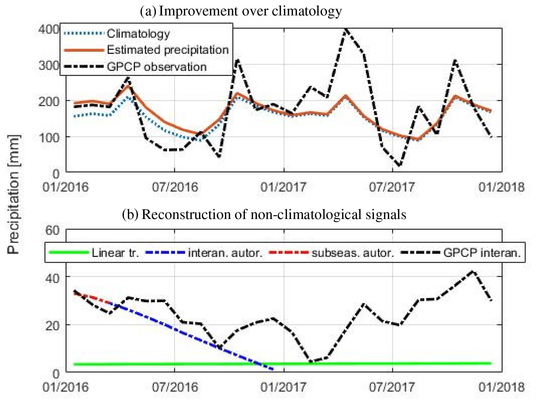
Figure 5Reconstruction of precipitation signal for 2016–2017. (a) The reconstructed signal compared with the GPCP observations and climatology. (b) The reconstruction of a long-term secular signal from the linear trend and inter-annual and sub-seasonal autoregression compared to GPCP inter-annual signal.
The precipitation reconstruction skill is used for a simplistic normal forecast. Furthermore, two additional precipitation scenarios are simulated by adding, respectively, 1 and 2 standard deviations (SDs) of precipitation to the normal forecast, which is used in probability recovery analysis.
3.4 Probabilistic recovery
Precipitation is the major control on drought dynamics. Knowing the amount of precipitation required to overcome a drought (at any instance and any location globally) presents the opportunity for the estimation of a likely drought recovery period. We can apply a probabilistic approach by using the historical precipitation forecast model to simulate different precipitation scenarios based on the historical distribution of precipitation for each region. Here, we propose three precipitation scenarios, namely (1) normal precipitation (as described in Sect. 3.3.2), (2) 1 standard deviation wetter than normal precipitation (assumed as being a wet month) and (3) 3 standard deviations wetter than normal precipitation (assumed as being an exceptionally wet month). The latter two scenarios are based on 1 standard deviation from the local precipitation climatology to simulate average rainy and extremely rainy months, respectively. Again, we assume that, in order to overcome a deficit due to drought, the ecosystem needs to receive a surplus of water that surpasses the climatological average. It follows that if drier than normal conditions were to persist indefinitely, then a drought could theoretically go on forever. The climatological average is integrated with the estimated surplus required precipitation (Fig. 3b; magenta plot) to obtain the absolute required precipitation (Fig. 3b; blue plot). Whenever precipitation is more than the absolute required precipitation, the system advances in recovery to its predrought state. Based on this hypothesis, we simulated the three scenarios for how long any instance of drought will continue, given the expected three precipitation cases. Note that the scenarios suggest the needed recovery time for normal, wet and exceptionally wet years, hence providing a minimum baseline for the duration of drought recovery.
4.1 Observed recovery time based on GRACE and GPCP observation
In this study, drought is defined by the negative deviation of TWSA from its record-length climatology. The observed recovery duration is measured directly from the storage deficit, as described previously (Fig. 1,; Thomas et al., 2014). For our approach, we need to know when the observed precipitation is more than the absolute required precipitation (Sect. 3.2). Figure 6 shows the recovery estimation of all the droughts that occurred during 2002–2017 at four random example locations, namely northwestern tropical Australia (123.25∘ E, 17.75∘ S), northeastern Argentina in the La Plata basin (56.25∘ W, 27.75∘ S), northern India in the Ganges Basin (78.75∘ E, 27.75∘ N) and northern Brazil in the Amazon basin (57.25∘ W, 2.25∘ S). Whenever the observed precipitation (Fig. 6; red plot; i.e., GPCP) is larger than the required precipitation (blue plot) for its respective month, the drought should end. Ideally, GRACE should also observe it simultaneously.
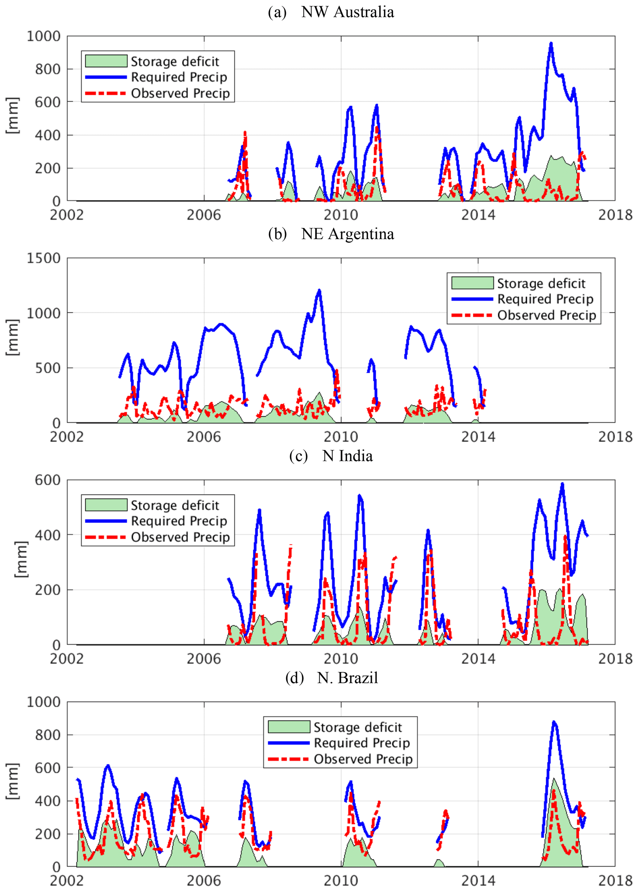
Figure 6Validation of the required precipitation estimate by drought recovery estimates at example locations. The different instances of drought show that drought ends (from the perspective of TWSA) whenever the observed precipitation (red plot) exceeds the required precipitation (blue plot).
The figure shows that the precipitation during a drought typically stays below its monthly required precipitation until the end of the drought. In most cases, precipitation crossed the required precipitation limit in precisely the same month when GRACE observed the end of the storage deficit. Even for the case of recurring droughts with 2 or more months' gap, both methods observed the end of the drought in approximately the same month. To examine our method in detail, we randomly selected a drought month and validated our approach and estimated the recovery time based on different precipitation scenarios in the following section.
4.2 Example of storage deficit and required precipitation
In this section, we discuss drought in an example month of January 2016. During the study period (2002–2017), the year 2015–2016 was the strongest El Niño on record, and many regions experienced drought. Nevertheless, this is done to demonstrate the recovery analysis and can be applied to any other time window. Figure 7 shows the regions under drought in January 2016 (Fig. 7a) and the estimated required precipitation to overcome the drought (Fig. 7b).
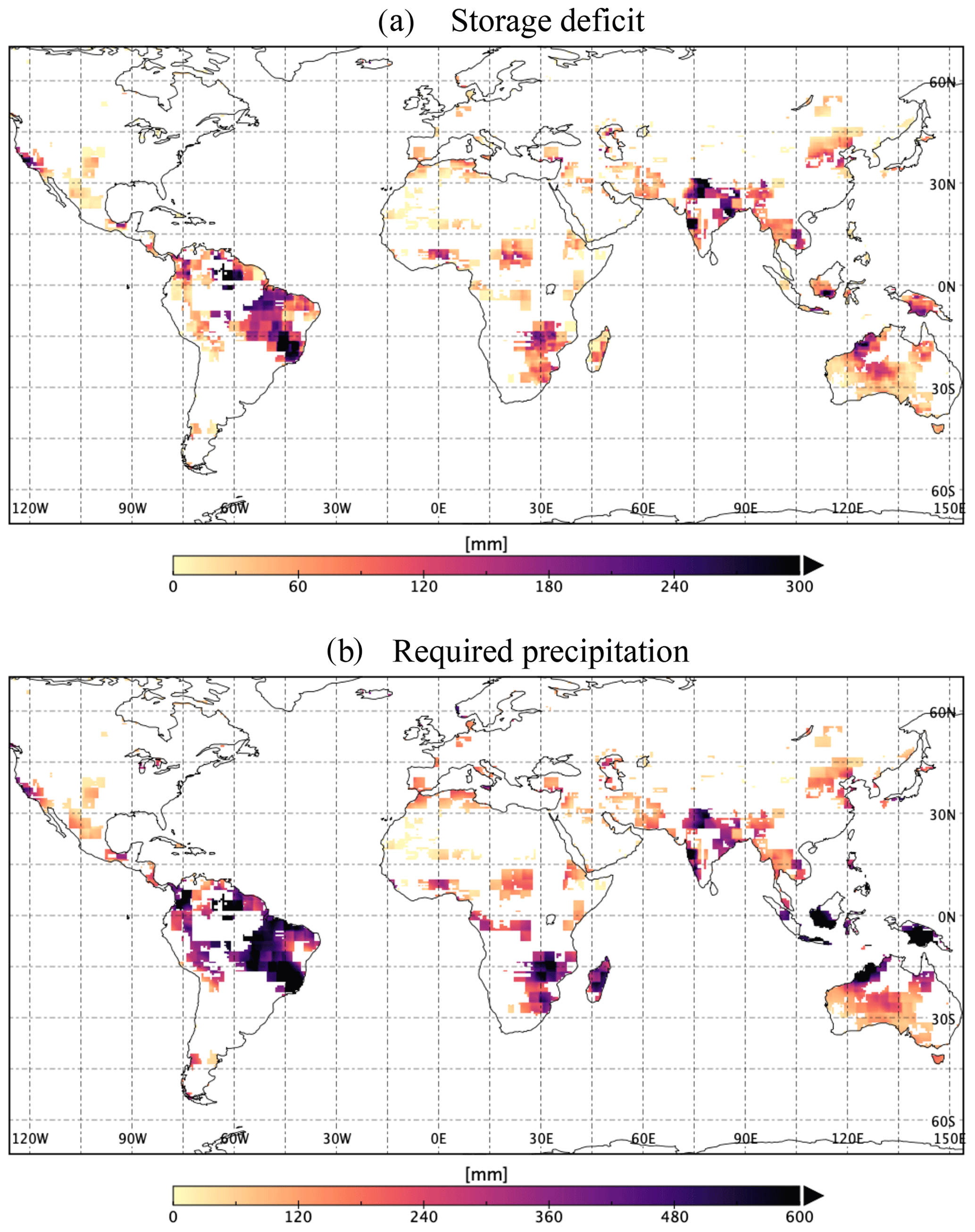
Figure 7(a) Storage deficit in an example month (January 2016). (b) The amount of required precipitation to fill the deficit.
Here, the severity of a drought is defined by the amount of water shortage in 1 month. All colors, other than white, in the figure are the drought-affected regions in January 2016, within the region of strong precipitation–storage relations (discussed in Sect. 3.2). The color bar demonstrates the severity of the drought, i.e., the amount of missing water (Fig. 7a) and the respective amount of required precipitation (Fig. 7b). Figure 7a shows that eastern Amazon, southern Australia, southeastern Africa and northern India were under severe drought in 2016 winter. For most of the region in the Southern Hemisphere, the amount of required precipitation is double the storage deficit because January is a summer month and water demand is higher.
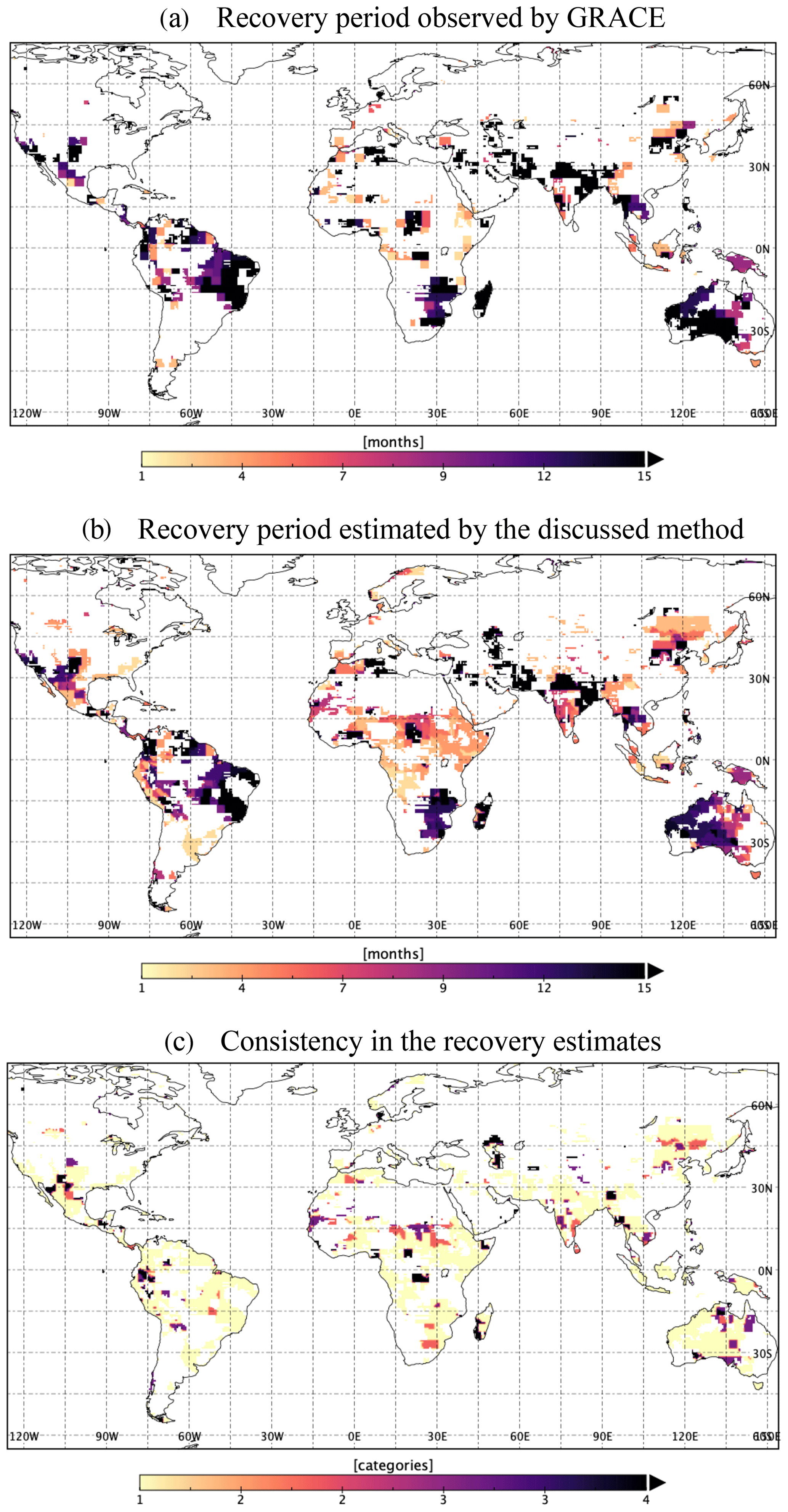
Figure 8Validation of the estimated required precipitation by the recovery duration from the January 2016 drought observed from (a) GRACE and (b) estimated, by the discussed method, using GRACE and GPCP observations. (c) Consistency in the observed recovery duration by GRACE and GPCP (1=1–2 months' difference, 2=3–4 months' difference, 3=5–8 months' difference and months' difference).
4.2.1 Validation
To validate our approach, we compared recovery periods in Fig. 8. The figure shows the recovery period from the January 2016 drought state, observed by GRACE (Fig. 8a), and estimated recovery based on absolute required precipitation and GPCP observations (Fig. 8b). Figure 8c highlights the consistency in the estimated recovery period, where 1 indicates a 1–2 months' difference, 2 indicates 3–4 months' difference, 3 indicates 5–8 months' difference and 4 indicates 9+ months' difference. The black area in Fig. 8c is the region with extremely different recovery estimates. The difference between the estimated recovery periods can be partially attributed to the spatial resolution of the two data sets and uncertainties in the data sets. Though GRACE 3∘ mascon and GPCP 2.5∘ are considered comparable, areas of the unit representations are, nevertheless, different at different locations like at the Equator (≈10 000 km2) and close to the poles (80 000 km2). However, as drought is a smooth process, the impact of neighboring pixels should not affect the analysis significantly. For the January 2016 drought, approximately 80 % of the masked global land area demonstrated a similar recovery period (±1–2 months) to what was predicted (category 1 in Fig. 8c).
4.2.2 Precipitation scenarios
This section demonstrates the probability of the recovery duration in different precipitation scenarios. In the first section, we discussed the expected recovery percentage within 1 month in three different precipitation scenarios. And in the second section, we projected the duration needed to overcome the January 2016 drought within the study period (until March 2017).
The expected 1-month recovery state
Spatiotemporal patterns of drought at the global scale are largely uncharacterized. Often, 1 month of surplus precipitation is not enough to fill the entire deficit. However, if rain is significantly above average immediately after/during the drought, the recovery time decreases dramatically. We simulated a 1-month (February 2016) recovery percentage for the January 2016 drought, given the three different precipitation scenarios (discussed in Sect. 3.4). The surplus precipitation within 1 month (February) is divided by the required reconstructed precipitation to calculate the percentage recovery. In most of the drought-affected regions, the recovery percentage of our forecasted normal precipitation (Sect. 3.3.2) for February 2016 is more than the recovery percentage of observed GPCP precipitation (Fig. 9d). This indicates that February 2016 was drier than our estimated normal. Most of the region recovered in an extremely wet scenario (Fig. 9c) within 1 month, except for regions dominated by summer monsoons (Fig. 9c; orange/yellow area), which had less than 30 % recovery, as February is not a rainy season for this region. This shows a case in which regions with high-amplitude seasonal cycles in precipitation mostly recover during their rainy season, which varies globally.
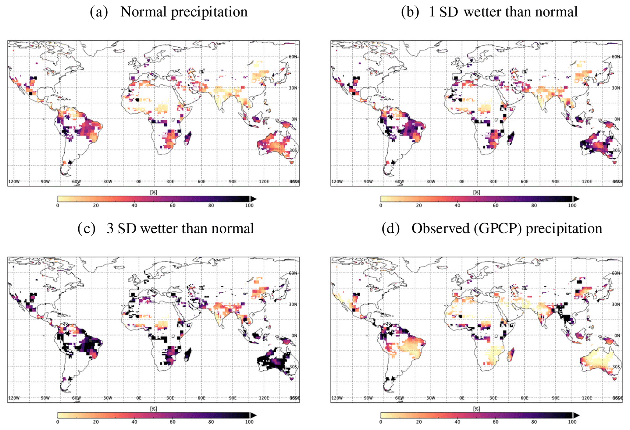
Figure 9Expected percent recovery in 1 month, given the three different precipitation scenarios and the observed GPCP precipitation.
Best estimated time for recovery
Recovery time varies from immediate (i.e., 1 month) to several years across different climate zones and depends on the severity of the drought. Figure 10 shows the predicted recovery duration of the January 2016 drought state, which ranges from 1 month (yellow) to not recoverable within the study period of 15 months (black). Figure 10d shows the recovery duration observed by GRACE, which is considered as being the truth. Figure 10a and b show that most of the region under severe drought in 2016 did not recover with even 1 standard deviation of wetter than normal precipitation, and the drought in this region continued beyond a year. In the extremely wetter (3 standard deviations) than normal situation (Fig. 10c), most of the regions recovered within 4–5 months, except for regions of the most severe drought, such as the southeastern Amazon and southern Africa. Even in the extremely wet scenario, the monsoon regions (Fig. 10c) recovered only during their rainy season (6–7 months after January 2016). This demonstrates that information on the state of precipitation, compared to its usual levels, can provide an idea of the expected drought recovery duration, provided we know the amount of precipitation required.
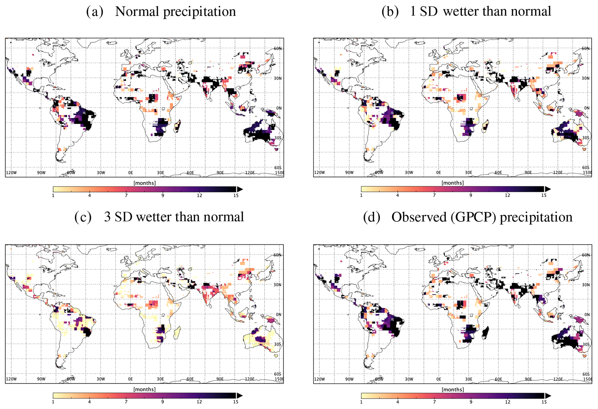
Figure 10Duration of drought recovery from January 2016, given the three different precipitation scenarios, as observed by GRACE.
Here we define drought intensity and duration using the observed storage deficit from GRACE TWSA, which is a 3-month or greater negative deviation from the historical, record-length climatology for each region, following Thomas et al. (2014). Generally, we considered this to be a better metric of integrated drought effects than a negative departure from climatology in precipitation or soil moisture because the former includes all components of the water cycle and represents the integrated state of the local water budget closure, dS∕dt. We observe that, occasionally, precipitation anomalies are depressed a couple of months before GRACE sees the beginning of the drought onset because the net water mass balance can stay stable for some time by a compensating decrease in ET and runoff. Similarly, precipitation shows a positive deviation from climatology (i.e., excess precipitation) well before GRACE observes the end of the drought because of the time lag in filling the root zone soil moisture (Eltahir and Yeh, 1999). Dettinger (2013) and Maxwell et al. (2013) also argued that drought onset is quicker than drought termination. Sometimes very heavy rain can quickly bring a region entirely out of a drought, but in many cases, continuous surplus precipitation is needed to bring the entire water column (i.e., from the surface to groundwater) to full recovery.
The critical feature of the GRACE-based drought recovery framework is the estimation of required precipitation to fill a storage deficit. Figure 2 shows that TWSA is closely associated with a cumulative precipitation anomaly for most regions, except in deserts and high latitudes. In large arid regions, monthly storage variability is significantly low due to low rainfall. In high latitudes, seasonal water storage variability is mainly driven by temperature because of snow accumulation and melt. Typically, in cold regions, winter snow accumulation and spring snowmelt drive increases and declines in TWSA, decoupling the storage variability from precipitation variability, which leads to a phase shift in their seasonality and a weak correlation between them (Reager and Famiglietti, 2013). For these reasons, a storage-based drought recovery metric is not as capable in desert and high-latitude areas and is masked out in the results section.
Variability in the historical precipitation data is analyzed by signal decomposition to develop a simple precipitation forecast model. Precipitation signals are hindcast by combining the climatology with the linear trend and an inter-annual signal estimated from autoregression. Figure 4 shows that, in most regions, seasonal variability is the strongest signal, except in big deserts, Eurasia and northwest America. These regions have high sub-seasonal variability in precipitation, which is hard to reconstruct. Additionally, due to the contribution of snowfall in higher latitudes and very low rainfall in deserts, bias correction in precipitation data is relatively less reliable. Consequently, we have less confidence in precipitation simulations in those regions.
In addition to the normal precipitation forecast, two more precipitation scenarios are simulated based on 1 and 3 standard deviations from the climatology, assuming that a system recovers from drought only when the precipitation is more than the usual (climatological) precipitation of the corresponding month. Figure 9 demonstrates the percentage recovery, given these three different precipitation scenarios. The figure shows that most regions show significant recovery within 1 month in 3 standard deviations wetter than the normal scenario, except for regions which are not in their respective rainy season. As precipitation can be scarce in non-rainy-season months, even 3 standard deviations wetter than the historical average precipitation would not be a substantial amount of rain to replenish the water deficit in these periods. We further investigate the recovery duration based on different precipitation scenarios (Fig. 10) and find that, under normal precipitation, most regions will not recover significantly within the study duration, but for 3 standard deviations, i.e., wetter than normal rain, they recover within 3–4 months. However, for the regions with a strong seasonal intensity of precipitation (monsoonal region), the figure showed recovery only during its rainy season (after 6–7 months) even in the extremely wet scenario.
We validated our required precipitation estimates by comparing the recovery period observed by GRACE and estimated by our method on the GPCP observations (Fig. 7) at different locations, which showed good concurrence. Also in Fig. 10, the drought recovery duration for an example month of January 2016 demonstrated a good agreement between the observed recovery by GRACE and estimated recovery by GPCP for most of the masked regions (80 % within ±1 month).
Knowing the present state of precipitation, i.e., how much surplus we have over the usual climatology of a region, can give an idea of the expected recovery duration, provided we know the amount of precipitation needed to fill the deficit. With improved precipitation forecasting skills, more accurate drought recovery estimates can be obtained. Nevertheless, the study demonstrates a case of the application of GRACE for the estimation of required precipitation for drought recovery.
Increasing water demand and future uncertainties in climate necessitate the assessment of the potential impact of drought and its expected recovery duration. The consequences of drought can be minimized through adaptation and risk management efforts, which are informed by the amount of missing water in a system and the required precipitation needed to bring it back to normal (as shown in Fig. 7). Recurring droughts due to insufficient recovery can be minimized, to a large extent, by managing water resources wisely – particularly during the deficit period – until all of the hydrological components revert to the predrought state. The study demonstrates the utility of GRACE terrestrial water storage anomalies (TWSA) in obtaining statistics of hydrological drought, i.e., its recovery period and the precipitation required to recover, with a sensitivity test, to different precipitation scenarios. The benefits of the GRACE-based drought index for drought analysis are (1) the independency from meteorological variables, unlike other drought indices (PDSI, SPEI and SPI), and (2) the spatial coverage of the GRACE data (much of the globe). However, recovery analysis is limited to the areas in which linear relationships between TWSA and cumulative precipitation anomaly exhibit strong linkages. The findings of this study are (1) the GRACE-based drought index is valid for estimating the required precipitation for drought recovery, and (2) the period of drought recovery depends on the intensity of precipitation i.e., in the dry season of the year drought continues even with above-normal precipitation. The recovery period estimated by our approach matches well with the recovery observed by GRACE for most of the masked regions (80 %) for the demonstrated drought month. This approach can be extended with the availability of the new GRACE follow-on (GRACE-FO) data sets launched in May 2018. The proposed method and analyses in this study are applicable for the development of an operational drought monitoring system that can provide actionable information for drought recovery, given that skillful precipitation prediction is available.
The study used GRACE mascon (RL06) solutions from the Jet Propulsion Laboratory (JPL), available at https://grace.jpl.nasa.gov (last access: 3 March 2019; NASA, 2019), and GPCP V2.3, available at https://www.esrl.noaa.gov/psd/ (last access: 20 May 2019; NOAA, 2019).
The supplement related to this article is available online at: https://doi.org/10.5194/hess-25-511-2021-supplement.
AS contributed to the data curation, formal analysis, writing and visualization. JTR conceptualized, supervised and acquired funding to conduct this study. JTR also helped in writing and editing the text. AB also contributed through supervision and funding acquisition.
The authors declare that they have no conflict of interest.
The research was carried out at the Jet Propulsion Laboratory, California Institute of Technology, under a contract with the National Aeronautics and Space Administration.
This research has been supported by the GRACE Science team.
This paper was edited by Patricia Saco and reviewed by three anonymous referees.
Adler, R. F., Huffman, G. J., Chang, A., Ferraro, R., Xie, P.-P., Janowiak, J., Rudolf, B., Schneider, U., Curtis, S., Bolvin, D., Gruber, A., Susskind, J., Arkin, P., and Nelkin, E.: The Version-2 Global Precipitation Climatology Project (GPCP) Monthly Precipitation Analysis (1979–Present), J. Hydrometeorol., 4, 1147–1167, https://doi.org/10.1175/1525-7541(2003)004<1147:TVGPCP>2.0.CO;2, 2003.
Awange, J. L., Khandu, Schumacher, M., Forootan, E., and Heck, B.: Exploring hydro-meteorological drought patterns over the Greater Horn of Africa (1979–2014) using remote sensing and reanalysis products, Adv. Water Resour., 94, 45–59, https://doi.org/10.1016/j.advwatres.2016.04.005, 2016.
Behrangi, A., Nguyen, H., and Granger, S.: Probabilistic Seasonal Prediction of Meteorological Drought Using the Bootstrap and Multivariate Information, J. Appl. Meteorol. Clim., 54, 1510–1522, https://doi.org/10.1175/JAMC-D-14-0162.1, 2015.
Behrangi, A., Gardner, A., Reager, J. T., Fisher, J. B., Yang, D., Huffman, G. J., and Adler, R. F.: Using GRACE to Estitmate Snowfall Accumulation and Assess Gauge Undercatch Corrections in High Latitudes, J. Climate, 31, 8689–8704, https://doi.org/10.1175/JCLI-D-18-0163.1, 2018.
Chen, J. L., Wilson, C. R., Tapley, B. D., Yang, Z. L., and Niu, G. Y.: 2005 drought event in the Amazon River basin as measured by GRACE and estimated by climate models, J. Geophys. Res., 114, B05404, https://doi.org/10.1029/2008JB006056, 2009.
Cook, B. I., Smerdon, J. E., Seager, R., and Coats, S.: Global warming and 21st century drying, Clim. Dynam., 43, 2607–2627, https://doi.org/10.1007/s00382-014-2075-y, 2014.
Cook, B. I., Mankin, J. S., and Anchukaitis, K. J.: Climate Change and Drought: From Past to Future, Curr. Clim. Change Rep., 4, 164–179, https://doi.org/10.1007/s40641-018-0093-2, 2018.
Dettinger, M. D.: Atmospheric Rivers as Drought Busters on the U.S. West Coast, J. Hydrometeorol., 14, 1721–1732, https://doi.org/10.1175/JHM-D-13-02.1, 2013.
Eicker, A., Forootan, E., Springer, A., Longuevergne, L., and Kusche, J.: Does GRACE see the terrestrial water cycle “intensifying”?, J. Geophys. Res.-Atmos., 121, 733–745, https://doi.org/10.1002/2015JD023808, 2016.
Eltahir, E. A. B. and Yeh, P. J.-F.: On the asymmetric response of aquifer water level to floods and droughts in Illinois, Water Resour. Res., 35, 1199–1217, https://doi.org/10.1029/1998WR900071, 1999.
Famiglietti, J. S., Rudnicki, J. W., and Rodell, M.: Variability in surface moisture content along a hillslope transect: Rattlesnake Hill, Texas, J. Hydrol., 210, 259–281, https://doi.org/10.1016/S0022-1694(98)00187-5, 1998.
Fasullo, J. T., Lawrence, D. M., and Swenson, S. C.: Are GRACE-era Terrestrial Water Trends Driven by Anthropogenic Climate Change?, Adv. Meteorol., 2016, e4830603, https://doi.org/10.1155/2016/4830603, 2016.
Forootan, E., Khaki, M., Schumacher, M., Wulfmeyer, V., Mehrnegar, N., van Dijk, A. I. J. M., Brocca, L., Farzaneh, S., Akinluyi, F., Ramillien, G., Shum, C. K., Awange, J., and Mostafaie, A.: Understanding the global hydrological droughts of 2003–2016 and their relationships with teleconnections, Sci. Total Environ., 650, 2587–2604, https://doi.org/10.1016/j.scitotenv.2018.09.231, 2019.
Frappart, F., Papa, F., Santos da Silva, J., Ramillien, G., Prigent, C., Seyler, F., and Calmant, S.: Surface freshwater storage and dynamics in the Amazon basin during the 2005 exceptional drought, Environ. Res. Lett., 7, 044010, https://doi.org/10.1088/1748-9326/7/4/044010, 2012.
Gerdener, H., Engels, O., and Kusche, J.: A framework for deriving drought indicators from the Gravity Recovery and Climate Experiment (GRACE), Hydrol. Earth Syst. Sci., 24, 227–248, https://doi.org/10.5194/hess-24-227-2020, 2020.
Guevara-Murua, A., Williams, C. A., Hendy, E. J., and Imbach, P.: 300 years of hydrological records and societal responses to droughts and floods on the Pacific coast of Central America, Clim. Past, 14, 175–191, https://doi.org/10.5194/cp-14-175-2018, 2018.
Hao, Z., Singh, V. P., and Xia, Y.: Seasonal Drought Prediction: Advances, Challenges, and Future Prospects, Rev. Geophys., 56, 108–141, https://doi.org/10.1002/2016RG000549, 2018.
Houborg, R., Rodell, M., Li, B., Reichle, R., and Zaitchik, B. F.: Drought indicators based on model-assimilated Gravity Recovery and Climate Experiment (GRACE) terrestrial water storage observations: GRACE-Based Drought Indicators, Water Resour. Res., 48, W07525, https://doi.org/10.1029/2011WR011291, 2012.
Keshavarz, M. R., Vazifedoust, M., and Alizadeh, A.: Drought monitoring using a Soil Wetness Deficit Index (SWDI) derived from MODIS satellite data, Agr. Water Manage., 132, 37–45, https://doi.org/10.1016/j.agwat.2013.10.004, 2014.
Keys, R.: Cubic convolution interpolation for digital image processing, IEEE Trans. Acoust. Speech Signal Process., 29, 1153–1160, https://doi.org/10.1109/TASSP.1981.1163711, 1981.
Li, B., Rodell, M., Kumar, S., Beaudoing, H. K., Getirana, A., Zaitchik, B. F., de Goncalves, L. G. , Cossetin, C., Bhanja, S., Mukherjee, A., Tian, S., Tangdamrongsub, N., Long, D., Nanteza, J., Lee, J., Policelli, F., Goni, I. B., Daira, D., Bila, M., de Lannoy, G., Mocko, D., Steele-Dunne, S. C., Save, H., and Bettadpur, S.: Global GRACE Data Assimilation for Groundwater and Drought Monitoring: Advances and Challenges, Water Resour. Res., 55, 7564–7586, https://doi.org/10.1029/2018WR024618, 2019.
Long, D., Scanlon, B. R., Longuevergne, L., Sun, A. Y., Fernando, D. N., and Save, H.: GRACE satellite monitoring of large depletion in water storage in response to the 2011 drought in Texas: GRACE-Based Drought Monitoring, Geophys. Res. Lett., 40, 3395–3401, https://doi.org/10.1002/grl.50655, 2013.
Lyon, B. and DeWitt, D. G.: A recent and abrupt decline in the East African long rains, Geophys. Res. Lett., 39, L02702, https://doi.org/10.1029/2011GL050337, 2012.
Maity, R., Suman, M., and Verma, N. K.: Drought prediction using a wavelet based approach to model the temporal consequences of different types of droughts, J. Hydrol., 539, 417–428, https://doi.org/10.1016/j.jhydrol.2016.05.042, 2016.
Martínez-Fernández, J., González-Zamora, A., Sánchez, N., and Gumuzzio, A.: A soil water based index as a suitable agricultural drought indicator, J. Hydrol., 522, 265–273, https://doi.org/10.1016/j.jhydrol.2014.12.051, 2015.
Maxwell, J. T., Ortegren, J. T., Knapp, P. A., and Soulé, P. T.: Tropical Cyclones and Drought Amelioration in the Gulf and Southeastern Coastal United States, J. Climate, 26, 8440–8452, https://doi.org/10.1175/JCLI-D-12-00824.1, 2013.
McKee, T. B., Doesken, N. J., and Kleist, J.: The relationship of drought frequency and duration to time scales, in: Eighth Conference on Applied Climatology, 17–22 January 1993, Anaheim, California, 179–184, 1993.
Mishra, A. K. and Singh, V. P.: A review of drought concepts, J. Hydrol., 391, 202–216, https://doi.org/10.1016/j.jhydrol.2010.07.012, 2010.
Mishra, S. K., Sahu, R. K., Eldho, T. I., and Jain, M. K.: A generalized relation between initial abstraction and potential maximum retention in SCS-CN-based model, Int. J. River Basin Manage., 4, 245–253, https://doi.org/10.1080/15715124.2006.9635294, 2006.
Mo, K. C.: Drought onset and recovery over the United States, J. Geophys. Res.-Atmos., 116, D20106, https://doi.org/10.1029/2011JD016168, 2011.
NASA: Measuring Earth's Surface Mass and Water Changes, available at: https://grace.jpl.nasa.gov/, last access: 3 March 2019.
NOAA: Physical Sciences Laboratory, available at: https://psl.noaa.gov/, last access: 20 May 2019.
Otkin, J. A., Anderson, M. C., Hain, C., Mladenova, I. E., Basara, J. B., and Svoboda, M.: Examining Rapid Onset Drought Development Using the Thermal Infrared-Based Evaporative Stress Index, J. Hydrometeorol., 14, 1057–1074, https://doi.org/10.1175/JHM-D-12-0144.1, 2013.
Otkin, J. A., Anderson, M. C., Hain, C., and Svoboda, M.: Using Temporal Changes in Drought Indices to Generate Probabilistic Drought Intensification Forecasts, J. Hydrometeorol., 16, 88–105, https://doi.org/10.1175/JHM-D-14-0064.1, 2015.
Özger, M., Mishra, A. K., and Singh, V. P.: Low frequency drought variability associated with climate indices, J. Hydrol., 364, 152–162, https://doi.org/10.1016/j.jhydrol.2008.10.018, 2009.
Palmer, W. C.: Meteorological Drought, Research Paper No. 45, US Department of Commerce Weather Bureau, Washington, D.C., available at: https://www.ncdc.noaa.gov/temp-and-precip/drought/docs/palmer.pdf (last access: 11 January 2018), 1965.
Pan, M., Yuan, X., and Wood, E. F.: A probabilistic framework for assessing drought recovery, Geophys. Res. Lett., 40, 3637–3642, https://doi.org/10.1002/grl.50728, 2013.
Reager, J. T. and Famiglietti, J. S.: Characteristic mega-basin water storage behavior using GRACE, Water Resour. Res., 49, 3314–3329, https://doi.org/10.1002/wrcr.20264, 2013.
Schwalm, C. R., Anderegg, W. R. L., Michalak, A. M., Fisher, J. B., Biondi, F., Koch, G., Litvak, M., Ogle, K., Shaw, J. D., Wolf, A., Huntzinger, D. N., Schaefer, K., Cook, R., Wei, Y., Fang, Y., Hayes, D., Huang, M., Jain, A., and Tian, H.: Global patterns of drought recovery, Nature, 548, 202–205, https://doi.org/10.1038/nature23021, 2017.
Seager, R., Nakamura, J., and Ting, M.: Mechanisms of Seasonal Soil Moisture Drought Onset and Termination in the Southern Great Plains, J. Hydrometeorol., 20, 751–771, https://doi.org/10.1175/JHM-D-18-0191.1, 2019.
Singh, A., Behrangi, A., Fisher, J. B., and Reager, J. T.: On the Desiccation of the South Aral Sea Observed from Spaceborne Missions, Remote Sens., 10, 793, https://doi.org/10.3390/rs10050793, 2018.
Singh, P. K., Mishra, S. K., Berndtsson, R., Jain, M. K., and Pandey, R. P.: Development of a Modified SMA Based MSCS-CN Model for Runoff Estimation, Water Resour. Manage., 29, 4111–4127, https://doi.org/10.1007/s11269-015-1048-1, 2015.
Springer, A., Eicker, A., Bettge, A., Kusche, J., and Hense, A.: Evaluation of the Water Cycle in the European COSMO-REA6 Reanalysis Using GRACE, Water, 9, 289, https://doi.org/10.3390/w9040289, 2017.
Sridhar, V., Hubbard, K. G., You, J., and Hunt, E. D.: Development of the Soil Moisture Index to Quantify Agricultural Drought and Its “User Friendliness” in Severity-Area-Duration Assessment, J. Hydrometeorol., 9, 660–676, https://doi.org/10.1175/2007JHM892.1, 2008.
Sun, A. Y., Scanlon, B. R., AghaKouchak, A., and Zhang, Z.: Using GRACE Satellite Gravimetry for Assessing Large-Scale Hydrologic Extremes, Remote Sens., 9, 1287, https://doi.org/10.3390/rs9121287, 2017.
Swenson, S. and Wahr, J.: Estimating Large-Scale Precipitation Minus Evapotranspiration from GRACE Satellite Gravity Measurements, J. Hydrometeorol., 7, 252–270, https://doi.org/10.1175/JHM478.1, 2006.
Thomas, A. C., Reager, J. T., Famiglietti, J. S., and Rodell, M.: A GRACE-based water storage deficit approach for hydrological drought characterization, Geophys. Res. Lett., 41, 1537–1545, https://doi.org/10.1002/2014GL059323, 2014.
Vereecken, H., Kamai, T., Harter, T., Kasteel, R., Hopmans, J., and Vanderborght, J.: Explaining soil moisture variability as a function of mean soil moisture: A stochastic unsaturated flow perspective, Geophys. Res. Lett., 34, L22402, https://doi.org/10.1029/2007GL031813, 2007.
Verma, S., Mishra, S. K., Singh, A., Singh, P. K., and Verma, R. K.: An enhanced SMA based SCS-CN inspired model for watershed runoff prediction, Environ. Earth Sci., 76, 736, https://doi.org/10.1007/s12665-017-7062-2, 2017.
Vicente-Serrano, S. M., Beguería, S., and López-Moreno, J. I.: A Multiscalar Drought Index Sensitive to Global Warming: The Standardized Precipitation Evapotranspiration Index, J. Climate, 23, 1696–1718, https://doi.org/10.1175/2009JCLI2909.1, 2009.
Watkins, M. M., Wiese, D. N., Yuan, D.-N., Boening, C., and Landerer, F. W.: Improved methods for observing Earth's time variable mass distribution with GRACE using spherical cap mascons, J. Geophys. Res.-Solid, 120, 2648–2671, https://doi.org/10.1002/2014JB011547, 2015.
Wiese, D. N., Landerer, F. W., and Watkins, M. M.: Quantifying and reducing leakage errors in the JPL RL05M GRACE mascon solution, Water Resour. Res., 52, 7490–7502, https://doi.org/10.1002/2016WR019344, 2016.
Wiese, D. N., Yuan, D.-N., Boening, C., Landerer, F. W., and Watkins, M. M.: JPL GRACE Mascon Ocean, Ice, and Hydrology Equivalent Water Height Release 06 Coastal Resolution Improvement (CRI) Filtered Version 1.0, Dataset, PO.DAAC, CA, USA, https://doi.org/10.5067/TEMSC-3MJC6, 2018.
Wilhite, D. A. and Glantz, M. H.: Understanding: the Drought Phenomenon: The Role of Definitions, Water Int., 10, 111–120, https://doi.org/10.1080/02508068508686328, 1985.
Yirdaw, S. Z., Snelgrove, K. R., and Agboma, C. O.: GRACE satellite observations of terrestrial moisture changes for drought characterization in the Canadian Prairie, J. Hydrol., 356, 84–92, https://doi.org/10.1016/j.jhydrol.2008.04.004, 2008.
Yuan, X., Wood, E. F., Chaney, N. W., Sheffield, J., Kam, J., Liang, M., and Guan, K.: Probabilistic Seasonal Forecasting of African Drought by Dynamical Models, J. Hydrometeorol., 14, 1706–1720, https://doi.org/10.1175/JHM-D-13-054.1, 2013.
Zhang, D., Zhang, Q., Werner, A. D., and Liu, X.: GRACE-Based Hydrological Drought Evaluation of the Yangtze River Basin, China, J. Hydrometeorol., 17, 811–828, https://doi.org/10.1175/JHM-D-15-0084.1, 2015.
Zhao, C., Huang, Y., Li, Z., and Chen, M.: Drought Monitoring of Southwestern China Using Insufficient GRACE Data for the Long-Term Mean Reference Frame under Global Change, J. Climate, 31, 6897–6911, https://doi.org/10.1175/JCLI-D-17-0869.1, 2018.
Zhao, M. A. G., Velicogna, I., and Kimball, J. S.: A Global Gridded Dataset of GRACE Drought Severity Index for 2002–14: Comparison with PDSI and SPEI and a Case Study of the Australia Millennium Drought, J. Hydrometeorol., 18, 2117–2129, https://doi.org/10.1175/JHM-D-16-0182.1, 2017.