the Creative Commons Attribution 4.0 License.
the Creative Commons Attribution 4.0 License.
 | 22 Sep 2021
A comparison of tools and techniques for stabilising unmanned aerial system (UAS) imagery for surface flow observations
Robert Ljubičić
Dariia Strelnikova
Matthew T. Perks
Anette Eltner
Salvador Peña-Haro
Alonso Pizarro
Silvano Fortunato Dal Sasso
Ulf Scherling
Pietro Vuono
Salvatore Manfreda
While the availability and affordability of unmanned aerial systems (UASs) has led to the rapid development of remote sensing applications in hydrology and hydrometry, uncertainties related to such measurements must be quantified and mitigated. The physical instability of the UAS platform inevitably induces motion in the acquired videos and can have a significant impact on the accuracy of camera-based measurements, such as velocimetry. A common practice in data preprocessing is compensation of platform-induced motion by means of digital image stabilisation (DIS) methods, which use the visual information from the captured videos – in the form of static features – to first estimate and then compensate for such motion. Most existing stabilisation approaches rely either on customised tools developed in-house, based on different algorithms, or on general purpose commercial software. Intercomparison of different stabilisation tools for UAS remote sensing purposes that could serve as a basis for selecting a particular tool in given conditions has not been found in the literature. In this paper, we have attempted to summarise and describe several freely available DIS tools applicable to UAS velocimetry. A total of seven tools – six aimed specifically at velocimetry and one general purpose software – were investigated in terms of their (1) stabilisation accuracy in various conditions, (2) robustness, (3) computational complexity, and (4) user experience, using three case study videos with different flight and ground conditions. In an attempt to adequately quantify the accuracy of the stabilisation using different tools, we have also presented a comparison metric based on root mean squared differences (RMSDs) of inter-frame pixel intensities for selected static features. The most apparent differences between the investigated tools have been found with regards to the method for identifying static features in videos, i.e. manual selection of features or automatic. State-of-the-art methods which rely on automatic selection of features require fewer user-provided parameters and are able to select a significantly higher number of potentially static features (by several orders of magnitude) when compared to the methods which require manual identification of such features. This allows the former to achieve a higher stabilisation accuracy, but manual feature selection methods have demonstrated lower computational complexity and better robustness in complex field conditions. While this paper does not intend to identify the optimal stabilisation tool for UAS-based velocimetry purposes, it does aim to shed light on details of implementation, which can help engineers and researchers choose the tool suitable for their needs and specific field conditions. Additionally, the RMSD comparison metric presented in this paper can be used in order to measure the velocity estimation uncertainty induced by UAS motion.
- Article
(10997 KB) - Full-text XML
-
Supplement
(24506 KB) - BibTeX
- EndNote


The application of unmanned aerial systems (UASs; often referred to as unmanned or uncrewed aerial vehicles, UAVs, or remotely piloted aircraft systems, RPAS) for large-scale image velocimetry is expanding rapidly due to several key factors, namely (1) the reduction in UAS production costs, (2) technological advances in digital photography and videography, and (3) development and improvement of various velocimetry methods (Manfreda et al., 2018, 2019; Pearce et al., 2020). To perform an adequate velocimetry analysis using UAS video data, the relationship between the real-world coordinates and the points in the video's region of interest (ROI) should be constant throughout the entire video frame sequence. These conditions are not practically attainable using UAS, even with a camera gimbal, given the current state of UAS technology. This is because even small camera movement during high-altitude flights, caused by vibrations of the UAS, wind-induced turbulence, issues with GPS positioning, and operator inexperience, can result in large apparent displacements of features in the ROI. Similar issues can arise from videos obtained using handheld devices and even from terrestrial cameras (Le Boursicaud et al., 2016). To reduce motion-induced errors, it is necessary to perform stabilisation of the UAS-acquired video onto a fixed frame of reference prior to the velocimetry analysis.
Image stabilisation can be achieved with the following two approaches: (1) mechanical stabilisation of the UAS platform and/or camera, or (2) digital image stabilisation (DIS; Engelsberg and Schmidt, 1999; Wang et al., 2011). Since the capabilities of the former method are limited only to low-intensity vibrations and movement, DIS is commonly used as a part of the video preprocessing stage (Detert and Weitbrecht, 2015; Fujita and Notoya, 2015). Pioneering works of Morimoto and Chellappa (1996a, b, 1998) proposed a stabilisation procedure based on estimating the inter-frame movement of a small number of image features. Using the information on the movement of local features, the global motion of the image can be estimated, assuming that the local inter-frame motion is sufficiently low. While the concept of feature-tracking in videos is not novel, the algorithms for feature selection and tracking have evolved significantly over time.
Generally, DIS methods perform either 2D-to-2D transformation (plane-to-plane; homography) or a complete reconstruction of camera motion in 3D space. The latter methods usually rely on structure-from-motion (SfM) techniques to estimate the camera path in 3D space. In the case of image velocimetry for open channel flow, detailed information on the surface terrain would have to be generated in order to reconstruct the 3D camera path. Such an approach is computationally complex (Liu et al., 2009, 2011, 2012) and is not used as widely as the 2D methods. In order to maximise the amount of available information in the ROI (i.e. pixels per centimetre), the size of static areas in the image is often kept as low as possible (i.e. devoting more of the space within the image to the water surface), which limits the applicability of 3D stabilisation methods. In large-scale UAS velocimetry, camera motion is mostly limited to the horizontal plane (translation and yaw rotation), while the intensities of other types of motion – such as the pitch and roll rotation or scaling of the image – is generally low for level flight conditions in favourable weather. For the aircraft used in this investigation, the manufacturer specifies that the positioning accuracy in hovering mode is around 3 times higher in the vertical direction than in the horizontal. For such purposes, 2D stabilisation should be sufficient for obtaining adequate results, and therefore, it is often used in large-scale image velocimetry studies (Baek et al., 2019; Detert et al., 2017; Perks et al., 2016; Tauro et al., 2016).
General purpose DIS is generally comprised of the following distinct stages (Morimoto and Chellappa, 1996a, b, 1998; Thillainayagi and Senthil Kumar, 2016; Wang et al., 2011):
-
motion estimation, i.e. estimating inter-frame displacements of well-defined static features,
-
filtering/motion smoothing, and
-
motion compensation, i.e. image transformation.
The motion estimation stage employs various algorithms for estimating the displacement of static features between consecutive frames. Popular approaches used for detection and/or tracking of features include the following:
-
HARRIS corner detection (Abdullah et al., 2012)
-
KLT – Kanade–Lucas–Tomasi optical flow (Censi et al., 1999; Chang et al., 2004; Choi et al., 2009; Deng et al., 2020; Kejriwal and Singh, 2016; Lim et al., 2019; Liu et al., 2011; Marcenaro et al., 2001; Matsushita et al., 2005)
-
SIFT – scale-invariant feature tracking (Battiato et al., 2007; Hong et al., 2010; Hu et al., 2007; Thillainayagi and Senthil Kumar, 2016; Yang et al., 2009)
-
SURF – speeded-up robust features (Aguilar and Angulo, 2014a, b, 2016; Liu et al., 2013; Pinto and Anurenjan, 2011)
-
FAST – features from accelerated segment test (Wang et al., 2011)
-
Grid- and block-based motion estimation (Battiato et al., 2008; Batur and Flinchbaugh, 2006; Chang et al., 2004; Ertürk, 2003; Marcenaro et al., 2001; Puglisi and Battiato, 2011; Shen et al., 2009), etc.
Total motion can be separated into categories of intentional divergence and unintentional jitter (Niskanen et al., 2006). Since the character of these motion types is different in terms of acceleration, velocity, and frequency, many heuristic procedures have been developed in order to primarily filter the unintentional jitter, while preserving the global (intentional) motion. Such approaches include Kalman and/or low-pass filters (Aguilar and Angulo, 2016; Censi et al., 1999; Deng et al., 2020; Ertürk, 2002, 2003; Kejriwal and Singh, 2016; Kwon et al., 2005; Litvin et al., 2003; Wang et al., 2011), using camera/platform control action and sensor data (Aguilar and Angulo, 2016; Auysakul et al., 2018; Hanning et al., 2011; Mai et al., 2012; Odelga et al., 2017; Stegagno et al., 2014), and inferring cinematographic camera path (Grundmann et al., 2011), among others.
As UAS velocimetry requires a stable and constant frame of reference, jitter removal is not sufficient for these purposes. However, if total motion in a frame sequence is low (e.g. from a hovering UAS), adequate stabilisation can be achieved by compensating motion that is quantified based on the apparent displacement of selected static features in the ROI. Thus, tracking static features relative to their position in a reference frame constitutes the basis of frame-to-reference stabilisation (Morimoto and Chellappa, 1996b). To guarantee that good features to track are present and well-distributed in the ROI, UAS velocimetry commonly employs arrays of artificial ground control points (GCPs) which are used as static features for stabilisation (Detert et al., 2017; Detert and Weitbrecht, 2014; Perks et al., 2016).
To the authors' knowledge, there are no standardised DIS procedures for velocimetry purposes, and many researchers rely on in-house solutions or general purpose off-the-shelf video editing software. Moreover, no intercomparison of different DIS tools appears to be available for UAS velocimetry. Hence, the aim of this research is threefold: (1) development of novel metrics for quantifying magnitude and direction of camera motion, (2) presentation and comparison of seven approaches for compensating the apparent motion in the video using three case studies with different forms and intensities of camera motion, and (3) assessment of user experience with the selected tools, computational demands, and limitations. It is important to note that the aim of the current research is not the development of an optimal stabilisation algorithm but rather a comparison of the performance of a number of freely and publicly available stabilisation tools. As each tool is implemented by a different author using various algorithms and metrics, and given the rapid development of such tools, this research is also not focused extensively on the implementation details but rather aims to provide a general comparison of the accuracy and limitations for each tool, as well as some general guidelines for best use in different scenarios. The issues of camera calibration – estimation of internal camera parameters such as the focal length, optical centre position, radial, and tangential distortion parameters – were not addressed in this research but can be found elsewhere in the literature (MathWorks, 2021a). In this study, camera calibration was not performed because no observable image distortion was present in the raw videos.
Stabilisation tools examined in this research aim to analyse a sequence of frames from UAS videos to determine the displacement of a finite number of static features in the ROI and to remove such movement by transforming the ROI from every frame onto a reference coordinate system. The reference system is commonly defined by the initial frame of the image sequence but can also be defined manually – usually when spatial positions of certain points in the ROI are known. The most significant differences between the available 2D stabilisation methods are evident in their approaches to selecting and tracking the movement of static features, and as such, they can be separated into the following two groups: (1) approaches with manual selection of static features and automated estimation of their displacement in subsequent frames (feature tracking) using various metrics and (2) using an automatic selection of features from the entire image based on method-specific criteria, while the displacement estimation is performed using binary feature matching techniques. Since the feature tracking in the first group is usually based on comparing image subareas from subsequent frames, these methods can also be described as being area based. Approaches that automatically select well-defined features often describe such features using descriptors, i.e. vectors of specifically derived values which aim to uniquely describe the shape and orientation of the feature. In such cases, these algorithms can be described as being feature based. In either approach, static features can be either artificial ground control points (GCPs) or other motionless, visually well-defined features.
In this research, implementations of the following manual stabilisation algorithms were investigated (with corresponding abbreviations used hereinafter):
-
FFT-CUAS – fast Fourier transform-based (FFT-based) feature tracking developed at the Carinthia University of Applied Sciences (CUAS). Feature tracking is implemented using cross-correlation functions built in the popular velocimetry tool PIVlab (Thielicke and Stamhuis, 2014)
-
FFT-DCH – FFT-based feature tracking based on OpenPIV (Liberzon et al., 2020)
-
SSIMS – feature tracking using structural similarity (SSIM) index (Wang et al., 2004) implemented by the SSIMS (e.g. SSIM stabilisation tool)
-
KLT-IV – Kanade–Lucas–Tomasi feature tracking implemented by the tool KLT-IV 1.0 (Perks, 2020)
-
Blender/M – off-the-shelf video editing suite in 3D computer graphics software Blender (also capable of automatic feature selection, which is denoted by Blender/A).
It is important to note that, even though features in the KLT-IV approach are automatically selected by the “Good Features to Track” algorithm (Shi and Tomasi, 1994), it requires manual delineation of small subareas in which the features can be found. Therefore, KLT-IV was placed in the group with manual feature selection approaches.
Along with the stabilisation tools that employ a manual selection of static features, the following two implementations of stabilisation algorithms with automatic feature selection were investigated:
-
the FAST algorithm (Rosten and Drummond, 2006), implemented in MATLAB, and
-
the AKAZE algorithm (Alcantarilla et al., 2013), implemented by FlowVeloTool (Eltner et al., 2020).
The general outline of the image stabilisation algorithms used in this research can be summarised in the following three steps:
-
splitting the video into individual frames for further analysis; however, KLT-IV and Blender can sequentially select frames from the video, thus eliminating the need for additional storage space for individual frames,
-
selecting well-defined static features, manually or automatically, from a reference frame, and their position is tracked in all subsequent frames, and
-
using the positions of the matched static features in the reference and current frame, relative camera motion can be estimated. Image transformation algorithms can be applied to spatially align the frames with respect to a reference coordinate system.
Steps 1 and 3 described above are invariant for all image stabilisation algorithms. The stabilisation performance is generally determined by the accuracy of the feature tracking stage (step 2), in smaller part by the choice of image transformation method in step 3, and the quality and distinctiveness of the detected features in step 1. In this research, only 2D transformation methods are considered – similarity, affine, and projective – as, for UAS videos, these methods are almost exclusively used (Baek et al., 2019; Detert et al., 2017; Perks et al., 2016; Tauro et al., 2016).
With regards to the image transformation stage, two approaches to selecting the reference coordinate system are generally possible, and were investigated in this research.
-
Fixed coordinate system. The reference system is defined by a single frame, usually the initial frame of the video. This option is the more accurate of the two because no information is lost as the feature detection/tracking propagates through the frame sequence; the algorithm always tries to match the features to the original features from the initial frame. However, this approach is reliable only when no significant rotation or scaling of the ROI is present.
-
Updated coordinate system. The reference system is updated after each frame with the positions of newly detected features. This is a more robust approach in cases of substantial rotation and/or scaling of the ROI at the cost of lower stabilisation accuracy than with the fixed coordinate system approach.
In the following sections, a general workflow of tools using manual and automatic feature selection was presented, along with short discussions on the functionalities of each algorithm/tool.
2.1 Manual feature selection approach
Considering that camera motion relative to the ROI can usually be estimated by tracking a relatively small number of static features, a number of available tools employ a manual selection of static features (repositories are listed in Table A3 at the end of the paper). Static features are selected by delineating suitable image areas (interrogation areas – IAs) in which they are contained, after which each of the investigated tools aims to search through the neighbouring areas (search areas – SAs) in the subsequent image in order to estimate their inter-frame displacement. Key differences between the tools were found with regards to the metric used for displacement estimation. Once the new feature positions are estimated, the positions of the search areas are usually updated for the following image (FFT-CUAS, FFT-DCH, SSIMS, and Blender/M), although some tools, such as KLT-IV, employ the pyramid KLT approach to enable the search for features to be performed across sufficiently large image subareas. With either strategy, the estimation of selected feature positions propagates through the image sequence one frame at a time. This approach to estimating static feature displacements is very similar to some image velocimetry approaches (such as PIV) which pattern-match the interrogation areas (IAs) from one frame to the broader search areas (SAs) in the following frame to estimate the displacement of tracer particles. Due to such algorithmic similarity, we have used the same terms (interrogation and search areas) when describing some stabilisation tools in this paper.
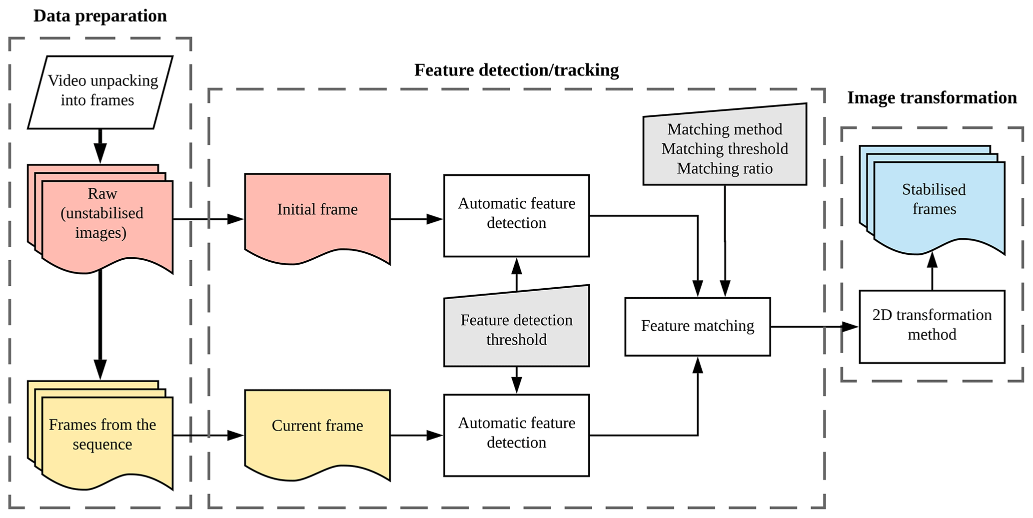
Some specific details of each examined tool are presented in the following sections, while more detailed descriptions are available in the repositories of the individual tools (Table A3). A general outline of the manual feature selection approach is summarised in Fig. 1.

Figure 1General outline of the manual feature selection/tracking approach. SA – search area; IA – interrogation area.
2.1.1 FFT-based tools: FFT-CUAS and FFT-DCH
FFT-based tools employ fast Fourier transform (FFT) cross-correlation in interrogation areas (IAs) around static features that experience apparent movement in order to estimate feature displacement from frame to frame.
FFT-CUAS (https://bitbucket.org/SIENA_Research/fishstream, last access: 21 February 2021) is based on the capabilities of freely available PIVlab MATLAB extension (Thielicke and Stamhuis, 2014), which is widely applied in the scientific community for particle image velocimetry (PIV) analysis (Le Coz et al., 2016; Dal Sasso et al., 2020; Detert et al., 2017; Detert and Weitbrecht, 2015; Lewis et al., 2018). The algorithm can be run in several iterations in order to increase the signal-to-noise ratio of cross-correlation. The size of the search area must be selected based on the expected frame-to-frame apparent motion of static features. Since the frame-to-reference displacement of static features may increase with the number of frames processed, the locations of the search areas are updated with each frame by centring them at locations of tracked static features. This accounts for the apparent motions of larger magnitude, when the frame-to-reference displacement of static features is more than half of the selected search area size. Image pre-processing/filtering available in PIVlab can be applied to the original images to increase the accuracy of FFT peak detection by enhancing image contrast and decreasing image noise. In order to increase the accuracy of displacement calculation, a 2×3 point Gaussian subpixel estimator is used. The type of image transformation (affine or projective) can be selected by the user.
Similar to the previous tool, FFT-DCH (https://github.com/salpeha/FFTVidStabilization, last access: 21 February 2021) is based on OpenPIV (Liberzon et al., 2020) and uses a cross-correlation technique based on FFT to estimate the frame-to-frame apparent motion. However, the implementation offers fewer options for feature tracking and transformation than FFT-CUAS. The frame-to-frame motion is determined by comparing four sub-windows of a frame to the corresponding windows of the previous frame. The user defines four points located at static positions in the image (e.g. no flowing water and no wind-moved vegetation), preferably at the corners, and the size of the sub-window (search area). The search area is then defined around these four points in the image. The size of the search area depends on the image resolution and the expected frame-to-frame apparent motion. At the time of the analysis, the available version of the tool did not allow the search areas to be updated with the positions of tracked features from the subsequent frames, which limits its applicability to those cases where subsequent frames do not deviate significantly from the initial frame of the video.
Even though both tools presented in this section are based on similar metrics, their implementation is significantly different, and their comparison will aim to expose the level of importance that the tool's implementation has in the overall accuracy and robustness of the stabilisation.
2.1.2 SSIMS: SSIM-based tracking
This tool (https://github.com/ljubicicrobert/SSIMS, last access: 21 February 2021) is based on an image comparison metric developed by Wang et al. (2004) and is implemented in the structural similarity (SSIM) stabilisation tool. A SSIM index can be used to compare two images of the same size and to assess their overall similarity. Unlike some image comparison metrics, such as the mean squared error (MSE), SSIM is significantly more robust in terms of global changes in brightness and contrast, as it implicitly relies on the information on shape, size, and orientation of features (structural information). A specific operator is convolved in the corresponding search areas from consecutive frames, which compare subregions from the current frame and the reference frame. This workflow generates a score map with values from −1 to 1, where 1 indicates a perfect match. The position of the maximal score indicates the likely position of the tracked feature in the current frame. To further improve the feature position detection accuracy, an arbitrarily sized Gaussian subpixel peak estimator is implemented. The positions of SAs are updated using positions of the tracked features. Both “fixed” and “updated” reference coordinate system strategies are implemented, but the use of the latter is generally only required for videos with a significant rotation of the ROI (usually >15∘) or significant scaling caused by altitude changes and/or camera zooming.
The tool also offers an option to estimate the per feature performance of the feature tracking stage by employing a specific root mean square difference (RMSD) analysis (post-tracking) to help the user to manually choose which of the tracked features are to be used in the image transformation stage. The image transformation can be performed using any of the possible homographic methods – similarity, affine, or projective – while also allowing least-square-based or RANSAC-based (random sample consensus; Fischler and Bolles, 1981) filtering of unacceptable feature correspondences.
2.1.3 KLT-IV: Kanade–Lucas–Tomasi tracking
This stabilisation approach is an inbuilt function within a MATLAB-based image velocimetry application tool KLT-IV (Perks, 2020) (https://sourceforge.net/projects/klt-iv, last access: 21 February 2021). This application has been developed for the generation of surface velocity estimates from cameras on both fixed and moving platforms (e.g. UAS). The reference coordinate system is defined by the first frame of the sequence, and subsequent images are aligned to it.
First, the strongest 10 % of detected corner points are automatically selected from each of the four quadrants of the image based on a minimum eigenvalue algorithm (Shi and Tomasi, 1994). This maximises the point distribution across the image and ensures that the strongest features are used in the stabilisation process. However, this approach is not fully automated as the user is required to define an ROI. The ROI polygon defines the areas within the image where motion occurs (i.e. where image velocimetry analysis should be focussed), and it is assumed that the area beyond this ROI is where the static features are located. Only the corner points retained in the first step that are located beyond the ROI are used in the stabilisation process. For each subsequent frame within the video sequence, corner features are detected and are matched to the points within the reference frame using the Kanade–Lucas–Tomasi (KLT) feature tracking algorithm composed of five pyramid levels. After the frame sequence has been stabilised, there is an option of running a second pass to stabilise the image sequence further. The difference between the first and second pass is that the search area (block size) is reduced in the second iteration. The first pass can, therefore, be seen as a coarse registration, with the second being a fine registration. The second pass is only required with videos exhibiting significant movement (e.g. Basento case study described in Sect. 2.4), with most deployments (e.g. Kolubara and Alpine case studies in Sect. 2.4) requiring a single pass for acceptable image stabilisation results.
2.1.4 Blender video editor
Blender (https://www.blender.org, last access: 21 February 2021) is a complete 3D modelling and animation suite which also contains a video editing suite with stabilisation capabilities. While not aimed specifically at either velocimetry or video stabilisation, Blender is a popular, free, and open-source off-the-shelf software which offers both manual and automatic selection of well-defined features. While it is clear from the user manual that the feature tracking relies on the IA/SA approach (similar to all previous tools), the metrics for the estimation of feature displacements are not clearly presented. However, we have included this tool in the comparison to investigate whether the use of dedicated tools is necessary for UAS video stabilisation purposes or if the general purpose software is accurate, fast, and simple enough to be used for this application.
2.2 Automatic feature selection approach
Advances in computer vision techniques have enabled automatic detection of well-defined image features which can be used to estimate the relationship between two images. Automatic feature selection algorithms aim to detect and describe specific, distinct features in an image, such as local corners or blobs, which display high pixel intensity gradients in at least two directions. For each feature detected, a descriptor is calculated that summarises the structure of the feature. For the purpose of image stabilisation, such detection and description can be performed for two consecutive frames from the video. Once such features have been automatically detected, feature matching is performed – their descriptors are compared, for instance, via calculating the Euclidean distance between n-dimensional descriptor vectors (Lowe, 2004). The main parameters of feature detection and matching methods are detection threshold (which determines the sensitivity of the feature detection and, therefore, the number of detected features), feature matching algorithm, matching threshold, and matching ratio. Once the feature pairs have been detected, a transformation matrix between the two images can be determined. Since automatic detection algorithms usually detect a relatively high number of feature pairs when compared to the approaches with manual selection of features, the possibility of outliers is increased and, therefore, their detection becomes necessary (e.g. RANSAC filter).
The general outline of automatic feature selection and tracking algorithms is presented in Fig. 2. Such algorithms generally do not require artificial GCPs in order to perform adequately, which can be a significant advantage for fieldwork in inaccessible terrain. However, the general absence of a priori knowledge on the stability and quality of detected features in the reference image requires the algorithm to collect a high number of candidate static features – often 100s or 1000s of features in order to obtain adequate results. Hence, the automatic feature selection strategy offers a benefit of lower operator involvement at a higher computational cost.
In this research, we investigated two stabilisation tools based on automatic feature detection algorithms, namely (1) features from accelerated segment test (FAST), presented by Rosten and Drummond (2006) and implemented by VISION (Pizarro et al. 2021), and (2) accelerated KAZE (AKAZE), proposed by Alcantarilla et al. (2013) and implemented by FlowVeloTool (Eltner et al., 2020).
Compared to other popular automatic feature detection algorithms, FAST is generally more computationally efficient. FAST detection and matching algorithms used in the tested stabilisation tool are implemented in a command line function written in MATLAB. FAST is able to identify edges as feature points in greyscale images with low scale changes, and a descriptor is then computed around the detected features using the fast retina keypoint (FREAK) algorithm. FREAK is a binary descriptor which accounts for changes in scale and rotation used to find feature points correspondences among images and is, therefore, stabilising. A RANSAC algorithm was also applied to remove false matches catalogued as outliers. In total, two variants of the approach were tested to (1) allow feature detection across the entire image or (2) select an ROI manually where the static features are most likely to be located. The latter approach can be thought of as a manual filtering stage, which can provide significant accuracy and efficiency improvement.
The last stabilisation tool tested is a part of a free and open-source velocimetry suite – FlowVeloTool (https://github.com/AnetteEltner/FlowVeloTool, last access: 21 February 2021) – which provides an option of using an accelerated KAZE (AKAZE) feature detection algorithm. AKAZE aims to detect scale-invariant features with low noise. The features themselves are detected as local extremes of the Hessian matrix at multiple scales. When the features are found, their descriptors are calculated. First, the dominant orientation is estimated to make the matching rotation invariant, and afterwards, a binary descriptor vector is calculated that performs pixel pairwise comparison. The matching ratio is chosen such that a match is determined as valid if the second-closest match reveals a significantly larger distance to the first match. In the stabilisation module of the FlowVeloTool, the AKAZE feature detector and descriptor and brute force matcher is used to find corresponding keypoints.
2.3 Image transformation
For the velocimetry purposes, all the analysed frames should exist in the same (reference) coordinate system so that real-world velocity estimation can be performed from in-image pixel displacements. When dealing with data that experience apparent motion, this is achieved by applying linear geometric transformation (homographic) techniques to raw images, i.e. similarity, affine, or projective transformation.
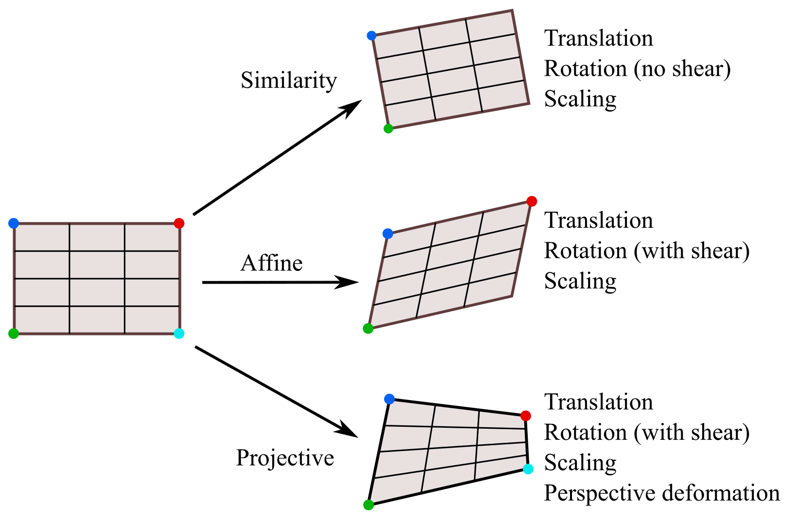
Linear image transformation is defined by three geometric operations, (1) translation, (2) rotation, and (3) scaling, and can be summarised by a matrix multiplication of the original pixel space as follows:
where x and y are the original point coordinates, x′ and y′ are the transformed point coordinates, and T is the transformation matrix. In the matrix T, a1…a4 represent the rotation and scaling parameters, and b1 and b2 are translation parameters. Image shear is defined within the parameters a1 and a4. Parameters c1 and c2 define the projection vector. In the case of the projective transformation, such parameters define the 3D rotation of the image plane around the horizontal and vertical image axes. All three approaches preserve collinearity and incidence. Similarity and affine methods also preserve parallelism, while the projective (in general) does not. In the affine transformation, c1 and c2 are zeros, while the similarity transformation is a special case of the affine method with shearless rotation. Due to this, both similarity and affine transformation methods are merely special cases of the projective method and are unable to account for image deformations in cases with significant pitch and roll rotations. However, as such cases are exceedingly rare in UAS velocimetry where the camera is optimally in nadir orientation, and all three transformation methods can potentially be used with comparable results. In cases where the pitch- and roll-type rotation of the camera can clearly be identified (e.g. aircraft operations in strong wind conditions), the use of a perspective transformation method is necessary in order to ensure proper stabilisation.
In order to define a transformation matrix T, relationships between two point pairs are needed for the similarity transformation, three pairs for the affine, and four pairs for the projective transformation. Examples of presented methods are presented in Fig. 3. Since all three described transformation methods are linear, as they transform an image from a plane in 3D space onto another plane, their accuracy will be impacted by the camera distortion parameters. If significant barrel- or pincushion-type distortion is present in the original image, these effects should be removed prior to the image transformation (MathWorks, 2021b; OpenCV, 2021).
2.4 Case studies
For the purpose of performance comparison of the presented tools, three case studies with different ground and flight conditions were analysed. The case studies were specifically chosen to exemplify a gradual increase in UAV motion intensity and complexity so that the limitations of specific tools can be adequately assessed.
-
UAS video with uniform GCP patterns and low camera movement (translation and rotation)
-
UAS video with various GCP patterns and moderate camera movement (translation and rotation)
-
UAS video without GCPs and with significant camera movement (translation, rotation, perspective deformation, and scaling).
The purpose of the first case study is to examine the performance of stabilisation algorithms in highly controlled conditions, such as low amounts of UAS/camera movement and vibrations, no significant rotation or altitude changes, and all GCPs being of the same pattern and positioned at the same level and at identical distances from the water surface. In total, six GCPs were positioned in the ROI – two 65×65 cm and four 20×20 cm in size (approx. 65×65 and 20×20 px in images, respectively), as shown in Fig. 4. However, not all control points were used in the stabilisation procedure; four points (marked GCP 1–4) were used for the stabilisation, and two (marked V1 and V2) were intentionally omitted in order to be used as verification points in the stabilisation accuracy analysis (method described in Sect. 2.5.2). This limitation was, understandably, imposed only onto those tools which employ manual feature selection. The experiment was conducted during low-flow conditions on the Kolubara river, in Serbia, in November 2018.

Figure 4Region of interest and the distribution of ground control points for the case study 1 – Kolubara river.
The video from the second case study contains a moderate amount of UAS/camera movement, and all GCPs are of the same size (66×33 cm; approx. 32×16 px in images) but have different patterns and were not positioned on the same elevation. The experiment was conducted in June 2019 on an Alpine river in Austria, with an ROI of approx. 80×45 m. The flight was conducted in favourable weather conditions. In total, eight GCPs were positioned in the ROI (marked as GCPs 1–8 in Fig. 5). The presence of islands in the middle of the ROI provided an opportunity for an analysis of the residual motion in the centre of the ROI (method described in Sect. 2.5.1) where velocimetry analyses are usually performed. To estimate the overall motion in the centre of the ROI, motion analysis was performed on the regions indicated in Fig. 5. The three additional points (marked V1–3), representing static features in the centre of the ROI, are used for displacement estimation (method described in Sect. 2.5.2).
Both previous case studies involve the use of GCPs for image stabilisation in relatively controlled conditions. The third case study conducted on the Basento river in Italy (ROI presented in Fig. 6) aims to investigate whether the analysed stabilisation tools are applicable to a video with no artificial GCPs or well-defined static features, which also contains a high amount of camera movement (Dal Sasso et al., 2020; Pizarro et al., 2020). A black-and-white pole was placed in the ROI during the video recording and was later used to identify the ground sampling distance of 0.5 cm px−1. The unfavourable video recording conditions were expected to be more challenging for the stabilisation tools and could help with the identification of the limitations of specific approaches.
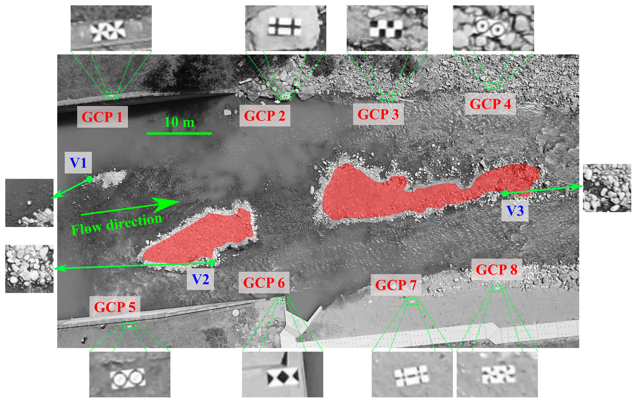
Figure 5Region of interest and the distribution of ground control points for case study 2 (Alpine river). Red coloured regions are later used for displacement analysis, using surface velocity fields (SVFs), in Sect. 2.5.1.
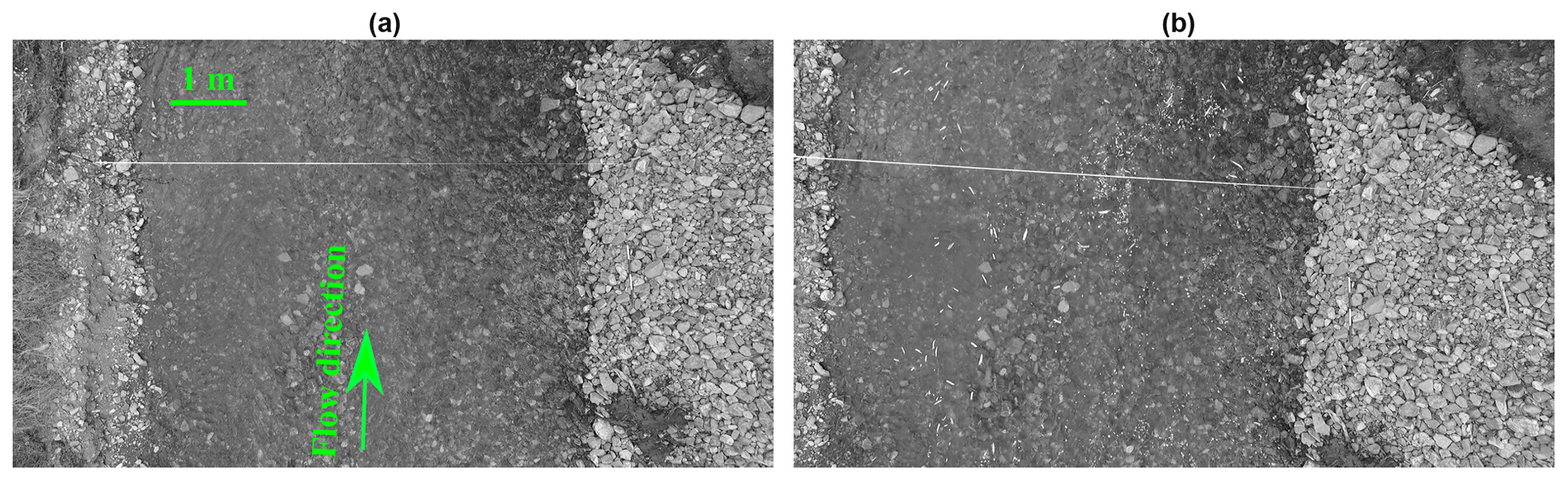
Figure 6Region of interest in case study 3 (Basento river). (a) Initial frame. (b) Frame no. 700.
Greyscale images were extracted directly from the UAS videos and were not preprocessed or filtered in any way prior to the stabilisation. Frames from the Kolubara and Basento studies were extracted at original frame rates, but for the Alpine case study every fifth frame from the original video was extracted and used in order to further increase the amount of apparent inter-frame motion. Relevant metadata of the videos used in this study is presented in Table 1, while the location of the data set with both unstabilised and stabilised images is listed in Table A3.
Table 1Metadata of the videos used in this study.
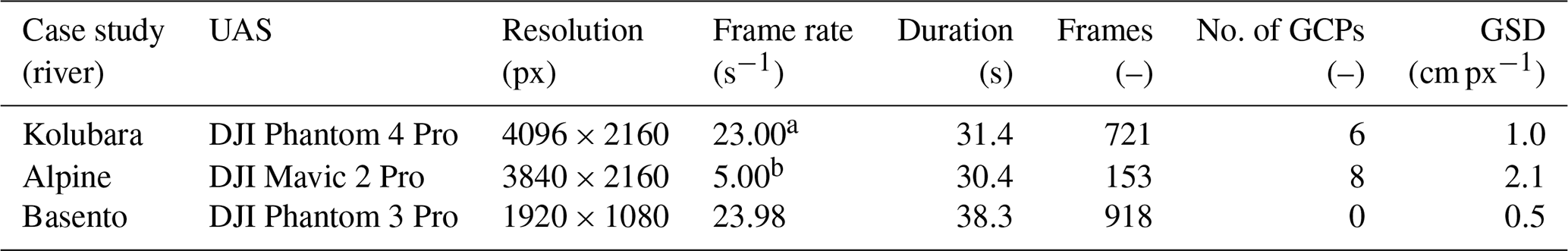
GSD – ground sampling distance. a Resampled from 23.98 frames per second due to code library limitations. b Resampled from 25 frames per second.
2.5 Comparison metrics
In order to evaluate the performance of stabilisation algorithms, it is necessary to measure the residual displacement of static features in the stabilised frame sequences, i.e. stabilisation errors. Considering that the residual displacements are both spatially and temporally distributed in the stabilised frame sequences, both distributions should be adequately described. For this reason, we have used a combination of two approaches for performance assessment:
-
For the estimation of the spatial distribution of residual motion, we have applied a surface velocity field (SVF) analysis between the initial frame and a selected number of frames from the sequence. Such analysis was only performed on those regions of the ROI, which are comprised of static features. This strategy has the benefit of illustrating the type of apparent motion (e.g. translation, rotation, tilt, and scale change) observed in a frame sequence. However, such analysis can only be effectively used for the analysis of a relatively small number of frame pairs since the character and intensity of the spatial distribution of residual motion cannot be efficiently summarised for the entire frame sequence unless motion type and intensity do not vary.
-
For the estimation of the temporal distribution of residual motion, we describe and propose an alternative metric for the estimation of the magnitude of the residual displacement of static features based on a pixel intensity root mean square differences (RMSDs). This metric can be effectively applied across the entire frame sequence for a small number of selected static features. In the case of this research, such static features were verification points denoted with a V number in Figs. 4 and 5. An additional benefit of this metric is that it is not contained within any of the feature displacement estimation techniques used by the analysed stabilisation tools; hence, no bias towards individual methods is expected. However, this method does not provide information on the actual type of motion.
Considering the aforementioned characteristics, the two comparison metrics aim to provide complementary insights into the types, intensities, and (potentially) sources of errors for different stabilisation tools.
2.5.1 SVF analysis
Surface velocity field estimation is performed for some of the representative frame pairs in order to estimate the performance of stabilisation algorithms when dealing with different types of camera motion. When applied to stabilised frames, SVF analysis allows assessment not only of the magnitude of residual displacement, but also of its direction, thus exposing the strengths and weaknesses of the stabilisation approach. The disadvantage of this approach is its computational complexity and difficulty of generalising results.
For the Kolubara case study, we analyse four frame pairs formed by combining the initial frame (no. 1 in the sequence) with each of the frame nos. 51, 151, 351, and 551. These frames were selected as (1) they illustrate different types of motion (i.e. tilt, rotation, scale change, and the combination of the latter two), and (2) the motion magnitude is sufficient for unambiguous visual identification of the motion type. For each of the frame pairs, dense surface velocity fields are calculated with the use of FFT cross-correlation implemented in PIVlab and then aggregated to eight vectors which characterise eight subregions of the ROI (Fig. 7). The choice of subregions was motivated by the following criteria: (1) they contained no moving features, (2) they were sufficiently lit, and (3) after summarising the vectors to one per subregion, the level of detail was still sufficient for determining the type of the residual apparent motion.

For the Alpine case study, SVFs are calculated for both islands (see Fig. 5) located in the middle of the river and averaged to one vector per island. Since camera motion in this case study has the same direction throughout the image sequence, SVF analysis is performed for one frame pair for each stabilised image sequence. This frame pair (nos. 1 and 152) is selected with the goal of maximising the magnitude of an apparent frame-to-reference motion of static features, which gradually increases towards the end of the frame sequence.
2.5.2 Point displacement through RMSD
In order to allow for an automated quantification of residual motion magnitude in the entire image set, we propose a 2D root mean square difference (RMSD) metric which operates by directly comparing a number of subregions within subsequent images. The aim of the proposed method is to provide a quantitative description of subpixel displacements that is easier to compute directly from images. Small rectangular subregions were sampled from stabilised images, and these regions were compared to the same regions from the reference frame. The differences in pixel-wise intensities between the subregion pairs are likely to indicate the similarity of the two regions and, subsequently, the quality of the image stabilisation. For two subregions from images A and B, with heights and widths N×N (where N is an odd number) and centres at (x0, y0), we define , so that the RMSD can be calculated as follows:
where YA and YB are the single channel (e.g. greyscale) pixel intensities from images A and B, respectively. This comparison can be performed for a number of chosen feature points in the images. The average RMSD from all features in the frame sequence represents the total score of the selected method, with a lower score indicating a higher similarity between the compared subregions and, therefore, a higher stabilisation accuracy. The choice of comparison features, and the size of the examination subregion, were presented for each relevant case study in Sect. 2.4.
Similar to the feature tracking strategies, the following two approaches can be applied: (1) using the initial frame as the reference frame and (2) frame-by-frame comparison. The former criterion is important when an accumulation of errors is possible in the stabilisation algorithm and mostly describes the impacts on the pixel positioning accuracy, while the latter can be a better estimate on the overall impact on velocimetry results, as velocimetry also uses a frame-by-frame comparison method.
The use of the first frame as the reference for matching subsequent frames, as opposed to an approach where the reference is the previously stabilised frame in the sequence, is beneficial because the potential for drift in the stabilised output is eliminated. However, a limiting factor is that the reference frame must share a significant portion of the field of view with each image within the sequence to enable features to be matched.
The goal of the analysis is to establish a correlation between the easily calculable RMSD and the actual displacement d in the form of d=f(RMSD), so that the temporal distribution of residual displacements can be efficiently estimated. Parameters used by each of the tools to produce the stabilised images are presented in Table A1 in the Appendix.
In this section, we present the analyses of the stabilised image sets. In order to obtain the best performance from each of the stabilisation tools, the authors of the respective tools were provided with the unstabilised videos and given the task to provide the best stabilisation performance possible, using their own tools. No restrictions regarding the number and choice of static features were imposed, other than the exclusion of verification points (see Figs. 4 and 5) which would later be used for the stabilisation accuracy analysis. Finally, no restrictions were imposed regarding the choice of the image transformation method – authors were given the freedom to choose the approach they found suitable for each case.
3.1 SVF analysis
The SVF analysis of the unstabilised video for the Kolubara case study revealed that the magnitude of apparent motion in four selected frame pairs was between 4 and ∼38 px. Frame pairs illustrating rotation and rotation/scale change were characterised by the greatest instability. Vector fields illustrating details for the eight subregions of the ROI in each of the unstabilised frame pairs are displayed in Table 2.
Table 2Aggregated results of the SVF analysis of the unstabilised video for the Kolubara case study. The mean u and v components of the apparent motion of static features in eight subregions are illustrated by vector size and orientation, whereas numeric values illustrate the mean apparent velocity magnitude for each subregion.
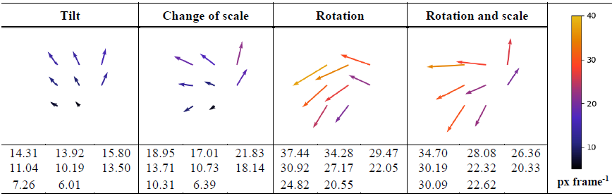
Table 3 presents residual SVFs calculated for each of the four representative frames in the data sets stabilised with different tools, averaged for each of eight subregions of the ROI. The residual apparent movement of static features has a magnitude of less than 3 px for all the analysed stabilisation tools, whereas for many of them it is below 1 px on average. According to SVF analysis, the most stable subregion in the frames processed with FFT-CUAS is located on the left side in the middle of the ROI along the river (subregions 2, 4, and 6 in Fig. 7). The subregions 7 and 8 on the right riverbank are characterised by a mean apparent residual motion of ∼0.5 px in the direction opposite to the direction of the original displacement. The mean magnitude of residual displacement of the static features in the ROI after stabilisation with FFT-CUAS is ∼0.33 px. FFT-DCH, which employs a feature tracking algorithm similar to FFT-CUAS, performs differently, with a residual feature displacement of ∼1.09 px on average, and exposes a residual anticlockwise circular motion for each of the four different types of original motion. Frames stabilised with KLT-IV preserve some residual circular motion in cases when original frames experience rotation. In the case of scale change, KLT-IV and FAST slightly overcompensate the motion in the original frames. The mean residual displacement of static features was 0.66 px for KLT-IV and 0.74 px for FAST. In the case of tilt, the FAST stabilisation approach leads to multidirectional residual feature displacements on the left-hand side of the field of view (subregions 1, 3, and 5). These displacements compensate for each other during averaging, resulting in a discrepancy between the mean vectors and the mean velocity magnitudes in the area. This example illustrates the complexity of the generalisation of SVF analysis results in the case of multidirectional residual displacement of static features.
Residual displacement of static features in frames stabilised with SSIMS was 0.60 px on average. The directions of vectors indicate that the scale of images after stabilisation is slightly different from the original scale; this difference, however, lies in a subpixel range. The highest residual displacement in frames stabilised with SSIMS (0.78 px on average) is observed in the case when the original frame experiences rotation (similar to KLT-IV). Frames stabilised with AKAZE indicate average residual feature displacement of 0.76 px and experience a similar pattern with the right bank being more stable than the left bank, especially when compared to the leftmost part of the images in subregions 1 and 3. Blender/M results are characterised by the residual feature displacement of 0.68 px on average. Similar to KLT-IV and FAST, Blender/M slightly overcompensates the motion in the case of scale change. It also preserves some anticlockwise motion in cases of rotation. A peculiarity of image stabilisation with the use of Blender/M is the change in image colour. Visual analysis of this change indicates contrast reduction, which complicates the identification of traceable features (Fig. 8).
Overall, SVF analysis results of the first case study indicate that most of the analysed stabilisation tools transform raw frames in a way that the residual displacement of the static features lies in a subpixel range. For the second case study, residual displacement of the static features was estimated for the two islands in the middle of the river, since the stability of this region is of the most interest because it is the focus of the image velocimetry analysis. SVFs calculated for both islands were further averaged to one vector per island (Table 4).
Table 3Aggregated SVF analysis results of the stabilised videos for the Kolubara case study. The mean u and v components of the residual motion of static features in eight subregions are illustrated by vector size and orientation, whereas numeric values illustrate the mean residual velocity magnitude for each subregion.
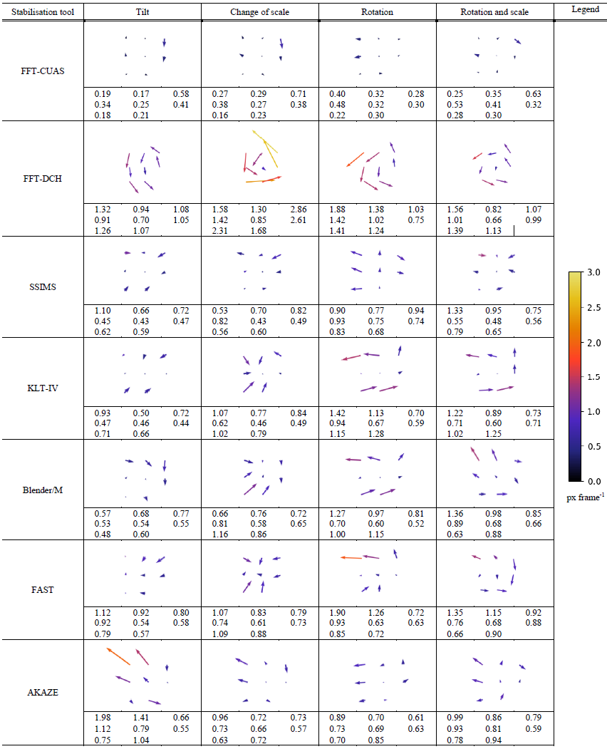
Table 4Aggregated SVF analysis results of both unstabilised and stabilised videos for the Alpine case study. The mean u and v components of the apparent motion of static features on each of the two islands are illustrated by vector size and orientation. Numeric values illustrate the mean apparent velocity magnitude for both islands.
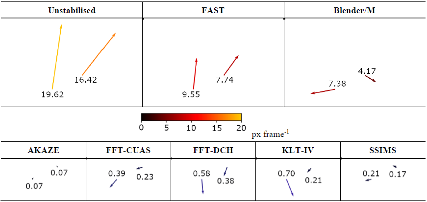
Analysis of the residual SVFs for the Alpine case study indicated that FAST has not managed to compensate for the apparent motion in the original frame sequence but rather decreased its magnitude. Similar to the Kolubara case study, Blender/M significantly overcompensated for the apparent motion in the raw frames and has changed the colours in the images, reducing the contrast and complicating the recognition of traceable features (Fig. 8). The residual displacement of static features in the frames stabilised with AKAZE, FFT-CUAS, FFT-DCH, KLT-IV, and SSIMS was in the subpixel range, mostly below 0.5 px. Static features on the left island experienced more residual displacement regardless of the stabilisation tool used, with the exception of AKAZE. Residual displacement of the static features on the islands after stabilisation with AKAZE is the least among all stabilisation tools. It is, however, important to keep in mind that, due to the automatic feature selection mechanism, AKAZE used static features on the islands for image stabilisation, which was likely to increase their stability.

Figure 8Alpine case study. (a) Original image section. (b) Image section after stabilisation with Blender/M, with noticeable changes in contrast.
SVF analysis of two case studies has shown that stabilisation with AKAZE, FFT-CUAS, SSIMS, and KLT-IV predominantly results in a residual displacement of static features in subpixel range. FFT-DCH, Blender/M, and FAST have a less consistent performance, resulting in higher magnitude of residual displacement in one of the case studies than in the other. Blender/M was the only tool whose application resulted in colour changes that may have a negative influence on the quality of subsequent image velocimetry analysis.
3.2 Point displacement through RMSD
To examine the adequacy of the proposed RMSD metric for use instead of manual planar displacement measurements, we devised a synthetic test. Using the initial frames from the original videos, displacements were induced by artificially shifting the images in the horizontal and vertical direction by Δx and Δy pixels (both positive and negative displacements were considered). To find suitable validation points, a number of candidate points were manually selected, and the d(RMSD) relationship was determined. Candidate points with high R2 of the d(RMSD) were selected as validation points, and these are marked with V numbers in Figs. 4 and 5. The results of the analysis are presented in Figs. 9 and 10 and demonstrate the following:
-
The RMSD score generally depends on the size of the interrogation window, defined by its width/height N. The size of the interrogation area around the selected feature points was gradually increased while calculating the corresponding R2. Optimal IA size (N=31 px) was selected to be the one with the maximal average R2 for all features.
-
For displacements of up to 4–5 px, the relationship between d and the RMSD score fits a second-degree polynomial for all validation points. The coefficients of the fit (a, b) were determined for the polynomial relationship as follows:
By using Eq. (3), one can estimate the displacements d from RMSD scores. The accuracy of the estimation is highest for low displacements but deteriorates quickly for displacements higher than 4–5 px. Coefficients a and b are presented in Table A2 in the Appendix for individual validation points.
-
For displacements lower than 7–8 px, the relationship between d and the RMSD score is monotonic. It was determined that this relationship is correlated to the size of the static feature used for validation.
-
For displacements larger than 7–8 px, the RMSD plateaus or even decreases. This can be explained by the loss of the tracked static feature from the search area for large displacements. Once the search area contains only the unstructured background pattern, the RMSD approach is unable to quantify further displacements due to increased likelihood of ambiguities, and the relationship between the RMSD and d is undefined.

Figure 9Displacement as a function of RMSD of pixel intensities. (a) Kolubara case study. (b) Alpine case study.

Figure 10Second-degree polynomial fit of the d(RMSD) relationship for low displacements. (a) Kolubara case study. (b) Alpine case study.
Synthetic tests indicate that the RMSD can be an adequate representation of planar displacement d in cases where the displacement between two images is within the area where the second-degree polynomial provided a high R2 (<4–5 px). This condition was satisfied for any two consecutive frames of both the unstabilised and stabilised frame sequences of case studies 1 and 2. If the initial frame is used as a reference, the condition was satisfied only for the stabilised frames. For the raw frame sequence, the displacements d obtained through RMSD scores are likely to be underestimated due to increased chances for ambiguities for large displacements in which case the proposed approach is unsuitable. The intercept term in the polynomial relationship in Eq. (3) was intentionally omitted in order to retain some “physical” meaning in the relationship and prevent the equation from indicating small displacements even when RMSD = 0. Using the d(RMSD) metric defined by Eqs. (2) and (3), displacements of validation points were estimated in every frame of the stabilised sequences. Estimated displacements are summarised in the form of standard box plots in Figs. 11 and 12 for the Kolubara river case study and Figs. 13 and 14 for the Alpine river case study. Blender software was excluded from the pixel-intensity-based comparison due to the previously described colour grading issues, which caused a positive bias towards this stabilisation tool.
Figures 11 and 13 summarise all displacements of validation points across the entire frame sequence relative to their location in the initial frame and aim to present the susceptibility of tools towards error accumulation over the course of long frame sequences. Such accumulation could potentially lead to vector positioning errors, as points in the ROI would gradually drift away from their initial positions. Based on the results obtained, several tools have demonstrated adequate results with predominantly subpixel errors in both case studies, i.e. FFT-CUAS, SSIMS, KLT, and AKAZE. The latter had provided the best results in both studies considering both median values and the overall variability, with all estimated displacements in the subpixel range. Even though it employed the simplest image transformation method (similarity), KLT-IV also demonstrated only subpixel displacements in the Kolubara study, with generally low variability and median values below 0.5 px; in the Alpine study, the errors are somewhat higher but still comparable with the best-performing tools. SSIMS and FFT-CUAS results were very similar, with medians below 0.5 px, and low variability, with FFT-CUAS showing marginally lower errors in the Kolubara case and SSIMS in the Alpine case. While the results seem to confirm the expected bias of PIVlab towards the FFT-CUAS in the SVF analysis, the d(RMSD) metric confirms that FFT-CUAS objectively presents adequate results comparable with all other well-performing tools. The two remaining tools – FFT-DCH and FAST – had shown significantly higher residual displacements. Displacements after stabilisation with FFT-DCH and FAST were up to 4.3 and 2.8 px in the Kolubara case, respectively. In the Alpine case, the results obtained using FAST are above the applicability limit of the Eq. (3), with indicated errors of up to 7 px. Further inspections of the stabilised video obtained using FAST had shown that the raw motion of the camera/UAS was not properly counteracted but rather decreased in intensity. In the Alpine case study, FFT-DCH had provided results comparable with KLT-IV, SSIMS, and FFT-CUAS, with predominantly subpixel errors and median values between 0.4 and 0.8 px. This is potentially indicative of high sensitivity of the FFT-DCH tool to different ground conditions and/or parameter changes.
The results of frame-to-reference d(RMSD) analysis generally substantiated the results of the SVF analysis. Interestingly, even though they employ different algorithms, almost all the tools demonstrated higher median errors and variability in the same regions – e.g. the right riverbank in the Kolubara case and leftmost island in the Alpine case – according to both evaluation metrics. The exact cause of higher displacements of static features in these regions (compared to the features in other sections of the images) was not definitively identified in this study and could be related to both flight and/or ground conditions. Figures 12 and 14 summarise all displacements of the validation points across the frame sequence relative to their position in the previous frame. Due to the frame-by-frame nature of this analysis, it is more likely to be directly correlated to the image velocimetry results. When compared to Figs. 11 and 13, results obtained using different tools show fewer differences, with all tools now demonstrating median errors below 0.5 px in the Kolubara case and 0.65 px in the Alpine case. However, the total number of outlier values is higher than when compared to the initial frame (Figs. 11 and 13), which can in part be explained by the potential overcompensation of motion between two consecutive frames which leads to artificially induced oscillations (jitter) in the stabilised images. AKAZE still demonstrates the lowest displacements, followed by (in order of decreasing accuracy and the average of the two case studies) KLT-IV, SSIMS, and FFT-CUAS. The apparent displacements in the results of FFT-DCH and FAST are considerably lower when displacements are estimated relative to the previous frame, i.e. when the effects of error accumulation are not considered.
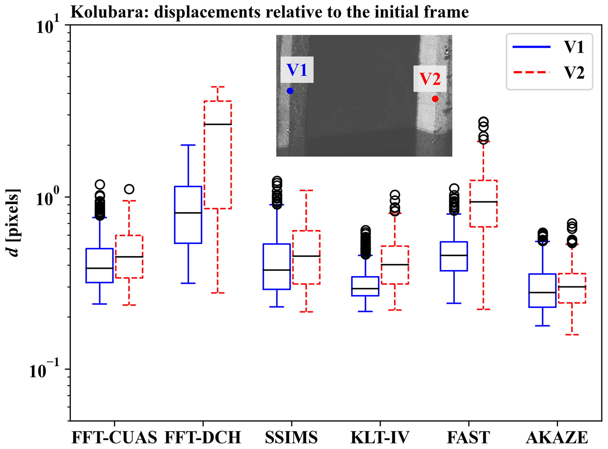
Figure 11Displacements of validation points relative to their positions in the initial frame for the Kolubara river case study.
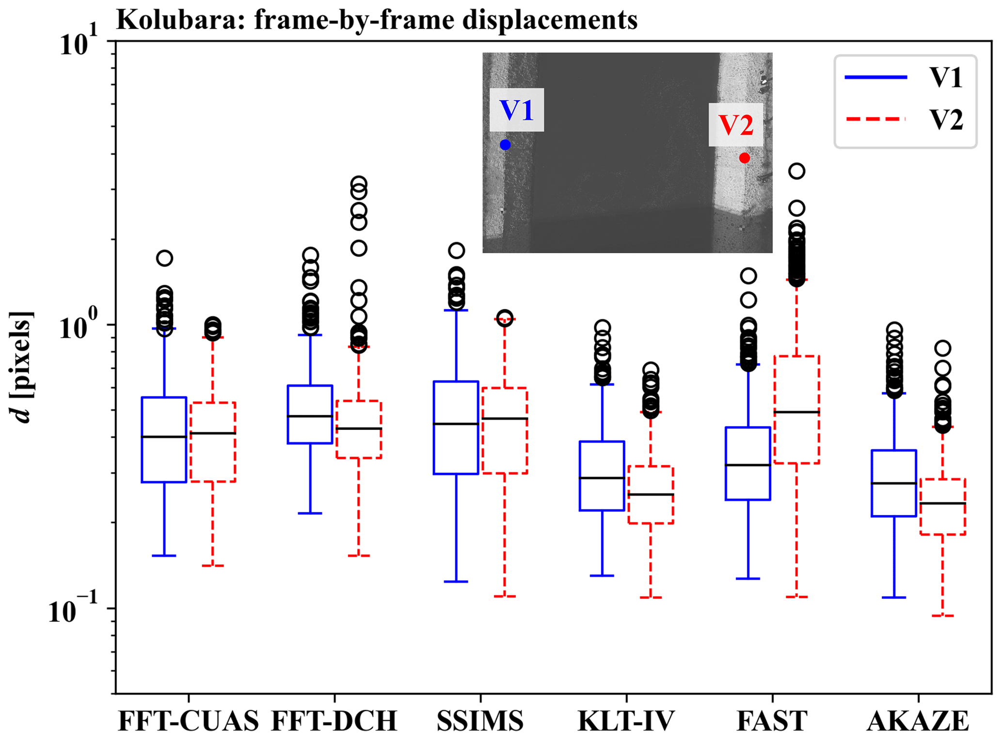
Figure 12Displacements of validation points relative to their positions in the previous frame for the Kolubara river case study.
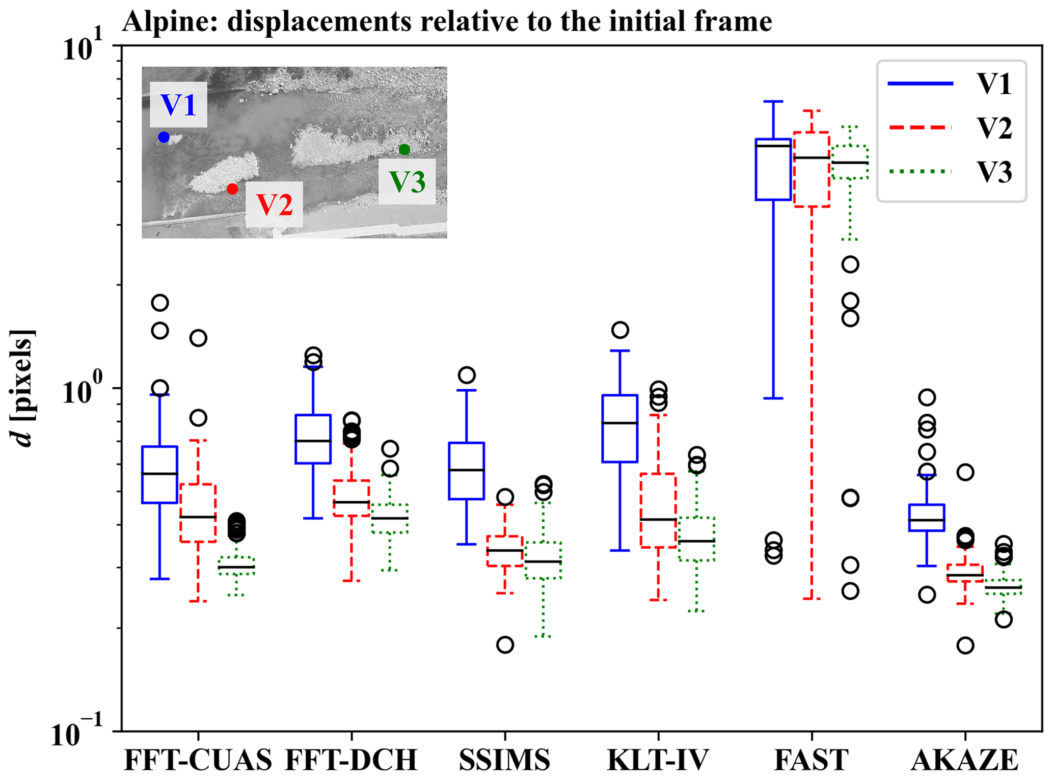
Figure 13Displacements of validation points relative to their positions in the initial frame for the Alpine river case study.
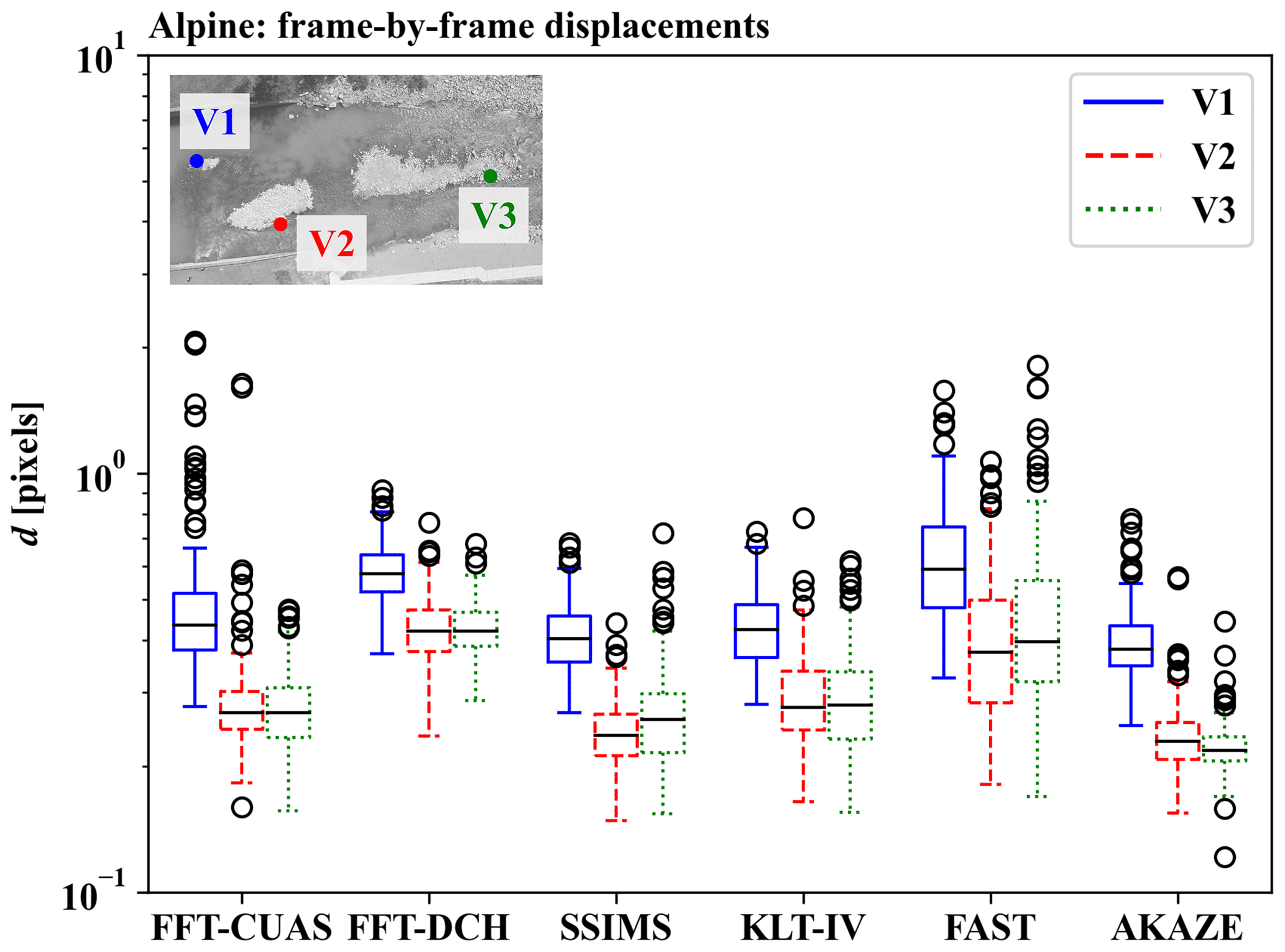
Figure 14Displacements of validation points relative to their positions in the previous frame for the Alpine river case study.
Analysis of the Basento river case study proved to be more challenging than the previous two, considering the complete lack of GCPs or unique static features, as well as the variety and intensity of the camera/UAS motion with sudden strong translation and rotation exacerbated by changes in scale. For these reasons, the comparison was only performed qualitatively based on the criteria of jitter intensity (sudden and strong movement induced by stabilisation tool inaccuracy rather than actual camera motion), residual motion intensity (original camera motion that was not accounted for by the stabilisation tool), and the presence of undesirable deformation of the water surface area (ROI) caused mainly by the parallax effect (defined by the apparent differences between image foreground and background motion). The results are presented in Table 5.
Out of seven tools tested, only FFT-DCH was not able to complete the stabilisation on the entire 38 s of video. In total, three tools were able to stabilise the video adequately and completely, namely FFT-CUAS, SSIMS, and Blender/M. However, the colour grading issue in Blender significantly deteriorates the quality of surface tracers which are meant to be used in image velocimetry. The results obtained using KLT-IV were significantly impacted by the sudden reduction in the visible part of the left riverbank, which had caused moderate but persistent jitter throughout the remainder of the sequence. AKAZE and FAST, which employ a fully automatic selection of static features, have demonstrated severe jitter and/or residual motion in the results, which were likely also caused by the sudden loss of riverbank features on the left-hand side of the video frames. As with the Alpine case, FAST was also not able to properly counteract the original motion but instead reduced its intensity. While seemingly compensating for the general camera motion, AKAZE produced significant jitter on the left riverbank that persisted throughout the entire video. To test the hypothesis that automatic feature selection leads to lower stabilisation quality in challenging video recording conditions, we performed another stabilisation using Blender in an automatic feature selection mode (Blender/A). When allowed to automatically select the static features, Blender/A periodically produced jittery motion because the occasional escaping of the tracked features from the frame, combined with the parallax effect, had caused ROI to experience deformations.
Table 5Qualitative comparison of stabilisation results for case study 3 – Basento river.

∗ Could not be estimated due to jitter
To examine the complexity of the stabilisation procedure using different tools, we have timed the procedures of feature tracking and image transformation. The average per frame stabilisation time is presented in Table 6, along with the RAM usage range throughout the stabilisation process. The latter information was included to demonstrate the generally high requirements of the off-the-shelf software when compared to purpose-specific tools. Table 6 also includes information on the stabilisation capabilities of the tools with regards to rotation and scale changes, capabilities for simultaneous orthorectification of images when real-world positions of static features are known, and the availability of an accompanying graphical user interface (GUI). Finally, we present the information regarding the programming language requirements for each tool and a short summary of other capabilities of the specific tools.
Table 6Summary of capabilities, complexity, and limitations of different stabilisation tools, based on the Kolubara case study.
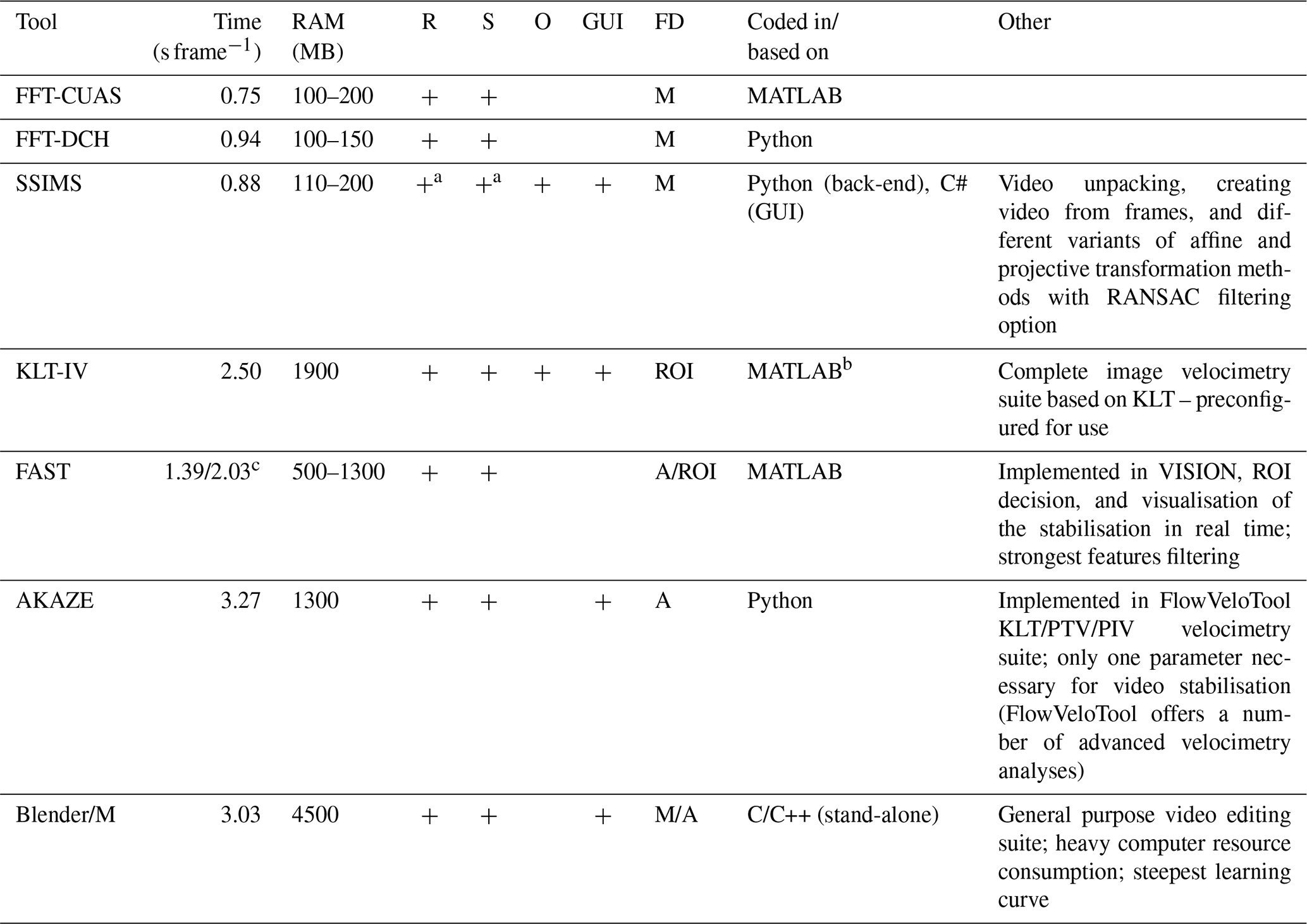
a With kernel updating, at the cost of somewhat lower feature tracking accuracy. b Compiled and can be used without MATLAB installation. c ROI selected/without the ROI selection. R – rotation; S – scaling; O – orthorectification; GUI – graphical user interface; FD – feature detection approach (M – manual; A – automatic; ROI– ROI selection).
The results presented in the previous section aim to illustrate the importance of image stabilisation in velocimetry analyses. Even in favourable weather conditions, motion induced by the UAS platform is far from insignificant. Flow conditions in the Kolubara case study indicated low average surface velocity of approx. 0.12 m s−1, while the orthorectified images had a ground sampling distance (GSD) of 1 cm px−1 (Pearce et al., 2020). The Alpine river case had a somewhat higher GSD of 2.1 cm px−1, and reference velocities (obtained using a current meter) were between 0 and ∼2 m s−1 (Strelnikova et al., 2020). The Basento river video was captured at the lowest flight altitude and, despite also being captured in the lower resolution, had the GSD of 0.5 cm px−1, with the average surface velocity of 0.40 m s−1 (Dal Sasso et al., 2020; Pizarro et al., 2020). Considering the results presented in the previous section, stabilisation error of even a few pixels per frame could potentially induce significant errors in estimated instantaneous velocities. Another important aspect of stabilisation is preventing the aggregation of camera motion (positional drift) over the course of the video. For that reason, motion in the stabilised data sets has been estimated both relative to the initial frame (SVF and d(RMSD) metrics) and relative to the previous frame in the sequence (d(RMSD) metric only) in order to identify which tools are susceptible to such error aggregation and to what extent.
Using SVFs as a metric of image stabilisation quality has the advantage of providing information about the spatial distribution and type of residual motion. This approach, however, has high complexity and is unsuitable for processing a large number of frames. Frame-to-frame feature displacements in the opposite directions may compensate each other during averaging, creating a false impression of stability. A median-based generalisation is more robust than averaging, but there can still be disparities between the median velocity magnitudes and the velocity vectors calculated as median values of u and v vector components. Aggregation of SVFs can lead to meaningful conclusions with regards to the type and the magnitude of apparent motion in a frame sequence only if motion type and direction do not vary greatly across the frames. Frame sequences can be divided into parts characterised by the same type of apparent motion, and SVFs may be aggregated for each of the subsequences. However, this only increases the complexity of using SVFs as an evaluation metric.
Considering the proposed d(RMSD) metric, we demonstrated that it can be effectively used for estimation of displacements of up to 4–5 px. It is important to note that the conclusions regarding this metric presented in Sect. 2.5.2 are derived for the case studies described in this paper and should not be generalised. However, the methodology can be applied to any image set if suitable validation points can be obtained, as would be indicated by high R2 value. Unlike the SVF analysis, d(RMSD) does not provide any detail on the character of the residual motion, i.e. translation, rotation, scale, or a combination. Finally, the proposed metric assumes that no significant changes in brightness are present during the video, as such changes would affect the RMSD score even if no actual displacements are present. Since the videos from the selected case studies were relatively short (up to 38 s), no global or local changes in brightness were observed.
Considering that FFT-CUAS uses the cross-correlation code of PIVlab to produce stabilised videos, it was possible that PIVlab-based SVF analysis results could be biased towards this stabilisation tool. Therefore, the stabilisation accuracies of all tools were verified using the relationship between pixel intensity RMSD and pixel displacement d for several validation points in the Kolubara and Alpine river videos. While the results seem to confirm the presence of such SVF analysis bias towards FFT-CUAS, its reported accuracy according to d(RMSD) is still objectively high and comparable with other best-performing stabilisation tools. The bias of the SVF approach using PIVlab towards other tools was not evident in this research, and the SVF results are generally comparable with d(RMSD) metric. The performance of any given stabilisation tool seems to depend on its implementation in the given tools and the feature detection/tracking algorithm. This is most obvious when comparing the results between the two approaches based on cross-correlation techniques – FFT-CUAS and FFT-DCH. While both are based on 2D cross-correlation algorithms, the implementation of the FFT-CUAS is more flexible towards different ground and flight conditions. A similar argument can be made for FAST and AKAZE; while both rely on automatic feature detection algorithms, the implementation of the state-of-the-art AKAZE feature detection algorithm in the FlowVeloTool is supported by an optimised feature matching approach which enables more consistent and accurate stabilisation. This conclusion is further reinforced by the fact that several feature tracking metrics have been able to deliver similar assessments of stabilisation accuracy, regardless of different underlying methodologies.
Considering the first two case studies, which aim to depict common UAS velocimetry conditions, four tools have been able to provide adequate results (i.e. FFT-CUAS, SSIMS, KLT-IV, and AKAZE). The automatic tool AKAZE, implemented by the FlowVeloTool, demonstrated the highest median stabilisation accuracy of all the investigated tools. The abundance of static features in the Kolubara and Alpine cases can potentially favour automatic feature detection algorithms if such features are evenly spread out in the ROI. No constraints were imposed on the FAST and AKAZE with regards to the areas in which the features could be detected, which allowed those tools to potentially use validation points for the estimation of the optimal transformation matrix and the central islands from the Alpine case. While this degree of freedom could potentially create a bias towards such tools in the d(RMSD) analysis, it was assumed that such bias is relatively low due to the sheer number of features detected by both FAST and AKAZE, and this was not considered in this research.
In the group of manual feature selection tools, FFT-CUAS, SSIMS, and KLT-IV provided accurate stabilisation with subpixel median accuracy, but no tool was dominantly more accurate than the others when both cases are considered. KLT-IV had proven to be capable of consistent sub-0.5 px accuracy in cases with low inter-frame motion and low camera tilt, such as in the Kolubara case. FFT-CUAS and SSIMS results were the most similar among the examined tools, which is not surprising considering the fact that the implemented SSIM-based stabilisation is (at least in part) inspired by the principles of the PIV/PTV (particle tracking velocimetry) techniques, while the FFT-CUAS tool uses segments of the PIVlab code base. On the other hand, several tools have demonstrated inconsistent performance between the Kolubara and Alpine river case studies; FFT-DCH displayed significantly better results in the Alpine river case study than in the Kolubara case study, while FAST and Blender/M demonstrated the opposite change. This indicates an increased sensitivity of those tools towards different ground and flight conditions, GCP size and/or GCP patterns, among others.
Some performance differences could be explained by the fact that the GCPs in the Alpine river video were not positioned on the same elevation; those in the upstream (left) parts were positioned around 4 m higher than the rest. Considering that the homographic image transformation assumes plane-to-plane relationship between point pairs, differences in GCP elevations have likely induced additional errors which are evident for the results of all investigated tools. For example, Figs. 12 and 14 demonstrate that verification point V1, located between the two elevated GCPs, is characterised by lower stability than the other control points. The same is confirmed by the SVF analysis, where static features on the left island experienced more residual displacement regardless of the stabilisation tool used, with the exception of AKAZE. To alleviate such issues, it is recommended that stabilisation, whenever possible, is performed with the use of static features with the same elevation. In cases where this principle cannot be followed, estimating the transformation matrix by using a higher number of features than minimal (for the chosen transformation method) can limit the extent of such errors. This can potentially explain the high accuracy of AKAZE in the Alpine case where it used approx. 400 features to estimate the transformation matrix.
The distribution of GCPs and/or static features should also be considered. As a rule of thumb, the GCPs should be positioned as close to the water surface as practically possible in order to limit the parallax effect; if the water surface and the plane holding the GCP are on different elevations, motion of the camera can introduce a parallax effect demonstrated by the apparent motion of the two planes relative to each other. The intensity of this effect depends mostly on the ratio of distances between the UAS and the water surface and the UAS and the GCPs and, thus, can also be limited by operating the UAS at higher flight altitudes. Additionally, such effects depend on the focal length of the camera – short focal lengths are more susceptible to the parallax effect. With tools relying on manual feature selection, it is beneficial to choose only the features closest to the water surface as this would substantially reduce the parallax effect. If the features are automatically selected from the entire image, there is no guarantee that they will be selected from the same elevation, unless some constraints are imposed with regards to areas in which the features are detected.
In the Basento river video, which aims to demonstrate a case with complex camera motion, tools based on manual feature selection (with the exception of FFT-DCH and KLT-IV; see Table 6) have performed significantly better than automatic tools and have been able to provide adequate stabilisation accuracy. Both automatic tools, FAST and AKAZE, have been unable to provide adequate results throughout the entire video. What appeared to hamper the robustness of the automatic tools is the sudden drop in the number of features on one of the riverbanks. Even when there appeared to be a cluster of remaining features on the other riverbank, those were not adequately spread out across the image to ensure accurate stabilisation. The issue with the approaches in question is that they appear to require a significant portion of the image to contain adequately (evenly) distributed static features in order to generate a reliable transformation matrix because there is no a priori guarantee that the selected features are actually static. The criteria for the selection of features using FAST and AKAZE is the distinctiveness of the feature in the neighbouring area. This issue is also evident, to a lesser degree, in the results of KLT-IV, which produced jittery camera motion once the features on the left bank were scarce, as this implementation allows some degree of freedom in feature selection, and the user can only select the small window where the static feature is located while the actual selection is performed using Hessian eigenvalues. Due to these limitations, automatic tools should be used when a significant portion of the frames are covered by static features at both riverbanks in order to ensure reliable transformation. However, we have not investigated the requirements for the recommended minimum ratio of static areas (e.g. riverbanks) around non-static areas (e.g. water surface) for automatic feature selection approaches; such an investigation would require dedicated research.
This indicates that manual feature selection tools are more likely to perform robustly in complex conditions, as they allow the operator to heuristically choose those static features which are present throughout the entire video and which are relatively evenly spread out around the ROI. In a way, tools using automatic feature selection resemble hunting with a shotgun – simple and spread out – while those using manual selection resemble a sniper rifle (i.e. more manual input but focused). However, this says nothing of the supremacy of one approach over the other until we know what is being hunted and at which distance. When the previously described conditions are met, state-of-the-art automatic feature selection tools coupled with efficient and accurate feature matching are likely to achieve higher stabilisation accuracy, while the manual feature selection approaches are somewhat less accurate but can ensure stabilisation in complex flight and ground conditions.
Since no tool provided vastly superior stabilisation accuracy in all three case studies, other aspects of the investigated tools have been summarised in Table 6. Apart from the stabilisation accuracy and robustness, we propose the following considerations, in order of importance, when choosing the optimal tool:
-
Complexity. The most efficient tools in terms of required processing time were FFT-CUAS and SSIMS. A general conclusion is that the computational (time) complexity of automatic tools can be several times higher than with manual tools due to the requirements of a higher number of features for obtaining adequate results, which should be considered when long, high-resolution videos are stabilised. However, the number of required input parameters is lower for automatic tools, which is why they require somewhat less operator experience for ensuring adequate results. Specialised stabilisation tools used in this research have also been easier to use than the off-the-shelf software Blender (with both manual and automatic feature selection). Finally, Blender software was found to require more computer resources due to its general purpose nature and broader spectrum of capabilities.
-
Platform. As different tools are coded in different languages and prepared for specific platforms, the user should be aware of requirements for the operating system, programming languages, and libraries, as well as potentially proprietary, non-free software. A detailed list of requirements for each specific tool is documented in their respective repositories.
-
Other capabilities. Some of the presented tools are not limited to video stabilisation and can serve other tasks, specifically those aimed towards velocimetry. The most prominent ones are complete image velocimetry suites, e.g. KLT-IV tool performs optical flow-based velocimetry, FlowVeloTool (which performs stabilisation using AKAZE) is capable of PIV/PTV/KLT analyses, and DischargeLab (which includes FFT-DCH) uses the SSIV (Surface Structure Imaging Velocimetry) method. Since KLT-IV and FlowVeloTool implement their own highly accurate image stabilisation, users of such tools are likely to use their inbuilt capabilities. Other stabilisation tools, such as FFT-CUAS and SSIMS, while aimed primarily at velocimetry, are more general purpose and provide stabilised images that can be used by other velocimetry tools.
-
User experience. As per the definition, automatic tools do not require users to select static features for tracking, and, as demonstrated by the Table A1 in the Appendices, automatic tools require less user input in order to provide adequate results. Some tools, such as FFT-CUAS and SSIMS, offer a choice of different image transformation methods, which can be beneficial for more experienced users. Finally, while some tools are currently only available as console applications – FFT-CUAS and FAST – others also deliver graphical interfaces to enhance the overall user experience, e.g. mouse selection of static features for tracking (SSIMS), selection of feature tracking parameters (SSIMS, KLT-IV, and AKAZE), video extraction to images of different types/extensions, video creation from images (SSIMS), etc.
This paper presents an overview and comparison of seven frame-to-reference stabilisation approaches implemented in publicly available open-source tools. A total of three case studies – two in traditional image velocimetry settings and one in challenging conditions with significant and sudden camera movement of different types – were considered. Of the tested tools, five rely on manual selection of features to track (FFT-CUAS, FFT-DCH, SSIMS, KLT-IV, and Blender/M), while the remaining two (AKAZE and FAST) perform automatic feature selection.
Stabilisation tools were compared quantitatively for the first two case studies and qualitatively for the case study in challenging conditions. Quantitative comparison was based on the following two metrics: SVF analysis illustrated the character and intensity of the spatial distribution of residual motion of static features in the stabilised images, and pixel intensity root mean square differences (RMSDs) were used for the estimation of the temporal distribution of residual motion.
The performance of AKAZE, FFT-CUAS, KLT-IV, and SSIMS was consistent in the first two case studies. The average residual displacement of the static features after stabilisation was in a subpixel range, mostly below 0.5 px. In the case study where riverbanks had large differences in elevation, more residual motion of static features was observed in the subregion where the difference in elevation between the riverbanks and the water surface was higher. Thus, this study confirmed the importance of placing the GCPs used for 2D stabilisation on the same elevation as the water surface or as close to it as possible. In the third case study, FFT-CUAS and SSIMS stabilised the video adequately and completely. In both cases, stabilisation with Blender led to a reduction in the contrast of the output images, reducing the visibility of traceable features on the water surface. The influence of colour grading issues induced by Blender on image velocimetry results requires further analysis. Overall, approaches with automatic feature selection, including the additionally tested Blender/A, were found to be less robust in complex video recording conditions.
The comparison presented in this paper did not aim at finding the best stabilisation tool for every occasion but rather at the analysis of the limitations of freely available tools, juxtaposing their performance in different test conditions. Future research will aim at evaluating the influence of image stabilisation quality, including the magnitude and the type of residual apparent motion, on the image velocimetry results in different flow conditions.
Table A1Feature detection and tracking parameters used for the three case studies.
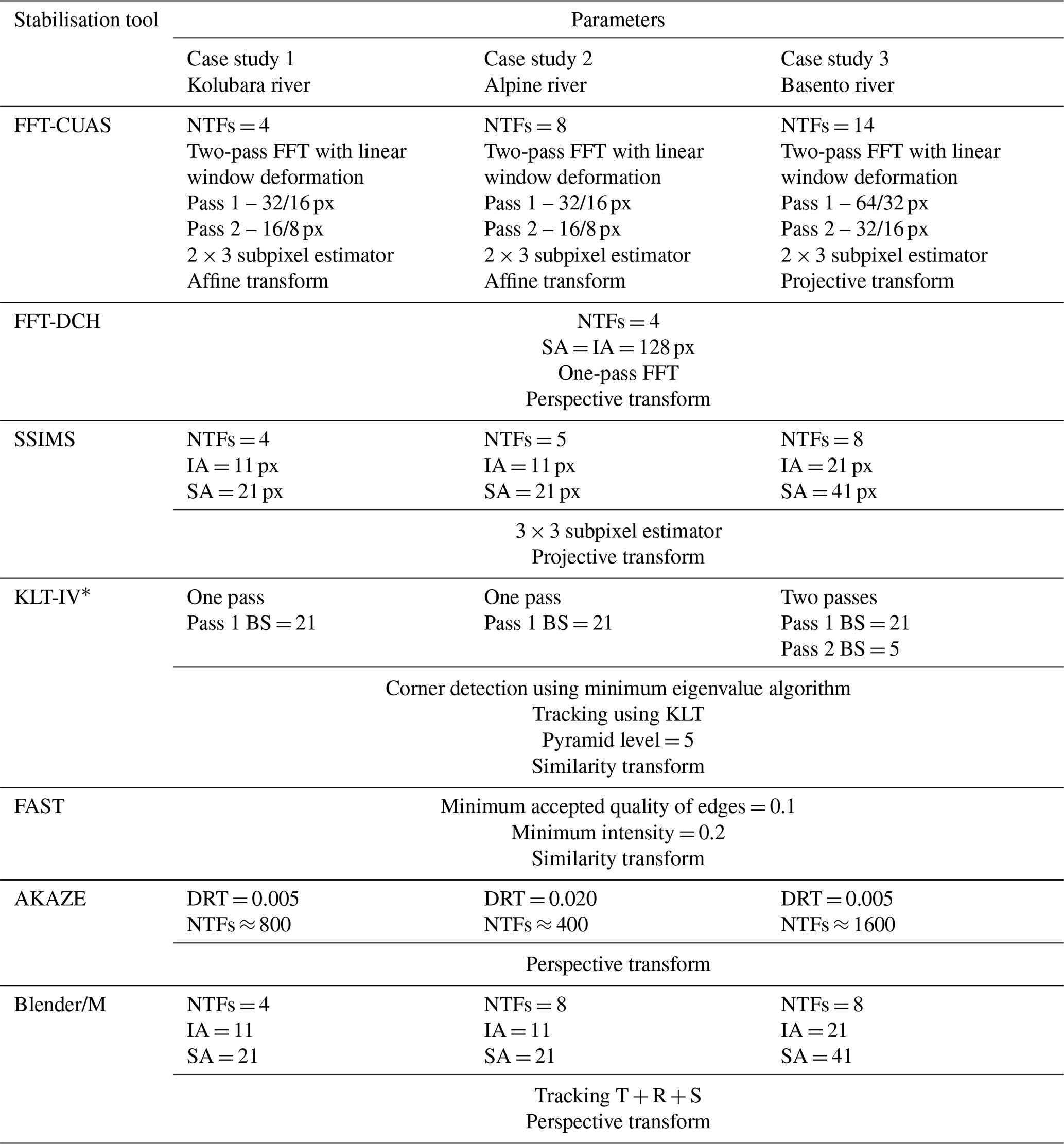
NTFs – number of tracked features; IA – interrogation area size; SA – search area size; DRT – detector response threshold; BS – block size (or search area size); T + R + S is translation + rotation + scaling of features. ∗ Only the number of passes can be adjusted; all other settings are default.
Table A2Polynomial fit coefficients and coefficients of determination for the d(RMSD) relationships.

Table A3Locations of repositories for the stabilisation tools with versions used in this study (as of 21 February 2021), along with the location of the data set containing unstabilised and stabilised frames from all three case studies.
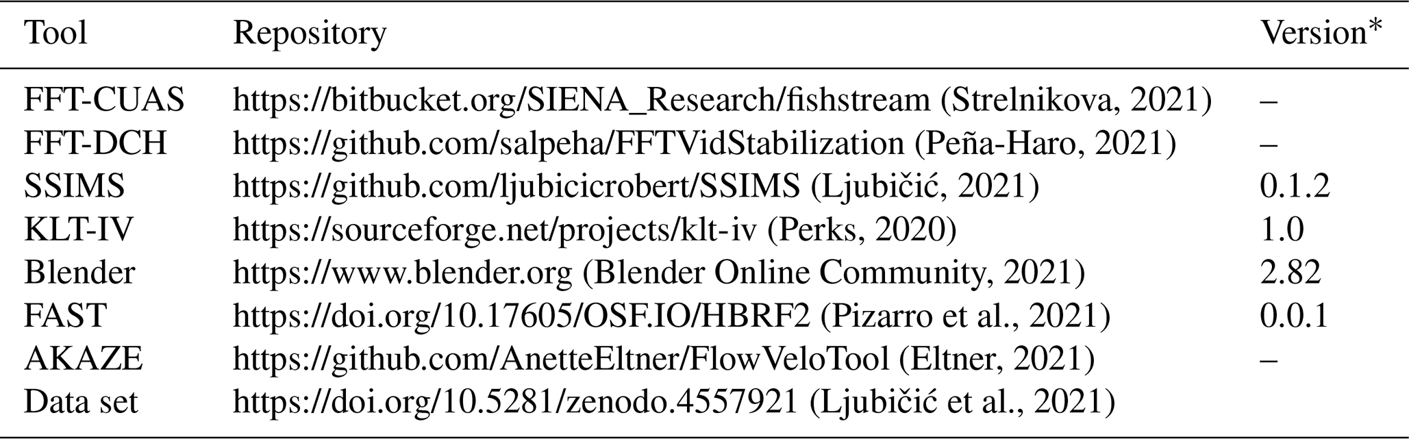
∗ Some tools do not use versions.
Models and data sets are shown in Table A3.
The supplement related to this article is available online at: https://doi.org/10.5194/hess-25-5105-2021-supplement.
The research was conceptualised by SM, SFDS, and AP. Data collection was done by US, SFDS, AP, and SM. RL and DS developed the methodology, performed formal analyses, wrote the original draft, and provided the visualisation. The software/algorithm implementations were written and developed by RL (SSIMS), DS (FFT-CUAS), MTP (KLT-IV), AE (AKAZE), SPH (FFT-DCH), and AP (FAST). The paper was reviewed and edited by MTP, AE, AP, SFDS, SPH, and SM. Supervision was provided by SM and MP. Funding and project administration was provided by SM.
The authors declare that they have no conflict of interest.
Publisher's note: Copernicus Publications remains neutral with regard to jurisdictional claims in published maps and institutional affiliations.
This research has been supported by the European Cooperation in Science and Technology (COST Action; grant no. CA16219; “HARMONIOUS – Harmonization of UAS techniques for agricultural and natural ecosystems monitoring”).
This paper was edited by Giuliano Di Baldassarre and reviewed by two anonymous referees.
Abdullah, L. M., Tahir, N. M., and Samad, M.: Video stabilization based on point feature matching technique, Proc. – 2012 IEEE Control Syst. Grad. Res. Colloquium, ICSGRC 2012, (Icsgrc), 303–307, https://doi.org/10.1109/ICSGRC.2012.6287181, 2012.
Aguilar, W. G. and Angulo, C.: Real-time video stabilization without phantom movements for micro aerial vehicles, Eurasip J. Image Video Process., 2014, 1–13, https://doi.org/10.1186/1687-5281-2014-46, 2014a.
Aguilar, W. G. and Angulo, C.: Robust video stabilization based on motion intention for low-cost micro aerial vehicles, 2014 IEEE 11th Int. Multi-Conference Syst. Signals Devices, SSD 2014, 1–6, https://doi.org/10.1109/SSD.2014.6808863, 2014b.
Aguilar, W. G. and Angulo, C.: Real-Time Model-Based Video Stabilization for Microaerial Vehicles, Neural Process. Lett., 43, 459–477, https://doi.org/10.1007/s11063-015-9439-0, 2016.
Alcantarilla, P., Nuevo, J., and Bartoli, A.: Fast Explicit Diffusion for Accelerated Features in Nonlinear Scale Spaces, in Procedings of the British Machine Vision Conference 2013, British Machine Vision Association, 13.1–13.11, https://doi.org/10.5244/C.27.13, 2013.
Auysakul, J., Xu, H., and Pooneeth, V.: A hybrid motion estimation for video stabilization based on an IMU sensor, Sensors (Switzerland), 18, 2708, https://doi.org/10.3390/s18082708, 2018.
Baek, D., Seo, I. W., Kim, J. S., and Nelson, J. M.: UAV-based measurements of spatio-temporal concentration distributions of fluorescent tracers in open channel flows, Adv. Water Resour., 127, 76–88, https://doi.org/10.1016/j.advwatres.2019.03.007, 2019.
Battiato, S., Gallo, G., Puglisi, G., and Scellato, S.: SIFT Features Tracking for Video Stabilization, in 14th International Conference on Image Analysis and Processing (ICIAP 2007), IEEE, 825–830, https://doi.org/10.1109/ICIAP.2007.4362878, 2007.
Battiato, S., Puglisi, G., and Bruna, A. R.: A robust video stabilization system by adaptive motion vectors filtering, in 2008 IEEE International Conference on Multimedia and Expo, IEEE, 373–376, https://doi.org/10.1109/ICME.2008.4607449, 2008.
Batur, A. U. and Flinchbaugh, B.: Video stabilization with optimized motion estimation resolution, Proc. – Int. Conf. Image Process. ICIP, 465–468, https://doi.org/10.1109/ICIP.2006.312494, 2006.
Blender Online Community: Blender – a 3D modelling and rendering package, Stichting Blender Foundation, Amsterdam, available at: https://www.blender.org, last access: 21 February 2021.
Censi, A., Fusiello, A., and Roberto, V.: Image stabilization by features tracking, Proc. – Int. Conf. Image Anal. Process. ICIAP 1999, 1, 665–669, https://doi.org/10.1109/ICIAP.1999.797671, 1999.
Chang, H.-C., Lai, S.-H., and Lu, K.-R.: A robust and efficient video stabilization algorithm, in IEEE International Conference on Multimedia and Expo (ICME), IEEE Cat. No.04TH8763, IEEE, 29–32, https://doi.org/10.1109/ICME.2004.1394117, 2004.
Choi, S., Kim, T., and Yu, W.: Robust video stabilization to outlier motion using adaptive RANSAC, in 2009 IEEE/RSJ International Conference on Intelligent Robots and Systems, IEEE, 1897–1902, https://doi.org/10.1109/IROS.2009.5354240, 2009.
Dal Sasso, S. F., Pizarro, A., and Manfreda, S.: Metrics for the Quantification of Seeding Characteristics to Enhance Image Velocimetry Performance in Rivers, Remote Sens., 12, 1789, https://doi.org/10.3390/rs12111789, 2020.
Deng, Z., Yang, D., Zhang, X., Dong, Y., Liu, C., and Shen, Q.: Real-Time Image Stabilization Method Based on Optical Flow and Binary Point Feature Matching, Electronics, 9, 198, https://doi.org/10.3390/electronics9010198, 2020.
Detert, M. and Weitbrecht, V.: Helicopter-based surface PIV experiments at Thur River, in River Flow 2014, CRC Press, 2003–2008, https://doi.org/10.1201/b17133-267, 2014.
Detert, M. and Weitbrecht, V.: A low-cost airborne velocimetry system: Proof of concept, J. Hydraul. Res., 53, 532–539, https://doi.org/10.1080/00221686.2015.1054322, 2015.
Detert, M., Johnson, E. D., and Weitbrecht, V.: Proof-of-concept for low-cost and non-contact synoptic airborne river flow measurements, Int. J. Remote Sens., 38, 2780–2807, https://doi.org/10.1080/01431161.2017.1294782, 2017.
Eltner, A.: FlowVeloTool, GitHub [code], available at: https://github.com/AnetteEltner/FlowVeloTool, last access: 21 February 2021.
Eltner, A., Sardemann, H., and Grundmann, J.: Technical Note: Flow velocity and discharge measurement in rivers using terrestrial and unmanned-aerial-vehicle imagery, Hydrol. Earth Syst. Sci., 24, 1429–1445, https://doi.org/10.5194/hess-24-1429-2020, 2020.
Engelsberg, A. and Schmidt, G.: A comparative review of digital image stabilising algorithms for mobile video communications, in Digest of Technical Papers. International Conference on Consumer Electronics (Cat. No.99CH36277), IEEE, 88–89, https://doi.org/10.1109/ICCE.1999.785180, 1999.
Ertürk, S.: Real-time digital image stabilization using Kalman filters, Real-Time Imaging, 8, 317–328, https://doi.org/10.1006/rtim.2001.0278, 2002.
Ertürk, S.: Digital image stabilization with sub-image phase correlation based global motion estimation, IEEE Trans. Consum. Electron., 49, 1320–1325, https://doi.org/10.1109/TCE.2003.1261235, 2003.
Fischler, M. A. and Bolles, R. C.: Random sample consensus: a paradigm for model fitting with applications to image analysis and automated cartography, Commun. ACM, 24, 381–395, https://doi.org/10.1145/358669.358692, 1981.
Fujita, I. and Notoya, Y.: Development of Uav-Based River Surface Velocity Measurement By Stiv Based on High-Accurate Image Stabilization Techniques, E-proceedings 36th IAHR World Congr., 28 June–3 July 2015, Hague, Netherlands Dev., 1, 1–10, 2015.
Grundmann, M., Kwatra, V., and Essa, I.: Auto-directed video stabilization with robust L1 optimal camera paths, in: CVPR 2011, IEEE, 225–232, https://doi.org/10.1109/CVPR.2011.5995525, 2011.
Hanning, G., Forslow, N., Forssen, P.-E., Ringaby, E., Tornqvist, D., and Callmer, J.: Stabilizing cell phone video using inertial measurement sensors, in 2011 IEEE International Conference on Computer Vision Workshops (ICCV Workshops), IEEE, 1–8, https://doi.org/10.1109/ICCVW.2011.6130215, 2011.
Hong, S., Hong, T., and Yang, W.: Multi-resolution unmanned aerial vehicle video stabilization, Proc. IEEE 2010 Natl. Aerosp. Electron. Conf. NAECON 2010, 126–131, https://doi.org/10.1109/NAECON.2010.5712935, 2010.
Hu, R., Shi, R., Shen, I. F., and Chen, W.: Video stabilization using scale-invariant features, Proc. Int. Conf. Inf. Vis., 871–876, https://doi.org/10.1109/IV.2007.119, 2007.
Kejriwal, L. and Singh, I.: A Hybrid Filtering Approach of Digital Video Stabilization for UAV Using Kalman and Low Pass Filter, Procedia Comput. Sci., 93, 359–366, https://doi.org/10.1016/j.procs.2016.07.221, 2016.
Kwon, O., Shin, J., and Paik, J.: Video stabilization using Kalman filter and phase correlation matching, Lect. Notes Comput. Sci. (including Subser. Lect. Notes Artif. Intell. Lect. Notes Bioinformatics), 3656 LNCS, 141–148, https://doi.org/10.1007/11559573_18, 2005.
Le Boursicaud, R., Pénard, L., Hauet, A., Thollet, F., and Le Coz, J.: Gauging extreme floods on YouTube: application of LSPIV to home movies for the post-event determination of stream discharges, Hydrol. Process., 30, 90–105, https://doi.org/10.1002/hyp.10532, 2016.
Le Coz, J., Patalano, A., Collins, D., Guillén, N. F., Garciá, C. M., Smart, G. M., Bind, J., Chiaverini, A., Le Boursicaud, R., Dramais, G., and Braud, I.: Lessons learnt from recent citizen science initiatives to document floods in France, Argentina and New Zealand, E3S Web Conf., 7, 6–11, https://doi.org/10.1051/e3sconf/20160716001, 2016.
Lewis, Q. W., Lindroth, E. M., and Rhoads, B. L.: Integrating unmanned aerial systems and LSPIV for rapid, cost-effective stream gauging, J. Hydrol., 560, 230–246, https://doi.org/10.1016/j.jhydrol.2018.03.008, 2018.
Liberzon, A., Lasagna, D., Aubert, M., Bachant, P., Mahmoodtabar, E., Käufer, T., jakirkham, Bauer, A., Vodenicharski, B., Dallas, C., Yang, E., Borg, J., Farzan, M. M., tomerast and ranleu: OpenPIV/openpiv-python: OpenPIV-Python v0.22.3, Zenodo, https://doi.org/10.5281/ZENODO.4042115, 2020.
Lim, A., Ramesh, B., Yang, Y., Xiang, C., Gao, Z., and Lin, F.: Real-time optical flow-based video stabilization for unmanned aerial vehicles, J. Real-Time Image Process., 16, 1975–1985, https://doi.org/10.1007/s11554-017-0699-y, 2019.
Litvin, A., Konrad, J., and Karl, W. C.: Probabilistic video stabilization using Kalman filtering and mosaicing, Image Video Commun. Process. 2003, 5022, 663, https://doi.org/10.1117/12.476436, 2003.
Liu, F., Gleicher, M., Jin, H., and Agarwala, A.: Content-preserving warps for 3D video stabilization, ACM Trans. Graph., 28, 1–9, https://doi.org/10.1145/1531326.1531350, 2009.
Liu, F., Gleicher, M., Wang, J., Jin, H., and Agarwala, A.: Subspace video stabilization, ACM Trans. Graph., 30, 4, https://doi.org/10.1145/1899404.1899408, 2011.
Liu, S., Wang, Y., Yuan, L., Bu, J., Tan, P., and Sun, J.: Video stabilization with a depth camera, in: 2012 IEEE Conference on Computer Vision and Pattern Recognition, IEEE, 89–95, https://doi.org/10.1109/CVPR.2012.6247662, 2012.
Liu, S., Yuan, L., Tan, P., and Sun, J.: Bundled camera paths for video stabilization, ACM Trans. Graph., 32, 78, https://doi.org/10.1145/2461912.2461995, 2013.
Ljubičić, R.: SSIMS: SSIM-based digital image stabilization suite, GitHub [code], available at: https://github.com/ljubicicrobert/SSIMS, last access: 21 February 2021.
Ljubičić, R., Strelnikova, D., Perks, M. T., Eltner, A., Peña-Haro, S., Pizarro, A., Dal Sasso, S. F., Scherling, U., Vuono, P., and Manfreda, S.: Video stabilisation results obtained using different tools for UAS-based image velocimetry (v1.0), Zenodo [data set], https://doi.org/10.5281/zenodo.4557921, 2021.
Lowe, D. G.: Distinctive Image Features from Scale-Invariant Keypoints, Int. J. Comput. Vis., 60, 91–110, https://doi.org/10.1023/B:VISI.0000029664.99615.94, 2004.
Mai, Y., Zhao, H., and Guo, S.: The analysis of image stabilization technology based on small-UAV airborne video, Proc. – 2012 Int. Conf. Comput. Sci. Electron. Eng. ICCSEE 2012, 3, 586–589, https://doi.org/10.1109/ICCSEE.2012.77, 2012.
Manfreda, S., McCabe, M., Miller, P., Lucas, R., Pajuelo Madrigal, V., Mallinis, G., Ben Dor, E., Helman, D., Estes, L., Ciraolo, G., Müllerová, J., Tauro, F., de Lima, M., de Lima, J., Maltese, A., Frances, F., Caylor, K., Kohv, M., Perks, M., Ruiz-Pérez, G., Su, Z., Vico, G., and Toth, B.: On the Use of Unmanned Aerial Systems for Environmental Monitoring, Remote Sens., 10, 641, https://doi.org/10.3390/rs10040641, 2018.
Manfreda, S., Dal Sasso, S. F., Pizarro, A., and Tauro, F.: Chapter 10: New Insights Offered by UAS for River Monitoring, in Applications of Small Unmanned Aircraft Systems: Best Practices and Case Studies, CRC Press, Taylor & Francis Grous, 2019.
Marcenaro, L., Vernazza, G., and Regazzoni, C. S.: Image stabilization algorithms for video-surveillance applications, in Proceedings 2001 International Conference on Image Processing (Cat. No.01CH37205), IEEE, 1, 349–352, https://doi.org/10.1109/ICIP.2001.959025, 2001.
MathWorks: What Is Camera Calibration?, available at: https://www.mathworks.com/help/vision/ug/camera-calibration.html, last access: 19 May 2021a.
MathWorks: Camera Calibrator, available at: https://www.mathworks.com/help/vision/ug/single-camera-calibrator-app.html, last access: 19 May 2021b.
Matsushita, Y., Ofek, E., Tang, X., and Shum, H. Y.: Full-frame video stabilization, Proc. – 2005 IEEE Comput. Soc. Conf. Comput. Vis. Pattern Recognition, CVPR 2005, I, 50–57, https://doi.org/10.1109/CVPR.2005.166, 2005.
Morimoto, C. and Chellappa, R.: Fast electronic digital image stabilization, Proc. – Int. Conf. Pattern Recognit., 3, 284–288, https://doi.org/10.1109/ICPR.1996.546956, 1996a.
Morimoto, C. and Chellappa, R.: Fast Electronic Digital Image Stabilization for Off-Road Navigation, Real-Time Imaging, 2, 285–296, https://doi.org/10.1006/rtim.1996.0030, 1996b.
Morimoto, C. and Chellappa, R.: Evaluation of image stabilization algorithms, in: Proceedings of the 1998 IEEE International Conference on Acoustics, Speech and Signal Processing, ICASSP '98 (Cat. No.98CH36181), IEEE, 5, 2789–2792, https://doi.org/10.1109/ICASSP.1998.678102, 1998.
Niskanen, M., Silven, O., and Tico, M.: Video Stabilization Performance Assessment, in 2006 IEEE International Conference on Multimedia and Expo, IEEE, 405–408, https://doi.org/10.1109/ICME.2006.262522, 2006.
Odelga, M., Kochanek, N., and Bülthoff, H. H.: Efficient real-time video stabilization for UAVs using only IMU data, 2017 Workshop on Research, Education and Development of Unmanned Aerial Systems (RED-UAS), 210–215, https://doi.org/10.1109/RED-UAS.2017.8101668, 2017.
OpenCV: Camera calibration With OpenCV, Open Source Computer Vision, available at: https://docs.opencv.org/master/d4/d94/tutorial_camera_calibration.html, last access: 19 May 2021.
Pearce, S., Ljubičić, R., Peña-Haro, S., Perks, M., Tauro, F., Pizarro, A., Dal Sasso, S., Strelnikova, D., Grimaldi, S., Maddock, I., Paulus, G., Plavšić, J., Prodanović, D., and Manfreda, S.: An Evaluation of Image Velocimetry Techniques under Low Flow Conditions and High Seeding Densities Using Unmanned Aerial Systems, Remote Sens., 12, 232, https://doi.org/10.3390/rs12020232, 2020.
Peña-Haro, S.: FFTVidStabilization, GitHub [code], available at: https://github.com/salpeha/FFTVidStabilization, last access: 21 February 2021.
Perks, M. T.: KLT-IV v1.0: image velocimetry software for use with fixed and mobile platforms, Geosci. Model Dev., 13, 6111–6130, https://doi.org/10.5194/gmd-13-6111-2020, 2020.
Perks, M. T.: KLT-IV, SourceForge [code], available at: https://sourceforge.net/projects/klt-iv (last access: 21 February 2021), 2020.
Perks, M. T., Russell, A. J., and Large, A. R. G.: Technical Note: Advances in flash flood monitoring using unmanned aerial vehicles (UAVs), Hydrol. Earth Syst. Sci., 20, 4005–4015, https://doi.org/10.5194/hess-20-4005-2016, 2016.
Pinto, B. and Anurenjan, P. R.: Video stabilization using Speeded Up Robust Features, ICCSP 2011–2011 Int. Conf. Commun. Signal Process., 527–531, https://doi.org/10.1109/ICCSP.2011.5739378, 2011.
Pizarro, A., Dal Sasso, S. F., Perks, M. T., and Manfreda, S.: Identifying the optimal spatial distribution of tracers for optical sensing of stream surface flow, Hydrol. Earth Syst. Sci., 24, 5173–5185, https://doi.org/10.5194/hess-24-5173-2020, 2020.
Pizarro, A., Dal Sasso, S. F., and Manfreda, S.: VISION: VIdeo StabilisatION using automatic features selection, OSF [code], https://doi.org/10.17605/OSF.IO/HBRF2, 2021.
Puglisi, G. and Battiato, S.: A robust image alignment algorithm for video stabilization purposes, IEEE Trans. Circuits Syst. Video Technol., 21, 1390–1400, https://doi.org/10.1109/TCSVT.2011.2162689, 2011.
Rosten, E. and Drummond, T.: Machine Learning for High-Speed Corner Detection, in: Leonardis, A., Bischof, H., and Pinz, A., Computer Vision – ECCV 2006, ECCV 2006, Lecture Notes in Computer Science, vol 3951, Springer, Berlin, Heidelberg, https://doi.org/10.1007/11744023_34, 2006.
Shen, H., Pan, Q., Cheng, Y., and Yu, Y.: Fast video stabilization algorithm for UAV, in IEEE International Conference on Intelligent Computing and Intelligent Systems, IEEE, 542–546, https://doi.org/10.1109/ICICISYS.2009.5357609, 2009.
Shi, J. and Tomasi, C.: Good features to track, in Proceedings of IEEE Conference on Computer Vision and Pattern Recognition CVPR-94, IEEE Comput. Soc. Press, 593–600, https://doi.org/10.1109/CVPR.1994.323794, 1994.
Stegagno, P., Basile, M., Bulthoff, H. H., and Franchi, A.: A semi-autonomous UAV platform for indoor remote operation with visual and haptic feedback, in: 2014 IEEE International Conference on Robotics and Automation (ICRA), IEEE, 3862–3869, https://doi.org/10.1109/ICRA.2014.6907419, 2014.
Strelnikova, D.: Fishstream: Extended PiVlab version with the FFT_CUAS stabilisation tool, Bitbucket [code], available at: https://bitbucket.org/SIENA_Research/fishstream, last access: 21 February 2021.
Strelnikova, D., Paulus, G., Käfer, S., Anders, K.-H., Mayr, P., Mader, H., Scherling, U., and Schneeberger, R.: Drone-Based Optical Measurements of Heterogeneous Surface Velocity Fields around Fish Passages at Hydropower Dams, Remote Sens., 12, 384, https://doi.org/10.3390/rs12030384, 2020.
Tauro, F., Porfiri, M., and Grimaldi, S.: Surface flow measurements from drones, J. Hydrol., 540, 240–245, https://doi.org/10.1016/j.jhydrol.2016.06.012, 2016.
Thielicke, W. and Stamhuis, E. J.: PIVlab – Towards User-friendly, Affordable and Accurate Digital Particle Image Velocimetry in MATLAB, J. Open Res. Softw., 2, e30, https://doi.org/10.5334/jors.bl, 2014.
Thillainayagi, R. and Senthil Kumar, K.: Video stabilization technique for thermal infrared Aerial surveillance, Online International Conference on Green Engineering and Technologies (IC-GET), 2016, https://doi.org/10.1109/GET.2016.7916630, 2016.
Wang, Y., Hou, Z. J., Leman, K., and Chang, R.: Real-time video stabilization for Unmanned Aerial Vehicles, Proc. 12th IAPR Conf. Mach. Vis. Appl. MVA 2011, 336–339, 2011.
Wang, Z., Bovik, A. C., Sheikh, H. R., and Simoncelli, E. P.: Image Quality Assessment: From Error Visibility to Structural Similarity, IEEE Trans. Image Process., 13, 600–612, https://doi.org/10.1109/TIP.2003.819861, 2004.
Yang, J., Schonfeld, D., and Mohamed, M.: Robust video stabilization based on particle filter tracking of projected camera motion, IEEE Trans. Circuits Syst. Video Technol., 19, 945–954, https://doi.org/10.1109/TCSVT.2009.2020252, 2009.