Reduction of vegetation-accessible water storage capacity after deforestation affects catchment travel time distributions and increases young water fractions in a headwater catchment

Deforestation can considerably affect transpiration dynamics and magnitudes at the catchment scale and thereby alter the partitioning between drainage and evaporative water fluxes released from terrestrial hydrological systems. However, it has so far remained problematic to directly link reductions in transpiration to changes in the physical properties of the system and to quantify these changes in system properties at the catchment scale. As a consequence, it is difficult to quantify the effect of deforestation on parameters of catchment-scale hydrological models. This in turn leads to substantial uncertainties in predictions of the hydrological response after deforestation but also to a poor understanding of how deforestation affects principal descriptors of catchment-scale transport, such as travel time distributions and young water fractions. The objectives of this study in the Wüstebach experimental catchment are therefore to provide a mechanistic explanation of why changes in the partitioning of water fluxes can be observed after deforestation and how this further affects the storage and release dynamics of water. More specifically, we test the hypotheses that (1) post-deforestation changes in water storage dynamics and partitioning of water fluxes are largely a direct consequence of a reduction of the catchment-scale effective vegetation-accessible water storage capacity in the unsaturated root zone (S_U, max) after deforestation and that (2) the deforestation-induced reduction of S_U, max affects the shape of travel time distributions and results in shifts towards higher fractions of young water in the stream. Simultaneously modelling streamflow and stable water isotope dynamics using meaningfully adjusted model parameters both for the pre- and post-deforestation periods, respectively, a hydrological model with an integrated tracer routine based on the concept of storage-age selection functions is used to track fluxes through the system and to estimate the effects of deforestation on catchment travel time distributions and young water fractions F_yw.

It was found that deforestation led to a significant increase in streamflow accompanied by corresponding reductions of evaporative fluxes. This is reflected by an increase in the runoff ratio from C_R=0.55 to 0.68 in the post-deforestation period despite similar climatic conditions. This reduction of evaporative fluxes could be linked to a reduction of the catchment-scale water storage volume in the unsaturated soil (S_U, max) that is within the reach of active roots and thus accessible for vegetation transpiration from ∼258 mm in the pre-deforestation period to ∼101 mm in the post-deforestation period. The hydrological model, reflecting the changes in the parameter S_U, max, indicated that in the post-deforestation period stream water was characterized by slightly yet statistically not significantly higher mean fractions of young water (F_yw∼0.13) than in the pre-deforestation period (F_yw∼0.12). In spite of these limited effects on the overall F_yw, changes were found for wet periods, during which post-deforestation fractions of young water increased to values F_yw∼0.37 for individual storms. Deforestation also caused a significantly increased sensitivity of young water fractions to discharge under wet conditions from $\mathrm{d}{F}_{\text{yw}}/\mathrm{d}Q=\mathrm{0.25}$ to 0.36.

Overall, this study provides quantitative evidence that deforestation resulted in changes in vegetation-accessible storage volumes S_U, max and that these changes are not only responsible for changes in the partitioning between drainage and evaporation and thus the fundamental hydrological response characteristics of the Wüstebach catchment, but also for changes in catchment-scale tracer circulation dynamics. In particular for wet conditions, deforestation caused higher proportions of younger water to reach the stream, implying faster routing of stable isotopes and plausibly also solutes through the sub-surface.

1 Introduction

Plant transpiration is, globally, the largest continental water flux (Jasechko, 2018). Notwithstanding considerable uncertainties (Coenders-Gerrits, 2014), its magnitude depends on the interplay between canopy water demand and sub-surface water supply (Eagleson, 1982; Milly and Dunne, 1994; Donohue et al., 2007; Yang et al., 2016; Jaramillo et al., 2018; Mianabadi et al., 2019). The latter is regulated by water volumes that are within the reach of roots and can be taken up by plants. Many plant species across humid climate zones develop only rather shallow root systems (Schenk, 2005) that do not directly tap the groundwater (Fan et al., 2017). In regions that are dominated by such shallow-rooting vegetation, the pore volume between field capacity and permanent wilting point that is within the reach of active roots becomes a core property of many terrestrial hydrological systems (Rodriguez-Iturbe et al., 2007). This maximum vegetation-accessible water storage volume in the unsaturated root zone of soils, hereafter referred to as vegetation-accessible water storage capacity S_U, max (mm), constitutes a major partitioning point of water fluxes. It regulates the temporally varying ratio between drainage, such as groundwater recharge or shallow lateral flow on the one hand and transpiration fluxes on the other hand (Savenije and Hrachowitz, 2017), which can in turn generate considerable feedback effects on downwind precipitation and drought generation (e.g. Seneviratne et al., 2013; Ellison et al., 2017; Teuling, 2018; Wang-Erlandsson et al., 2018; Wehrli et al., 2019).

Traditionally, S_U, max is determined as the product of root depths or root distributions and porewater content between field capacity and permanent wilting point. Although correct in principle, this method has several weaknesses for applications at the catchment scale as much of the required data are typically not available at sufficient levels of detail. While soil maps and the associated soil water retention curves have become globally available at resolutions <1 km (Arrouays et al., 2017; Hengl et al., 2017), they are characterized by considerable uncertainties. Similarly, direct and detailed observations of root systems are very scarce. They are, globally, limited to a few thousand individual plants only (e.g. Schenk and Jackson, 2002; Fan et al., 2017), and many of the observations are based on biomass extrapolations after excavating only the first metre of soil or less (Schenk and Jackson, 2003). Consequently, soil and root data largely remain inaccurate snapshots in space. As such, they are likely to be inadequate reflections of the spatial heterogeneity of soils and roots. In addition, these available data are also mostly snapshots in time and therefore disregard the adaptive behaviour of plant communities, whose compositions, and thus characteristics, at ecosystem level continuously evolve over multiple scales in space and time in response to changes in ambient conditions (e.g. Laio et al., 2006; Brunner et al., 2015; Tron et al., 2015).

There is increasing evidence that vegetation does not only actively adapt to its (changing) environment, but that it also does so in a way that allows the most efficient use of available energy and resources (e.g. Guswa, 2008; Schymanski et al., 2008). The vegetation, i.e. a collective of individual different plants within an area of interest that is present at any given moment at any given location, has survived past conditions. This in itself is a manifestation of the successful adaption of individual plants to their environment in the past. They have optimally allocated resources to balance sub- and above-surface growth to simultaneously meet water, nutrient and light requirements. This implies that these plants developed root systems that, amongst other factors, ensure continuous access to sufficient water – but not more – to bridge dry periods. An individual plant that is not adapted to meet its water and nutrient requirements through its root system as well as its light requirements through its foliage system in competition with other plants will disappear and be replaced by a better adapted plant. The root system of vegetation at ecosystem level and the associated vegetation-accessible water storage capacity S_U, max are therefore at a dynamic equilibrium with and responding to the ever-changing conditions of its environment. Similarly, any type of direct human interference with vegetation, such as deforestation, has an impact on transpiration water demand, the extent and structure of active root systems and consequently on S_U, max (Nijzink et al., 2016a).

For a meaningful quantification of S_U, max at larger scales, such as the catchment scale, it is therefore necessary to adopt a Darwinian perspective (Harman and Troch, 2014) and to estimate effective values of S_U, max, reflecting the collective and adaptive behaviour of all individual plants within a catchment. Results from many previous studies suggest, broadly speaking, three methods to do so. The first is the use of inverse approaches that treat S_U, max as a model calibration parameter (Fenicia et al., 2008; Speich et al., 2018; Bouaziz et al., 2020; Knighton et al., 2020). Alternatively, the second type of method is based on optimality principles that maximize variables such as net primary production or carbon gain (Kleidon, 2004; Guswa, 2008; Hwang et al., 2009; Yang, et al., 2016; Speich et al., 2018, 2020), nitrogen uptake (McMurtrie et al., 2012) or transpiration rates (Collins and Bras, 2007; Sivandran and Bras, 2012). Lastly, S_U, max and its evolution over time can be directly estimated through magnitudes of annual water deficits as determined from observed water balance data (Gentine et al., 2012; Donohue et al., 2012; Gao et al., 2014; DeBoer-Euser et al., 2016; van Oorschot et al., 2021).

For transpiration, shallow-rooting plants extract porewater of unsaturated soils that is held against gravity, i.e. between field capacity and permanent wilting point, and within the reach of roots. Significant vertical or lateral drainage only occurs at water contents above field capacity. By extracting soil water below that, transpiration therefore generates a root-zone water storage reservoir between field capacity and permanent wilting point that is characterized by a storage capacity S_U, max, i.e. a maximum vegetation-accessible storage volume, and that is at any given moment filled with a specific water volume S_U(t), depending on the past sequence of water inflow and release.

Storage reservoirs such as S_U, max or others such as groundwater bodies are key for hydrological functioning (Sprenger et al., 2019b) as they provide a buffer against hydrological extremes such as floods and droughts. With larger storage reservoirs, the hydrological memory of a system can increase as more water can be stored and held over longer periods of time (e.g. Hrachowitz et al., 2015; Sprenger et al., 2019b). This also implies that while increased actual volumes of water stored in and thus the degree of filling of storage reservoirs, e.g. S_U(t), can reduce water ages (Harman, 2015), increased sizes of storage reservoirs, e.g. S_U, max, can increase water ages, both thereby controlling catchment travel time distributions (TTDs; Soulsby et al., 2010). As fundamental descriptors of hydrological functioning, TTDs describe the age structure of water held in and released from catchments (Birkel et al., 2015; Rinaldo et al., 2015), which is critical for regulating solute transport and thus nutrient and contaminant dynamics (Hrachowitz et al., 2016).

However, neither the effects of land cover change (Blöschl et al., 2019) nor the individual roles of different storage compartments in terrestrial hydrological systems are well understood (McDonnell et al., 2010; Penna et al., 2018, 2020). This is mostly a consequence of the lack of suitable observational technology to directly observe their respective volumes at larger scales. It remains therefore also unclear how deforestation affects S_U, max (e.g. due to a less developed and complex rooting system for subsequent younger vegetation) and how changes in S_U, max may propagate to affect both the partitioning of water fluxes as well as the age structure of water stored in and released from catchments as described by residence and travel time distributions.

For the study site of this paper, the Wüstebach experimental catchment (Germany), a previous study quantified the effects of deforestation on the partitioning of water fluxes (Wiekenkamp et al., 2016). It was found that forest removal significantly reduced evaporative fluxes. This led to more persistent higher soil moisture levels and eventually to increases in streamflow. Similarly, in the same catchment, Wiekenkamp et al. (2020) found evidence for increased post-deforestation occurrence of preferential flows, while Stockinger et al. (2019) reported minor post-deforestation reductions in travel times.

To establish a quantitative mechanistic link between these studies, we here aim to trace back and attribute the above-reported post-deforestation changes in the hydrological response of the Wüstebach to deforestation-induced changes in (sub-surface) system properties. The overall objective of this study is thus to analyse whether changes in these (sub-surface) properties can explain why deforestation affects water flux partitioning and reduces travel times in the Wüstebach in an attempt to improve our quantitative understanding of critical zone processes (Brooks et al., 2015). Specifically, we test the hypotheses that (1) post-deforestation changes in water storage dynamics and partitioning of water fluxes are largely a direct consequence of a reduction of the catchment-scale effective vegetation-accessible water storage capacity in the unsaturated root zone (S_U, max) after deforestation and that (2) the deforestation-induced reduction of S_U, max affects the shape of travel time distributions and results in shifts towards higher fractions of young water in the stream.

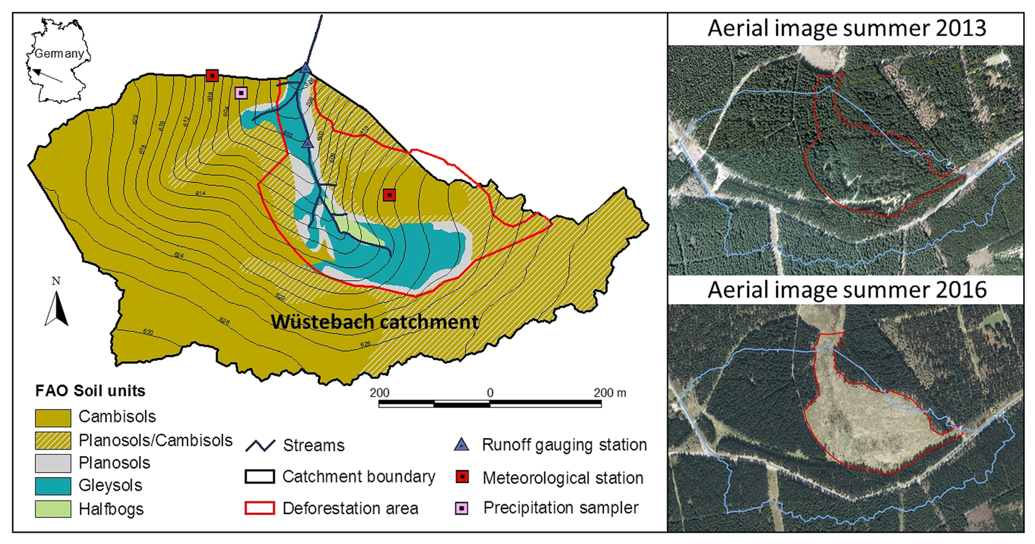
Figure 1 Map of the Wüstebach study catchment showing the spatial distribution of soil types. The riparian zone is defined by the parts of the catchment covered by Gleysols, Planosols and Halfbogs. The red line indicates the outline of the deforested part of the catchment, as can also be seen in the aerial images (© Google Earth, Maxar Technologies 2020) from 2013 and 2016.

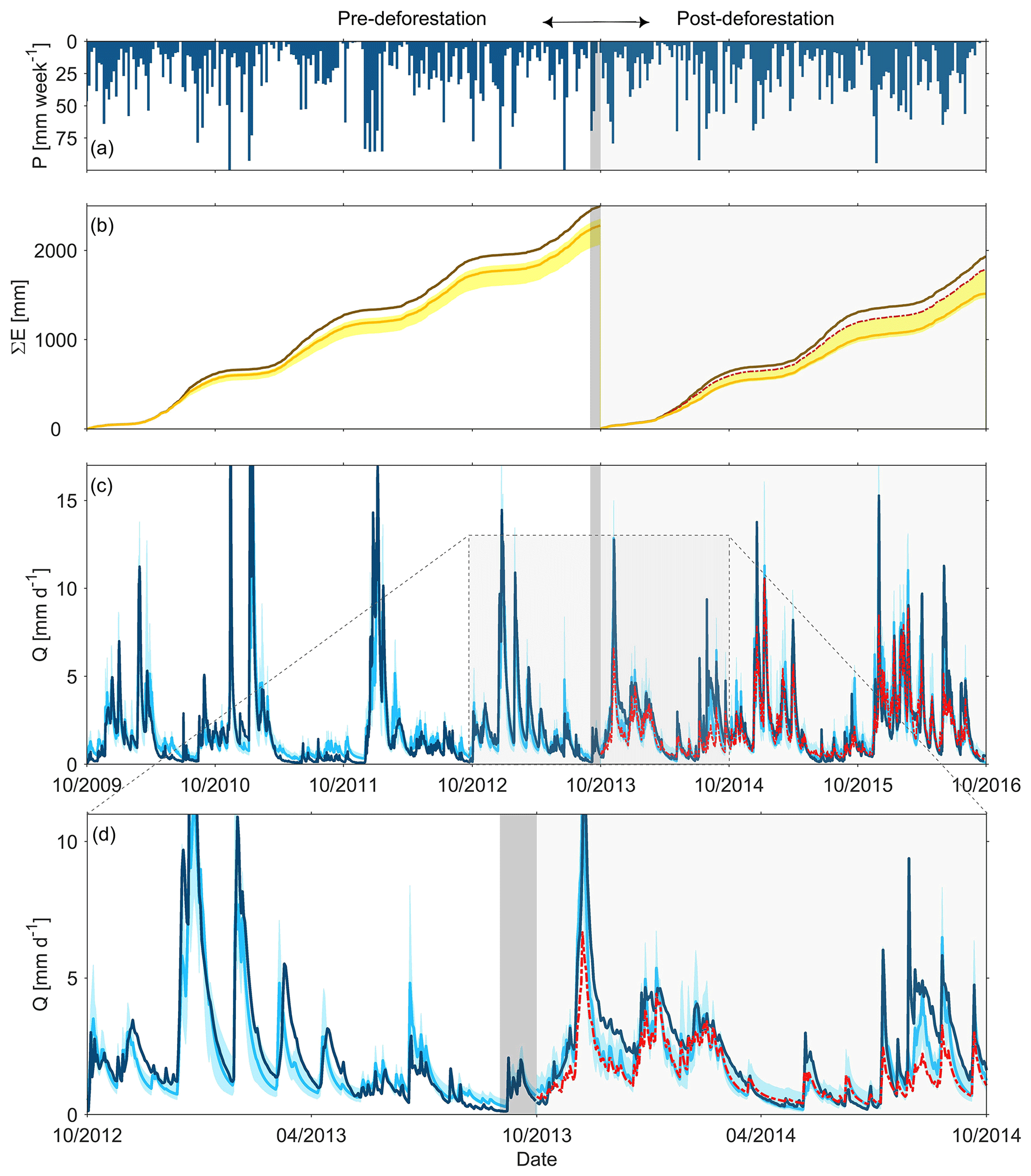
Figure 2 (a) Time series of observed weekly precipitation P; (b) daily cumulative evaporative fluxes for the pre- and post-deforestation periods, where the dark brown line indicates potential evaporation E_P and the orange lines and the yellow shaded areas show the actual evaporation E_A modelled using the best fit parameter sets and the associated 5th$/$95th percentiles of all feasible solutions of the pre- and post-deforestation periods, respectively. The dashed red line indicates the modelled E_A in the post-deforestation period using the best fit pre-deforestation parameter set; (c) observed (dark blue line) and modelled daily streamflow Q; light blue line indicates the best fit model and the shaded area the 5th$/$95th percentile of all feasible solutions for the pre- and post-deforestation periods, respectively. The dashed red line indicates the modelled streamflow in the post-deforestation period using the best fit pre-deforestation parameter set; (d) zoom-in to the observed and modelled streamflow for the October 2012–October 2014 period. The grey shaded area indicates the deforestation period.

2 Study site

The experimental Wüstebach headwater catchment (0.39 km²; Fig. 1a) is part of the Lower Rhine/Eifel Observatory of the Terrestrial Environmental Observatories network (TERENO; Bogena et al., 2018) located in the Eifel National Park in Germany (50^∘30'16” N, 06^∘20'00” E). The catchment is characterized by a humid, temperate climate with warm summers, mild winters and a mean annual temperature of around 7 ^∘C (Zacharias et al., 2011). Mean annual precipitation is about 1200 mm yr⁻¹ and mean annual runoff about 700 mm yr⁻¹ (Fig. 2). Although most of the precipitation occurs in the winter months, the fraction that falls as snow is typically less than 10 % of the annual precipitation, and snow cover is present for no more than 3–4 weeks per year.

The catchment is drained by a perennial second-order stream and extends from 595 to 630 $\mathrm{m}\mathrm{a}.\mathrm{s}.\mathrm{l}.$ The landscape is characterized by the gentle slopes of the surrounding hills and a flatter riparian area close to the stream, covering approximately 10 % of the catchment (Fig. 1a). The underlying bedrock is largely Devonian shales with sandstone inclusions (Richter, 2008) covered by periglacial layers (Borchardt, 2012). While Cambisols dominate the hillslopes, Gleysols and Histosols characterize much of the riparian area (Bogena et al., 2015). The average soil depth in the catchment reaches about 1.6 m with a maximum of 2 m (Graf et al., 2014). In 1946, after the Second World War, the catchment was homogeneously and completely afforested (Fig. 1) with Sitka spruce (Picea sitchensis) and Norway spruce (Picea abies; Etmann, 2009). The maximum observed rooting depth of these spruce trees in the catchment is 50 cm, and no roots were observed below this depth. In the course of the development of the area into a national park, approximately 21 % of the catchment, including the entire riparian zone, was deforested in September 2013 and has been kept largely vegetation free since (Wiekenkamp et al., 2016; Fig. 1).

3 Data

3.1 Hydro-meteorological data

Daily hydro-meteorological data were available for the period 1 October 2009–30 September 2016 (Fig. 2). Precipitation P (mm d⁻¹) and mean daily temperature T (^∘C) were available from the Monschau–Kalterherberg meteorological station operated by the German Weather Service (Deutscher Wetterdienst DWD station 3339), located 9 km north-west of the Wüstebach catchment. The precipitation data were corrected for evaporation and wind drift losses according to Richter (1995) and as described in detail by Graf et al. (2014). Stream discharge Q (mm d⁻¹) at the outlet of the Wüstebach was observed with a V-notch weir for low-flow measurements and a Parshall flume for medium to high flows (Bogena et al., 2015). Daily potential evaporation E_P (mm d⁻¹) was estimated using the Penman–Monteith equation. Daily depth-weighted average soil water content for the study period was estimated from a network of soil moisture sensors placed at 5, 20 and 50 cm depths at >100 locations across the study catchment as described by Graf et al. (2014) and Bogena et al. (2015). In addition, throughfall rates P_E (mm d⁻¹) were measured at one continuously forested location in the study catchment (Fig. 1) with an array of samplers as described in detail by Stockinger et al. (2015) over irregular intervals over the period 1 October 2012–30 September 2016.

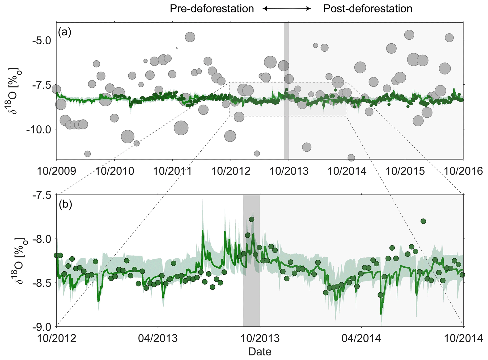
Figure 3 (a) Observed volume-weighted monthly δ¹⁸O signals in precipitation (grey dots; size of dots indicates the precipitation volume) and streamflow (green dots) as well as the best fit modelled δ¹⁸O signal in the stream (green line) and the 5th$/$95th percentile of all feasible solutions from pre- and post-deforestation calibration (green shaded area); (b) zoom-in of observed and modelled δ¹⁸O signals in the stream for the October 2012–October 2014 period.

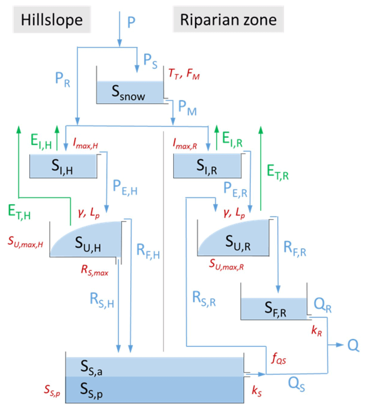
Figure 4 Model structure used in this study. The light blue boxes indicate the hydrologically active individual storage volumes in the hillslope and riparian zones, respectively. The darker blue box S_S,p indicates a hydrologically passive, i.e. $\mathrm{d}{S}_{\text{S,p}}/\mathrm{d}t=\mathrm{0}$, mixing volume. The blue lines indicate liquid water fluxes, and the green lines indicate vapour fluxes. Model parameters are shown in red adjacent to the model component they are associated with. All symbols are defined in Table 1.

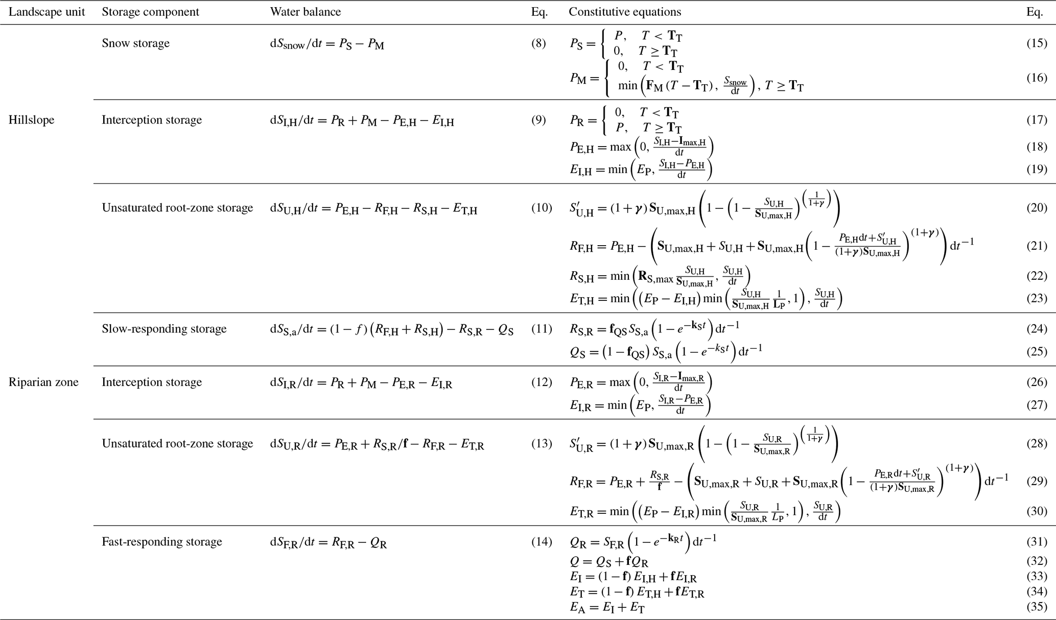
Table 1 Water balance, state and flux equations used in the hydrological model. Symbols shown in bold are model parameters. Subscripts H and R indicate hillslope and riparian zone, respectively. Model variables: P is total precipitation (mm d⁻¹), P_S is solid precipitation (snow) (mm d⁻¹), P_M is snowmelt (mm d⁻¹), P_R is rain (mm d⁻¹), P_E is throughfall (mm d⁻¹), E_P is potential evaporation (mm d⁻¹), E_I is interception evaporation (mm d⁻¹), R_F is preferential recharge (mm d⁻¹), R_S is slow recharge (mm d⁻¹), E_T is transpiration (mm d⁻¹), Q_S is flow from the slow-responding reservoir (mm d⁻¹), Q_R is flow from the fast-responding riparian reservoir (mm d⁻¹), Q is the total flow (mm d⁻¹) and E_A is the total actual evaporation (mm d⁻¹). Model parameters: T_T is the threshold temperature (^∘C), F_M is a melt factor ($\mathrm{mm}{\mathrm{d}}^{-\mathrm{1}}{}^{\circ }\mathrm{C}$⁻¹), I_max is the interception capacity (mm), S_U, max is the root-zone storage capacity (mm), γ is a shape factor (–), R_S,max is the maximum percolation rate (mm d⁻¹), L_p is a transpiration water stress factor (–), f_QS is a factor determining the fraction of groundwater flow that is upwelling into the riparian zone (–), k_S is the storage coefficient of the slow-responding reservoir (d⁻¹), k_R is the storage coefficient for the fast-responding riparian reservoir (d⁻¹) and f is the areal fraction of the riparian zone (–).

3.2 Stable isotope data

Regular weekly δ¹⁸O data from bulk precipitation samples collected in a cooled wet deposition gauge at the meteorological station Schleiden–Schöneseiffen (Meteomedia station) 3 km north-east of the catchment were available for the period 1 October 2010–24 September 2012. After that, precipitation was sampled at half-daily intervals until 30 September 2016 using an automatic, cooled sampler (Eigenbrodt GmbH, Germany). The half-daily samples were precipitation volume weighed to daily sampling intervals (Stockinger et al., 2016, 2017). Weekly stream water grab samples for stable water isotope analysis were taken at the outlet of the Wüstebach catchment in the 1 October 2010–30 September 2016 period (Fig. 3a; Bogena et al., 2020).

Isotope analysis was carried out using laser-based cavity ring-down spectrometers (L2120-i/L2130-i, Picarro Inc.). Internal standards calibrated against VSMOW, Greenland Ice Sheet Precipitation (GISP) and Standard Light Antarctic Precipitation (SLAP2) were used for calibration and to ensure long-term stability of analyses (Brand et al., 2014). The long-term precision of the analytical system was ≤0.1 % for δ¹⁸O.

4 Methods

To quantify effects of deforestation on S_U, max and, due to the role of S_U, max as a mixing volume also in the age structure of water as described by TTDs and the associated young water fractions F_yw, the following stepwise experiment was designed. (1) Quantify changes in the partitioning of annual water fluxes between the pre- and post-deforestation periods based on observed water balance data. (2) Estimate the effect of these changes on the magnitudes of pre- and post-deforestation S_U, max, respectively, using the same data. (3) Calibrate a hydrological model to simultaneously reproduce streamflow and stream δ¹⁸O dynamics for the pre-deforestation period. (4) Use the calibrated parameter sets to run the model in the post-deforestation period and evaluate the model's post-deforestation performance without further calibration. (5) Re-calibrate the model for the post-deforestation period and evaluate whether changes in calibrated S_U, max (and other parameters) are plausible and reflect changes in S_U, max directly estimated from water balance data in step (2). Finally, (6) use the calibrated pre- and post-deforestation parameter sets, respectively, to track modelled water fluxes through the system and quantify changes in TTDs and F_yw between the pre- and post-deforestation periods.

4.1 Water balance-based estimation of S_U, max

To survive, plants need continuous access to water to satisfy canopy water demand. The root systems of vegetation are therefore adapted to provide access to water volumes that correspond to annual water deficits that result from the combination of (1) the phase lag between and (2) the difference in the respective magnitudes of seasonal precipitation and solar radiation signals (Donohue et al., 2012; Gentine et al., 2012; Gao et al., 2014). On a daily basis, these water deficits S_D,j(t) can be estimated as the cumulative sum of daily throughfall P_E (mm d⁻¹) minus transpiration E_T (mm d⁻¹). The maximum deficit S_D,j for a specific year j is then equivalent to the soil water volume that was accessible to and actually accessed by vegetation through its root system for transpiration during the dry season over that period when E_T exceeded P_E (deBoer-Euser et al., 2016; Nijzink et al., 2016a; van Oorschot et al., 2021):

$$\begin{array}{}\text{(1)}& {\displaystyle }& {\displaystyle }{S}_{\mathrm{D},j}\left(t\right)=\left\{\begin{array}{ll}\underset{t_{\mathrm{0}}}{\overset{t}{\int }}\left(P_{\mathrm{E}}\left(t\right)-E_{\mathrm{T}}\left(t\right)\right)\mathrm{d}t,& \text{if }{S}_{\mathrm{D},j}\left(t\right)\le \mathrm{0},\\ \mathrm{0},& \text{if }{S}_{\mathrm{D},j}\left(t\right)>\mathrm{0},\end{array}\right.\text{(2)}& {\displaystyle }& {\displaystyle }{S}_{\mathrm{D},j}=max\left(\left|S_{\mathrm{D},j}\left(t\right)\right|\right),\end{array}$$

where t is the time step (d) and t₀ is the last preceding time step for which the storage deficit $S_{\mathrm{D},j}\left(t\right)=\mathrm{0}$. As an approximation, Eq. (1) implies that if $S_{\mathrm{D},j}\left(t\right)=\mathrm{0}$, the water content in the root-accessible pore space at day t is at field capacity and cannot hold additional water. If water supply then exceeds canopy water demand on that day, i.e. P_E(t)–E_T(t)>0, this water surplus is drained from the root zone, e.g. to recharge groundwater or directly to the stream, and cannot be used for transpiration.

Daily throughfall P_E, i.e. precipitation that actually reaches the soil, was estimated on the basis of the water balance of a canopy interception storage (Nijzink et al., 2016a):

$$\begin{array}{}\text{(3)}& {\displaystyle }{\displaystyle \frac{\mathrm{d}{S}_{\mathrm{I}}\left(t\right)}{\mathrm{d}t}}=P\left(t\right)-E_{\mathrm{I}}\left(t\right)-P_{\mathrm{E}}\left(t\right),\end{array}$$

where E_I (mm d⁻¹) is daily interception evaporation and S_I (mm) the canopy interception storage. For each time step, E_I can then be computed as

$$\begin{array}{}\text{(4)}& {\displaystyle }{\displaystyle }{E}_{\mathrm{I}}\left(t\right)=\left\{\begin{array}{ll}{E}_{\mathrm{P}}\left(t\right),& \text{if }{E}_{\mathrm{p}}\left(t\right)\mathrm{d}t<S_{\mathrm{I}}\left(t\right).\\ \frac{S_{\mathrm{I}}\left(t\right)}{\mathrm{d}t},& \text{if }{E}_{\mathrm{P}}\left(t\right)\mathrm{d}t\ge S_{\mathrm{I}}\left(t\right).\end{array}\right.\end{array}$$

This then further allows us to estimate P_E according to

$$\begin{array}{}\text{(5)}& {\displaystyle }{\displaystyle }{P}_{\mathrm{E}}\left(t\right)=\left\{\begin{array}{ll}\mathrm{0},& \text{if }{S}_{\mathrm{I}}\left(t\right)<I_{\text{max}},\\ \frac{S_{\mathrm{I}}\left(t\right)-I_{\text{max}}}{\mathrm{d}t},& \text{if }{S}_{\mathrm{I}}\left(t\right)\ge I_{\text{max}},\end{array}\right.\end{array}$$

where I_max (mm) is the canopy interception capacity. In the absence of more detailed information P_E was estimated with a range of different interception capacities, i.e. I_max=0, 1, 2, 3, and 4 mm, in a sensitivity analysis approach.

Note that the catchment average P_E after deforestation was estimated as the area-weighted mean of P_E in the deforested area (21 % of the catchment area) computed with an assumed I_max=0 mm and P_E from the remaining area computed based on the above range of I_max between 0 and 4 mm. In a next step, assuming negligible groundwater imports or exports (cf. Bouaziz et al., 2018), data errors and storage changes, long-term mean transpiration $\overline{E_{\mathrm{T}}}$ was estimated according to the water balance:

$$\begin{array}{}\text{(6)}& {\displaystyle }{\displaystyle }{\stackrel{\mathrm{‾}}{E}}_{\mathrm{T}}={\stackrel{\mathrm{‾}}{P}}_{\mathrm{E}}-\stackrel{\mathrm{‾}}{Q},\end{array}$$

where ${\stackrel{\mathrm{‾}}{P}}_{\mathrm{E}}$ (mm d⁻¹) is the long-term mean throughfall and $\stackrel{\mathrm{‾}}{Q}$ (mm d⁻¹) is the long-term mean observed stream discharge. Daily transpiration E_T (mm d⁻¹) for use in Eq. (1) is then estimated by scaling the long-term mean transpiration to the signal of daily potential evaporation to approximate the seasonal fluctuation of energy input (Bouaziz et al., 2020):

$$\begin{array}{}\text{(7)}& {\displaystyle }{\displaystyle }{E}_{\mathrm{T}}\left(t\right)=\left(E_{\mathrm{P}}\left(t\right)-E_{\mathrm{I}}\left(t\right)\right){\displaystyle \frac{{\stackrel{\mathrm{‾}}{E}}_{\mathrm{T}}}{{\stackrel{\mathrm{‾}}{E}}_{\mathrm{P}}-{\stackrel{\mathrm{‾}}{E}}_{\mathrm{I}}}}.\end{array}$$

A range of previous studies provided evidence that mature forests develop root systems that allow access to sufficiently large porewater storage volumes S_U, max to bridge droughts with return periods T_R∼40 years (Gao et al., 2014; deBoer-Euser et al., 2016; Nijzink et al., 2016a; Wang-Erlandsson et al., 2016). The maximum annual water deficits S_D,j (Eq. 2) for all j years in the pre-deforestation study period were therefore used to fit a Gumbel extreme value distribution (Gumbel, 1941). This subsequently allowed the estimation of a water deficit with a 40-year return period, which is for this study defined as vegetation-accessible water storage S_U, max so that $S_{\text{U,\hspace{0.17em}max}}=S_{\mathrm{D},\mathrm{40}\text{yr}}$.

Note that due to the limited length of the data series, the S_U, max estimates are rather uncertain and need to be understood as merely indicative approximations. This is in particular true for the post-deforestation period, where attempts to explicitly link S_U, max to a specific return period are subject to additional uncertainty: as the catchment was not reforested and natural recovery of vegetation is negligible (see aerial images in Fig. 1), it is not implausible to assume that the development of the root system after the disturbance is far from equilibrium and likely to be actively evolving over time. Also note that although E_T is, for brevity, referred to as transpiration throughout this paper, it also contains soil evaporation. However, no explicit and quantitative distinction could be made between these two fluxes with the available data. A further critical assumption of the above method required that roots do not tap the groundwater and that water for transpiration is exclusively extracted from the unsaturated soil. In contrast to other landscapes (Fan et al., 2017; Roebroek et al., 2020), it is likely that this assumption largely holds in the Wüstebach as throughout the catchment the groundwater levels, also in the riparian zone, remain largely below a depth of 50 cm during the relatively dry growing season (Bogena et al., 2015), when storage deficits S_D typically accumulate (∼May to October) and no roots have so far been observed for the dominant picea species below that depth in the Wüstebach catchment. This is also broadly consistent with the results of Evaristo and McDonnell (2017), who show rather limited groundwater use by picea species.

4.2 Model architecture

A semi-distributed, process-based catchment model, iteratively customized and tested within the previously developed DYNAMITE modular modelling framework (Hrachowitz et al., 2014; Fovet et al., 2015), was adapted with additional, hydrologically passive storage volumes to allow for simultaneous representation of water fluxes and tracer transport (Hrachowitz et al., 2013) based on the general concept of storage-age selection functions (SAS; Rinaldo et al., 2015). This model type was chosen over simpler, more data-based methods (e.g. McGuire and McDonnell, 2006; Kirchner, 2016) as it did not only allow a simultaneous representation of water and tracer fluxes, but also allowed attribution of an observed pattern to specific process hypotheses and the associated model parameters that represent (sub-surface) system properties, thereby providing potential quantitative mechanistic explanations of why deforestation affects the hydrology in the Wüstebach. As an intermediate model type between purely data-driven (e.g. Kirchner, 2016) and spatially explicit physically based models (e.g. Maxwell et al., 2016), it requires assumptions about underlying processes and effective parameters and does not allow a detailed spatial analysis. Yet this model type provides the possibility of testing these process hypotheses at the scale of the semi-distributed model units, thereby integrating and accounting for the natural heterogeneity of system properties across the model domain (Hrachowitz and Clark, 2017).

4.2.1 Hydrological model

The model domain of the Wüstebach catchment was spatially discretized into two functionally distinct response units, i.e. hillslopes and riparian areas. These are represented in the model as two parallel suites of storage components, linked by a common groundwater body as shown in Fig. 4 (e.g. Euser et al., 2015; Nijzink et al., 2016b). According to elevation data and distribution of soil types (Fig. 1), 90 % of the catchment area was classified as hillslope and the remaining 10 % as riparian area. Below a threshold temperature T_T (^∘C), precipitation P (mm d⁻¹) accumulates as snow P_S (mm d⁻¹) in S_Snow (mm). Above that temperature precipitation is falling as rain P_R (mm d⁻¹) and snowmelt P_M (mm d⁻¹) is released from S_Snow according to a melt factor F_M ($\mathrm{mm}{\mathrm{d}}^{-\mathrm{1}}{}^{\circ }{\mathrm{C}}^{-\mathrm{1}}$) using a simple degree-day method (e.g. Arsenault et al., 2015; Ala-aho et al., 2017; Gao et al., 2017). The total liquid water input P_R+P_M (mm d⁻¹) entering the hillslope is routed through the canopy interception storage S_I,H (mm). Water that is not evaporated as E_I,H (mm d⁻¹) enters the unsaturated root zone S_U,H (mm), whose storage capacity is defined by the calibration parameter S_U,max,H (mm). Water can be released from S_U,H as combined root-zone transpiration and soil evaporation flux E_T,H (mm d⁻¹) or eventually recharge the groundwater S_S,a (mm) over a fast, preferential recharge pathway as R_F,H (mm d⁻¹) and a slower percolation flux R_S,H (mm d⁻¹). Similarly, water entering the riparian zone, i.e. P_R+P_M (mm d⁻¹), is routed through S_I,R (mm). Excess water P_E,R (mm d⁻¹) that is not evaporated infiltrates into the unsaturated root-zone S_U,R (mm), defined by calibration parameter S_U,max,R (mm). In addition, a fraction of the upwelling groundwater R_S,R (mm d⁻¹) replenishes S_U,R and, thus, in addition to precipitation, sustains soil moisture levels in the riparian zone (e.g. Hulsman et al., 2021a), while the remainder Q_S (mm d⁻¹) drains directly into the stream. While water stored in S_U,R is available for transpiration (and soil evaporation) E_T,R (mm d⁻¹), water that cannot be held is released as R_F,R (mm d⁻¹) to a fast-responding reservoir S_F,R (mm), from where it reaches the stream as Q_R (mm d⁻¹). The relevant model equations can be found in Table 1.

4.2.2 Tracer transport model

The δ¹⁸O composition of water fluxes and storages was tracked through the model using the SAS approach (Rinaldo et al., 2015), which allows a catchment-scale description of conservative transport based on time-variant travel time distributions. The method builds on the fact that a water volume S (mm) stored in any storage component can, at any moment t (d), consist of parcels of water of different ages T (d). The composition of ages in the stored volume at t depends on the history of water inflows and outflows. Consequently, it evolves over time as new inputs enter into and outflows are released from the storage component, whereby each inflow I (mm d⁻¹) and outflow volume O (mm d⁻¹) can have a different age composition. A convenient way to implement the SAS approach is the use of age-ranked storage S_T(T,t) (mm), which represents “at any time t the cumulative volumes of water in a storage component as ranked by their age T” (Benettin et al., 2017). Similarly, decomposing each inflow and outflow of a storage component into their respective cumulative, age-ranked volumes I_T(T,t) and O_T(T,t) (mm d⁻¹), respectively, then allows us to update the age-ranked storage S_T(T,t) at each time step according to the general water age balance (Botter et al., 2011; van der Velde et al., 2012; Benettin et al., 2015a, 2017; Harman, 2015):

$$\begin{array}{ll}{\displaystyle }& {\displaystyle \frac{\partial S_{\mathrm{T},j}\left(T,t\right)}{\partial t}}+{\displaystyle \frac{\partial S_{\mathrm{T},j}\left(T,t\right)}{\partial T}}=\\ \text{(8)}& {\displaystyle }& {\displaystyle }\sum _{n=\mathrm{1}}^N{I}_{\mathrm{T},n,j}\left(T,t\right)-\sum _{m=\mathrm{1}}^M{O}_{\mathrm{T},m,j}\left(T,t\right),\end{array}$$

where the term $\partial S_{\mathrm{T}}/\partial T$ represents the aging of water in storage. Reflecting the slightly more abstract approach by Rodriguez and Klaus (2019) and similar to previous studies based on the functionally equivalent mixing coefficient approach (e.g. Fenicia et al., 2010; McMillan et al., 2012; Birkel and Soulsby, 2016; Hrachowitz et al., 2015), the water age balance is here individually formulated for each storage reservoir j (e.g. S_I,H, S_U,H), which each can have varying numbers N and M of inflows I (e.g. P_R, P_M, R_S,H) and outflows O (e.g. P_M, R_S,H, Q_S), respectively (see Fig. 4). It is assumed that the entire volume of a precipitation signal P(t) entering the system at t has an age T of zero so that the associated $I_{\text{T,P},j}(T,t)=P_{\mathrm{T}}(T,t)=P\left(t\right)$ for all T. As all other inflows to any following storage component in the system are outflows of storage components prior in the sequence (see Fig. 4), the corresponding $I_{\mathrm{T},n,j}(T,t)$ entering a storage component are identical to the $O_{\mathrm{T},m,j}(T,t)$ released from the storage component above.

Each age-ranked outflow $O_{\mathrm{T},m,j}(T,t)$ of a specific storage component j depends on the outflow volume O_m,j(t) along this outflow pathway and the cumulative age distribution $P_{\mathrm{o},m,j}(T,t)$ of that outflow:

$$\begin{array}{}\text{(9)}& {\displaystyle }{\displaystyle }{O}_{\mathrm{T},m,j}\left(T,t\right)=O_{m,j}\left(t\right)P_{\mathrm{O},m,j}\left(T,t\right).\end{array}$$

The outflow volume O_m,j(t) is estimated via the hydrological model (see Sect. 4.2.1; Fig. 4) and thus assumed to be known. In contrast, the cumulative age distribution $P_{\mathrm{o},m,j}(T,t)$ can in general not be directly parameterized, as it depends on the temporally varying age distribution of water in the storage component j represented by $S_{\mathrm{T},j}(T,t)$ and thus on the history of past inflows and outflows (Botter et al., 2011; Harman, 2015). Instead, it is possible to define a SAS function ${\mathit{\omega }}_{\mathrm{o},m,j}$ (or ${\mathrm{\Omega }}_{\mathrm{o},m,j}$ in its cumulative form) for each outflow m from each storage component j that describes how outflow is sampled (or selected) from the temporally varying water volumes of different ages present in the age-ranked storage $S_{\mathrm{T},j}(T,t)$ at any time t:

$$\begin{array}{}\text{(10)}& {\displaystyle }{\displaystyle }{P}_{\mathrm{O},m,j}\left(T,t\right)={\mathrm{\Omega }}_{\mathrm{O},m,j}\left(S_{\mathrm{T},j}\left(T,t\right),t\right).\end{array}$$

From the cumulative age distribution $P_{\mathrm{o},m,j}(T,t)$ the associated probability density function, which represents the outflow age distribution $p_{\mathrm{o},m,j}(T,t)$, frequently also referred to as backward travel time distribution of that outflow (TTD; e.g. Benettin et al., 2015a; Wilusz et al., 2017), can be obtained according to

$$\begin{array}{}\text{(11)}& {\displaystyle }{\displaystyle }{p}_{\mathrm{O},m,j}\left(T,t\right)={\mathit{\varpi }}_{\mathrm{O},m,j}\left(S_{\mathrm{T},j}\left(T,t\right),t\right){\displaystyle \frac{\partial S_{\mathrm{T},j}}{\partial T}}.\end{array}$$

Note that conservation of mass requires that any SAS function ${\mathit{\omega }}_{\mathrm{O},m,j}$ integrates to the total storage volume S_j(t) present in j at any time t. To avoid the resulting need for rescaling ${\mathit{\omega }}_{\mathrm{O},m,j}$ at each time step, it is helpful to normalize the age-ranked storage to $S_{\text{T,norm},j}(T,t)=S_{\mathrm{T},j}(T,t)/S_{\mathrm{j}}\left(t\right)$ so that it remains bounded to the interval [0,1] and defines a residence time distribution (RTD).

For this study, beta distributions, which are conveniently bound between the limits [0, 1] and defined by two shape parameters α and β, were used as SAS functions ${\mathit{\omega }}_{\mathrm{o},m,j}$ to sample water of different ages for outflows from storage components. The parameters β were fixed at a value of 1 for all SAS functions ${\mathit{\omega }}_{\mathrm{o},m,j}$ used here. However, there is substantial evidence for preferential flow through macropores in the shallow sub-surface (e.g. Weiler and Naef, 2003; Zehe et al., 2006, 2007; Weiler and McDonnell, 2007; Beven, 2010; Beven and Germann, 2013; Klaus et al., 2013; Angermann et al., 2017; Loritz et al., 2017). Such preferential flow can, with increasing wetness, increasingly bypass water volumes stored in small pores with little exchange (Sprenger et al., 2016, 2018, 2019a; Cain et al., 2019; Evaristo et al., 2019; Knighton et al., 2019). This then leads to an increasing preferential release of younger water as the system becomes wetter (Brooks et al., 2010). To mimic this, the shape parameters α of the preferential fluxes R_F,H and R_F,R released from the two unsaturated root-zone storage components S_j=S_U,H and S_U,R (Fig. 4) were allowed to vary as a function of the water volumes stored in S_U,H and S_U,R, respectively (Hrachowitz et al., 2013; van der Velde et al., 2015):

$$\begin{array}{}\text{(12)}& {\displaystyle }{\displaystyle }{\mathit{\alpha }}_{m,j}\left(t\right)=\mathrm{1}-\left({\displaystyle \frac{S_{\mathrm{j}}\left(t\right)}{S_{\text{U,max},j}}}\left(\mathrm{1}-{\mathit{\alpha }}_{\mathrm{0}}\right)\right),\end{array}$$

where α₀ is a calibration parameter representing a lower bound so that α_m,j(t) can vary between α₀ and 1. A value of ${\mathit{\alpha }}_{m,j}=\mathrm{1}$ indicates complete mixing in dry conditions. Any value below that entails incomplete mixing and thus increases the preference towards releasing younger water in wet conditions (Benettin et al., 2017). Although there is evidence for the presence of preferential flow in other components of the system, such as in the groundwater (e.g. Berkowitz and Zehe, 2020), initial model testing suggested that the inclusion of the additional calibration parameters is not warranted by the available data. For simplicity and following the principle of model parsimony, we assumed complete mixing for all other outflows from all other storage components (Fig. 4; cf. Fenicia et al., 2010; Kuppel et al., 2018a; Rodriguez et al., 2018). Parameter α was therefore fixed to a value of 1 for these SAS functions.

The δ¹⁸O precipitation input signals are damped to the level of fluctuation observed in the stream by sub-surface storage volumes that remain to some extent hydrologically passive (e.g. Birkel et al., 2011b). While the hydrologically active storage volumes are represented by the individual storage components of the model (Fig. 4; Eqs. 8–14), an additional hydrologically passive storage volume S_S,p (mm) was added as a calibration parameter to the active groundwater storage S_S,a (Zuber, 1986; Hrachowitz et al., 2015, 2016), so that $S_{\text{S,tot}}=S_{\text{S,a}}+S_{\text{S,p}}$ (Fig. 4). While $\mathrm{d}{S}_{\text{S,p}}/\mathrm{d}t=\mathrm{0}$, the age-ranked groundwater storage was computed as S_T,S,tot and the outflows from the groundwater component consequently sampled from the entire storage volume S_S,tot, thereby representing the combined contributions from S_S,a and S_S,p to the age structure of the outflow Q_S according to Eq. (39). Note that the effects of the hydrologically passive water volume stored in the unsaturated soil below the wilting point are assumed to be negligible due to the small size of that storage volume and the low diffusive exchange rates with the hydrologically active storage volume in the unsaturated zone.

Each individual volume with a different age in $I_{\mathrm{T},n,j}(T,t)$ and, as a consequence, also in $S_{\mathrm{T},j}(T,t)$ is also characterized by a different tracer concentration $C_{\mathrm{I},n,j}\left(I_{\mathrm{T},n,j}\right(T,t),t)$ and $C_{\mathrm{S},j}\left(S_{\mathrm{T},j}\right(T,t),t)$, respectively. For a conservative tracer such as δ¹⁸O that is not significantly affected by decay, evapoconcentration, retention or any other biogeochemical transformation (e.g. Bertuzzo et al., 2013; Benettin et al., 2015b; Hrachowitz et al., 2015), the concentration $C_{\mathrm{O},m,j}\left(t\right)$ in any outflow at any time t can then be obtained from

$$\begin{array}{ll}{\displaystyle }& {\displaystyle }{C}_{\mathrm{O},m,j}\left(t\right)=\\ \text{(13)}& {\displaystyle }& {\displaystyle }\underset{\mathrm{0}}{\overset{S_j}{\int }}{C}_{\mathrm{S},j}\left(S_{\mathrm{T},j}\left(T,t\right),t\right){\mathit{\varpi }}_{\mathrm{O},m,j}\left(S_{\mathrm{T},j}\left(T,t\right),t\right)\mathrm{d}{S}_{\mathrm{T}}.\end{array}$$

Due to data availability, age tracking was here limited to 4 years in the pre-deforestation period and 3 years in the post-deforestation period. For ages beyond that it can only be said that water is older than these 4 and 3 years, respectively. The TTDs reported hereafter are thus truncated at these ages. The model generates TTDs for all fluxes and storage components (Fig. 4) for each time step. As a summary metric, we will here use the fraction of young water F_yw as a robust descriptor of the left tail of TTDs. Following the definition of Kirchner (2016), F_yw is here the fraction of water that is younger than 3 months, which can be extracted directly from any TTD generated by the model. Note that we here only analyse water ages in streamflow as these are the only ones that are directly constrained by available data, while for all other model components, such as transpiration E_T, such direct data support was not available, and the resulting age estimates may thus be characterized by considerable additional uncertainty.

Table 2 Parameter prior distributions and 5th$/$95th percentiles of the posterior distributions. Note that * parameter f, characterizing the areal proportion of the riparian zone, was fixed according to soil and elevation data and ** the interception capacity I_max was assumed to be identical on the hillslopes and the riparian zone in the pre-deforestation period.

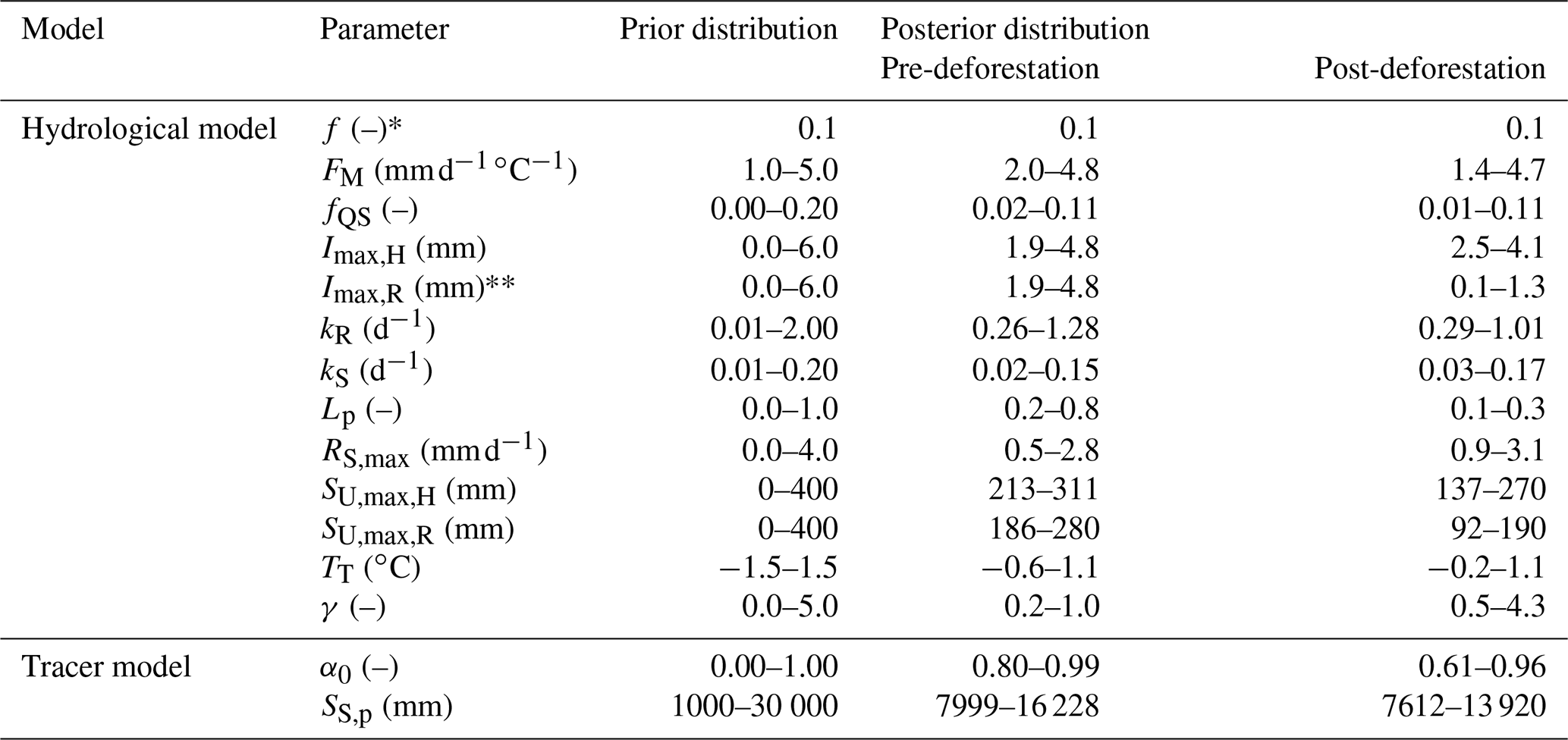
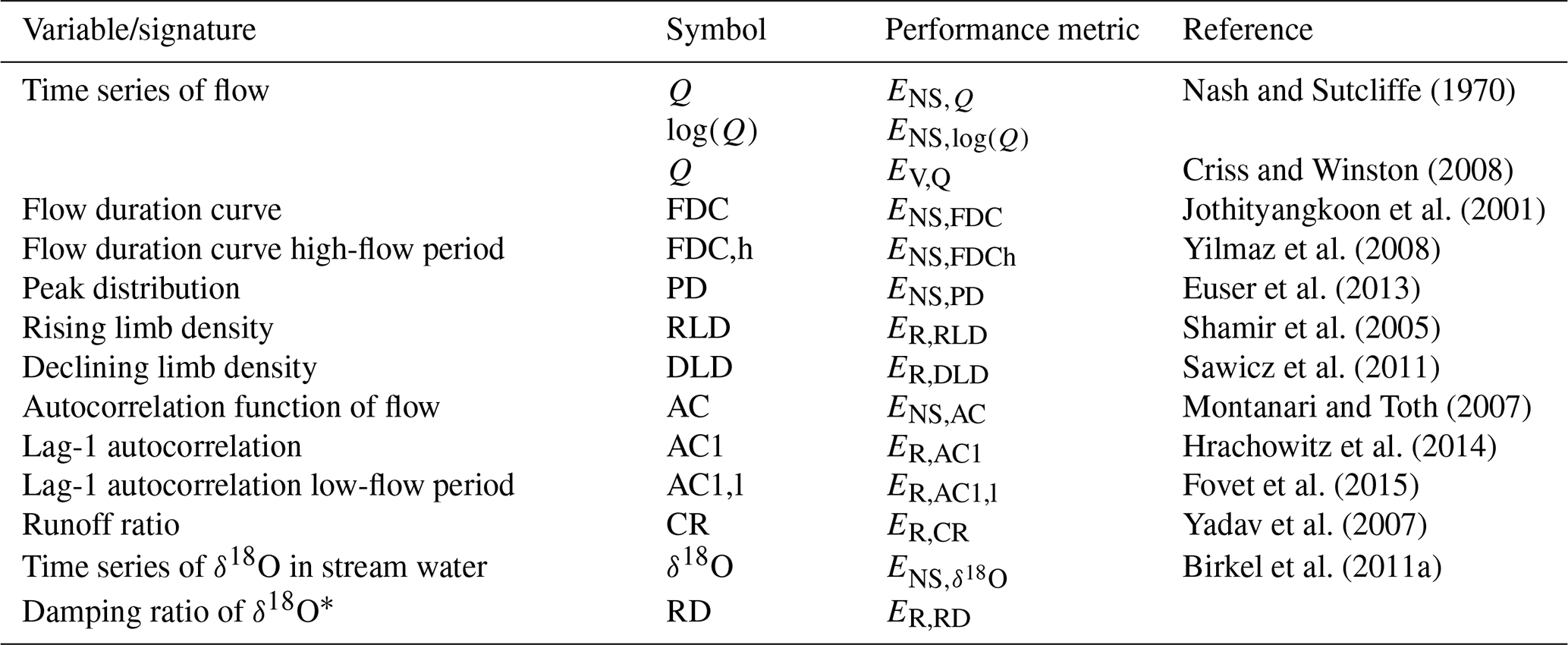
Table 3 Signatures of flow and δ¹⁸O and the associated performance metrics used for model calibration and evaluation. The performance metrics used include the Nash–Sutcliffe efficiency (E_NS), the volume error (E_V) and the relative error (E_R).

^* $\text{RD}=\frac{{\text{SD}}_{\mathrm{Q}}\left({\mathit{\delta }}^{\mathrm{18}}\mathrm{O}\right)}{{\text{SD}}_{\mathrm{P}}\left({\mathit{\delta }}^{\mathrm{18}}\mathrm{O}\right)}$

4.3 Model calibration and post-calibration evaluation

The model was run with a daily time step and has a total of 14 free calibration parameters, which were calibrated for the model to simultaneously reproduce flow and δ¹⁸O dynamics in the stream. The uniform prior parameter distributions (Table 2) were sampled using a Monte Carlo approach with 3×10⁶ realizations. To limit equifinality (Beven, 2006) and to ensure robust posterior parameter distributions for a meaningful process representation (e.g. Kuppel et al., 2018b), an extensive multi-objective calibration strategy was applied. Briefly, this was done using a total of 14 performance metrics that describe the model's skill in reproducing different signatures associated with streamflow (E_Q) and δ¹⁸O dynamics ($E_{{\mathit{\delta }}^{\mathrm{18}}\mathrm{O}}$) as shown in Table 3.

To be accepted as feasible, solutions had to exceed a threshold value of 0.5 for all performance metrics, with the exception of $E_{\text{NS},{\mathit{\delta }}^{\mathrm{18}}\mathrm{O}}$, for which a threshold of 0.2 was used. To further constrain the model, we only accepted solutions that could reproduce the dynamics in observed soil moisture as well as the average observed magnitudes of canopy throughfall. To do so we used a simplified limits-of-acceptability approach (e.g. Coxon et al., 2014) with a rectangular step function so that all solutions that fall within the limits of the step function receive a weight of 1 while all others are assigned a weight of 0 and are thus rejected (Bouaziz et al., 2021). More specifically, we rejected solutions whose modelled normalized relative soil moisture fell outside the acceptable limits, here defined as ±0.15 of the observed relative soil moisture, in more than 75 % of the time steps in the calibration periods. Similarly, we rejected solutions for which the modelled mean ratio $P_{\mathrm{E}}/P$ in the continuously forested part of the catchment was outside ±0.15 of the observed mean ratio $P_{\mathrm{E}}/P=\mathrm{0.71}$. This strategy was chosen instead of directly calibrating the time series of associated model variables S_U (Eq. 20) and P_E (Eq. 18) to explicitly account for commensurability errors between the point scale and the scale of the model application (Bouaziz et al., 2021). Subsequently, the 14 metrics of the solutions retained as feasible were combined into two equally weighted classes, describing streamflow (Q) and tracer (δ¹⁸O) dynamics, respectively. This then allowed us to obtain solutions with balanced overall model performances using the mean Euclidean distance D_E (–) from the “perfect” model (i.e. D_E=1; Hrachowitz et al., 2014; Hulsman et al., 2020):

$$\begin{array}{ll}{\displaystyle }& {\displaystyle }{D}_{\mathrm{E}}=\\ \text{(14)}& {\displaystyle }& {\displaystyle }\mathrm{1}-\sqrt{{\displaystyle \frac{\mathrm{1}}{\mathrm{2}}}\left({\displaystyle \frac{{\sum }_{n=\mathrm{1}}^N{\left(\mathrm{1}-E_{\mathrm{Q},n}\right)}^{\mathrm{2}}}{N}}+{\displaystyle \frac{{\sum }_{m=\mathrm{1}}^M{\left(\mathrm{1}-E_{{\mathit{\delta }}^{\mathrm{18}}\mathrm{O},m}\right)}^{\mathrm{2}}}{M}}\right)},\end{array}$$

where N=12 is the number of different performance metrics describing streamflow and M=2 the number of different performance metrics for δ¹⁸O. To construct the posterior parameter distributions and the corresponding model uncertainty intervals, the retained parameter sets where then weighted according to a likelihood measure $L=D_{\mathrm{E}}^p$ (cf. Freer et al., 1996), where the exponent p was set to a value of 10 to emphasize models with good overall calibration performance.

In a first step, the model was calibrated for the pre-deforestation period 1 October 2009–31 August 2013. Note that due to a lack of regular and weekly δ¹⁸O precipitation data before 1 October 2010, the performance metric $E_{{\mathit{\delta }}^{\mathrm{18}}\mathrm{O}}$ describing the δ¹⁸O dynamics was computed from that date onwards only. The feasible parameter sets were then used to test the model without further calibration in the post-deforestation period. In a second step, the model was re-calibrated for the 1 September 2013–30 September 2016 post-deforestation period and the changes in the resulting model performance and posterior distributions compared to those from the pre-deforestation calibration. The estimation of the effects of deforestation on TTDs is based on model parameter sets obtained from calibration in the pre-deforestation and post-deforestation periods, respectively.

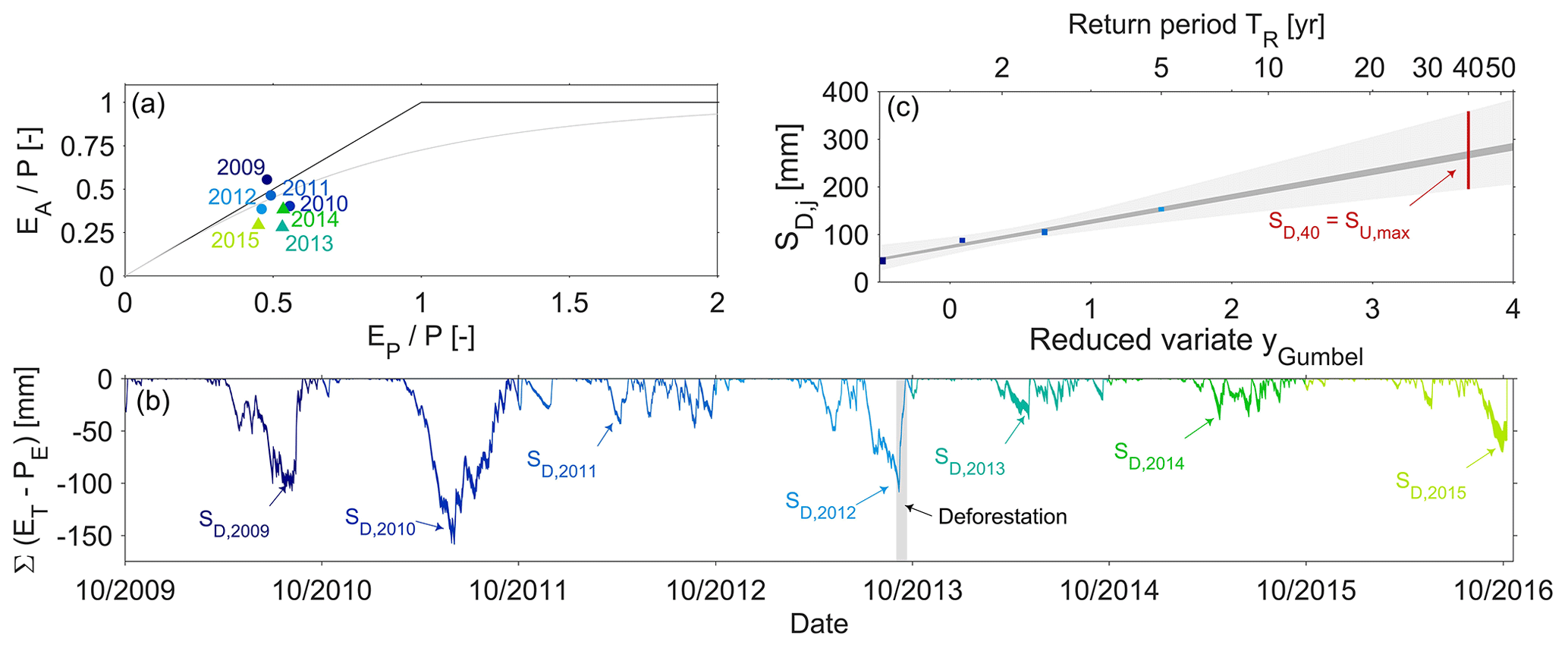
Figure 5 (a) Positions of the individual years of the study period in the Budyko framework. The x axis shows the aridity index $I_{\mathrm{A}}=E_{\mathrm{P}}/P$; the y axis indicates the evaporative ratio $E_{\mathrm{A}}/P$ and the runoff ratio $C_{\mathrm{R}}=\mathrm{1}-E_{\mathrm{A}}/P$. Pre-deforestation years are shown with blueish shades, post-deforestation years with greenish shades. The bold black lines indicate the energy and water limits, respectively. The dashed grey line is the theoretical–analytical Turc–Mezentsev relationship (Turc, 1954; Mezentsev, 1955). (b) The range of time series of storage deficits as computed according to Eq. (2), using values of I_max from 0 to 4 mm. The maximum annual storage deficits S_D,j are indicated by the arrows. The grey shaded area indicates the deforestation period. (c) Estimation of S_U, max as the storage deficit associated with a 40-year return period S_D,40 yr using the Gumbel extreme value distribution for the pre-deforestation period. The blueish dots indicate the range of maximum annual storage deficits S_D,j for each year in the 4-year pre-deforestation period. The dark-grey shaded area indicates the envelope of least-square fits for the individual values of I_max. The light-grey shaded area indicates the envelope of the 5th$/$95th confidence intervals. The red line shows the plausible range for S_U, max.

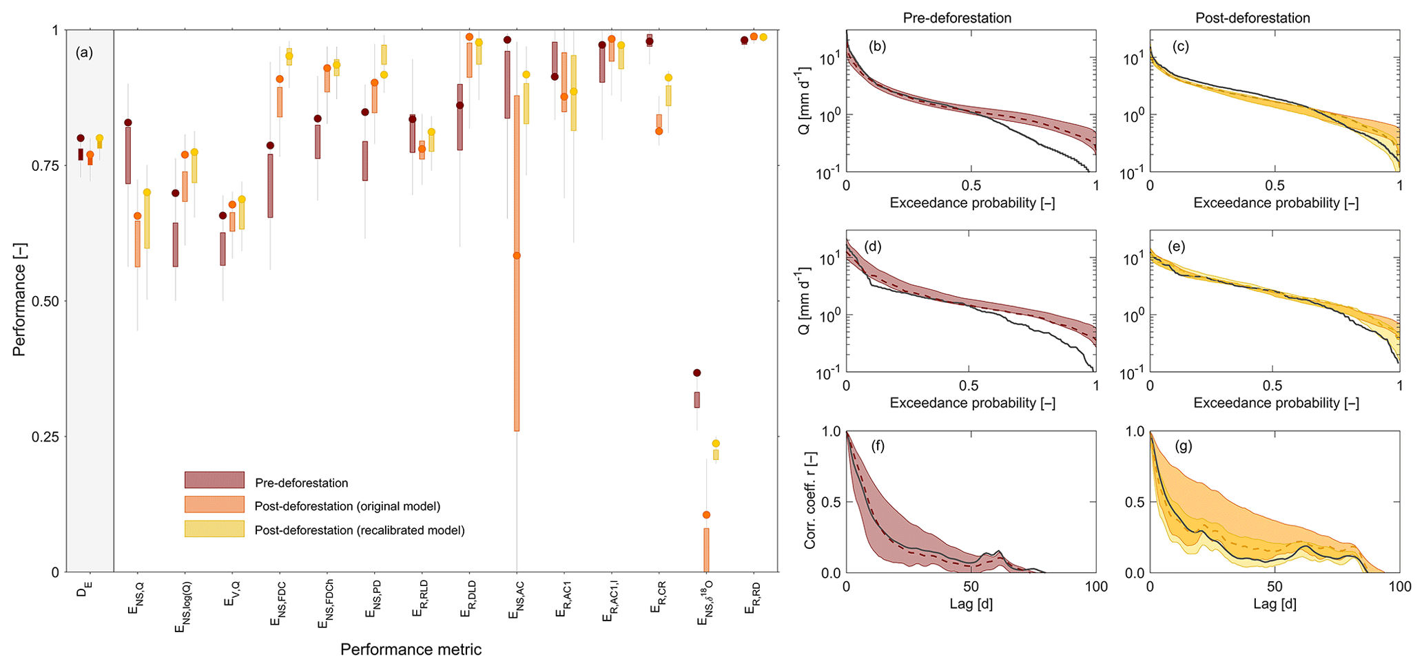
Figure 6 (a) Model performance metrics for all variables and signatures. D_E is the Euclidean distance to the perfect model. It combines all other performance metrics (Table 3) into one number (Eq. 42). All performance metrics are formulated in a way that a value of 1 indicates a perfect fit. The boxplots summarize the performances of all parameter sets retained as feasible. The circle symbols indicate the performance of the best-performing model in terms of D_E. The dark-red shades indicate pre-deforestation model performance based on calibration in the pre-deforestation period. Orange shades indicate post-deforestation performance using the pre-deforestation parameter sets without further re-calibration. Yellow shades show the post-deforestation performance after model re-calibration in the post-deforestation period. (b, c) show flow duration curves, (d, e) show the peak distributions and (f, g) show the autocorrelation functions for the pre- (red) and post-deforestation periods (orange and yellow), respectively. The black lines indicate the observed values, the dashed lines indicate the best fits and the shaded areas indicate the 5th$/$95th uncertainty interval of all solutions retained as feasible. The dark-red shades indicate pre-deforestation model results based on calibration in the pre-deforestation period. Orange shades indicate post-deforestation model results using the pre-deforestation parameter sets without further re-calibration. Yellow shades show the post-deforestation model results after model re-calibration in the post-deforestation period.

5 Results

5.1 Observed deforestation effects on the hydrological system

Initial analysis of water balance data suggests that the hydro-meteorological conditions as expressed by the aridity index $I_{\mathrm{A}}={\stackrel{\mathrm{‾}}{E}}_{\mathrm{P}}/\stackrel{\mathrm{‾}}{P}$ do not show significant differences between the pre-deforestation ($I_{\mathrm{A}}=\mathrm{0.50}\pm \mathrm{0.02}$) and post-deforestation periods ($I_{\mathrm{A}}=\mathrm{0.51}\pm \mathrm{0.03}$), respectively (Fig. 5a). However, and in spite of these comparable climatic conditions, the results show a shift in the partitioning of water fluxes between runoff Q and actual evaporation E_A (note that $E_{\mathrm{A}}=E_{\mathrm{I}}+E_{\mathrm{T}}$). While the fraction of precipitation that was released into the atmosphere as vapour was reduced (${\stackrel{\mathrm{‾}}{E}}_{\mathrm{A}}/\stackrel{\mathrm{‾}}{P}$; Fig. 5a), the mean runoff ratio ($C_{\mathrm{R}}=\mathrm{1}-{\stackrel{\mathrm{‾}}{E}}_{\mathrm{A}}/\stackrel{\mathrm{‾}}{P}$) increased correspondingly from $C_{\mathrm{R}}=\mathrm{0.55}\pm \mathrm{0.04}$ to $C_{\mathrm{R}}=\mathrm{0.68}\pm \mathrm{0.03}$ after deforestation of 21 % of the catchment with p=0.049 based on a Wilcoxon rank sum test. In absolute terms this entails that, notwithstanding rather stable mean annual precipitation $P=\mathrm{1269}\pm \mathrm{24}$ mm yr⁻¹ and potential evaporation $E_{\mathrm{P}}=\mathrm{632}\pm \mathrm{9}$ mm yr⁻¹ over the entire study period, the annual actual evaporation E_A decreased from 576±11 to 401±6 mm yr⁻¹, whereas annual runoff Q increased by ∼25 % from 694±47 to 870±63 mm yr⁻¹.

In spite of similar climatic conditions, the above is reflected in a significantly higher (p=0.047) mean annual maximum storage deficit in the pre-deforestation period than in the post-deforestation period. In the pre-deforestation period values between 105±23 mm for I_max=0 mm and 95±21 mm for I_max=4 mm, respectively, were found (Fig. 5b), whereas in the post-deforestation period the mean storage deficit only reached between 49±10 and 33±7 mm for the same values of I_max (Fig. 5b). Note that in both periods, S_D,j is relatively insensitive to the magnitude of I_max (cf. Gerrits et al., 2009). From the above maximum annual storage deficits S_D,j, the corresponding catchment-scale vegetation-accessible water storage capacity, assuming vegetation adaptation to dry conditions with 40-year return periods (see Sect. 4.1), was estimated at values of $S_{\text{U,\hspace{0.17em}max}}=\mathrm{258}\pm \mathrm{125}$ mm for the pre-deforestation (R²=0.91, p=0.04; Fig. 5c) and $S_{\text{U,\hspace{0.17em}max}}=\mathrm{101}\pm \mathrm{149}$ mm for the post-deforestation period (R²=0.83, p=0.27; not shown).

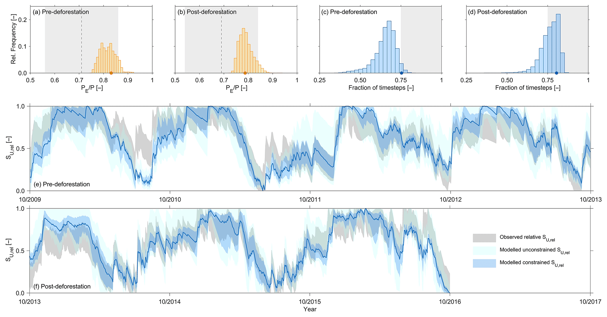
Figure 7 Observed mean $P_{\mathrm{E}}/P$ (dashed line), the range around observed mean $P_{\mathrm{E}}/P$ defined as acceptable (grey shaded area), the distribution of modelled mean $P_{\mathrm{E}}/P$ from all solutions that satisfy the behavioural thresholds for all performance metrics (Table 3) as well as the mean $P_{\mathrm{E}}/$ of the best solution in terms of D_E (orange symbol) for (a) the 2009–2013 pre-deforestation period and (b) the 2013–2016 post-deforestation period. Note that only modelled solutions (yellow) that fall into the acceptable observed range (grey shaded) are kept as feasible. The fractions of time steps in the pre-deforestation (c) and post-deforestation (d) periods in which the modelled relative soil moisture S_U,rel falls within the pre-defined acceptable range around the observed relative catchment-average soil moisture. The blue symbols indicate the best solution in terms of D_E, and the distributions indicate the set of solutions that satisfy the behavioural thresholds for all performance metrics (Table 3). The grey shaded areas indicate the region of acceptable solutions, i.e. solutions that fall at least 75 % of the time steps into the acceptable interval. Note that only modelled solutions (light blue) that fall into the acceptable observed range (grey shaded) are kept as feasible. Pre-deforestation (e) and post-deforestation (f) time series of the acceptable range around the observed normalized, relative soil moisture (light-grey shade) and range of modelled normalized relative soil moisture for all solutions that satisfy all performance metrics (“unconstrained”; light blue) and for the set of feasible solutions that satisfy both $P_{\mathrm{E}}/P$ and soil moisture constraints as shown in (a–d) (“constrained”; blue). The dark-blue line indicates the modelled normalized, relative soil moisture of the best solution in terms of D_E.

Figure 8 Posterior distributions of selected parameters shown as empirical cumulative distribution functions (lines) and the associated relative frequency distributions (bars). Red shades indicate calibration in the pre-deforestation period. Yellow shades indicate post-deforestation calibration. The dots indicate the parameter values associated with the respective best fit models.

5.2 Modelled deforestation effects on the hydrological system

5.2.1 Model calibration for the pre-deforestation period

The model parameter sets retained as feasible after calibration in the 2009–2013 pre-deforestation period reproduce the general features of the hydrograph in that period rather well (Fig. 2c, d), similar to a previous modelling study (Cornelissen et al., 2014). This is true for both the timing and magnitudes of high flows, with an associated Nash–Sutcliffe efficiency E_NS,Q=0.83 for the best-performing model in terms of D_E (Fig. 6a) but also for low flows (E_NS,log(Q)=0.70), with the exception of some overestimation in summer 2011. The modelled runoff ratio comes with C_R=0.54 (5th$/$95th interquantile range (IQR): 0.52–0.58) very close to the observed runoff ratio of C_R=0.55 (E_R,CR=0.98). In addition, the model could also simultaneously mimic most other observed flow signatures reasonably well (Fig. 6a), in particular the flow duration curve (E_NS,FDC=0.79; Fig. 6b), the peak distribution (E_NS,PD=0.85; Fig. 6d) and the autocorrelation function (E_NS,AC=0.98; Fig. 6f). The limits-of-acceptability constraints for $P_{\mathrm{E}}/P$ allowed the identification and removal of a few additional parameter sets (∼5 %) that likely overestimate throughfall P_E (Fig. 7a). The soil moisture constraint was more effective as it allowed us to reject a considerable additional proportion of solutions (>90 %) that did not sufficiently well match the observed soil moisture dynamics according to the pre-defined limits of acceptability (Fig. 7c). With the parameter sets eventually retained as feasible, the modelled temporal dynamics of relative soil moisture broadly reflect the observed ones (Fig. 7e). Similarly, the model captures the substantial attenuation of the precipitation δ¹⁸O variability (E_R,RD=0.98; Fig. 6a) while at the same time largely preserving the limited but visible low-frequency temporal fluctuations in the stream δ¹⁸O composition (Fig. 3a, b). In comparison to the flow performance metrics, the Nash–Sutcliffe efficiency of the δ¹⁸O composition for the best model is somewhat lower ($E_{\text{NS},{\mathit{\delta }}^{\mathrm{18}}\mathrm{O}}=\mathrm{0.37}$; Fig. 6a), which mostly results from the low variability of such a damped signal, where even very small absolute errors (MAE = 0.11 ‰) and a few scattered outliers can lead to very low Nash–Sutcliffe efficiencies (cf. Hrachowitz et al., 2009).

The posterior distributions (Table 2, Fig. 8) show that most model parameters are reasonably well identified. Individually calibrated for their respective landscape class, i.e. hillslope and riparian zone, S_U,max,H=242 mm (5th$/$95th IQR: 213–311 mm) and S_U,max,R=213 mm (186–280 mm) showed similar optimal values and distributions (Fig. 7a, b), reflecting the catchment-wide relatively homogenous forest cover in the pre-deforestation period (Fig. 1). Remarkably, these calibrated values also come close to catchment-scale estimates of $S_{\text{U,\hspace{0.17em}max}}=\mathrm{258}\pm \mathrm{125}$ mm that were directly derived from water balance data without any calibration, as described in Sect. 5.1 (Fig. 5c).

5.2.2 Application of the pre-deforestation model to the post-deforestation period

In a next step, the parameter sets obtained from the above calibration in the pre-deforestation period were used to run the model without further re-calibration in the post-deforestation period. This entails the implicit and clearly wrong assumption that the physical characteristics of the system remained unaffected by deforestation. The consequence of that can be seen in Fig. 2c and d (red line). While the low flows remain well reproduced, the post-deforestation application of the model substantially and systematically underestimates high flows, partly by 50 % or more, such as in November 2013 or August 2014. The inability of the model to reproduce several aspects of post-deforestation high-flow dynamics of the system is also evident in the lower model performance metrics associated with high flows (Fig. 6a). Besides the time series of flow (E_NS,Q=0.65), notably the model's skill in capturing the rising limb density (E_NS,PD=0.78), the autocorrelation function (E_NS,AC=0.58; Fig. 6g) and the runoff ratio (E_R,CR=0.81) were negatively affected. In contrast to the pre-deforestation period, the modelled runoff ratio C_R=0.55 (0.54–0.58) in the post-deforestation period considerably underestimates the observed $C_{\mathrm{R}}=\mathrm{0.68}\pm \mathrm{0.03}$ (Fig. 5a). The problems of describing the high-flow periods are accompanied by the model's reduced ability to describe the post-deforestation δ¹⁸O dynamics in stream water ($E_{\text{NS},{\mathit{\delta }}^{\mathrm{18}}\mathrm{O}}=\mathrm{0.11}$), although the observed general degree of damping of the δ¹⁸O signal (E_R,RD=0.98) remains well reproduced as shown in Figs. 3 and 6a. While the low $E_{\text{NS},{\mathit{\delta }}^{\mathrm{18}}\mathrm{O}}$ values are partly an effect of the above-explained low signal-to-noise ratio of such a damped signal and thus of the chosen performance metric, the model also struggles to adequately reproduce the lower-frequency fluctuations, such as between February and July 2014, when the model indicated rather stable δ¹⁸O values, while the observed values show a slight yet clear increasing trend over the same period (Fig. 3b). Together with the lower overall model performance metric D_E (Fig. 6a), these results illustrate that the pre-deforestation model parameter sets provide an unsuitable characterization of the system characteristics in the post-deforestation period.

5.2.3 Recalibrate the model for the post-deforestation period

To estimate the effect of forest removal on the characteristics of the hydrological system and thus on the model parameters, the model was in a next step recalibrated for the post-deforestation period. This led to a slight improvement of the overall model performance from D_E=0.77 to 0.80 (Fig. 6a). Most notably, it can be observed that the recalibrated model can much better reproduce the increased high flows in that period (Fig. 2c, d), as reflected by improvements in the performance metrics associated with high flows (Fig. 6a), but most notably E_NS,Q=0.70, E_NS,FDC=0.95 (Fig. 6c) or E_NS,AC=0.92 (Fig. 6g). Similarly, the limits-of-acceptability constraints ensured a choice of solutions that broadly reflect the observed throughfall ratios $P_{\mathrm{E}}/P$ (Fig. 7b) as well as the observed soil moisture dynamics (Fig. 7d, f). In addition, and perhaps most importantly, the runoff ratio also increased and was with a modelled value of C_R=0.62 (0.56–0.63) closer to the observed C_R=0.68 (E_R,CR=0.91). This further implies that, in contrast to the initial model, the recalibrated model also features expected reductions of evaporative fluxes E_A by about 10 %, which can be seen in Fig. 2b. Mirroring the improvements in the reproduction of flows, re-calibration also allowed the model to better capture the stream water δ¹⁸O dynamics ($E_{\text{NS},{\mathit{\delta }}^{\mathrm{18}}\mathrm{O}}=\mathrm{0.24}$; MAE = 0.10 ‰; Fig. 6a). While there is little change in the model's ability to mimic the general level of damping of the δ¹⁸O signal (E_R,RD=0.99) and its low-frequency fluctuations, the more pronounced, albeit in absolute terms still small, high-frequency fluctuations as short-term responses to individual storms are better described (Fig. 3a, b).

Inspection of the posterior parameter distributions reveals that the catchment-scale S_U, max experienced considerable reductions after re-calibration. While in the hillslope parts of the catchment, which were less affected by deforestation (∼10 % of the hillslope area; Fig. 1), an average decrease by ∼50 mm to S_U,max,H=212 mm (137–270 mm) can be seen (Fig. 8a), the completely deforested riparian area exhibits an average decrease by ∼100 mm to S_U,max,R=93 mm (92–190 mm; Fig. 8b). As an indicative value, the area-weighted catchment average S_U, max=199 mm of the best-performing parameter set falls into the plausible range of $S_{\text{U,\hspace{0.17em}max}}=\mathrm{101}\pm \mathrm{149}$ mm as described in Sect. 5.1. While there is little evidence for reductions of I_max on the less deforested hillslopes (Fig. 8d), a clear decrease in interception capacities by on average ∼2 mm to I_max,R=1.1 mm (0.1–1.3 mm; Fig. 8e) can be observed in the fully deforested riparian zone.

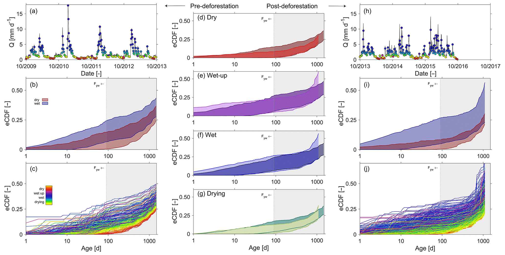
Figure 9 Panels in the left-hand-side column show pre-deforestation (a) discharge, and the coloured dots indicate to which period (dry, wet-up, wet, drying) the individual selected time steps belong; (b) the 5th$/$95th percentiles of the empirical cumulative TTDs for wet (blue) and dry (red) periods, respectively; (c) the ensemble of the individual TTDs at the time steps indicated in (a). Panels in the middle column (d–g) compare the 5th$/$95th percentiles of empirical cumulative TTDs between pre-deforestation (dark shades) and post-deforestation (light shades) periods for dry, wet-up, wet and drying conditions, respectively. Panels in the right-hand-side column show post-deforestation (h) discharge, and the coloured dots indicate to which period (dry, wet-up, wet, drying) the individual selected time steps belong; (i) the 5th$/$95th percentiles of the empirical cumulative TTDs for wet (blue) and dry (red) periods, respectively; (j) the ensemble of the individual TTDs at the time steps indicated in (h). All distributions shown are truncated at 3 (post-deforestation) or 4 years (pre-deforestation), which coincides with the tracked periods. For the remaining fractions, i.e. the difference to 1, it can only be said that they are older than 3 or 4 years but nothing more than that. The grey shaded areas indicate regions with ages >3 months, thereby exceeding F_yw.

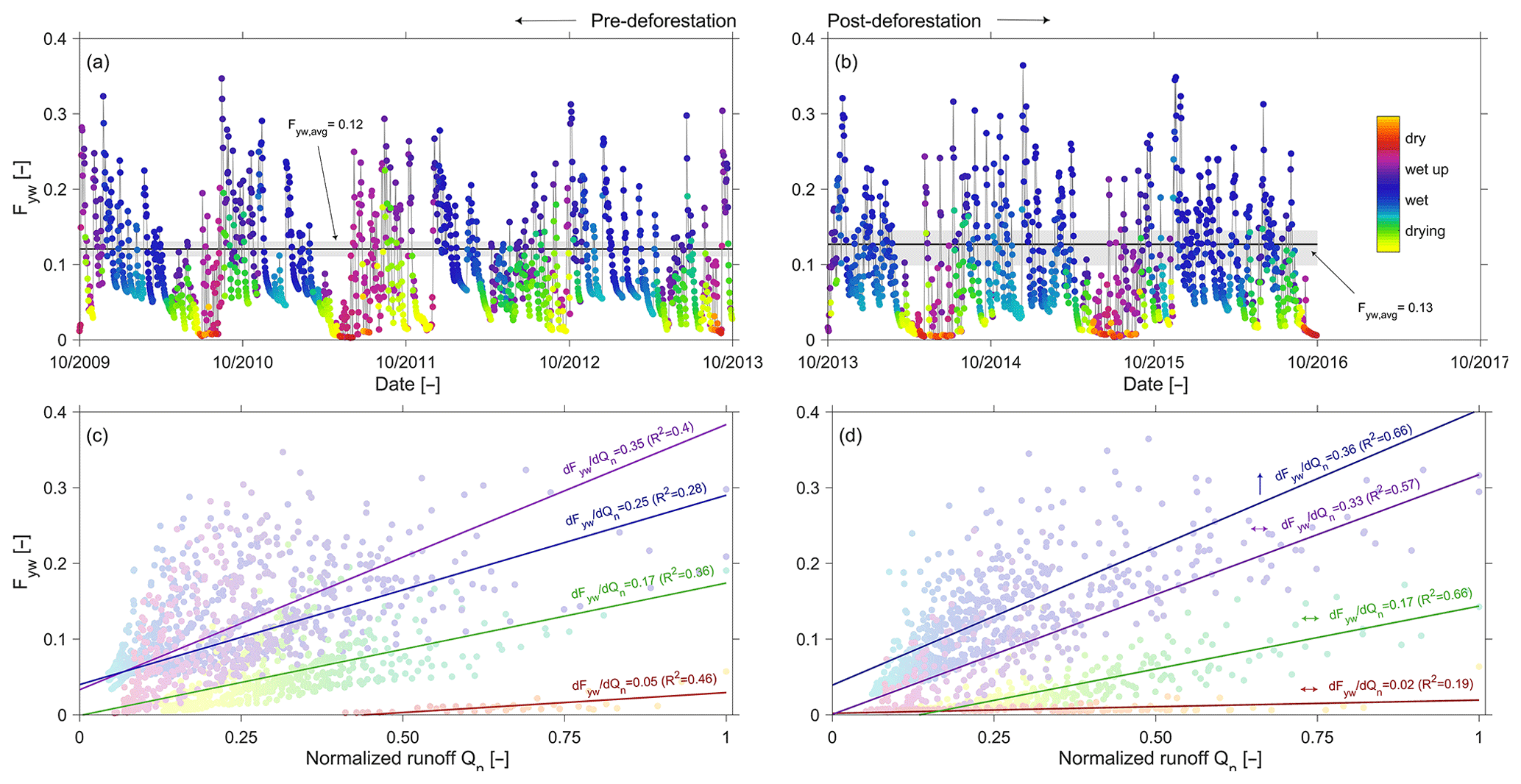
Figure 10 (a, b) Pre- and post-deforestation time series of young water fractions F_yw in discharge. The colour code indicates the transition between dry, wetting-up, wet and drying conditions. The bold black line shows the mean F_yw of the best model fit, and the grey shaded area shows the 5th$/$95th percentile of F_yw for all feasible model solutions; (c, d) pre- and post-deforestation sensitivity of F_yw to discharge, using the same colour code as above to indicate dry, wetting-up, wet and drying conditions. The arrows in (d) indicate whether there are statistically significant (↑; p<0.05) changes or not (↔) in the sensitivities between the post-deforestation period and the pre-deforestation period.

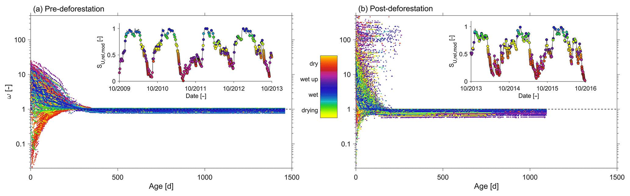
Figure 11 Individual catchment overall SAS ω functions for individual time steps under different wetness conditions in the (a) pre-deforestation period and (b) post-deforestation period. The insets show the relative water content in $S_{\text{U,rel,mod}}=S_{\mathrm{U}}/S_{\text{U,\hspace{0.17em}max}}$ at the individual time steps.

5.3 Deforestation effects on travel time distributions, SAS functions and young water fractions

While the volume-weighted mean δ¹⁸O compositions of observed precipitation with −7.9 ‰ and stream water with −8.2 ‰ are comparable, a substantial difference in their fluctuations, with standard deviations of 3.6 ‰ and 0.2 ‰, respectively, is evident (Fig. 3a, b). This difference suggests a remarkably elevated degree of damping rarely found elsewhere (e.g. Speed et al., 2010), indicative of the importance of old water contributions to the stream in the study catchment. No significant difference in damping ratios was observed between the pre- and post-deforestation periods, which further corroborates the prevalence of old water.

Tracking the δ¹⁸O signals through the model then allowed us to estimate TTDs. Note that any results reported hereafter are necessarily conditional on the assumptions made in and the uncertainties arising from the modelling process.

In general and consistent with the observed high degree of damping, it was found that pre-deforestation of the system was characterized by rather old water. The range of truncated TTDs of stream water exhibits considerable variability in response to changing wetness conditions, with on average about 27 % of the discharge younger than 3 years (Fig. 9b, c). In spite of the low mean F_yw∼0.12 (Fig. 10a), stream water can contain up to 34 % water younger than 3 months (i.e. F_yw∼0.34) for individual storm events in the wet period while frequently dropping to <1 % during elongated summer dry periods (Figs. 8c, 9a), similar to what has been reported elsewhere (e.g. Gallart et al., 2020b). It can also be observed that the age composition of stream water (Fig. 9c) and the associated F_yw (Fig. 10a) do considerably vary throughout wet periods. Dry periods are characterized by considerably less variability and more stable stream water TTDs. This is further corroborated by the significantly higher sensitivity of F_yw to changes in streamflow in wet-up and wet periods ($\mathrm{d}{F}_{\text{yw}}/\mathrm{d}{Q}_{\mathrm{n}}\sim \mathrm{0.35}$ and 0.25, respectively) as compared to dry periods ($\mathrm{d}{F}_{\text{yw}}/\mathrm{d}{Q}_{\mathrm{n}}\sim \mathrm{0.05}$; Fig. 10c). In spite of the low mean F_yw∼0.12 (Fig. 10a), the above also entails that very fast switches towards higher young water fractions can be observed when the system is wetting up after dry periods as well as for storm events throughout the wet season. In general, the above observations are also encapsulated in the catchment-overall storage-age selection functions ω that represent the ratio of stream water TTD over the combined RTD of all model storage elements (Benettin et al., 2015a). While for dry periods undersampling of young water ages with relatively little variability is evident, it can also be seen that in particular during wet-up and wet periods a considerable yet highly variable preference for very young water can be seen (Fig. 11a), similar to what has been reported previously in other environments (e.g. Benettin et al. 2015a; Remondi et al., 2018).

The overall picture did not change in the post-deforestation period. Similarly to the pre-deforestation period, the TTDs can exhibit considerable variability. However, in contrast to the pre-deforestation period, and depending on the wetness conditions, considerable shifts towards younger water can be observed for the TTDs (Fig. 9d–g). There are little discernible changes in F_yw during the dry summer months (Fig. 9d). However, storms in wet-up periods, mostly during autumn, led to considerable increases in the fractions of water younger than 10–20 d (Fig. 9e). During wet periods clear shifts towards younger water can be observed throughout the entire spectrum of tracked ages (Fig. 9f). During the wet period ∼36 % of the stream water is on average younger than the tracked 3 years (Fig. 9i). The mean F_yw only slightly increased to 0.13 (Fig. 10b) compared to 0.12 in the pre-deforestation period (Fig. 10a), which corroborates earlier results by Stockinger et al. (2019) that suggested only minor fluctuations in mean F_yw over multiple moving time windows. For individual winter storm events, F_yw slightly increased to up to ∼0.37 (Figs. 9j, 10b) compared to F_yw of up to ∼0.34 in the pre-deforestation period (Figs. 9c, 10a). Besides the generally higher F_yw during wet periods, the F_yw became more sensitive to flow during wet conditions, with $\mathrm{d}{F}_{\text{yw}}/\mathrm{d}{Q}_{\mathrm{n}}\sim \mathrm{0.36}$ (Fig. 10d), similar to what has been previously reported by von Freyberg et al. (2018) and Gallart et al. (2020a). The above-described post-deforestation changes are also manifest in the corresponding storage-age selection function ω (Fig. 11b) for that period. While the degree of undersampling of young water during dry periods significantly decreased, a substantially higher preference for young water during wet-up and wet periods can be observed than during the pre-deforestation period, with a clear overall shift towards younger water for all wetness conditions.

6 Discussion

6.1 Observed deforestation effects on the hydrological system

The observed post-deforestation changes to the hydrological response, in particular the increase in C_R from ∼0.55 to ∼0.68, correspond well to the findings of an earlier study in the Wüstebach, based on a shorter study period (2011–2015; Wiekenkamp et al., 2016), which estimated an increase in C_R from ∼0.58 to ∼0.66 during that period using eddy-covariance measurements. The overall pattern found here also broadly reflects the effects of land cover/use change in many different environments (Creed et al., 2014; Jaramillo and Destouni, 2014; Renner et al., 2014; van der Velde et al., 2014; Moran-Tejada et al., 2015; Nijzink et al., 2016a; Zhang et al., 2017; Jaramillo et al., 2018). The vast majority of these studies suggest that forest removal leads to an increase in the runoff ratio C_R at the cost of reduced evaporation E_A, although the magnitudes of these changes do substantially vary between individual catchments and studies, which is consistent with our physical understanding of the importance of forest for transpiration in hydrological systems.

Under the assumption that reduction of E_A is largely a direct consequence of forest removal in the Wüstebach, a plausible hypothesis to directly attribute this shift in water partitioning from E_A to Q to a physical process can be formulated as follows: the roots of harvested trees stopped extracting water for transpiration from the sub-surface. In addition, the limited turbulent exchange of vapour at depth effectively limits soil evaporation to the first few centimetres of the soil (e.g. Brutsaert, 2014). Thus, the felling of trees led to a situation where under comparable atmospheric water demand E_P, water volumes held at depths below that and previously within the reach of active roots became largely unavailable for transpiration and evaporation after deforestation. This implies that the water volumes accessible to satisfy atmospheric water demand, i.e. S_U, max and I_max, are drastically reduced. Most notably, the available water balance data suggest that catchment-scale S_U, max decreased from pre-deforestation $S_{\text{U,\hspace{0.17em}max}}=\mathrm{258}\pm \mathrm{125}$ mm to post-deforestation $S_{\text{U,\hspace{0.17em}max}}=\mathrm{101}\pm \mathrm{149}$ mm.

Note, however, that in particular the estimates for the post-deforestation period are characterized by considerable uncertainty and therefore need to be understood as merely indicative, as they are inferred from only 3 years of data and a system that is likely to be far from equilibrium, because the deforested part cannot have adapted yet (e.g. Nijzink et al., 2016a; Teuling and Hoek van Dijke, 2020). These considerable uncertainties are also reflected in the surprisingly low post-deforestation S_U, max.

Notwithstanding these limitations, the above results illustrate that here the reduction of transpiration due to deforestation is likely a direct consequence of the considerable reduction of S_U, max and thus the catchment-scale sub-surface pore volume between field capacity and permanent wilting point that can be actively accessed by vegetation to satisfy the evaporative demand. These post-deforestation decreases in transpiration due to reductions in accessible water volumes S_U, max further lead to reduced soil water storage deficits S_D,j (Eq. 2) in dry seasons, which is consistent with observed post-deforestation increases in soil moisture (Wiekenkamp et al., 2016).

6.2 Modelled deforestation effects on the hydrological system

The model application provided further evidence for the central role of S_U, max as a dominant control on the hydrological response as well as for the direct effects of deforestation on S_U, max. The model calibration in the pre-deforestation period resulted in a set of solutions that could simultaneously reproduce multiple signatures, as expressed by 14 individual performance metrics, while also satisfying two additional limits-of-acceptability constraints. Overall this suggests a rather robust representation of the system.

In a next step, the parameter sets obtained from the calibration in the pre-deforestation period were used to run the model without further re-calibration in the post-deforestation period. This entails the implicit and clearly wrong assumption that the physical characteristics of the system remained unaffected by deforestation. As a consequence, that model exhibited a considerably reduced ability to reproduce the hydrological response in the post-deforestation period, in particular high flows as well as the runoff ratio C_R. The latter implies that the model also overestimates post-deforestation evaporative fluxes E_A. Therefore, it can, without re-calibration, not deal with the observed changes in the partitioning between drainage and evaporative fluxes (Fig. 5a). A likely explanation for the pattern produced by the model is that, in contrast to the real world, no reduction in E_A due to the reduced forest cover is achieved because the model still relies on the catchment-scale vegetation-accessible storage volume S_U, max that characterizes the extent of the catchment-scale active root system before deforestation. This S_U, max falsely provides sufficient water supply to sustain E_A at high levels comparatively close to E_P throughout the year (see red line in Fig. 2b), although, in the parts of the catchment where trees were removed, water stored at depths below a few centimetres is not available for significant evaporation anymore in reality. Such an overestimation of S_U, max implies also that in the model a more pronounced water storage deficit can and does develop throughout dry periods. The model therefore assumes that soils dry out to deeper depths. Consequently, to establish connectivity and to eventually generate flow during and after rainstorms, more water needs to be stored in the model than in the real-world system to overcome this deficit. This water is then in the model held against gravity and thus only available for evaporation but not for drainage, thereby underestimating in particular the magnitude of high flows. Although it is reasonable to assume that groundwater recharge is affected in a similar way, the model can better reproduce low flows. The reason for this is that the draining groundwater body, which sustains summer low flows, is, due to limited recharge during these drier periods, largely disconnected from and thus largely unaffected by sub-surface–vegetation interaction in shallower parts of the sub-surface. In the parts of the catchment where trees were removed, a similar reasoning also holds for the interception capacity I_max and the associated likely overestimation of interception evaporation E_I, yet, due to the smaller magnitude of I_max, to a lesser extent than for S_U, max.

Re-calibration of the model in the post-deforestation period led to a considerably improved representation of the hydrological response and in particular of the high flows as well as the runoff ratio C_R. The latter implies that the modelled partitioning of water fluxes and in particular E_A (see orange line in Fig. 2b) is more consistent with the observed post-deforestation reductions in E_A. In addition, analysis of the modelled fluxes indicates that a higher proportion of flows, mostly during wet-up periods, is rapidly released from the root zones as fluxes R_F,H and R_F,R (Fig. 4; Table 1), representing preferential flows. Such a post-deforestation increase in preferential flow occurrence is supported by observations recently reported by Wiekenkamp et al. (2020).

It is of course unsurprising that re-calibration leads to an improved model performance in the post-deforestation period. Without further analysis, such a mere model fitting exercise allows in the presence of model equifinality only little insight into the underlying processes (Beven, 2006; Kirchner, 2006). To gain more confidence that the improvements in the recalibrated model are at least partly due to the right reasons (Kirchner, 2006), the changes in the posterior parameter distributions resulting from the two calibration runs were thus analysed. In the pre-deforestation period, the range of the posterior distributions of S_U,max,H and S_U,max,R (Fig. 8a, b) as well as the modelled catchment average S_U, max=240 mm, estimated as an area-weighted average of S_U,max,H and S_U,max,R, come close to the catchment-scale estimate of $S_{\text{U,\hspace{0.17em}max}}=\mathrm{258}\pm \mathrm{125}$ mm that was directly derived from water balance data without any calibration (Fig. 5c). The modelled post-deforestation reductions of S_U,max,H and S_U,max,R are evident in the shifts of their respective posterior distributions (Fig. 8a, b) and the lower catchment average S_U, max=199 mm of the best-performing parameter set, falling into the plausible range of $S_{\text{U,\hspace{0.17em}max}}=\mathrm{101}\pm \mathrm{149}$ mm as estimated from water balance data. In addition and quite remarkably, the re-calibrated model is able to broadly represent the differences in forest removal on the hillslopes and in the riparian zone. While in the fully deforested riparian area S_U,max,R decreased by ∼100 mm (Fig. 8b), S_U,max,H on the only partly deforested hillslopes decreased by merely ∼50 mm (Fig. 8a). Similarly, there is little evidence for reductions of I_max,H on the less deforested hillslopes (Fig. 8d). However, a clear decrease in interception capacities by on average ∼2 mm to I_max,R=1.1 mm (0.1–1.3 mm; Fig. 8e) can be observed in the riparian zone. Comparing to the posterior distributions of other parameters, the results illustrate that the storage parameters S_U, max and I_max of the completely deforested riparian zone, and to a lesser extent of the hillslope, were subject to the most pronounced changes. For most other parameters, the pre- and post-deforestation posterior distributions exhibit much less pronounced differences (Fig. 8). Together, these results suggest that deforestation mostly affects S_U, max and I_max, while there is less evidence for systematic changes in other parameters. However, it can also be observed that the individual parameter values associated with the best model solutions in the pre- and post-deforestation periods, respectively, do vary to a stronger degree for most parameters. Notwithstanding the distinct overall effects of forest removal on the individual posterior distributions, this clearly highlights the influence of parameter compensation effects and related uncertainties. This is also illustrated by a few parameters, such as R_S,max (Fig. 8c, Eq. 22), that remain poorly constrained.

It was hypothesized above that reductions in evaporative fluxes are directly and exclusively linked to reduced water volumes S_U, max and I_max, respectively, which are accessible and available for evaporation and transpiration at the catchment scale. In the theoretical ideal case, the representations of the associated storage capacities in the model, i.e. the parameters S_U, max and I_max, should thus be the only ones to significantly change after deforestation. However, note that this is unlikely for two reasons. First, while it is plausible to assume that these storage capacities are significantly affected by forest removal, it is not unlikely that other system characteristics and their mutual interactions, so far unknown and not considered, are similarly influenced, potentially causing considerable ontological uncertainty. Second, model parameter interactions that arise as artefacts to compensate overly simplistic process representations and/or data uncertainty are also likely to affect parameters seemingly unrelated to deforestation. Note that in spite of these uncertainties and the associated compensation effects, in particular S_U, max remains rather well constrained. However, after preliminary unsuccessful testing, no further attempts were made to re-calibrate only the above discussed four storage parameters, i.e. S_U,max,H, S_U,max,R, I_max,H and I_max,R, acknowledging the limitations introduced by parameter compensation effects.

Overall these results suggest that the model formulation together with the multi-objective calibration strategy ensured the identification of solutions that provide a robust description of the system and allow a simultaneous representation of flow and isotope dynamics in the stream. There are indications that at least some processes and parameters can be directly linked to real world quantities. In particular, the results provide strong evidence that the parameters S_U,max,H and S_U,max,R are not merely abstract quantities, but that it is plausible to assume that they, taken together, provide a catchment-scale representation of vegetation-accessible and vegetation-accessed water volumes, which can be estimated based on water balance data without calibration as defined by Eq. (2), thereby providing an alternative to small-scale in situ observations. As such, the parameter S_U, max is also a means to directly and independently estimate the catchment-scale effects of deforestation, and plausibly other types of land cover disturbances, on sub-surface system properties, which underlie and control the changes in the post-disturbance partitioning of water fluxes into drainage and evaporative fluxes.

6.3 Deforestation effects on travel time distributions, SAS functions and young water fractions

Tracking water fluxes through the system, it was observed that wet periods are characterized by substantially more variability and more stable stream water TTDs than dry periods. This is largely a consequence of increased bypass flow that has little interaction with resident water as the system gets wetter and that may reach the stream over preferential flow paths and increased contributions from the riparian zone with its shorter flow paths. In other words, in a wet system where little additional water can be stored, the precipitation volumes of individual storm events control the shape of TTDs, resulting in considerable variability (Heidbüchel et al. 2020). In the summer dry season, however, precipitation is to a higher degree buffered in the root zone and used for transpiration (Stockinger et al., 2014). Conversely, streamflow is then mostly sustained by groundwater which is characterized by large volumes of older water. This effectively attenuates fluctuations by the proportionally much lower volumes of younger precipitation water that cannot be stored and is thus quickly released to the stream.

In particular, at the beginning of the wet period, elsewhere also referred to as “autumn flush” (e.g. Dawson et al., 2011), the switches towards younger water at given flow levels occur considerably faster in the post-deforestation period than in the pre-deforestation period. Therefore, where, at the same discharge, previously relatively little young water reached the stream, a much higher fraction of young water can now be observed in the stream. Underlining the role of transpiration (e.g. Douinot et al., 2019; Kuppel et al., 2020), this is a direct effect of the reduced evaporative removal of relatively young near-surface water (Maxwell et al., 2019) in the post-deforestation period, which in turn is intimately linked to the reduced water supply for evaporative fluxes, i.e. smaller storage volumes S_U, max and I_max. This modelled relatively young, surface-near water, not taken up by vegetation anymore is thus to a higher degree flushed from the system mostly via preferential flow paths to the stream (i.e. R_F,H, R_F,R) and thus bypassing older resident water with little exchange, which is consistent with recent observations of more frequent activation of preferential flow paths (Wiekenkamp et al., 2020). Once connectivity and the associated higher degree of bypass flow are established in the wet period, the post-deforestation peak sensitivity of $\mathrm{d}{F}_{\text{yw}}/\mathrm{d}Q$ to flow increased to ∼0.36, as under these conditions when little additional water can be stored in the shallow sub-surface, F_yw is largely controlled by magnitude of the individual precipitation signals and to a lesser extent by the footprint of the pre-storm history of evaporative fluxes in the shallow sub-surface storage. In contrast, no significant post-deforestation changes could be observed for the sensitivity of F_yw to discharge during dry periods, as during that period, the composition of water ages is controlled by large volumes of old water.

Altogether these results suggest that even in systems dominated by old water, such as the Wüstebach, the removal of forest has the potential to increase the importance of bypass flow through fast flow paths and thus increase the risk of fast, often underestimated propagation of contaminant pulses into groundwater and stream water (e.g. Hartmann et al., 2021).

6.4 Uncertainties, unresolved questions and limitations

As emphasized above, all results are conditional on the assumptions made throughout the modelling process. These assumptions, present in model structure, parameterization and parameters, can lead to uncertainties. However, notwithstanding these potential uncertainties, extensive preliminary model testing together with the use of multiple model calibration and evaluation criteria suggests that there is relatively strong evidence to support the main results in this study: the post-deforestation reduction of evaporative fluxes can, at least partially, be linked to a relatively clear reduction in the catchment-scale storage capacities S_U, max and I_max, which in turn triggered a shift towards younger water ages in the stream, particularly during wet-up and wet conditions.

This is further corroborated when comparing the estimates of S_U, max to estimates of physically plausible upper limits of S_U, max. By definition, S_U, max is physically bound by the depth of the groundwater table. Although fluctuating, the groundwater table in the Wüstebach remains at depths below 1 m for much of the year even in the riparian zone (Bogena et al., 2015) and can be expected to be considerably deeper on the hillslopes. Thus assuming a conservative upper bound of catchment-average depth of the groundwater table at ∼5 m, assuming that the lowest groundwater table at each point in the catchment is at the elevation of the nearest stream, a porosity of the silty clay loam soil of 0.4 (Bogena et al., 2018) and field capacity at a relative porewater content of 0.5 suggests an upper limit of S_U,max,GW∼1000 mm. However, actual roots are very often shallower than these 5 m of the groundwater table. Although sufficient detailed data on root depths are not available in the study catchment, there is no evidence for systematic and widespread roots extending to below 2 m. This is broadly consistent with direct experimental evidence that roots of temperate forests in general (Schenk and Jackson, 2002) and Picea species in particular mostly remain rather shallow (<1 m; e.g. Schmid and Kazda, 2001) and with indirect evidence that Picea species rarely tap groundwater and are thus comparatively shallow (e.g. Evaristo and McDonnell, 2017). As a conservative back-of-the-envelope calculation, assuming thus a maximum plausible catchment-average root depth of 2 m, which comes close to the average observed soil depth reported in Graf et al. (2014), rather suggests a physically plausible upper limit of S_U,max,RD∼400 mm, which is not exceeded by the water balance inferred catchment-scale estimates of $S_{\text{U,\hspace{0.17em}max}}=\mathrm{258}\pm \mathrm{125}$ mm.

Note that the above also suggests the presence of an unsaturated transition zone between the root zone and the groundwater table, i.e. $S_{\text{U,max,TZ}}=S_{\text{U,max,GW}}-S_{\text{U,max,RD}}\sim \mathrm{600}$ mm. In the absence of root water uptake and likely negligible soil evaporation in that zone the water content will remain close to field capacity for much of the year, except for days when a wetting front infiltrates towards the groundwater. This transition zone can therefore be considered as hydrologically largely passive so that at timescales of more than a few days $\mathrm{d}S/\mathrm{d}t\sim \mathrm{0}.$ However, this zone also provides a mixing volume that affects tracer circulation and thus water ages (Hrachowitz et al., 2015). Given its hydrologically passive nature and following the idea of a parsimonious model to limit uncertainty, we here, in a simplification, implicitly added the mixing volume S_U,max,TZ to the passive groundwater mixing volume S_S,p.

For a meaningful interpretation, two specific observations resulting from our analysis warrant special scrutiny. First, model calibration-based estimations of hillslope S_U,max,H (Fig. 7a) suggest post-deforestation median S_U,max,H reductions of ∼25 % as a consequence of clear cutting only ∼10 % of the hillslope part of the catchment (Fig. 1). While this may be surprising at first, it can be plausibly explained by considerable further thinning of the remaining forest on the hillslopes in 2015, 2 years after deforestation, and thus by reduced catchment-scale transpiration demand. However, no detailed and systematic data on the degree of forest thinning are available to meaningfully test this hypothesis.

Second, our results suggest that a passive mixing volume S_S,p of at least ∼8000 mm is necessary for the model to attenuate the amplitudes of the precipitation δ¹⁸O signals to those in the stream water. Although S_S,p is rather well constrained (Fig. 8h), there has in the past been no hydrogeological evidence for the presence of such a surprisingly large groundwater volume nor for its hydrological relevance in the study catchment. Indeed, the authors are not aware of any catchment-scale study that reported similarly high values for S_S,p or functionally equivalent parameters (e.g. Birkel et al., 2011a, b; Hrachowitz et al., 2013, 2015; Benettin et al., 2013, 2015a; Harman, 2015; van der Velde et al., 2015). However, to achieve the degree of damping observed in the stream water, such a volume is necessary if the current understanding of conservative tracer dynamics holds (e.g. Maloszewski and Zuber, 1982; McGuire and McDonnell, 2006). Reflecting our insufficient knowledge of the depth to which exchange with surface water occurs (e.g. Condon et al., 2020), a potential explanation for this observation is that the frequently layered and fractured structure of the Devonian shale bedrock may provide relatively high-permeability pathways for the circulation of and exchange with water at depth. Another, yet, given the current understanding of the Wüstebach (e.g. Graf et al., 2014), less likely hypothesis is the presence of significant lateral groundwater exchange (e.g. Bouaziz et al., 2018; Hulsman et al., 2021b). In other words, the possibility exists that the sub-surface catchment does not match with the surface catchment (Fig. 1) and that older groundwater is imported from “outside” the surface catchment, while an equivalent volume of younger groundwater is exported, maintaining the mass balance. These are hypotheses to be tested in future studies, as the currently available data do not allow a conclusive answer to this question.

7 Conclusions

The small Wüstebach catchment experienced significant deforestation in 2013. Analysing the effects of this deforestation on the hydrology and stable isotope circulation dynamics in the study catchment, our main findings are the following.

Water balance data suggest that deforestation led to a significant increase in streamflow, accompanied by corresponding reductions of evaporative fluxes. This is reflected by an increase in the runoff ratio from C_R=0.55 to 0.68 in the post-deforestation period despite similar climatic conditions, supporting previous results based on eddy-covariance measurements (Wiekenkamp et al., 2016).

Based on water balance data, this reduction of evaporative fluxes, as a consequence of reduced vegetation water uptake, could at least partly be linked to a reduction of the catchment-scale water storage volume in the unsaturated soil that is within the reach of active roots and thus accessible for vegetation transpiration from S_U, max∼258 mm in the pre-deforestation period to S_U, max∼101 mm in the post-deforestation period.

Estimating S_U, max as the calibration parameter of a process-based hydrological model led to similar conclusions. The catchment-average calibrated model parameters representing S_U, max for both the pre-deforestation and post-deforestation periods, respectively, correspond to ∼240 and ∼199 mm broadly, with S_U, max directly estimated from water balance data. Other model parameters, assumed to have a less direct link to vegetation, exhibited much lower levels of systematic change following deforestation.

Using the model to track the age composition of stream water suggested that, in general, water reaching the stream in the pre-deforestation period was rather old, with a mean young water fraction $F_{\text{yw}}\sim \mathrm{0.12}.$ In spite of the overall low F_yw, clear shifts in the shape of travel time distributions towards younger water can be seen under wet conditions, with young water fractions increasing up to $F_{\text{yw}}\sim \mathrm{0.34}.$

Deforestation and the associated reduction of S_U, max led to shifts in travel time distributions towards younger water. Under wet conditions, this resulted in increases in young water fractions to up to F_yw∼0.37 for individual storms. In contrast, dry-period travel time distributions exhibited only minor changes. Overall the mean fraction of young water in the stream increased to $F_{\text{yw}}\sim \mathrm{0.13}.$

Deforestation resulted in a considerable increase in the sensitivity of young water fractions to discharge under wet conditions from $\mathrm{d}{F}_{\text{yw}}/\mathrm{d}Q=\mathrm{0.25}$ to 0.36. This implies faster switches towards younger water and thus faster routing of solutes during and shortly after storm events and thus faster routing of solutes with increasing wetness.

The above results suggest that deforestation has not only the potential to affect the partitioning between drainage and evaporation, and thus the fundamental hydrological response characteristics of catchments, but also catchment-scale tracer circulation dynamics. In particular for wet and wet-up conditions, sometimes also referred to as “autumn flush”, deforestation in the Wüstebach caused higher proportions of younger water to reach the stream, implying faster routing of water and plausibly also solutes through the sub-surface, thereby also increasing the risk of faster propagation of contaminants into stream water and groundwater.

Overall, this study demonstrates that post-deforestation changes in both the hydrological response and travel times can to a large extent be traced back and attributed to changes in S_U, max, a readily quantifiable catchment-scale sub-surface property (and model parameter) representing the maximum water volume that can be stored within the reach of roots. As such, S_U, max and changes therein provide a quantitative, mechanistic hypothesis that can explain why deforestation in the Wüstebach decreased evaporative fluxes, increased streamflow – particularly generated by preferential flows – and reduced travel times. The catchment-scale quantification of S_U, max based on water balance data therefore provides a potentially valuable way towards meaningful and data-based catchment-scale representation of vegetation-accessible water where soil and root observations are not available at sufficient spatial and temporal detail to meaningfully represent their respective natural heterogeneities. In addition, and perhaps more importantly, the method may also hold considerable potential for the formulation of temporally adaptive root-zone parameterizations in catchment-scale hydrological models for more reliable predictions in a changing environment.