The impact of the spatiotemporal structure of rainfall on flood frequency over a small urban watershed: an approach coupling stochastic storm transposition and hydrologic modeling

The role of rainfall space–time structure, as well as its complex interactions with land surface properties, in flood response remains an open research issue. This study contributes to this understanding, specifically for small (<15 km²) urban watersheds. Using a flood frequency analysis framework that combines stochastic storm transposition (SST)-based rainfall scenarios with the physically based distributed Gridded Surface Subsurface Hydrologic Analysis (GSSHA) model, we examine the role of rainfall spatial and temporal variability in flood frequency across drainage basin scales in the highly urbanized Dead Run watershed (14.3 km²), Maryland, USA. The results show the complexities of flood response within several subwatersheds for both short (<50 years) and long (>100 years) rainfall return periods. The impact of impervious area on flood response decreases with increasing rainfall return period. For extreme storms, the maximum discharge is closely linked to the spatial structure of rainfall, especially storm core spatial coverage. The spatial heterogeneity of rainfall increases flood peak magnitudes by 50 % on average at the watershed outlet and its subwatersheds for both small and large return periods. The framework of SST–GSSHA-coupled frequency analysis also highlights the fact that spatially distributed rainfall scenarios are needed in quick-response flood frequency, even for relatively small basin scales.

1 Introduction

Rainfall spatiotemporal structure plays an important role in flood generation in urban watersheds (Saghafian et al., 1995; Smith et al., 2005a; Emmanuel et al., 2012; Nikolopoulos et al., 2014). Spatial heterogeneities in land use and land cover complicate the translation of rainfall spatiotemporal distribution into flood responses (Ogden et al., 2011; Galster et al., 2006; Morin et al., 2006; Ntelekos et al., 2008; ten Veldhuis et al., 2018; Yin et al., 2016), especially for small catchments (Faurès et al., 1995; Smith et al., 2005b; Zhou et al., 2017, 2019; Yang et al., 2020). The influence of rainfall spatial–temporal structure on flood frequency analysis in urban areas remains an open research issue.

Previous studies have demonstrated the sensitivity of hydrological response to rainfall variability in both space and time (Smith et al., 2012; Ochoa-Rodriguez et al., 2015; Rafieeinasab et al., 2015). Following the advent of rainfall measurement using weather radar (Fulton et al., 1998; Krajewski and Smith, 2002), many studies have highlighted the use of high-resolution rainfall data in assessing rainfall variability over a range of spatial and temporal scales (Berne et al., 2004; Gebremichael and Krajewski, 2004; Moreau et al., 2009; Emmanuel et al., 2012) and how their use could improve runoff estimation (Morin et al., 2006; Smith et al., 2007; Schellart et al., 2012; Wright et al., 2014b; Gourley et al., 2017; Rafieeinasab et al., 2015).

There are conflicting findings on the relative importance of rainfall temporal and spatial characteristics. Paschalis et al. (2014), Ochoa-Rodriguez et al. (2015) and Yang et al. (2016) found that “coarsening” temporal resolution has a stronger impact on flood response than coarsening spatial resolution. Adams et al. (2012) found the space–time averaging effects of routing through the catchment notably remove the impact of spatially variable rainfall at a 150 km² catchment scale. Bruni et al. (2015), in contrast, found a higher sensitivity of modeled flow peaks to spatial resolution rather than the temporal resolution. Peleg et al. (2017) showed an increasing contribution of the spatial variability of rainfall to the variability of flow discharge with longer return periods. Cristiano et al. (2018, 2019) found the spatial aggregation of rainfall data can have a strong effect on hydrological responses. Zhu et al. (2018) examined the influence of rainfall variability on flood frequency analysis and addressed the impact of antecedent moisture in flood generation for various basin scales.

Stochastic storm transposition (SST) was developed as a physically based stochastic rainfall generator for rainfall frequency analysis. Previous studies show that SST with relatively short records (10 or more years) of high-resolution radar rainfall fields can produce reasonable rainfall scenarios with realistic spatial–temporal structure, which cannot be provided by conventional design storm methods. In the conventional approach, the idealized assumptions include idealized rainfall temporal structure, uniformed spatial distribution and 1:1 rainfall–flood return period equivalence (see Wright et al., 2013, 2017; Zhou et al., 2019, and references therein). These assumptions ignore the interaction between the spatiotemporal structure of rainfall and flood response, which increases the uncertainty of frequency estimations. Coupled with hydrological models, the SST-based framework can be used for multiscale rainfall frequency analysis and flood frequency analysis that accounts for rainfall variability and surface characteristics (Wright et al., 2014a, 2020; Yu et al., 2019; Perez et al., 2019).

Previous studies have demonstrated that the relationship between rainfall and flood is scale-dependent, varying with rainfall patterns, basin characteristics and runoff generation processes. However, there is still no clear answer on the relative importance of the temporal and spatial features of rainfall in flood responses (Cristiano et al., 2017). Moreover, studies focusing on small (<15 km²) urbanized basins are relatively few (Peleg et al., 2017), and the issues remain poorly understood.

This study contributes to the understanding of the interaction between rainfall variability and flood response over small-scale urbanized watersheds (<15 km²) for a short-duration rainfall and quick hydrologic response setting. We build on the SST-based rainfall study of Zhou et al. (2019) using the physically based hydrological model implementation introduced by Smith et al. (2015) for the Dead Run watershed outside of Baltimore, Maryland, USA. The framework of SST-based rainfall frequency analysis coupled with a hydrological model provides an effective approach for a detailed flood frequency study (Wright et al., 2014a; Yu et al., 2019). Under the framework, we characterize the spatial and temporal features of rainfall events under different return periods and examine their roles in determining flood frequency in small urban watersheds. The following questions will be addressed: (1) how does flood frequency in small urban watersheds vary with space–time rainfall structure and rainfall magnitude? (2) What are the dominant space–time features of rainfall that control flood peak distribution in small urban watersheds? By answering the above questions, the study can improve the understanding of interactions between rainfall and flood processes in small urbanized areas. In addition, some idealized assumptions used in the conventional rainfall–flood frequency analysis will be questioned.

The paper is organized as follows. In Sect. 2, we introduce the study region and describe the SST-based methodology, the Gridded Surface Subsurface Hydrologic Analysis (GSSHA) model and the metrics used to characterize rainfall and flood response. In Sect. 3, we present model validation and analyses of flood frequency distributions and rainfall–flood relationships. A summary and conclusions are presented in Sect. 4.

2 Data and method

2.1 Study region and data

The study focuses on the highly urbanized 14.3 km² Dead Run (DR) watershed located west of Baltimore, Maryland, USA (Fig. 1). DR is a tributary to the Gwynns Falls watershed, which is the principal study catchment of the Baltimore Ecosystem Study (BES; Pickett and Cadenasso, 2006). The basin has an impervious fraction of approximately 52.3 % (Table 1). The watershed has a dense network of six stream gauges, with drainage areas ranging from 1.2 to 14.3 km² (Fig. 1; Table 1). The subwatersheds were developed after the implementation of the Maryland Stormwater Management Act of 1982 (Maryland, 1982), with many detention infrastructures such as small local ponds. The wealth of data for Dead Run provides exceptional resources to examine rainfall and hydrologic response (Beighley and Moglen, 2002; Meierdiercks et al., 2010; Nelson et al., 2006; Smith et al., 2015; Miller et al., 2021). For example, Meierdiercks et al. (2010) analyzed the impact of storm drains and detention basins on a single storm event in DR, while Ogden et al. (2011) used the Gridded Surface Subsurface Hydrologic Analysis (GSSHA) model to analyze the effects of storm drains, impervious area and drainage density on hydrologic response. Smith et al. (2015) created a DR model using GSSHA to examine the effects of storage and runoff generation processes through analyses of a large number of storm events. Miller et al. (2021) examined the role of stormwater management in urban flood response.

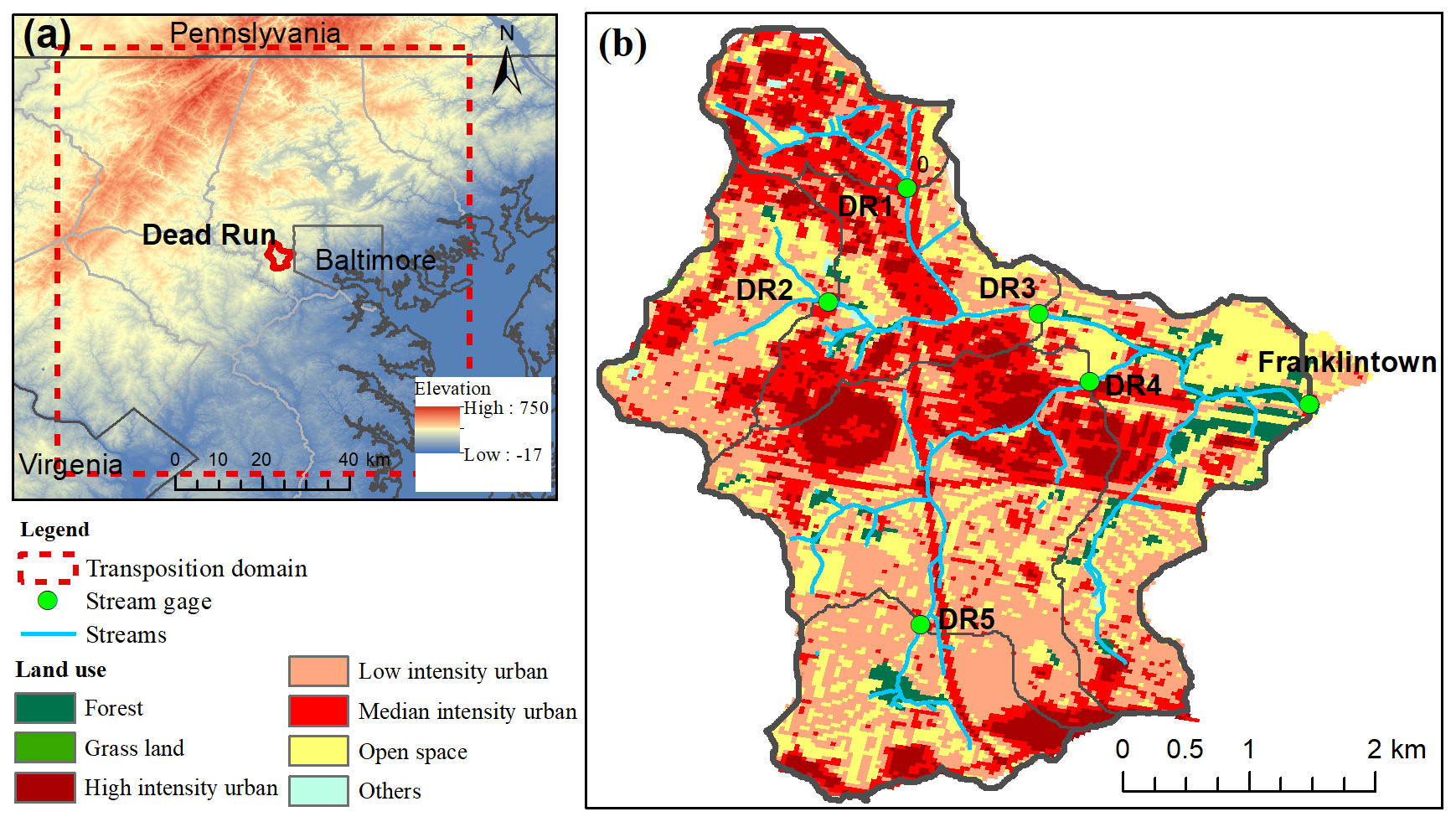
Figure 1 Overview of the Dead Run study region including (a) the location of DR, elevation and transposition domain of SST and (b) land use and land cover and stream gages. The red outline and grey outline in (a) indicate the boundary of the DR watershed and Baltimore City, respectively.

Table 1 Characteristics of the Dead Run watershed (Smith et al., 2015).

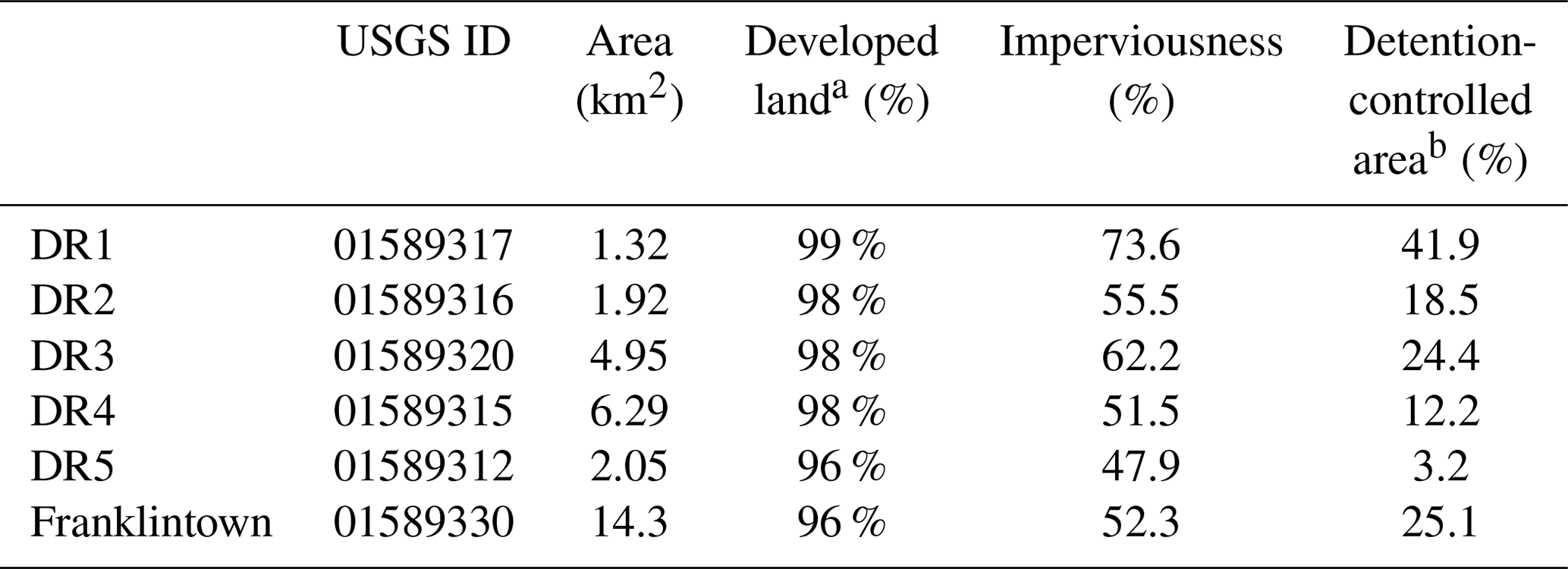
Note: ^a Developed land includes “developed, open space” (>20 % impervious surface), “developed, low intensity” (20 %–49 % impervious surface), “developed, medium intensity” (50 %–79 % impervious surface) and “developed, high intensity” (80 % or more impervious surface). Data source: USGS 2012 National Land Cover Dataset (NLCD). ^b Detention-controlled area refers to the area controlled by detention infrastructure.

High-resolution (15 min temporal resolution, 1 km² spatial resolution) radar rainfall fields for the 2000–2015 period were derived from volume scan reflectivity fields from the Sterling, Virginia WSR-88D (Weather Surveillance Radar-1988 Doppler) radar. The two-dimensional radar rainfall fields are then developed from the reflectivity fields using the Hydro-NEXRAD algorithms (Krajewski et al., 2011) which have been used in rainfall and hydrological studies (Smith et al., 2007, 2012, 2013; Lin et al., 2010; Wright et al., 2014b; Zhou et al., 2017). The Hydro-NEXRAD algorithms include quality control algorithms, Z–R conversion of reflectivity to rainfall rate, time integration and spatial mapping algorithms (Seo et al., 2011). To improve the rainfall estimates, a multiplicative mean field bias correction (Smith and Krajewski, 1991; Wright et al., 2012) is applied on a daily basis using a network of 54 rain gauges in and around the Baltimore County. The bias computation takes the form $B_i=\frac{\sum _{S_i}{G}_{ij}}{\sum _{S_i}{R}_{ij}}$, where G_ij is the rainfall accumulation for gage j on day i, R_ij is the daily rainfall accumulation for the co-located radar pixel accumulation on day i and S_i is the index of the rain gage stations for which both the rain gage and the radar report positive rainfall accumulations for day i. Each 15 min radar rainfall field from day i is then multiplied by B_i. The reader is directed to Zhou et al. (2019) and references therein for further details on the rainfall data and bias correction methods.

Instantaneous discharge data with a resolution of 5 min from the US Geological Survey (USGS) were used for DR-1, DR-2, DR-5 and Franklintown. For DR-3 and DR-4, the discharge data are converted through stage–discharge curves from Lindner and Miller (2012). Streamflow observations for the outlet station at Franklintown extend back to 1960. The subwatersheds have records beginning in 2008.

2.2 GSSHA hydrological model

The distributed physics-based GSSHA model is used to simulate multiscale flood responses. GSSHA is a two-dimensional, distributed-parameter raster-based (i.e. square computational cell-based) hydrologic modeling system. It uses explicit finite difference and finite volume methods in two dimensions on a structured grid to simulate overland flow and in one dimension to simulate channel flow (Downer and Ogden, 2004, 2006). Previous studies of the GSSHA model show that the model with fine grid resolution can produce adequate simulations of flood response, especially when driven by high-resolution radar rainfall fields (Sharif et al., 2010, 2013; Wright et al., 2014a; Cristiano et al., 2019).

In this study, we use the Dead Run model created by Smith et al. (2015). A brief description of the model is provided here; see Smith et al. (2015) for more details. The delineation of the watershed and channel network was based on a 30 m USGS digital elevation model (Gesch et al., 2002). Channel flow overland flow was set with different Manning's roughness coefficients. Additional stream channels were added based on the Baltimore County hydrography geographic information system (GIS) map. Stream cross sections were extracted from a 1 m resolution topography data set for Dead Run developed from lidar. Storm sewers in DR-2 and DR-5 were added using the Baltimore County Stormwater Management GIS map and digitized storm sewer maps. The semicircle's diameter was set to the pipe diameter. Detention basins were represented within the channel with cross sections extracted from the 1 m lidar topographic data.

Several aspects of the model were modified from those used in Smith et al. (2015), primarily to improve computational speed. Infiltration is calculated using Richards' equation (RE) in Smith et al. (2015), while this study uses the three-layer Green–Ampt (GA) scheme. A uniform value of Manning's roughness coefficient of 0.01 is set for all the stream channels for model simplification. Initial soil moisture is approximated to be one-third of the field capacity for each storm event.

2.3 SST procedure

The rainfall scenarios in this study are developed using RainyDay, an open-source SST software package (Wright et al., 2017). The steps used are briefly summarized here; the reader is directed to Zhou et al. (2019) and references therein for further details.

The first step is to identify a geospatial “transposition domain” that contains the watershed of interest. In this study, we use a square 7000 km² transposition domain centered on the DR watershed. Zhou et al. (2019) presented a detailed examination of heterogeneity in extreme rainfall over the transposition domain using a variety of metrics, including storm counts, mean storm depths and intensities, convective activity indicated by lightning observations and analysis of spatial and temporal rainfall structure.

The second step is to identify the largest m storms within the domain at the t h timescale. This collection of storms is referred to as a storm catalog. The storms are selected with respect to the size, shape and orientation of the DR watershed. We henceforth refer to these as “DR-shaped storms.” The m DR-shaped storms are selected from an n-year rainfall record, such that an average of λ=m/n storms per record year is included in the storm catalog. In this study, we chose m=200 storms over the 16-year radar record.

The third step is to randomly sample a subset of k storms from the storm catalog, where k refers to a stochastic number of storms per year. The k is assumed to follow a Poisson-distributed number of storm occurrences with a rate parameter $\mathit{\lambda }=m/n$ storms per year. All rainfall fields associated with a storm are transposed by an east–west distance Δx and a north–south distance Δy, where Δx and Δy are drawn from distributions D_X(x) and D_Y(y), which are bounded by the limits of the transposition domain. Based on the spatial heterogeneity analysis of extreme rainfall in the domain, distributions D_X(x) and D_Y(y) can be set as uniform or nonuniform. In Zhou et al. (2019) and this study, since the assumption of regional homogeneity cannot be relaxed, we used the nonuniform distribution. A two-dimensional probability density function (PDF) of spatial storm occurrence (Wright et al., 2017) is used as the basis for nonuniform spatial transposition (Fig. A1). This step can be understood as generating a “synthetic year” of extreme rainfall events over the domain based on resampling and transposing observations. For each of the k transposed storms, compute the t h basin-average rainfall depth over the watershed. Among the k rainfall depths, the maximum depth is retained as a synthetic t h annual rainfall maximum for the watershed, while the transposed rainfall fields are saved for use as inputs to a GSSHA model simulation.

The fourth step repeats Step 3 S times to recreate multiple years of synthetic t h “annual” rainfall maxima and associated transposed rainfall fields for the watershed. In this study, these steps are repeated S=300 times, and the ordered “annual” maxima are used to generate rainfall return period estimates up to 200 years. A total of 300 such realizations of 200-year series are generated, and the median value of 300 realizations is used to generate estimates for return periods up to 200 years.

2.4 Characteristics of rainfall and hydrologic response

2.4.1 Spatiotemporal characteristics of rainfall

Rainfall statistics were computed for each event, based on radar rainfall data at 15 min, 1 km² resolution, to characterize the spatial and temporal variability of rainfall (following Smith et al., 2002, 2005a; see also Zoccatelli et al., 2011 and Emmanuel et al., 2015). The basin-average rainfall rate (mm h⁻¹) at time t during the storm is given by

$$\begin{array}{}\text{(1)}& M\left(t\right)=\underset{A}{\int }R(t,x)\mathrm{d}x,\end{array}$$

where A is the drainage area (km²), R(t,x) is the rain rate (mm h⁻¹) at radar grid x at time t and T (h) is the time period of the rainfall event. Peak basin-average rainfall rate (mm h⁻¹) is denoted

$$\begin{array}{}\text{(2)}& M_{\max }=\max \mathit{\left\{}M\right(t);t\in [\mathrm{0},T\left]\mathit{\right\}},\end{array}$$

and the storm total rainfall depth (mm) is

$$\begin{array}{}\text{(3)}& R_{\mathrm{sum}}=\sum _{\mathrm{0}}^{T}M\left(t\right).\end{array}$$

To characterize the spatial properties of rainfall, several dimensionless quantities are computed. Fractional coverage of storm core at t is given by

$$\begin{array}{}\text{(4)}& Z\left(t\right)={\displaystyle \frac{\mathrm{1}}{A}}\underset{A}{\int }{I}_{\left(R\right(t,x\left)\right)}\mathrm{d}x,\end{array}$$

where I_(R(t,x)) is the indicator function and equals 1 when $R(t,x)>\mathrm{25}$ mm h⁻¹ or 0 otherwise.

Rainfall location is given by

$$\begin{array}{}\text{(5)}& L\left(t\right)=\underset{A}{\int }\mathit{\omega }(t,x)d\left(x\right)\mathrm{d}x,\end{array}$$

where $\mathit{\omega }(t,x)=\frac{R(t,x)}{\underset{A}{\int }R(t,x)\mathrm{d}x}$, d(x) is the linear distance from point x to the outlet. The rainfall-weighted flow distance is

$$\begin{array}{}\text{(6)}& \mathrm{RWD}\left(t\right)=\underset{A}{\int }\mathit{\omega }(t,x)d_{\mathrm{f}}\left(x\right)\mathrm{d}x,\end{array}$$

where distance function d_f(x) is the flow distance between point x and the outlet. It is calculated as the sum of the overland flow distance from x to the nearest channel and the distance along the channel to the basin outlet. The flow distance d_f(x) is normalized by the maximum flow distance, ranging from 0 to 1. RWD with values close to 0 indicates that rainfall is distributed near the basin outlet, with values close to 1 indicating rainfall concentrated at the far periphery of the basin.

For a uniformly distributed rainfall, the mean RWD is

$$\begin{array}{}\text{(7)}& \stackrel{\mathrm{‾}}{\mathrm{RWD}}=\underset{A}{\int }{d}_{\mathrm{f}}\left(x\right)\mathrm{d}x.\end{array}$$

The dispersion of RWD is

$$\begin{array}{}\text{(8)}& S\left(t\right)={\displaystyle \frac{\mathrm{1}}{\stackrel{\mathrm{‾}}{s}}}\underset{A}{\int }\mathit{\omega }(t,x){\left[d_{\mathrm{f}}\left(x\right)-\stackrel{\mathrm{‾}}{d}\right]}^{\mathrm{2}}\mathrm{d}x,\end{array}$$

where $\stackrel{\mathrm{‾}}{s}=\underset{A}{\int }\left[d_{\mathrm{f}}\right(x)-\stackrel{\mathrm{‾}}{d}{]}^{\mathrm{2}}\mathrm{d}x$, and S is a spatial indicator. S with values < 1 indicates that rainfall is a unimodal distribution, that is, spatially one peak over the watershed, and S with values > 1 indicates that rainfall is a multimodal distribution.

Equations (1)–(3) are typical rainfall characteristics used in conventional rainfall–flood analysis since they reflect the general information of rainfall. Since the basin-averaged index will ignore the potential spatial heterogeneity over the watershed, Eqs. (4)–(8) describe the spatial distribution of rainfall within the area.

2.4.2 Spatiotemporal characteristics of hydrologic response

Flood peak (Q_peak, mm³ s⁻¹), total runoff (Q_sum, mm) and lag time (T_lag, min) are defined as

$$\begin{array}{}\text{(9)}& {\displaystyle }& {\displaystyle }{Q}_{\mathrm{peak}}=\max \left\{Q\left(t\right);t\in T_{\mathrm{d}}\right\}\text{(10)}& {\displaystyle }& {\displaystyle }{Q}_{\mathrm{sum}}=\sum _{\mathrm{0}}^{T_{\mathrm{d}}}Q\left(t\right)\text{(11)}& {\displaystyle }& {\displaystyle }{T}_{\mathrm{lag}}=T_{\mathrm{Fpeak}}-T_{\mathrm{Rpeak}},\end{array}$$

respectively, where Q(t) is the flow discharge at time t, and T_d is the duration of hydrological response, which is from the start of rainfall event to the time when $f\left(t\right)<\mathrm{0.05}\cdot Q_{\mathrm{peak}}$.

3 Results and discussion

3.1 Model validation

We validated the Dead Run GSSHA model through analyses of the 21 largest warm season (April–September) flood events, with peak discharges ranging from 70.3 to 253 m³ s⁻¹ in the 2008–2012 period. The simulated discharge was compared to USGS streamflow observations for all six gaging stations. We assessed peak discharge, peak time and Nash–Sutcliffe efficiency (NSE) (Nash and Sutcliffe, 1970) to examine the performance of the model.

Peak discharge difference is calculated as the difference between the modeled peak and measured peak as a percentage of the measured peak (Fig. 2a). The peak discharge is underestimated at DR2, DR4, DR5 and Franklintown. The median peak discharge difference at the downstream Franklintown gage was −14 %. For the subwatersheds, the modeled peak at DR2 matches observations best, with a median difference of −7.8 %. This represents relatively good performance in reproducing peak discharges for such a large collection of flood events, with various peak discharges ranging from 70 to 253 m³ s⁻¹. The peaks at DR1 are overestimated substantially by 57 % on average. The issue at DR1 was shown before in Smith et al. (2015), who speculate that the watershed contains a large land area that is not represented fully on county storm sewer maps.

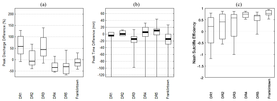
Figure 2 Comparison of (a) flood peak discharges, (b) response times and (c) NSE for 21 historical rainfall events.

The peak time difference is calculated as the time difference between the simulated peak time and measured peak time (Fig. 2b). The median difference ranges from −15 to +10 min, which is within the temporal resolution of the data (15 min for rainfall, 5 min for streamflow). It should be noted that there are several large peak time differences that occurred within the 21 storm events. These are due to the storms that produce multiple discharge peaks. The measured discharge may have the first peak as the largest, while the modeled discharge has the next peak as the largest which is hundreds of minutes later. Nonetheless, the figure shows that the timing of the peak flow is well captured by the model.

The median Nash–Sutcliffe efficiency (NSE) for the 21 events at Franklintown is 0.77 (Fig. 2c). The best NSE at Franklintown is 0.97, indicating that the match between the model and measured data was nearly exact. For the subwatersheds, the best median NSE is at DR-4 with a value of 0.74, while the least median NSE is at DR-1 with a value of 0.21. The results show that the main tendency of flood response is captured by the model.

The hydrograph of the 14 August 2011 storm event is shown as a representative of flood simulations for the 21 events (Fig. 3). The peak discharge difference is −12 % at Franklintown with an NSE of 0.93. Modeled hydrographs match the measured data well at the outlet of the watershed. For the subwatersheds, the peak discharge difference ranges from −38 % at DR4 to 12 % at DR-1. The shape and timing of the modeled response are similar to the measured hydrograph. But the peak discharge is underestimated by more than 30 % at DR-4.

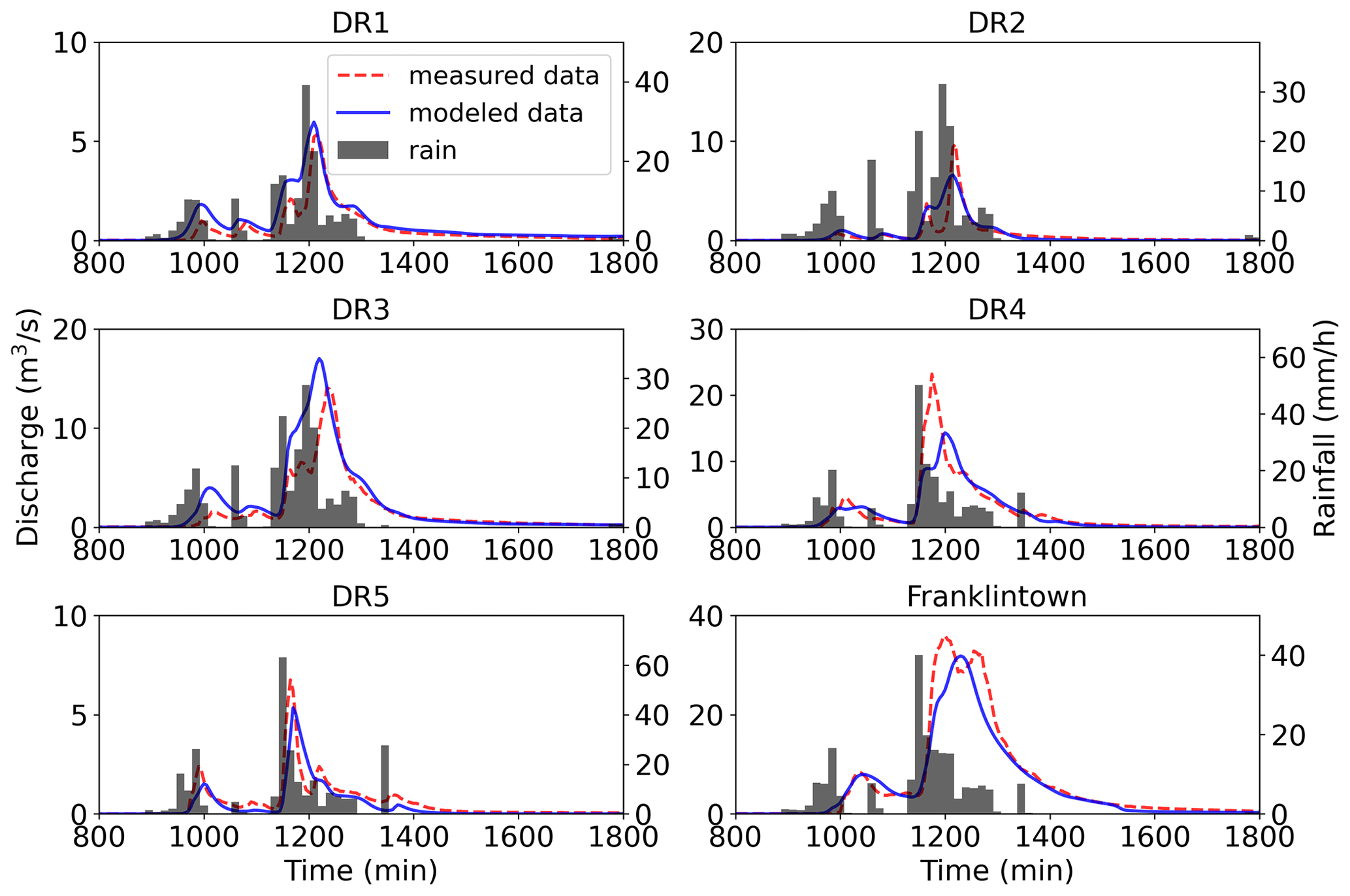
Figure 3 Hydrographs and rainfall for the 14 August 2011 storm event. Time refers to minutes from the start of the model simulation.

It should be noted that the error in simulated response may be attributable to measurement errors tied to stage–discharge curves and conversions of radar reflectivity to rainfall rate, as well as to the features that were simplified within the model, such as initial soil moisture and some aspects of the storm drain network (Smith et al., 2015). For example, it has been documented that the average error of discharge between USGS direct measurements and stage–discharge curves for Franklintown is 17.4 % between 2008 and 2010 (Lindner and Miller, 2012); this error likely grows for high flow conditions. Furthermore, for the rainfall data set used in this study, the median difference of the storm total rainfall between a rain gage and the bias-corrected radar rainfall data for all the pixel of gages over the 21 storms is 22.6 % (Smith et al., 2015). It may also increase the error in the measurements and modeling results.

Overall, the validation shows that the hydrological model can capture the main shape and timing of the measured response in Dead Run. We conclude, therefore, that the model is suitable for the subsequent flood frequency analysis.

3.2 Flood frequency distribution

Under the SST framework, 3 h rainfall scenarios for 10-, 50-, 100- and 200-year return periods were generated (Fig. A2). For each rainfall return period, 300 realizations of rainfall events are used as input to drive the hydrological model. Henceforth, for each rainfall return period, 300 flood responses can be simulated for Franklintown and the five DR subwatersheds.

3.2.1 Flow discharge estimates

The distribution of maximum discharge at the Franklintown gage for rainfall return periods ranging from 10 to 200 years is illustrated in Fig. 4a. To compare the distributions of rainfall and flood peaks, the values are normalized to range from 0 to 1. The normalization is the ratio of values minus the minimum to the maximum minus minimum. The most striking feature is that the distributions of total rainfall and flood peaks are highly variable across the four return periods. The kernel density distribution of rainfall shows a peak at the position of 50th quantile for four return periods. The distribution of flood peaks is more complex. For the 100-year rainfall return period, the kernel density distribution of flood peaks shows a multimodal trend with two small peaks around the 25th and 75th quantiles, which contrasts with the unimodal distribution of rainfall. The following results will show that the flood peak is highly related to spatial rainfall features, implying that the multimodal distribution of flood peaks is associated with the spatial distribution of rainfall. The pronounced difference in the distributions of total rainfall and flood peaks highlights the complex relationship between rainfall properties and flood response in this relatively small urbanized watershed.

Figure 4 Violin plots of (a) normalized flood peak and normalized total rainfall and (b) response time from 10- to 200-year rainfall return periods. (The red dot indicates the mean value. The dashed line in the middle indicates the median value. Upper and lower dashed lines indicate the 75th and 25th quantiles, respectively.) The rainfall return periods are calculated with respect to the average rainfall rate over the entire DR watershed.

The flood response time is calculated as the difference between the time of maximum rainfall rate and maximum discharge (Fig. 4b). Median values of response time are similar under all return periods, ranging from 70 to 83 min, which, given the temporal resolution of rainfall is 15 min, can be similar for all four return periods. It can be concluded that although the flood peak magnitude increases with rainfall return period, the response time is consistent for various rainfall scenarios. This implies in this small highly urbanized watershed the response time is more linked to the drainage system rather than to rainfall characteristics.

Figure 5 demonstrates the simulated hydrographs for the four return periods. The upper and lower spread (75th and 25th quantiles) of the hydrograph indicate the range of variability of simulated hydrographs. For the 10-year return period, the hydrograph is relatively smooth, with a smaller spread. With increasing return periods, the hydrograph is peakier, with a shorter duration of high magnitude discharge. The hydrograph for the 50-year return period shows a transitional shape between small (10-year) and large (100- and 200-year) rainfall return periods. For the 100-year return period, the upper spread shows a tendency toward dual peaks, which cannot be revealed from conventional design flood practices. Since in the conventional rainfall flood frequency approach, the design storm is temporally idealized as a unimodal peak process, using these design storms, the flood response is generally simulated as a unimodal peak process. The above results imply the uncertainty and insufficiency of flood frequency analysis using the conventional methods. For the 200-year return period, the hydrograph is peakiest with a large upper spread.

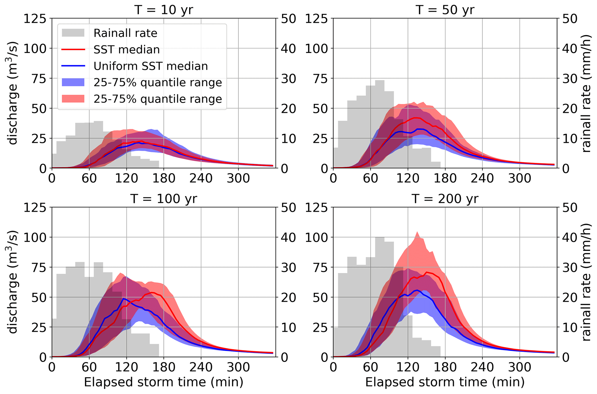
Figure 5 Time series of simulated hydrographs for Franklintown based on the 3 h design storms from 10- to 200-year return periods with spatially uniform (blue) and spatially distributed (red) rainfall. The grey bar indicates the median value of the basin-averaged rainfall rate.

3.2.2 Spatial distribution of flood magnitude

The distribution of flood peaks over the five subwatersheds exhibits contrasting variation with rainfall return periods ranging from 10 to 200 years (Fig. 6). Generally, the basin scale plays an important role in determining the distribution of flood magnitudes. Under the 10-year rainfall return period, DR1 and DR2, with similar basin scales of 1.32 and 1.92 km² respectively, have higher flood peaks and interquartile ranges than other subwatersheds. DR5 (2.05 km²) has comparable flood magnitude with DR4 (6.3 km²) and Franklintown (14.3 km²), while it has a larger interquartile range than the latter two. DR3, with a basin scale of 4.95 km², has comparable flood magnitudes with DR1 and DR2. Under the 200-year rainfall return period, DR2 and DR3 have a slightly larger flood magnitude than DR1. DR5 has the largest interquartile range than others, though its flood peaks are smaller than other small watersheds.

Figure 6 Box plots of normalized flood peaks for Franklintown and five subwatersheds.

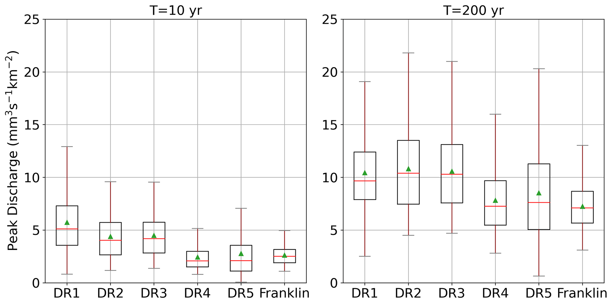
Results show that sub-basin flood distributions vary significantly with rainfall return periods. DR1, with a 33 % larger impervious area and more than double the stormwater-detention-controlled area than DR2 (Table 1), has a 26 % larger median flood peak under a small rainfall return period. For large return periods, DR2 has a slightly larger median peak and a larger peak and interquartile range than DR1. The contrasting peaks in DR1 and DR2 imply that flood peaks are less impacted by impervious areas for extreme storms, while for small rainfall events, detention infrastructure may play less of a role in the detention of flood peaks. DR5, with the smallest detention-controlled area, has the smallest flood peaks under a small rainfall return period. Under a large return period, however, it has the largest changes in peak discharges, with comparable flood peaks with subwatersheds larger than 6 km². DR3 and DR4, with a basin scale of 4.95 and 6.29 km², have contrasting flood magnitude under small and large return periods. DR3, with a larger impervious area and detention-controlled area, has larger flood peaks than DR4. The difference is more significant for small rainfall events, with the median value of flood peak for DR3 more than double that of DR4. From these results, it implies that the impervious area and detention-controlled area play a significant role in determining the peak discharges, but the impact reduces with increasing rainfall return period. The detention infrastructure impacts flood peak and its variability. It should be noted that difficulties remain in attributing specific changes in urban flood peak distributions to specific urbanization characteristics (Zhou et al., 2017). The role of specific urban features in flood responses is beyond the scope of this paper (see Miller et al., 2021, for additional discussion based on analyses of Dead Run discharge observations).

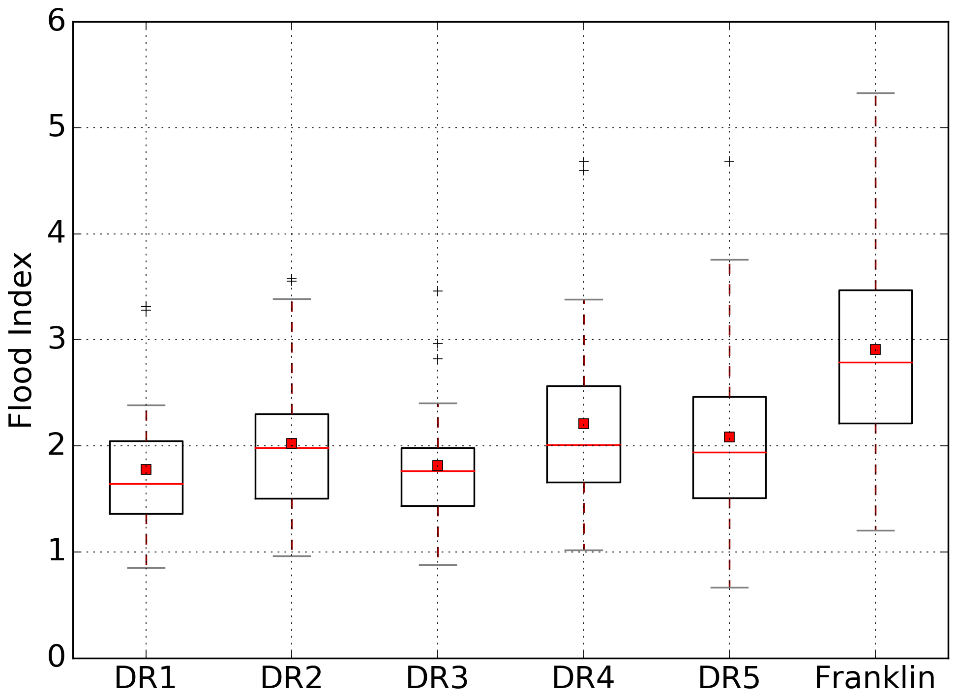
We further examine the spatial distribution of flood magnitude over the Dead Run watershed under the 100-year return period of flood at Franklintown (Fig. 7). The dimensionless flood index is used to compare flood peak magnitudes over the watershed (Lu et al., 2017). The flood index is computed as the maximum flow discharge divided by the computed 10-year flood (Q_10-yr) at the same location, which is set as the median value of 10-year peak discharge at the watershed outlet for each 100-year design storm simulation. At Franklintown, the flood index and its interquartile range are largest across the watersheds, with the median value greater than 2.5. The flood index in the five subwatersheds is relatively lower, within a median value between 1.5 and 2. DR2, as a subwatershed of DR3, has a larger median value than DR1 and DR3. The flood indices at DR1 and DR3 have similar median values and interquartile ranges. Values in DR4 are higher than its subwatershed, DR5, with a median value of 2. The variability of flood magnitudes, indicated by the coefficient of variation (CV), is stable among the watersheds, ranging from 0.30 to 0.39. The spatial distribution of flood magnitude points to the significant heterogeneity of flood distributions over the 14.3 km² watershed. For storm events that produce the same peak discharge return period at the watershed outlet, the subsequent upstream flood response can vary substantially in the Dead Run watershed.

Figure 7 Box plot of flood index across the DR subwatersheds for the 100-year design storms.

3.3 Rainfall–flood relationships

3.3.1 Rainfall structure and flood response

We investigate the relationship between the spatial and temporal characteristics of rainfall and flood response for small and large rainfall return periods based on Spearman's rank correlation (Fig. A3). The peak rainfall rate (M_max), total rainfall (R_sum), fractional coverage (Z), rainfall location (L), rainfall-weighted flow distance (RWD) and the dispersion of RWD (S) are used to characterize rainfall space–time structure. For the 10-year return period, the flood peak is slightly correlated with total rainfall, peak rainfall rate and storm core coverage, with a correlation coefficient of 0.16. For the 200-year return period, in contrast, there is no significant correlation between these features, with correlation coefficients of −0.09, 0.07 and −0.02, respectively, implying a complex and nonlinear relationship between extreme storms and floods in the watershed.

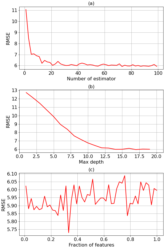
We used random forest regression models to examine the importance of rainfall characteristics to the flood response. Random forests (RF) is an ensemble learning method (Breiman, 2001) that aggregates results from multiple models to achieve better accuracy. RF is one of the most widely used methods for regression and classification. Moreover, it is relatively easy to train and test. In this study, rainfall space–time structure characteristics are used as RF model features. The flood peak is set as the model target. The relationship between rainfall structure and flood peak is then explored under the RF-based regression method. The main parameters of the RF model are tuned by a grid search approach (Probst et al., 2019). The prediction performance is assessed using mean absolute error (MAE), root mean square error (RMSE) and explained variance regression score (E score) (Achen, 2017). Smaller values of MAE and RMSE indicate better model performance. E score ranges from 0 to 1, and a larger value indicates a better model (the training process of the RF model is shown in Fig. A4).

The difference in feature importance is compared between the 10- and 200-year return periods (Fig. 8). For the 10-year return period, peak rainfall rate (M_max) and total rainfall (R_sum) are the most two important features, with a feature importance of 0.17. For the 200-year return period, however, the dispersion of RWD (S) and fractional coverage of storm core (Z) are more important than M_max and R_sum. The rainfall location (L) has the smallest importance for both return periods. The results demonstrate the different relationships between rainfall structure and flood response under small and extreme rainfall events. For extreme storms, the maximum discharge is more closely linked to the spatial structure of rainfall, which is consistent with the results in Peleg et al. (2017) and Zhu et al. (2018). Though it appears that the difference is moderate, for such a small watershed, the tendency of the change of the spatiotemporal rainfall feature importance is noteworthy.

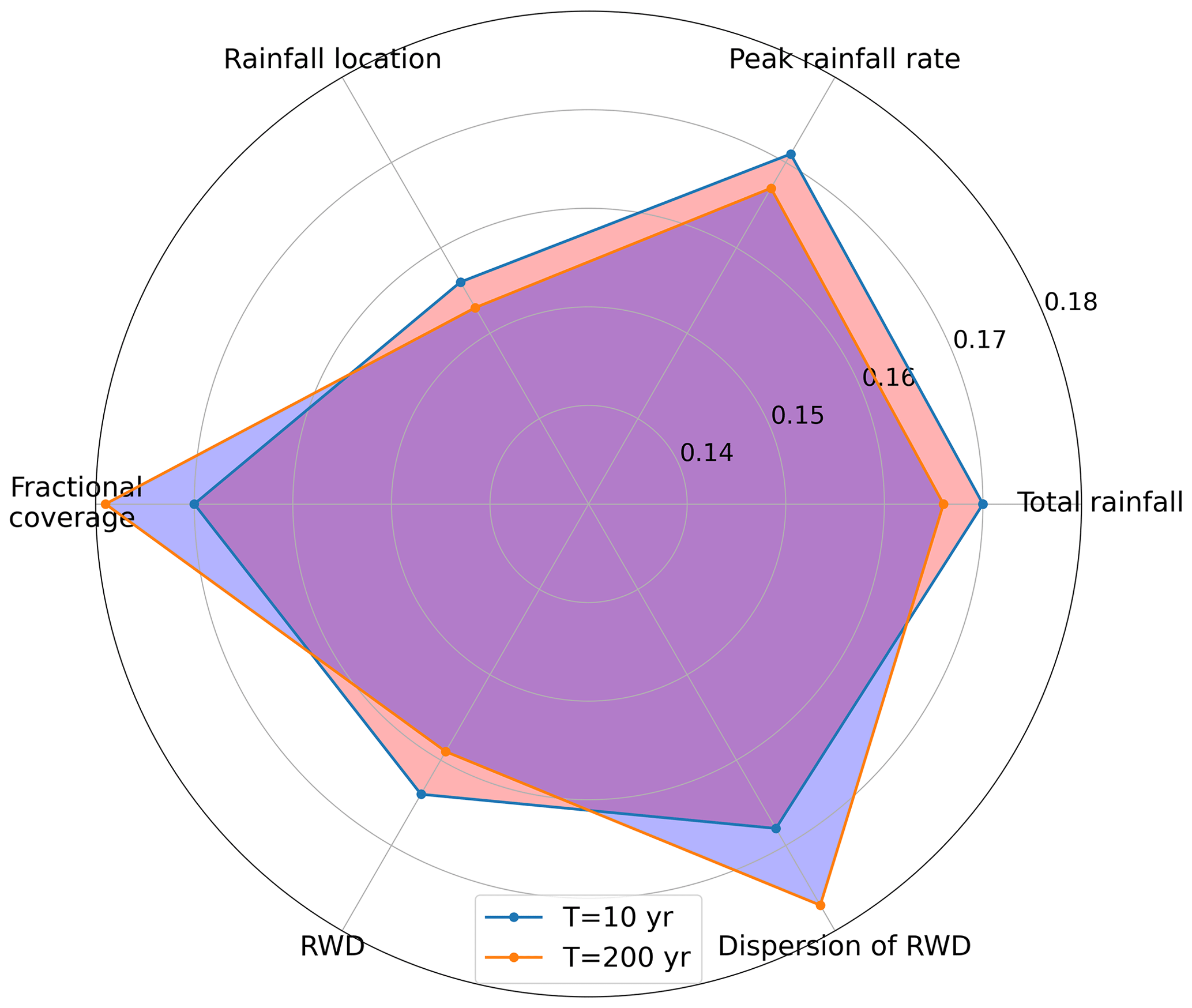
Figure 8 Feature importance analysis of RF model for space–time rainfall structure and 10-year (red) and 200-year (blue) flood peaks.

3.3.2 Rainfall return period vs. flood return period

In conventional design storm/flood practices, the return period of rainfall and peak discharge is often assumed to be equivalent (Rahman et al., 2002). Under the SST framework, we can examine this assumption (Wright et al., 2014a). At the 14.3 km² basin scale, for each SST realization containing 100 rainfall scenarios with a return period from 5 years up to 100 years, the peak discharge can be simulated and ordered. Flood frequency for return periods from 5 years up to 100 years is then estimated from the ordered peaks. We ran 30 SST realizations in total. Spearman's rank correlation of the two return periods is 0.5 (Fig. 9). The results quantitatively confirm that the assumption of a 1:1 return period equivalency between design storm and design flood cannot hold, even in a small highly urbanized watershed where the drainage network and rainfall structure play an important role in flood response. Similar results can be found between subbasins flood and DR-scale rainfall return periods (results not shown for the sake of brevity).

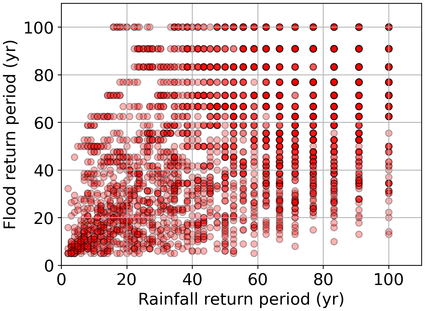
Figure 9 Scatterplot comparison return periods for rainfall and peak discharge for individual SST-based simulations.

3.3.3 Impact of rainfall spatial heterogeneity on flood responses

We also compared the simulated flood response resulting when rainfall is uniform over the watershed, rather than spatially distributed as in previous analyses (Fig. 4 and Table 2). Generally, flood peaks generated from uniform rainfall have lower peaks than from nonuniform rainfall. The difference increases with the return period. Under the 10-year return period, the shapes of the two hydrographs have similar upper and lower bounds (75 % and 25 % quantiles). The median flood peak using nonuniform scenarios is 22 % higher than the uniform scenarios. Under the 200-year return period, the hydrograph resulting from nonuniform rainfall is much peakier than the uniform SST scenarios, with higher upper and lower bounds. The lower bound of hydrograph by nonuniform SST scenarios is close to the median hydrograph of uniform SST scenarios.

Table 2 The median flood peak reductions using spatially uniform and spatially distributed rainfall.

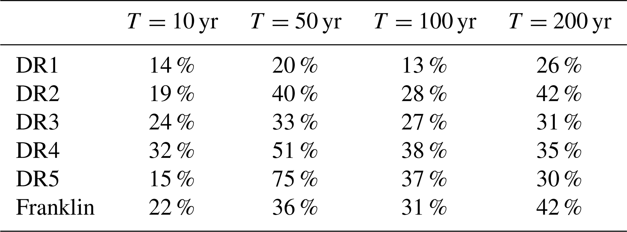
The impact of rainfall spatial heterogeneity among the five subwatersheds is different. DR1, with a basin scale of 1.32 km² and located in the northwest boundary of the watershed, was the least impacted by rainfall spatial distribution for all return periods. In DR2, on the other hand, which is similar in drainage area to DR1, the flood peak increased by 46 % for the 200-year return period. For DR3 and DR4, the spatial heterogeneity of rainfall contributes more to the flood peaks in DR4 than in DR3. The most striking difference in flood peaks is in DR5 for the 50-year return period. The difference in flood magnitude is 75 %. As mentioned above, DR5 is the sub-basin with the least detention-controlled area. This finding is likely tied to the complex relationship between space–time rainfall structure and the drainage network. We can thus conclude that the spatial heterogeneity of rainfall can increase flood peaks dramatically under both small and large return periods. The impact increases with the return period. This result shows that the assumption of spatially uniform rainfall will underestimate flood frequency.

4 Summary and conclusions

This paper addresses the problem of the impacts of short-duration rainfall variability on hydrologic response in the small urbanized watershed. By coupling a high-resolution radar rainfall data set and stochastic storm transposition (SST) with the GSSHA distributed physics-based model (see also Wright et al., 2014a; Zhu et al., 2018), the relationships between rainfall spatiotemporal structure and urban flood response are examined. The main findings are as follows:

1. The flood frequency distributions for subwatersheds within the highly urbanized 14.3 km² Dead Run watershed demonstrate the complexities of flood response for both short and long rainfall return periods. For 3 h extreme storms, the large variability of flood magnitude shows a pronounced role of rainfall space–time structure in flood production. This calls into question the common design storm assumption of spatially uniform rainfall. The response time is less affected by rainfall structure and appears to be more closely associated with the basin scale and drainage network features.

2. The spatial heterogeneity of flood frequency over the 14.3 km² watershed is striking for the 100-year return period. The intercomparison between subwatersheds shows that the impact of impervious area decreases with increasing return periods. For the 100-year return period, storm events that produce the same peak discharge return period at the basin outlet can be the result of very different upstream flood responses, even in a small-scale watershed.

3. The relationship between the space–time structure of rainfall and flood response is complex. For smaller and more frequent rainfall events, flood peaks are more closely linked to the temporal features of rainfall (total rainfall and peak rainfall rate). For extreme storms, the maximum discharge is closely linked to the spatial structure of rainfall (storm core coverage). This finding is broadly consistent with Peleg et al. (2017) and Zhu et al. (2018), despite the very different drainage scales considered in those studies. There is no significant correlation between rainfall peak, total rainfall and flood peaks, implying an important role of surface properties in urbanized watersheds. Similar to Wright et al. (2014a), this comparison calls into question the conventional design storm assumption of a 1:1 equivalency between rainfall and flood peak return periods.

4. The spatial heterogeneity of rainfall is a key driver of flood response across scales. Relative to spatially uniform rainfall, spatially distributed rainfall can increase flood peaks by 50 % on average at the watershed outlet and its subwatersheds for both small and large return periods. This finding is broadly consistent with prior results at much larger scales in an agricultural setting (Zhu et al., 2018) and suggests both spatial and temporal rainfall distributions need to be considered in flood frequency analyses, even in relatively small urban watersheds. This study also implies that the drainage network substantially alters the impact of rainfall characteristics on runoff.

Coupling the GSSHA model and SST-based rainfall frequency analysis, this study provides an effective approach for regional flood frequency analysis for urban watersheds. Some idealized assumptions used in conventional methods are questioned. The approach can be used to explore the dominant control on the upper tail of urban flood peaks, without many of the limiting assumptions associated with design storm methods. The study area could be extended in future work with larger basin scales and by manipulating the spatial heterogeneity of basin characteristics within GSSHA or other similar modeling systems.

Appendix A

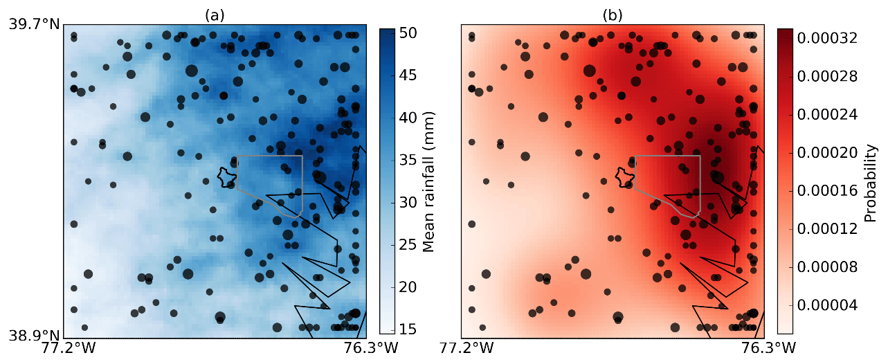
Figure A1 Maps of mean storm total rainfall (a) and probability of storm occurrence (b) for the 200 storms in the 3 h storm catalog. (The black dots indicate the locations of rainfall centroids.)

Figure A2 Composite map of rainfall distribution for the 10-, 50-, 100- and 200-year return periods.

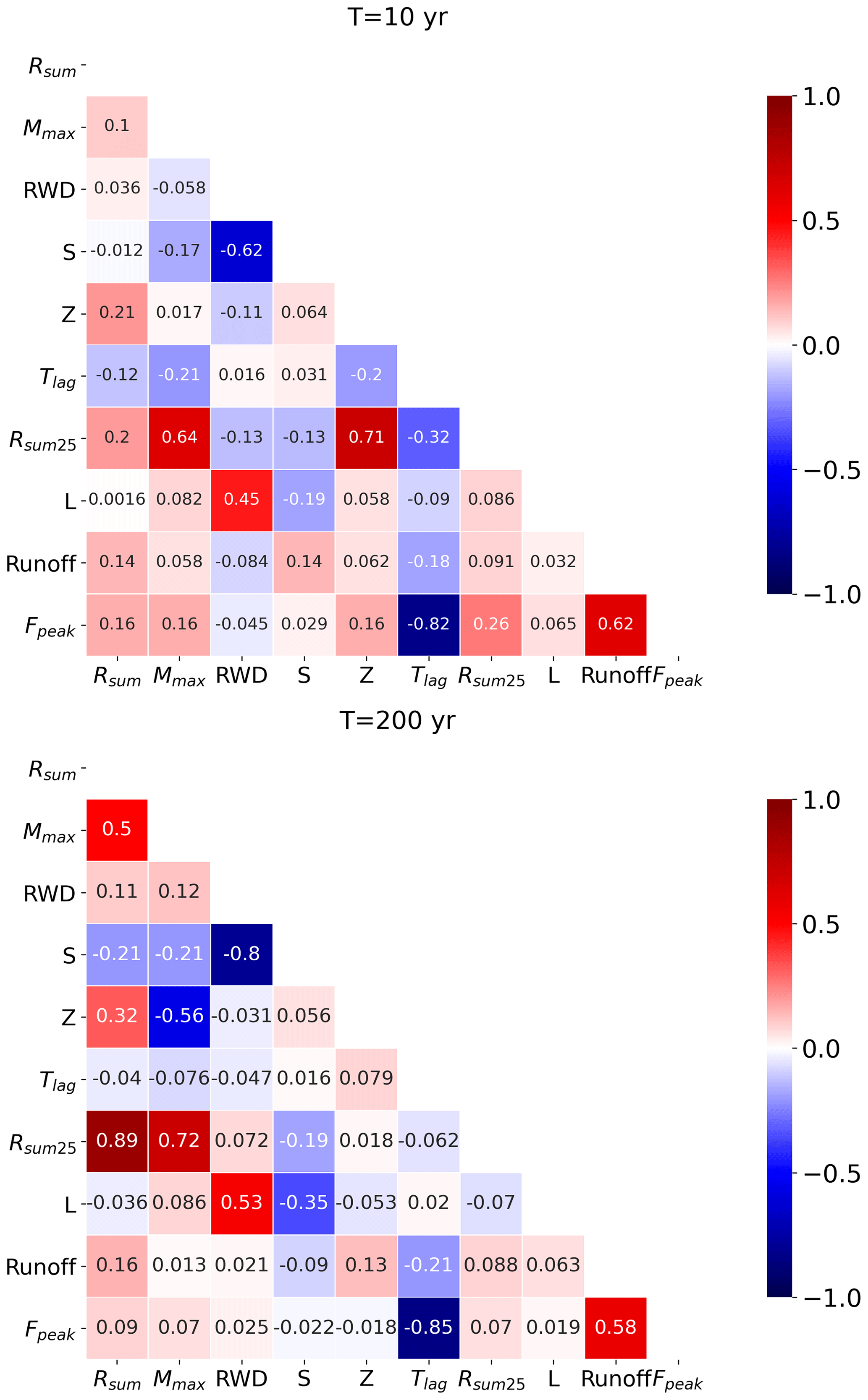
Figure A3 Correlation between space–time rainfall structure and flood responses at Franklintown under 10- and 200-year return periods.

Figure A4 The parameter tuning process of the RF model (using RMSE as an example).