Deep learning for automated river-level monitoring through river-camera images: an approach based on water segmentation and transfer learning

River-level estimation is a critical task required for the understanding of flood events and is often complicated by the scarcity of available data. Recent studies have proposed to take advantage of large networks of river-camera images to estimate river levels but, currently, the utility of this approach remains limited as it requires a large amount of manual intervention (ground topographic surveys and water image annotation). We have developed an approach using an automated water semantic segmentation method to ease the process of river-level estimation from river-camera images. Our method is based on the application of a transfer learning methodology to deep semantic neural networks designed for water segmentation. Using datasets of image series extracted from four river cameras and manually annotated for the observation of a flood event on the rivers Severn and Avon, UK (21 November–5 December 2012), we show that this algorithm is able to automate the annotation process with an accuracy greater than 91 %. Then, we apply our approach to year-long image series from the same cameras observing the rivers Severn and Avon (from 1 June 2019 to 31 May 2020) and compare the results with nearby river-gauge measurements. Given the high correlation (Pearson's correlation coefficient >0.94) between these results and the river-gauge measurements, it is clear that our approach to automation of the water segmentation on river-camera images could allow for straightforward, inexpensive observation of flood events, especially at ungauged locations.

1 Introduction

Fluvial flood forecasting systems often deploy hydrodynamic inundation models to compute water level and velocity in the river and, when the storage capacity of the river is exceeded, in the floodplain (e.g. Flack et al., 2019). Simulation library approaches using pre-computed hydrodynamic model solutions are also becoming more common for near real-time flood mapping (e.g. Speight et al., 2018). Observations of fluvial floods are key to model improvement, both to improve forecasts during the event via data assimilation (e.g. Ricci et al., 2011; García-Pintado et al., 2013, 2015; Di Mauro et al., 2021; Cooper et al., 2019) and to identify model shortcomings and improvements in post-event analysis (e.g. Werner et al., 2005). Water-level observations are often easier to obtain than streamflow observations, as they do not require any information about the rating curve. Furthermore, several studies have demonstrated their utility for calibration of hydrological models (e.g. van Meerveld et al., 2017; Seibert and Vis, 2016).

The main types of water-level observations possible with current technologies include ground-based and remote-sensing techniques. River gauges allow continuous monitoring of river levels at point locations. However, their measurements may not be valid if the gauge is overwhelmed in an extreme flood. The network of river gauging stations is declining globally (The Ad Hoc Group et al., 2001; Mishra and Coulibaly, 2009; Global Runoff Data Center, 2016). Consequently, many flood-sensitive areas are ungauged or must be studied through river gauges that can be located several kilometres away (e.g. Neal et al., 2009), so they cannot accurately describe the local situation.

Satellite and airborne images can be used to derive flood extents and, when combined with a digital elevation model (DEM), water levels along the flood edge (Grimaldi et al., 2016). These images can be obtained using optical sensors or synthetic aperture radar (SAR). Satellite and airborne optical techniques are hampered by their daylight-only application and their inability to map flooding beneath clouds and vegetation (Yan et al., 2015). On the other hand, SAR images are unaffected by cloud and can be obtained day or night. Thus, their use for flood mapping in rural areas is well established (e.g. Mason et al., 2012; Giustarini et al., 2016). In urban areas, shadow and layover issues make the flood mapping more challenging (e.g. Mason et al., 2018; Tanguy et al., 2017). In addition, SAR satellite overpasses are infrequent (at most once or twice per day, depending on location), so it is uncommon to capture the rising limb of the flood (Grimaldi et al., 2016).

Unmanned aerial systems (UASs) are an emerging technology increasingly being used for river observations (Tauro et al., 2018). However, UAS deployment is subject to civil aviation restrictions (e.g. Civil Aviation Authority, 2020). Furthermore, there is a balance between instrument payload and the need to land and refuel. Images are subject to UAS drift and require complex orthorectification (Perks et al., 2016).

Several studies have already attempted to use videos and still-camera images in order to observe flood events. Surface velocity fields can be computed using videos (e.g. Muste et al., 2008; Le Boursicaud et al., 2016; Creutin et al., 2003; Perks et al., 2020). Still images can be used to observe the water levels, either manually (e.g. Royem et al., 2012; Schoener, 2018; Etter et al., 2020) or automatically, for example by considering image processing edge detection techniques (Eltner et al., 2018). Under the right conditions, these automated water-level estimation techniques can provide good accuracy with uncertainties of only a few millimetres (Gilmore et al., 2013; Eltner et al., 2018). However, the performance of these approaches lacks portability (Eltner et al., 2018).

There have been a number of citizen science projects that investigated the use of crowd-sourced observations of river level (e.g. Royem et al., 2012; Lanfranchi et al., 2014; Etter et al., 2020; Lowry et al., 2019; Walker et al., 2019; Baruch, 2018). However, in our paper, the aim is to rely on “opportunistic data” (Hintz et al., 2019) from an existing network of river cameras to observe flood events. River cameras typically continuously broadcast live images from waterways. The cost of installation and maintenance of such cameras is low as they only rely on the availability of electricity through a power grid or (backup) batteries, and the upload of the images can be organised through standard and/or mobile broadband. Many of these cameras are installed at ungauged locations (Vetra-Carvalho et al., 2020b; Perks et al., 2020; Lo et al., 2015), and they have become a common tool for the monitoring of rivers for many private (e.g. fishing, tourism and boating) and public (flood prevention and river management) purposes. Thus, the use of existing cameras could offer a good coverage of the river network.

By extracting the location of water-filled pixels from a stream of river-camera images (water segmentation), it becomes possible to analyse flood events happening within the field of view of a camera. Most attempts that have tried to tackle the problem of automated water detection in the context of floods have been realised through the histogram analysis of the image (Filonenko et al., 2015; Zhou et al., 2020) unless the dynamic aspect of the video feed can be exploited (e.g. 25fps in Mettes et al., 2014) or the camera is set to observe a specific gauge or ruler (Pan et al., 2018), which is not the case for the river cameras used in this work (1 frame per hour). These algorithms remain sensitive to luminosity and water reflection problems (Filonenko et al., 2015). Deep learning approaches have been applied to flood detection using river cameras (Lopez-Fuentes et al., 2017; Moy de Vitry et al., 2019). However, current flood-related studies using river-camera images are limited because the observations made on the stream of images must be annotated manually (Vetra-Carvalho et al., 2020b). An accurate, manual annotation of such images is a long and tedious process that compels the analyst to narrow the scope (number of images considered) of the study.

Over the last decade, transfer learning (TL) techniques have become a common tool to try to overcome the lack of available data (Reyes et al., 2015; Sabatelli et al., 2018). The aim of these techniques is to repurpose efficient machine learning models trained on large annotated datasets of images to new related tasks where the availability of annotated datasets is much more limited (see Sect. 2 for more details). Vandaele et al. (2021) successfully analysed a set of TL approaches for improving the performance of deep water segmentation networks by showing that they could outperform water segmentation networks trained from scratch over the same datasets. This paper builds on the work of Vandaele et al. (2021) and studies the performance of these water segmentation networks trained using TL approaches for the automation of river-level estimation from river-camera images in the context of flood-related studies. In particular, this work uses water segmentation networks trained using TL approaches in order to carry out novel experiments realised with new river-camera datasets and metadata that consider the use of several methods to extract quantitative water-level observations from the water-segmented river-camera images.

Section 2 motivates and details the approach that was used to develop the river-level estimation method presented in this work. Section 3 presents and analyses the results of the experiments performed with this approach. Finally, Sect. 4 provides conclusions.

2 Transfer learning for water segmentation and river-level estimation

This section details the approach that was used to tackle the problem of river-level estimation from river-camera images. Section 2.1 provides explanations regarding the computer vision and deep learning concepts that were used in this work. Section 2.2 details how the problem of water segmentation is tackled. Section 2.3 explains how the water segmentation can be used to estimate river levels.

2.1 Definitions

Three concepts need to be introduced to understand the method presented in this work: water segmentation (Sect. 2.1.1), deep learning (Sect. 2.1.2) and transfer learning (Sect. 2.1.3). These explanations are kept short and oriented towards the main goal of this work. We refer the interested reader to additional information in computer vision and deep learning literature (e.g. Goodfellow et al., 2016; LeCun et al., 2015; Szeliski, 2010).

2.1.1 Water segmentation for water-level estimation

In this work, the problem of river-level estimation is tackled through the use of automated semantic segmentation algorithms applied to river-camera images. We focus on automated river and water semantic segmentation. As shown in Fig. 1, a water semantic segmentation algorithm will associate a Boolean variable 1 (flooded)$/$0 (unflooded) to each pixel of an RGB image, expressing whether or not there is water present in the pixel. The Boolean mask will thus have as many pixels as the RGB image.

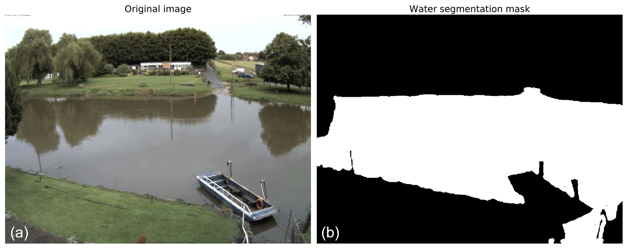
Figure 1 Example of a water segmentation mask (a) for a river-camera image (b). The mask corresponds to a pixel-wise labelling of the original images between flooded pixels (in white) and unflooded pixels (in black), expressing whether or not there is water present in the pixel.

While water segmentation masks do not allow for a direct estimation of the river level, producing an automated water segmentation algorithm is a major milestone in order to use river-camera images for river-level estimation. Section 2.3 details how the water segmentation masks can be used to estimate the river levels.

2.1.2 Deep learning for automated water segmentation

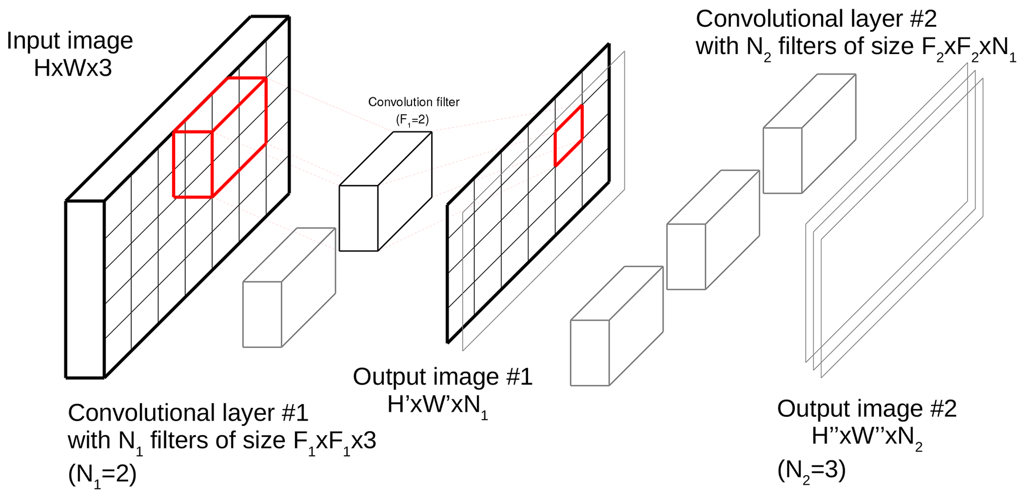
As for most image-processing-related tasks, recent advances in optimisation, parallel computing and dataset availability have allowed deep learning methods, and specifically deep convolutional neural networks (CNNs), to bring major improvements to the field of automated semantic segmentation (Guo et al., 2018). CNNs are a type of neural network where input images are processed through convolution layers. As shown in Fig. 2 for convolutional neural networks, an image is divided into square sub-regions (tiles) of size F×F that can possibly overlap. The image is processed through a series of convolutional layers. A convolutional layer is composed of filters (matrices) of size $F\times F\times C_i$, where C_i is the number of channels of the input image at layer i. For each filter of the convolutional layer, the filter is applied on each of the tiles of the image by computing the sum of the Hadamard product (element-wise matrix multiplication) – also called a convolution in deep learning – between the tile and the filter (Strang, 2019), which is then processed through an activation function (e.g. ReLU (Nair and Hinton, 2010), sigmoid or identity function). If the products of the convolution operations are organised spatially, the output of a convolutional layer can be seen as another image, which itself can be processed by another convolutional layer; if a convolutional layer is composed of N filters, then the output “image” of this convolutional layers has N channels. CNN architectures vary in number of layers and choice of activation function but also in terms of additional layers. Typically, SoftMax layers are added at the end of categorisation or classification tasks (such as semantic water segmentation) to normalise the last C_i channels into a probability distribution of C_i categories or classes. Pooling layers are often used to reduce the dimension of a layer by computing the maximum (max-pooling) or average (average-pooling) of partitions (non-overlapping contiguous regions) of size P×P of the input image.

During the training of the networks, the weights of the filters (the matrix values) are optimised. The idea is that the filters will converge along the convolutional layers towards weights, making the input image more and more meaningful for the task at hand.

Figure 2 Example of convolution layers inside a neural network.

2.1.3 Transfer learning

Inductive transfer learning (TL) is commonly used to repurpose efficient machine learning models trained on large datasets of well-known problems in order to address related problems with smaller training datasets. Indeed, water segmentation networks are typically trained on small datasets composed of 100–300 training images (Lopez-Fuentes et al., 2017; Steccanella et al., 2018; Moy de Vitry et al., 2019), while more popular problems can be trained on datasets composed of more than 15 000 images (e.g, Caesar et al., 2018; Zhou et al., 2017). In many cases, using inductive TL approaches for the training of CNNs instead of training them from scratch with randomly initialised weights allows improvement in the network performance (Reyes et al., 2015; Sabatelli et al., 2018).

For a typical supervised machine learning problem, the aim is to find a function $f:X\to Y$ from a dataset $B=\mathit{\left\{}\right(x_i,y_i{)}_{i=\mathrm{1}}^N:x_i\in X,y_i\in Y\mathit{\}}$ of N input–output pairs such that the function f should be able to predict the output of a new (possibly unseen) input as accurately as possible. The set X is called the input space and Y the output space.

With TL, the aim is to also build a function $f_{\mathrm{t}}:X_{\mathrm{t}}\to Y_{\mathrm{t}}$ for a target problem with input space X_t, output space Y_t and a dataset B_t. TL tries to build f_t by transferring knowledge from a source problem s with input space X_s, output space Y_s and a dataset B_s.

Inductive TL (Pan and Yang, 2009) is the branch of TL related to problems where datasets of input–output pairs are available in both source (X_s,Y_s) and target (X_t,Y_t) domains and where the source and target input spaces are similar (X_s≈X_t) but not the output space (Y_s≠Y_t).

Note that the specific approach that is used to apply TL is presented in Sect. 2.2.

2.2 Transfer learning for deep water semantic segmentation networks

This section introduces the approach used for automated water segmentation as well as the different techniques and materials related to its development. Note that a part of the water semantic segmentation approach was presented in Vandaele et al. (2021). The aim of this work is to provide a perspective centred around the application of this method in hydrology. The method is applied on new relevant datasets and its relevance is evaluated in the context of water-level estimation. All the results presented in this paper are novel.

2.2.1 Network architectures and source datasets

For this study, two state-of-the-art CNNs for semantic segmentation (semantic segmentation networks) were considered.

The first network considered is ResNet50-UperNet (RU). This network is an UperNet network with a ResNet50 image classification network used as a backbone. ResNet50-UperNet was trained on the ADE20k dataset (Zhou et al., 2018). ResNet50 (He et al., 2016) is a typical CNN architecture used for image classification tasks (at the image level) that the UperNet architecture transforms into a semantic segmentation network. ADE20k is a dataset designed for indoor and outdoor scene parsing with 22 000 images semantically annotated with 150 labels, among which four are water-related labels (see Table 1).

Table 1 Labels related to water bodies, and the number of images that contain at least one pixel with the corresponding label.

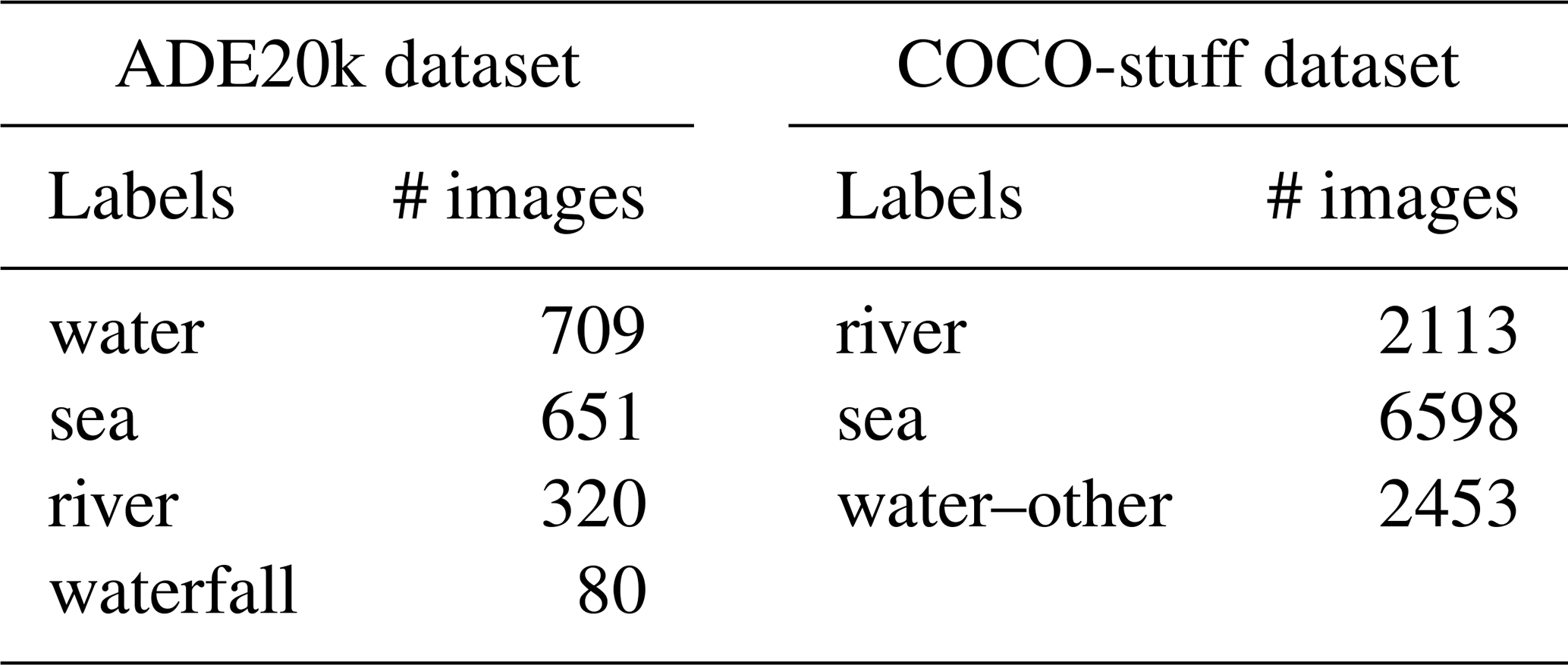
DeepLab (v3) is the second network that was considered. This network was trained and has produced state-of-the-art results on the COCO-stuff dataset (Chen et al., 2017). DeepLab also uses a ResNet50 network as a backbone network but performs the upsampling of the backbone's last layers by using atrous convolutions (Chen et al., 2017). COCO-stuff is a dataset made of 164 000 images semantically annotated with 171 labels, among which three are related to water objects (see Table 1).

2.2.2 Target datasets for water semantic segmentation

In order to apply transfer learning to the networks trained on the source problems, two different target datasets were considered.

• LAGO (named after the first author of the study presented in Lopez-Fuentes et al., 2017) is a dataset of RGB images with binary semantic segmentation of water masks. The dataset was created through manual collection of camera images having a field of view capturing riverbanks. The big advantage of this dataset is that the images are directly for river segmentation (Lopez-Fuentes et al., 2017). It is a dataset made of 300 images with 225 used in training.

• WATERDB is a dataset of RGB images with binary semantic segmentation of water and not-water labelled pixels that was created by Vandaele et al. (2021) through the aggregation of images containing label annotations related to water bodies coming from the ADE20k (Zhou et al., 2017) (water, sea, river, waterfall) and the COCO-stuff (Caesar et al., 2018) (river, sea, water–other) dataset (see Table 1). The dataset is made of 12684 training images.

While LAGO is a dataset that is more directly related to the segmentation of river-camera images, it is also a dataset with a much smaller set of images than WATERDB. By choosing these two datasets, it is possible to determine if better results are obtained when transfer learning is applied to the networks over large datasets with images that are not always directly related to the segmentation of water on river-camera images, or conversely if better results are obtained by applying transfer learning to the networks over smaller but more relevant datasets.

2.2.3 Applying transfer learning to train the networks

In Vandaele et al. (2021), the most successful approach considered for applying transfer learning to the semantic segmentation networks is fine-tuning. With fine-tuning, the filter weights obtained by training the network over the source problem are used as initial weights for training the network over the target problem.

The semantic segmentation networks that were chosen are addressing semantic segmentation problems with 171 (COCO-stuff) and 150 (ADE20k) labels (see Sect. 2.2.1) and use a SoftMax layer (see Sect. 2.1.2) to perform their segmentation, which means that their last layer has as many filter as there are labels. However, the water semantic segmentation problem is a binary segmentation problem with only two labels: water or not-water. In practice, this means that the dimensions of the last output layer of the source semantic segmentation networks and the target semantic segmentation networks might not be of the same size and will have a different number of filters. In consequence, it is not possible to use the weights of the last layer of the source network to initialise the weights of the last layer of the target network. This is why two fine-tuning strategies were considered in Vandaele et al. (2021).

• WHOLE: fine-tuning the entire target network with all the initial weights of all layers equal to the weights of the source network except for a random initialisation of the last binary output layers.

• 2STEPS: the last layer of the target network (with random initialisation) is retrained first with all the other layers frozen to the weights of the source network layers. Once the last layer is retrained, the entire target network is fine-tuned.

2.2.4 Networks retained for the experiments

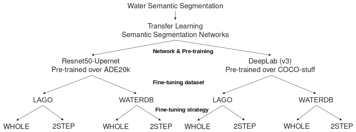
The discussion so far in Sect. 2.2 has presented different types of deep-learning-based approaches to tackle the automated water segmentation problem: CNN architecture, source and target datasets, as well as fine-tuning strategies. In particular, it has considered two network architectures pre-trained over specific datasets (ResNet50-UperNet pre-trained over ADE20k and DeepLab (v3) pre-trained over COCO-stuff) and two fine-tuning strategies (WHOLE or 2STEPS) applied on two different datasets (LAGO or WATERDB). This means that eight different network configurations were trained (see Fig. 3).

Figure 3 Model configurations used with the TL methodology.

As explained in Vandaele et al. (2021), the training used 300 epochs in order to ensure full convergence for all the networks. The initial learning rate value for the fine-tuning was 10 times smaller than its recommended value (0.001) in order to start with less aggressive updates. The other parameters (loss, update schedule and batch size) were chosen as recommended by the authors of the networks (Zhou et al., 2018; Chen et al., 2017). Both authors implemented their network using the PyTorch library.

2.3 River-level estimation using water segmentation

The deep learning methodology presented in Sect. 2.2 allows the estimation of a water mask from a river-camera image. However, as explained in Sect. 2.1, it is not possible to directly extract the water level from the water masks. Hence, this section details two approaches that can be used to extract river levels from water masks.

2.3.1 Static observer flooding index (SOFI)

The experiments presented in this work use the static observer flooding index (SOFI) to track water-level changes. Moy de Vitry et al. (2019) introduced the SOFI to extract flood-level information from a deep semantic segmentation network trained from scratch on an image dataset annotated with water labels. The SOFI is related to the percentage of pixels in the image that are estimated as water pixels by the network as

$$\begin{array}{}\text{(1)}& \text{SOFI}={\displaystyle \frac{\mathit{\#}{\text{Pixels}}_{\text{Flooded}}}{\mathit{\#}{\text{Pixels}}_{\text{Total}}}}.\end{array}$$

This non-dimensional index allows the authors to monitor the evolution of water levels in their datasets and can be computed on the entire water mask or only a sub-region.

2.3.2 Landmark-based water-level estimation (LBWLE)

The landmark-based water-level estimation (LBWLE) developed with this work aims at estimating the water level by using the landmark classification information. As suggested in Fig. 4, this algorithm relies on landmark locations (points) chosen specifically for a camera (e.g. near the river or in areas likely to get flooded) and for which the height is available from a ground survey.

LBWLE estimates the water-level height $\widehat{w}$ as the average of a lower bound landmark height h_lb and an upper bound landmark height h_ub, which is $\widehat{w}=\frac{h_{\mathrm{lb}}+h_{\mathrm{ub}}}{\mathrm{2}}$.

However, simply considering the lower bound lb as the highest flooded landmark and the upper bound landmark ub as the lowest unflooded landmark could be problematic. Indeed, even if the water segmentation networks have relatively high segmentation accuracy, this algorithm needs to manage the possibility that landmarks with lower heights are estimated as unflooded while landmarks with higher heights might be estimated as flooded. This is why the LBWLE method uses the following approach.

Let $\widehat{F}\in [\mathrm{0},\mathrm{1}{]}^N$ be the estimated flood state of the N landmarks, sorted by increasing order of height h_i, and k be the index of the highest flooded landmark $k=max\mathit{\left\{}i\right|{\widehat{F}}_i=\mathrm{1},i=\mathrm{1},\mathrm{\dots },N\mathit{\}}$. If $U={\sum }_{i=\mathrm{1}}^k(\mathrm{1}-{\widehat{F}}_i)$ is defined as the number of unflooded landmarks between 1 and k, then the lower bound index lb is defined as lb $=\lceil k-U\frac{U}{k}\rceil$ and the upper bound ub is defined as ub = lb +1. With this algorithm, the idea is to first consider the lower bound index lb as the index of the highest landmark estimated as flooded, but switch to lower landmark indices depending on the percentage of unflooded landmarks between 1 and k. An example for the choice of the lower bound index using LBWLE is given in Fig. 4.

Figure 4 Example application of the LBWLE algorithm. The principle is that if some of the highest landmarks are estimated as flooded but some lower height landmarks are estimated as unflooded, then the true water level is likely lower than the height of the highest landmark estimated as flooded.

The estimated river-level height $\widehat{w}$ will then be estimated as the average between the heights of the landmarks defined as the lower and upper bounds $\widehat{w}=\frac{h_{\mathrm{lb}}+h_{\mathrm{ub}}}{\mathrm{2}}$. If no landmark is estimated as flooded, then the water level is set to $\widehat{w}=h_{\mathrm{1}}$ (the lowest water level measured), and if all the landmarks are estimated as flooded, then the water level is set to $\widehat{w}=h_N$ (the highest water level measured). Note that the accuracy of LBWLE is dependent on the annotated landmarks as it can only estimate the water level as the average height of two landmark heights.

2.3.3 Comparison of SOFI and LBWLE

When compared to the SOFI, water-level estimation using landmarks and LBWLE is at a disadvantage because of the necessary and time-consuming ground survey of the location observed by the camera. Furthermore, landmarks can mostly only be used when the river is out-of-bank, so the approach is not likely to capture drought events. However, the main advantage of this approach compared to SOFI is that it allows estimation of quantitative river levels in accepted units of length (e.g. metres). The SOFI values are dimensionless percentages and to convert them to a height measurement an appropriate scaling must be obtained by calibration with independent data.

3 Experiments

Two experiments were carried out in this study.

The first experiment, presented in Sect. 3.1, is designed to address the suitability of our approach for the automatic derivation of water-level observations using river-camera images and landmarks from a ground survey. Landmarks and associated manually derived water levels are available for a 2 week flood event (Vetra-Carvalho et al., 2020b). These data allow us to validate our LBWLE approach for water-level estimation in accepted units of length (metres) with co-located water levels estimated by a human observer.

With the second experiment, presented in Sect. 3.2, our approach is applied to larger, 1 year datasets of camera images that include a larger range of river flow rates and stages. This experiment allows us to better understand the suitability and robustness of the LBWLE and SOFI water-level measurements. However, manually derived co-located water levels are not available for this period, so the nearest available river-gauge data for validation was used instead. For some of the cameras, the nearest gauge is several kilometres away.

3.1 Application on a practical case for flood observation

3.1.1 River-camera datasets for a flood event on the river Severn and the river Avon

For this experiment, four different cameras located along the rivers Severn and Avon, UK, were considered: Diglis Lock (DIGL), Tewkesbury Marina (TEWK), Strensham Lock (STRE) and Evesham (EVES). The images capture a major flood event that occurred in the Tewkesbury area between 21 November and 5 December 2012. This is a well-observed and well-studied event (García-Pintado et al., 2015). Further information about the camera locations can be found in Vetra-Carvalho et al. (2020b).

The cameras are part of the Farson Digital Watercams (https://www.farsondigitalwatercams.com/, last access: 3 August 2021) network. The field of view of the cameras stays fixed (no camera rotation or zoom). The images were captured using a Mobotix M24 all-purpose high-definition (HD) web-camera system with 3MP (megapixels) producing 2048×1536 pixel RGB images. The images at our disposal were all watermarked, but a visual inspection of our results showed that those watermarks had near to no influence on the segmentation performance.

For each camera, ground surveys have previously been conducted in order to measure the topographic height of several landmarks within the field of view of the camera (Vetra-Carvalho et al., 2020b). Note that the number and spread of measured landmarks over the camera's field of view was constrained to locations that were accessible during the ground survey. For each camera, daytime hourly images (around nine per day) were retrieved and annotated by a human observer using the surveyed landmarks as a reference in order to estimate the water level as well as the accuracy of this estimation (Vetra-Carvalho et al., 2020b). This also means that for each landmark that was surveyed, it was possible to annotate the landmark with flood information. It is flooded if the water level is above the landmark's height; otherwise it is not. More details regarding the four datasets are given in Table 2. A sample image for each location, annotated with the measured landmarks, is given in Fig. 5.

An inspection of the datasets and results showed that the impact of camera movement was negligible. Machine-learning-based landmark detection algorithms (e.g, Vandaele et al., 2018) could have been used otherwise, but they are unnecessary in the context of this study.

Also note that this work focuses on a simple process relying on single pixel landmark locations annotated by Vetra-Carvalho et al. (2020b). The use of landmarked areas of multiple pixels sharing the same height could likely help to increase the detection performance and should be considered for optimal use of this landmark-based approach.

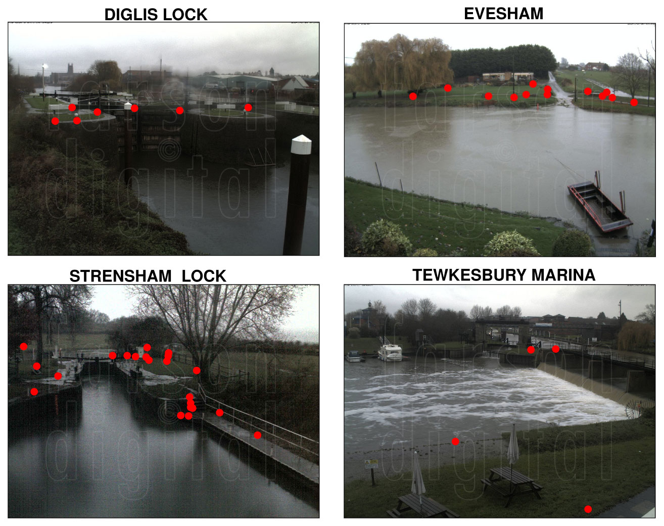
Figure 5 Sample camera image for each location with the measured landmarks annotated by red dots. Photo: Farson Digital Watercams.

Table 2 River-camera location and specific dataset information.

3.1.2 Evaluation protocol

As explained in Sect. 3.1.1, the images in the datasets used in these experiments are not annotated with binary masks that would allow the pixel-wise evaluation of the semantic segmentation networks. However, for our application, the landmark observations (Vetra-Carvalho et al., 2020b) provide the binary flooding information for some of the most relevant locations in the image. In consequence, the most relevant way to evaluate our approach is to consider it as a binary landmark classification problem and use the typical evaluation criteria related to binary classification (e.g. Gu et al., 2018; Bargoti and Underwood, 2017; Salehi et al., 2017). Note that these criteria are also commonly used in hydrology to evaluate the performance of flood modelling methods for flood-extent estimation (e.g. Stephens et al., 2014). Therefore, this experiment considers the set of criteria presented in Table 3 to describe the performance of our networks and also provides the corresponding contingency table. The contingency table was computed between the class labels of the landmarks estimated by a human expert examining of the images (Vetra-Carvalho et al., 2020b), and the class labels estimated by our semantic segmentation networks (pixels corresponding to the landmark locations in the images, estimated as flooded or unflooded).

Table 3 Metrics used to evaluate the algorithm's performance. A, B, C and D respectively correspond to true flooded (landmark flooded predicted as flooded), true unflooded (landmark unflooded predicted as unflooded), false flooded (landmark unflooded predicted as flooded) and false unflooded (landmark unflooded predicted as flooded).

As explained in Sect. 2.2, eight different network configurations were considered. For each network, the corresponding water segmentation masks of each image of each dataset were generated. The contingency table for the landmark classification for each dataset and each network was then computed separately.

3.1.3 Landmark classification results

The results are presented in Table 4. For the DIGL, EVES, STRE and TEWK datasets, the best approaches are the DeepLab networks trained on the LAGO dataset. Indeed, these networks are able to classify the landmarks with balanced accuracy (BA) of $\mathrm{0.95},\mathrm{0.97},\mathrm{0.91}$ and 0.95 respectively and they always obtain good scores for bias and false alarms (F). When comparing the corresponding bias (Table 4) to the proportion of flooded landmarks (Table 2), these best approaches (DeepLab networks trained on the LAGO dataset) tend to estimate slightly more flooded landmarks than expected. However, in comparison with the other networks, they tend to show the lowest false alarm rates (F) and have slightly lower performance for hit rates (H). This shows that they are less prone to overprediction than the other networks at the expense of a slightly higher number of false unflooded (B) landmark predictions.

On average, the DeepLab architecture pre-trained over COCO-stuff obtains better detection performance than the ResNet50-UperNet architecture pre-trained over ADE20k. The only criteria for which ResNet50-UperNet is competitive with DeepLab is the hit rate (H). This means that the networks tend to predict landmarks marked as flooded with an accuracy on par with DeepLab.

While 2STEPS and WHOLE fine-tuning strategies have very similar performance with BA, 2STEPS shows overall lower bias than WHOLE.

The networks fine-tuned over LAGO have a clear advantage over the ones fine-tuned over WATERDB. This difference is especially noticeable on two out of four datasets, mostly TEWK, but also STRE. For both STRE and TEWK datasets, fine-tuning the networks over WATERDB decreases the capacity of the network to detect the flooded landmarks. Table 2 shows that the TEWK dataset contains the largest number of flooded landmarks and STRE the second largest. Since the WATERDB dataset contains a larger proportion of images with small water segments (e.g. fountains, puddles, etc.), the networks fine-tuned over WATERDB have more difficulties generating large water segments than would be necessary for STRE and TEWK.

Given these observations, using the DeepLab network fine-tuned over the LAGO dataset with a 2STEPS strategy is the best configuration to use.

Table 4 Landmark detection results (for the metric meanings, see Table 3). For each location and each metric, the best network results are in bold. RU stands for the ResNet50-UperNet network.

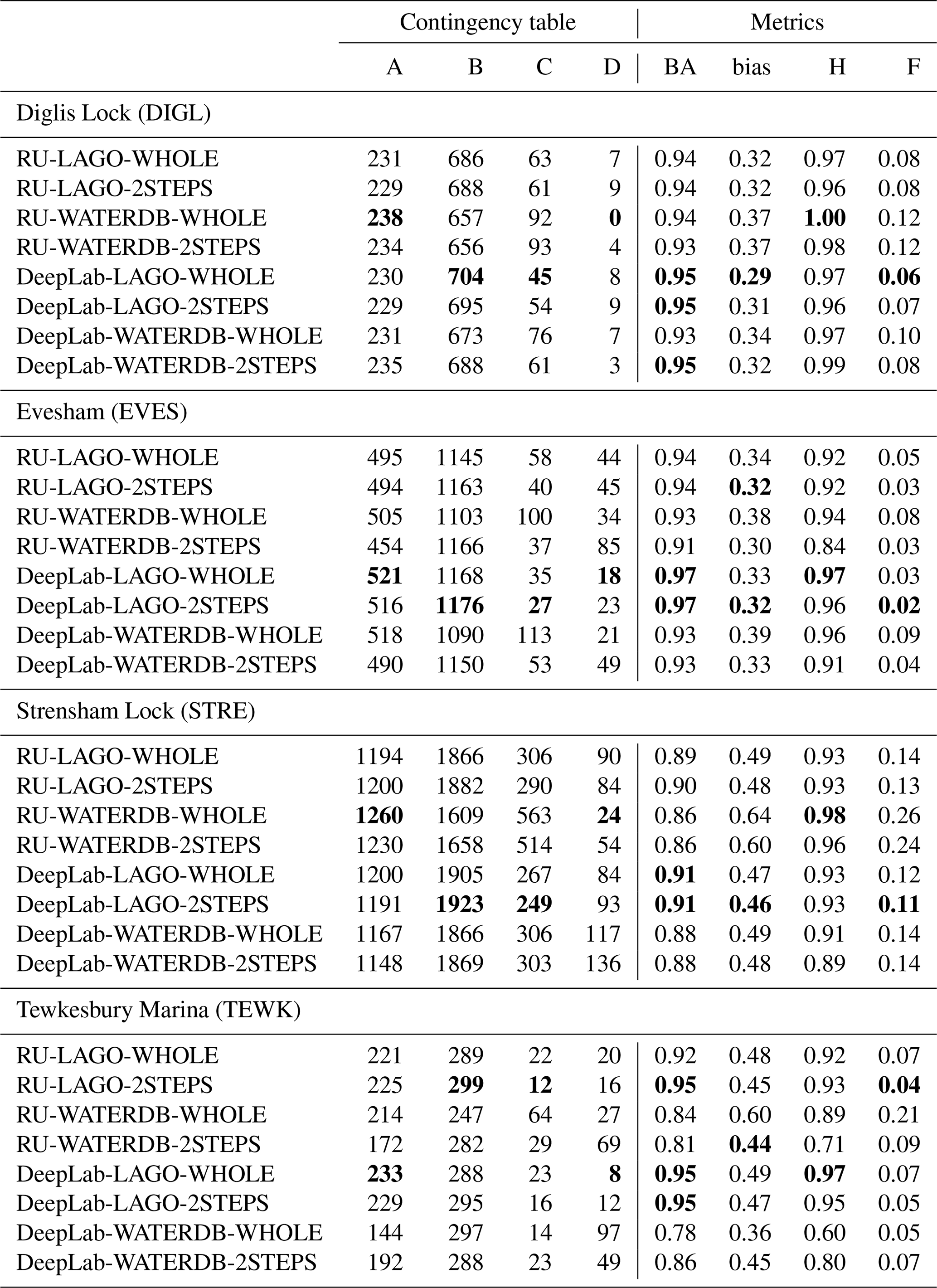
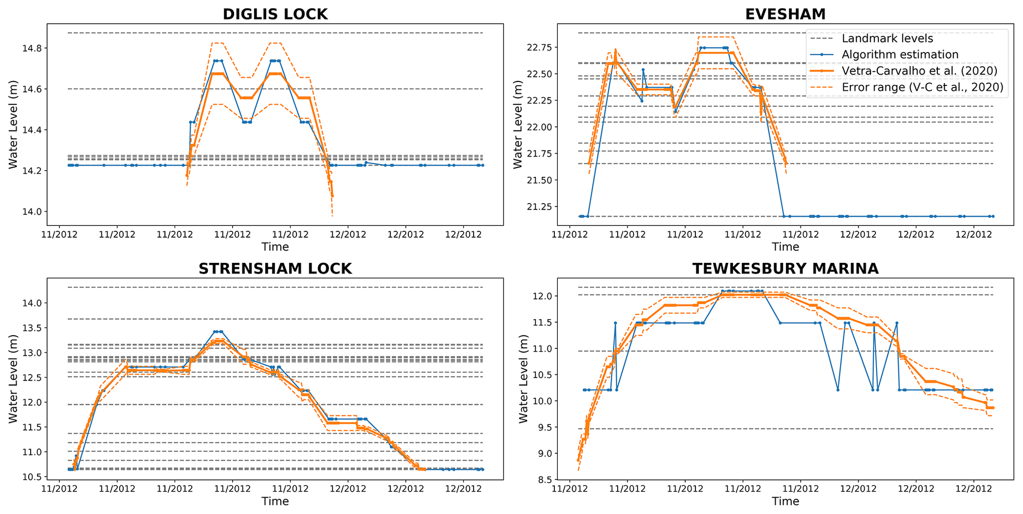
Figure 6 Comparison of the water-level estimation method using the DeepLab-LAGO-2STEPS network (in blue) and using the landmarks with the ground truth water levels directly extracted from the images (Vetra-Carvalho et al., 2020b) (in orange). The horizontal dashed lines correspond to the heights of the landmarks ground surveyed on these locations (see Sect. 3.1.1) that can be used as lower and upper bounds by the water-level estimation algorithm LBWLE (see Sect. 2.3.2). Note that the water-level estimation performed by manual examination of the images (Vetra-Carvalho et al., 2020b) was not always available outside of the flood event itself (Diglis Lock, Evesham and Strensham).

3.1.4 Estimating the water level using the landmark classification

Figure 6 shows the results of the LBWLE estimation method (see Sect. 2.3.2) applied on the best performing network (DeepLab-LAGO-2STEPS). For Diglis Lock, Evesham and Strensham, Fig. 6 shows that for the evaluated 2 week flood event period, LBWLE was able to give a good approximation of the manually estimated water level. Indeed, LBWLE's estimation and the water level estimated by a human observer almost always have the same landmarks as the lower and upper bounds, which is as close as LBWLE's performance can achieve as it is limited by the heights of the landmarks that were measured during the ground survey (the dotted lines in Fig. 6). Only a few estimation mistakes were made on the Tewkesbury Marina dataset; out of 138 images, only 5 estimation mistakes were made. Those mistakes were due to a landmark that was annotated on a platform close to a building. In this case, the networks stretched the unflooded segmentation area (related to the building) to the landmark location.

3.2 Performance evaluation for year-long water-level analysis

3.2.1 Year-long river-camera images datasets

For this experiment, the same camera locations as those used for the first experiment presented in Sect. 3.1.1 were considered. However, a different, longer 1 year period from 1 June 2019 to 31 May 2020 was used. According to a government report (Finlay, 2020), three major flood events occurred during this period. The first one, in November, was due to heavy rainfall at the start of the month (7–8 November), followed by additional heavy rainfall between 13 and 15 November. The second major event happened in the second half of December, with heavy rain pushing across the southern parts of England and lasting until the New Year 2020. Finally, the storms Ciara, Dennis and Jorge swept across the UK from 9 February 2020 to the early days of March. Additionally, heavy rainfall occurred between 10–12 June 2019.

Diglis Lock, Evesham, Strensham Lock and Tewkesbury Marina datasets have 3081, 3012, 3067 and 3147 images respectively. The difference in the number of images is due to minor technical camera problems making some images unavailable. The Diglis Lock and Tewkesbury Marina camera mounting positions, orientation and fields of view were changed in 2016 (Vetra-Carvalho et al., 2020b), so they are different from the first experiment (see Fig. 5). The new fields of view are presented in Fig. 7. The original RGB image size for these datasets is 640×480, which is a lower image resolution than in the first experiment. As the Diglis Lock and Tewkesbury Marina camera locations were changed, the corresponding landmarks used in the first experiment can not be considered for this experiment.

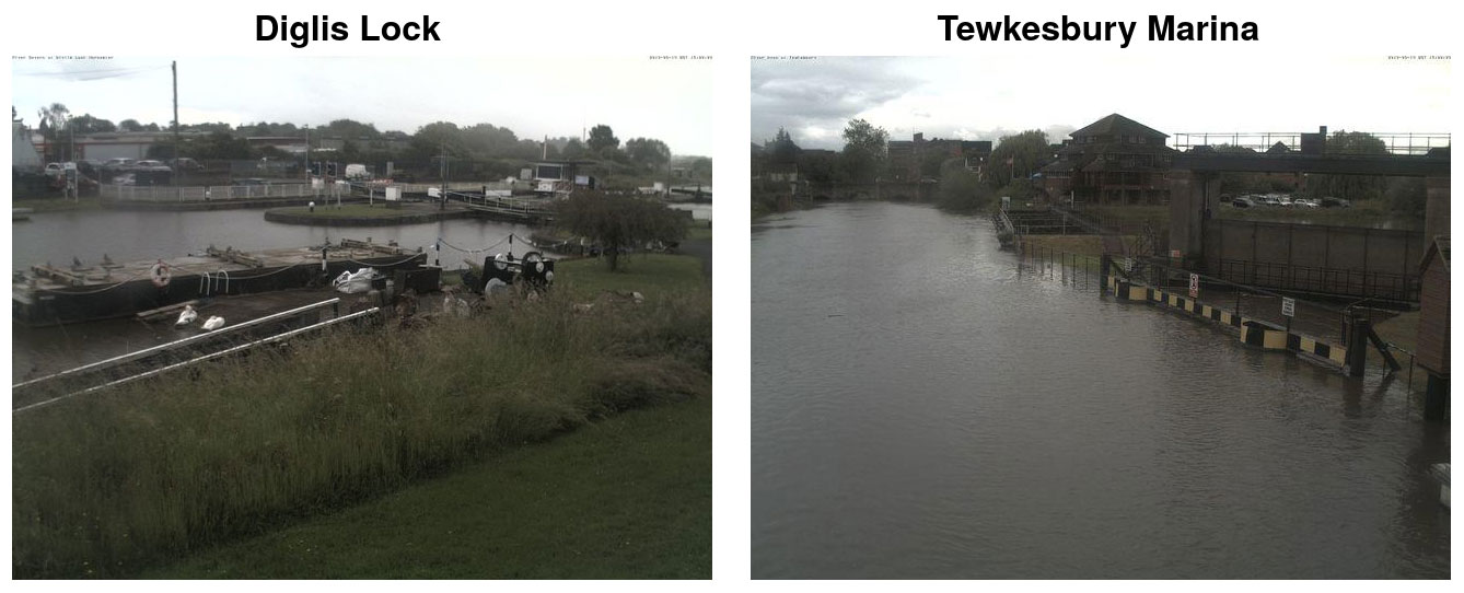
Figure 7 Fields of view from Diglis Lock and Tewkesbury Marina cameras for the period 2019–2020.

The water levels were not manually annotated on these year-long datasets. In order to evaluate the relevance of the algorithm presented in this paper on these datasets, water-level information coming from nearby river gauges available through the UK's Environment Agency open data API (Environment Agency, 2020) was used. The water-level information from the river gauges is not expected to reflect the exact situation observed at the camera location, but the water levels should be highly correlated. The locations of the gauges are given in Table 5 of Vetra-Carvalho et al. (2020b). The distance from the camera to their nearest river gauge ranges from 51 to 1823 m.

3.2.2 Evaluation protocol

Given that it is impossible to use the landmarks from the ground survey on two of the four cameras that were used in the first experiment and independent water-level information for validation is from nearby rather than co-located river gauges, the protocol developed for the first experiment (see Sect. 3.1.2) cannot be used. Hence, after applying the water semantic segmentation networks on the images, two experiments were designed.

1. Landmark-based water-level estimation analysis. For the images from the two locations for which the annotated landmark locations are still valid (Evesham and Strensham Lock), this experiment considers the correlation between the water-level measurements from the nearest river gauges and the water levels estimated by applying the LBWLE algorithm (see Sect. 2.3.2) on the water masks obtained by the water semantic segmentation networks.

   The correlation between N estimations of water levels, with w being the LBWLE estimation and g being the corresponding nearest river-gauge water-level measurement is computed using Pearson's correlation coefficient (Freedman et al., 2007), as defined in Eq. (2),

   $$\begin{array}{}\text{(2)}& \mathit{\rho }={\displaystyle \frac{{\sum }_i^N(w_i-\stackrel{\mathrm{‾}}{w})(g_i-\stackrel{\mathrm{‾}}{g})}{\sqrt{{\sum }_i^N(w_i-\stackrel{\mathrm{‾}}{w}{)}^{\mathrm{2}}}\sqrt{{\sum }_i^N(g_i-\stackrel{\mathrm{‾}}{g}{)}^{\mathrm{2}}}}},\end{array}$$

   where $\stackrel{\mathrm{‾}}{w}=\frac{\mathrm{1}}{N}{\sum }_i^N{w}_i$ and $\stackrel{\mathrm{‾}}{g}=\frac{\mathrm{1}}{N}{\sum }_i^N{g}_i$.

2. Full-image SOFI analysis. For each of the four locations, this experiment considers the Pearson's correlation coefficient between the water-level measurements obtained from the nearest river gauge and the SOFI (Moy de Vitry et al., 2019) computed on the segmented images. The SOFI is defined in Eq. (1).

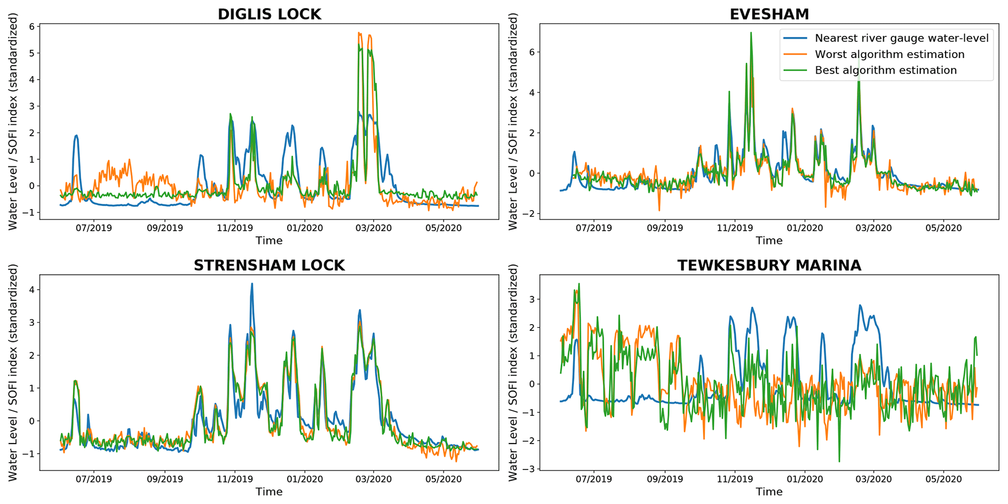
3.2.3 Landmark-based water-level estimation analysis

For the images from the two locations for which the annotated landmark locations are still valid (EVES and STRE), Table 5 shows the correlation between the nearest river-gauge water-level measurements and our water-level estimation using the LBWLE algorithm presented in Sect. 2.3.2. For these images, the networks that were trained on WATERDB obtain among the highest correlations. This is especially the case for the DeepLab networks. The DeepLab networks obtain higher correlations than the ResNet50-UperNet networks. The 2STEPS fine-tuning approach has a slight advantage over WHOLE fine-tuning. However, these differences stay relatively small as the camera location has a higher influence on the correlation.

The locations have a more significant influence over the results: the Strensham location always obtains higher correlations than Evesham. However, Table 4 (computed for the first experiment) shows that the Evesham landmarks get generally better detection results than the Strensham Lock landmarks. Considering the corresponding time evolution of the water levels in Fig. 8, it is possible to explain the highest correlations at Strensham Lock by the fact that the Evesham landmark heights do not allow tracking of the typical lower water levels when the river is in-bank, while the landmarks at Strensham Lock allow better tracking of the water level at lower heights.

In addition, as the river gauge used for Strensham Lock (Eckington Sluice) is 51 m away from the camera whereas the nearest river gauge to the Evesham camera is 1823 m away (Vetra-Carvalho et al., 2020b), it could be expected that the water levels extracted from the nearest river gauge at Strensham depict a more representative evolution of the water levels at Strensham Lock than the river gauge used for Evesham. Also, note that at Strensham, the lock can affect the water level.

Table 5 Pearson's Correlation Coefficients computed between the landmark-based water-level estimation and the water levels from the nearest river gauges on Evesham and Strensham Lock dataset.

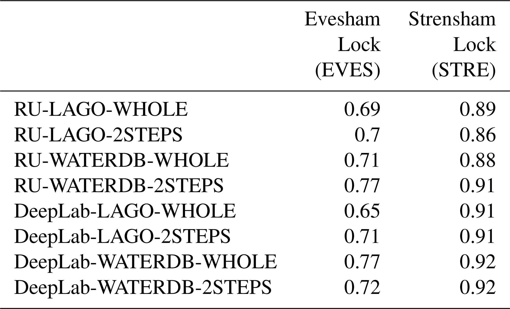
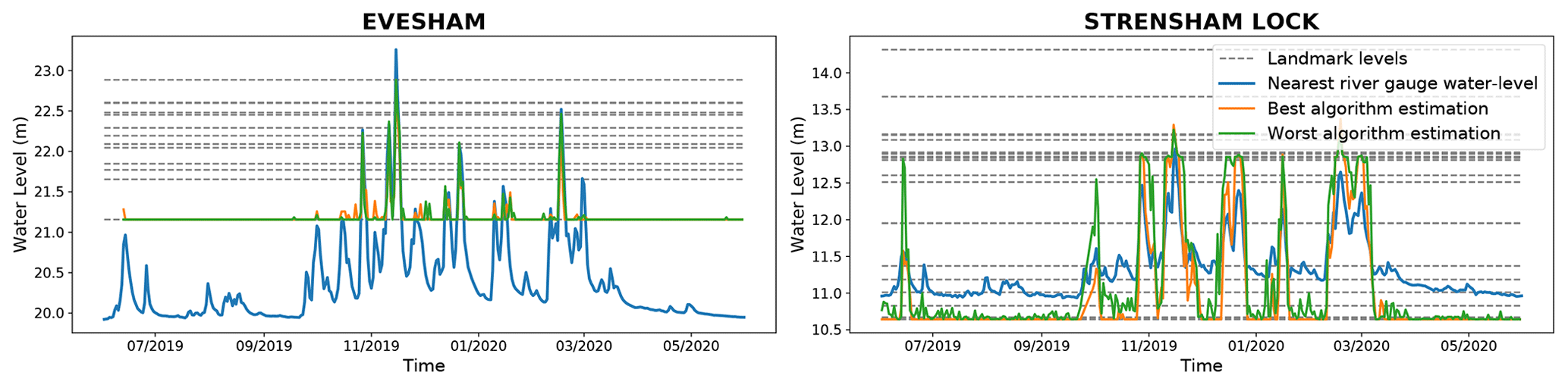
Figure 8 Evesham and Strensham Lock year-long water levels measured using landmark annotations in comparison with water levels from nearby river gauges. The best networks are DeepLab-WATERDB-WHOLE for Evesham and Strensham. The worst networks are RU-LAGO-WHOLE for Evesham and RU-LAGO-2STEPS for Strensham.

3.2.4 Full-image SOFI analysis

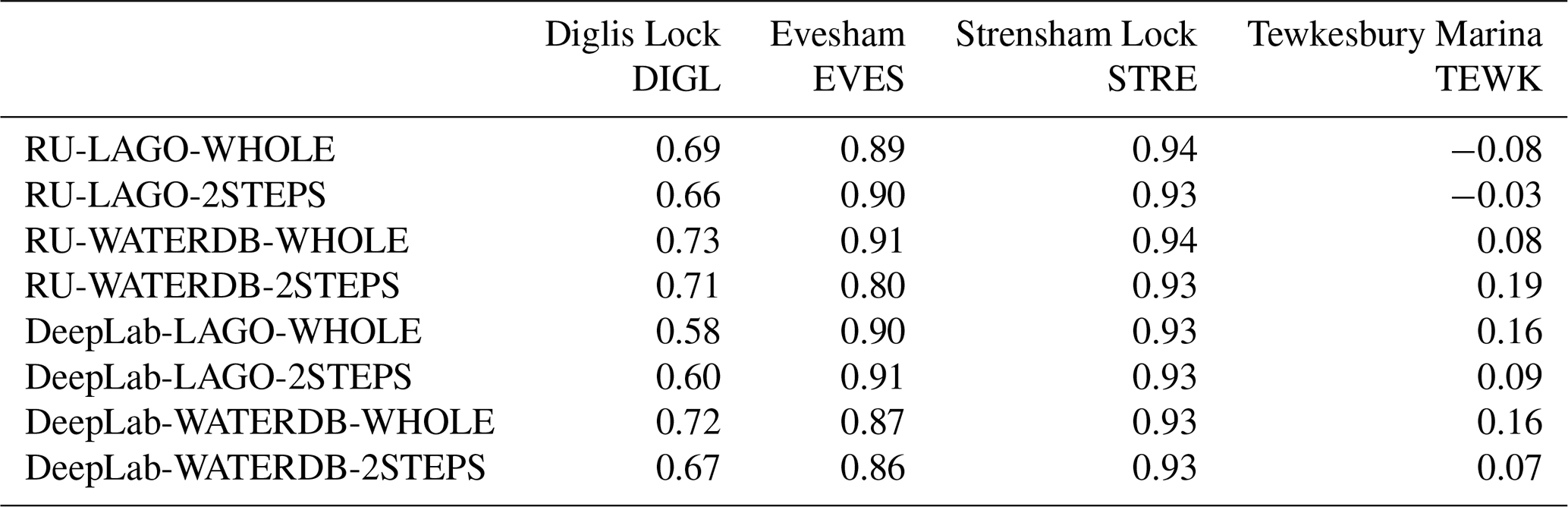
For each of the four cameras, Table 6 shows the correlation between the SOFI computed on the images using our segmentation method and the corresponding water levels from the nearest river gauges. Figure 9 shows the corresponding standardised water levels and the standardised SOFIs with the highest and lowest correlation with the water level, produced with the corresponding networks shown in Table 6. In this work, the term standardisation is used to describe the process of putting different variables on the same scale. In order to standardise the observed value x_i of a variable X, the standardisation process considers the difference of this observed value x_i with the mean (time-average) of the variable $\stackrel{\mathrm{‾}}{X}$ and divide this difference with the standard deviation of the variable σ(X). So, if $x_i^S$ is the standardised observed value corresponding to x_i, then $x_i^S=\frac{x_i-\stackrel{\mathrm{‾}}{X}}{\mathit{\sigma }\left(X\right)}$.

Table 6 shows that the correlations of the eight networks with the river-gauge water levels are relatively similar and that the difference between datasets is much more obvious. The lowest correlation on Strensham is higher than the highest correlation obtained on Evesham. The lowest correlation obtained on Evesham is higher than the highest correlation obtained on Diglis and the lowest correlation on Diglis is higher than the highest correlation on Tewkesbury. The correlation results are especially low for the Tewkesbury Marina location, where some correlations are close to zero or negative. For Strensham and Evesham, the correlations using the SOFI are higher than the correlations obtained when using the landmark information (see Table 5).

The higher correlations in Table 6 in comparison with Table 5 can be explained by examining the evolution of the water levels in Fig. 9. Figure 9 shows that the SOFI allows the algorithms to provide a better estimate of the water level when the river is in-bank than the landmark-based estimation. However, the estimates, when the water levels are low, stay fairly approximate and subject to small perturbations. Indeed, at low water level there are changes in the SOFIs that are not correlated with any particular event. By analysing the results on the Tewkesbury Marina dataset, where that phenomenon is the strongest, a visual inspection of the water segmentation results showed that the segmentation networks worked correctly. However, due to the new field of view of the camera and the configuration of the location, floods were not heavily increasing the number of water pixels in the image, and thus did not result in a large increase of the SOFI. The occlusion of some water segments in the image due to passage or mooring of boats could have a significant influence on the SOFI results, thus explaining the uncorrelated SOFI changes for this dataset. In all the locations, there are also smaller, noisy perturbations of the SOFI when the water level is low and steady. These perturbations are due to various, smaller-scale problems: occlusions by boats or changes in the lock configuration (there is a cable ferry at the Evesham location and the other locations are all locks), small segmentation errors or approximations from the segmentation algorithm. Besides, it is also likely that depending on the site configuration (e.g, the slope of the area close to the river) and the field of view of the camera, water-level changes can have varied impacts on the SOFI.

Table 6 Pearson's correlation coefficients computed between the SOFI and the water levels obtained from the nearest river gauges.

Figure 9 Standardised SOFIs in comparison with standardised water levels from nearby river gauges. For each location, the best and worst algorithms can be found in Table 6.

3.2.5 Windowed image SOFI analysis

Given the remarks made in the previous section (Sect. 3.2.4) regarding the impact of the field of view of a camera and the possible occlusion of some water segments in the image, a new technique to compute the SOFIs over smaller regions (windows) within the image was developed with this work, where the SOFI could give a more accurate description of the water-level evolution.

For this experiment, the images were partitioned into a 4×4 grid of windows of equivalent size (image height$/$4, image width$/$4), and the window with the SOFI that was the most correlated with the water level obtained from the nearest river gauge was selected. If the correlation obtained using the SOFI of the entire image was higher, then the SOFI of the entire image was selected instead. In order to avoid overfitting the datasets during the selection of this window, the choice was made using a validation dataset consisting of the river-camera images and river-gauge levels dating from 2018 (every available image between 1 January 2018 and 31 December 2018).

The results of this last experiment are shown in Table 7 and Fig. 10. At Diglis Lock, Evesham and Tewkesbury Marina, the correlations with the nearest river gauges are higher than in the previous experiment (see Table 6). This experiment did not change the results for Strensham Lock as the SOFI computed for the entire image was selected during validation.

For all the datasets, the standardised SOFI computed over the water segmentation of the window is able to accurately fit the standardised evolution of the water level obtained from the nearby river gauges, both at low and high water levels. As with the previous experiments, there is no clear dominance of a particular CNN, fine-tuning dataset or methodology. This is highlighted in Fig. 10 where the best and worst algorithms have very similar behaviour. This could be explained by the fact that the choice of the best window is also conditioned by the relative facility for the networks to segment the water inside it. It can also be observed that there is a reduction in noise for low water levels compared with Fig. 9. The choice of window has reduced the impact of occlusions and the noise level is also likely influenced by the performance of the network on the area.

Figure 11 shows the best windows selected during the validation process by the eight different networks. The same window location is selected for each of the networks for three out of four locations. For Diglis, the only exception, both windows offer similar perspectives in terms of water or land surfaces. For Strensham, keeping the SOFI computed over the entire image gives the best correlation. If such a window location had to be chosen in a different context without a nearby gauge for comparison, a possible heuristic could be to choose a location with roughly equal areas of land or water surfaces where the river level can increase progressively over the land surface (land surfaces with small slopes are preferred).

Table 7 Pearson's correlation coefficients computed between the SOFIs of the best window from the 4×4 grid and the water levels obtained from the nearest river gauges.

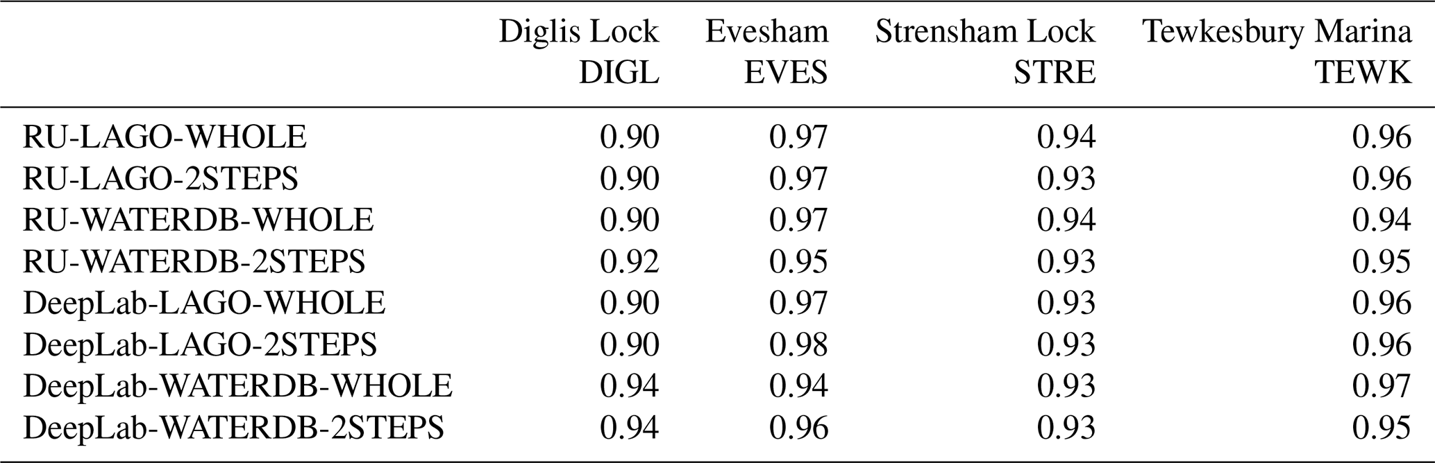
Figure 10 Standardised SOFI of the best window from the 4×4 grid in comparison with standardised water levels from nearby river gauges.

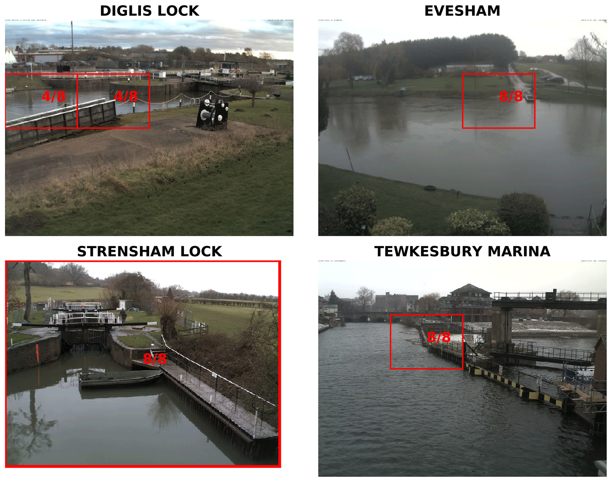
Figure 11 Windows of the 4×4 grid where the segmentation gives the best correlation with the water level for at least one of the eight networks considered. The fractions correspond to the proportion of networks that selected the corresponding window as the one giving the best correlation.

4 Conclusions

This work addressed the problem of water segmentation using river-camera images to automate the process of water-level estimation. We tackled the problem of water segmentation by applying transfer learning techniques to deep semantic segmentation networks trained on large datasets of natural images.

The first experiment regarding the classification of landmarks annotated with water-level information on small 2 week datasets showed that the best water segmentation networks were able to reach balanced accuracy greater than 91 % for each of the studied locations, which proved the good segmentation performance of our algorithm and showed its potential in the context of flood-extent analysis studies.

The landmark-based water-level estimation (LBWLE) algorithm was then developed for this work. It allows direct estimation of the water-level from the classified landmarks. The experiments performed with LBWLE showed that it was possible to estimate the water level with the maximum accuracy this algorithm could reach, as it is inherently limited by the heights of the landmarks used for the study. Given a camera location and a detailed ground survey in the field of view of the camera, this approach can, however, provide an accurate estimation of the water level, in absolute units, without any need for calibration at the camera location.

With the second experiment, much larger, year-long datasets of images with no water-level annotations available were created. This experiment used available water levels from nearby river gauges as validation data and showed that the water levels estimated using the LBWLE approach could also be used in this context. Indeed, the approach developed in this work was able to measure the water levels for the three major floods that happened during the year.

This second experiment also investigated the use of the static observer flooding index (SOFI) (Moy de Vitry et al., 2019) applied on the entire image to show that results obtained were strongly correlated with the water level from the nearby river gauges. This showed that it was possible to use the SOFI to track flood events and have a better tracking of lower flows while the river is still in-bank than when using LBWLE. However, for one location, occlusions occurring in the field of view of the camera impacted the results.

Finally, a simple approach that computes the SOFI on a specific window (sub-region) of the image was investigated during this second experiment. This window is selected through a simple validation procedure using older images and water levels from the same locations. This approach allowed accurate tracking of large flood events as well as smaller changes while the river is still in-bank on every dataset. While this approach is the most accurate that was developed during this study, the choice of the window relies on relatively close river gauges. However, some straightforward guidelines in order to help the potential user to chose the window if nearby gauges are not available were suggested.

The algorithms and experiments presented in this study show the great potential of transfer learning and semantic segmentation networks for the automation of the water-level estimations. These methods could drastically reduce the costs and workloads related to the evaluation of water levels, which is necessary for many applications, including the understanding of the ever increasing number of flood events.

Future work will focus on the merging of the water segmentation results with lidar digital surface model (DSM) data available at 1 m resolution over the UK (Environment Agency, 2017). This would allow the water segmentation algorithms to provide a direct estimate of the water levels in the areas that are studied without requiring any ground surveys.