Plant hydraulic transport controls transpiration sensitivity to soil water stress

Plant transpiration downregulation in the presence of soil water stress is a critical mechanism for predicting global water, carbon, and energy cycles. Currently, many terrestrial biosphere models (TBMs) represent this mechanism with an empirical correction function (β) of soil moisture – a convenient approach that can produce large prediction uncertainties. To reduce this uncertainty, TBMs have increasingly incorporated physically based plant hydraulic models (PHMs). However, PHMs introduce additional parameter uncertainty and computational demands. Therefore, understanding why and when PHM and β predictions diverge would usefully inform model selection within TBMs. Here, we use a minimalist PHM to demonstrate that coupling the effects of soil water stress and atmospheric moisture demand leads to a spectrum of transpiration responses controlled by soil–plant hydraulic transport (conductance). Within this transport-limitation spectrum, β emerges as an end-member scenario of PHMs with infinite conductance, completely decoupling the effects of soil water stress and atmospheric moisture demand on transpiration. As a result, PHM and β transpiration predictions diverge most for soil–plant systems with low hydraulic conductance (transport-limited) that experience high variation in atmospheric moisture demand and have moderate soil moisture supply for plants. We test these minimalist model results by using a land surface model at an AmeriFlux site. At this transport-limited site, a PHM downregulation scheme outperforms the β scheme due to its sensitivity to variations in atmospheric moisture demand. Based on this observation, we develop a new “dynamic β” that varies with atmospheric moisture demand – an approach that overcomes existing biases within β schemes and has potential to simplify existing PHM parameterization and implementation.

1 Introduction

Plants control their transpiration (T) and CO₂ assimilation by adjusting leaf stomatal apertures in response to environmental variations (Katul et al., 2012; Fatichi et al., 2016). In doing so, they mediate the global water, carbon, and energy cycles. The performance of most terrestrial biosphere models (TBMs) relies on accurately representing leaf stomatal responses in terms of stomatal conductance (g_s). Extensive research has established the relationships between g_s and atmospheric conditions like photosynthetically active radiation, humidity, CO₂ concentration, and air/leaf temperature under well-watered conditions, though the specific forms of these relationships vary (Damour et al., 2010; Buckley and Mott, 2013; Buckley, 2017). However, representing the dynamics of g_s in response to soil water stress remains problematic.

Many TBMs represent declining g_s and, in turn, transpiration reduction (i.e., downregulation) in response to soil water stress with an empirical function of soil water availability. This method, known as β (Powell et al., 2013; Verhoef and Egea, 2014; Trugman et al., 2018; Paschalis et al., 2020), reduces g_s from its peak value under well-watered conditions (g_s,ww), i.e., $g_{\mathrm{s}}=\mathit{\beta }\cdot g_{\mathrm{s},\mathrm{ww}}$, $\mathrm{0}\le \mathit{\beta }\le \mathrm{1}$. (We use the term “β” in this paper to refer to the downregulation model itself, and the terms “β function” and “β factor” to refer to the empirical function and its values, respectively.) The term “well-watered” refers to moist soil conditions where stomatal aperture is unaffected by plant water uptake from the soil, i.e., no soil water stress. The first β-like function appeared, to the best of our knowledge, in an early global heat balance study (Budyko, 1956) to reduce “evaporability” (comparable to well-watered g_s and T) for unsaturated land surfaces using a normalized soil moisture value. This method was eventually incorporated into the hydrology component of one of the first global circulation models (Manabe, 1969). However, many current β functions appear to stem from the heuristic root water uptake assumptions originally implemented in the crop transpiration model SWATR (Feddes et al., 1976, 1978), which evolved into the widely used SWAP model (Kroes et al., 2017). Since then, β has gained widespread use within TBMs and hydrological models due to its parsimonious form.

However, mounting evidence indicates that using β in TBMs is a major source of uncertainty and bias in plant-mediated carbon and water flux predictions. Multiple studies have implicated the lack of a universal β formulation as a primary source of inter-model variability in carbon cycle predictions (Medlyn et al., 2016; Rogers et al., 2017; Trugman et al., 2018; Paschalis et al., 2020). For example, different β formulations among nine TBMs accounted for 40 %–80 % of inter-model variability in global gross primary productivity (GPP) predictions (on the order of 3 %–286 % of current global GPP) (Trugman et al., 2018). Aside from the uncertainty in functional form, β appears to fundamentally misrepresent the coupled effects of soil water stress and atmospheric moisture demand on stomatal closure. Recent work using model–data fusion at FLUXNET sites highlighted that β produces stomatal responses that are overly sensitive to soil water stress and unrealistically insensitive to atmospheric moisture demand (Liu et al., 2020). Furthermore, TBM validation experiments have found that β schemes produce unrealistic GPP prediction during drought at Amazon rainforest sites (Powell et al., 2013; Restrepo-Coupe et al., 2017) and systematic overprediction of evaporative drought duration, magnitude, and intensity at several AmeriFlux sites (Ukkola et al., 2016). The apparent inadequacy of β has lead to the adoption of physically based plant hydraulic models (PHMs) in TBMs (Williams et al., 2001; Bonan et al., 2014; Xu et al., 2016; Kennedy et al., 2019; Eller et al., 2020; Sabot et al., 2020).

PHMs represent water transport, driven by a gradient of water potential energy, through the soil–plant–atmosphere continuum via flux-gradient relationships (based on Hagen–Poiseuille flow), which use measurable soil properties and plant traits as parameters (Mencuccini et al., 2019). The implementation of PHMs in several popular TBMs (e.g., CLM, JULES, etc.) has improved predictions in site-specific GPP and evapotranspiration (ET) predictions (Powell et al., 2013; Bonan et al., 2014; Kennedy et al., 2019; Eller et al., 2020; Sabot et al., 2020) as well as soil water dynamics (Kennedy et al., 2019) compared to β. PHMs also exhibit more realistic sensitivity to atmospheric moisture demand than β (Liu et al., 2020). However, these improvements from PHMs come at the cost of an increased number of plant hydraulic trait parameters and computational burden, which can reduce the reliability of the predictions (Prentice et al., 2015). Additionally, obtaining representative plant hydraulic trait values for a soil–plant system is difficult for two main reasons: (i) traits vary widely across and within species (Anderegg, 2015) and exhibit plasticity through acclimation and adaptation (Franks et al., 2014), and (ii) trait measurements are typically made at a single point (e.g., stem, branch, leaf), which may not reliably scale to represent whole-plant or ecosystem-level responses due to the effects of nonlinear trait variations along the soil–plant system (Couvreur et al., 2018). These difficulties result in uncertainty in the model predictions that may be further compounded at the ecosystem level (Fisher et al., 2018; Feng, 2020). Consequently, modelers continue to rely on β as a parsimonious alternative to PHMs (Paschalis et al., 2020).

The relative strengths and weaknesses of β and PHMs suggest that informed model selection requires a better understanding of when the complexity of a PHM is justified over the simplicity of β. This paper informs such understanding by (i) analyzing the fundamental differences between PHMs and β (Sect. 3.1), (ii) defining the parameters controlling the differences (Sect. 3.2), and (iii) demonstrating how PHMs outperform β for a real soil–plant system (Sect. 3.3). Then, leveraging our theoretical insights, we create a new “dynamic β” as a potential tool to correct the biases from the original β while reducing the parameter and computational demands of PHMs (Sect. 3.3). To accomplish these goals, we first analyze a minimalist PHM using a water supply–demand framework, then corroborate the results for a more widely used complex PHM, and, finally, perform a case study with a calibrated land surface model (LSM), which employs β, PHM, and dynamic β downregulation schemes.

2 Methods

2.1 Minimalist PHM

Our minimalist (Sect. 3.1–3.2) and complex PHM formulations (Sect. 3.3), illustrated in Fig. 1, rely on a supply–demand framework that conceptualizes transpiration as the joint outcome of soil water supply and atmospheric moisture demand (Gardner, 1960; Cowan, 1965; Sperry and Love, 2015; Kennedy et al., 2019). In this framework, “supply” refers to the rate of water transport to the leaf mesophyll cells from the soil, into the roots, and through the xylem. “Demand” refers to the rate of water vapor outflux through the stomata, driven by the transport capacity of the air surrounding the plant and regulated by the stomatal response to atmospheric conditions (Buckley, 2017) and leaf water status (Klein, 2014; Buckley, 2019). We assume steady-state transpiration fluxes (i.e., supply equals demand), which means we neglect the effects of plant capacitance (Bohrer et al., 2005) and also assume that the mean plant and atmospheric states equilibrate quickly over short timescales.

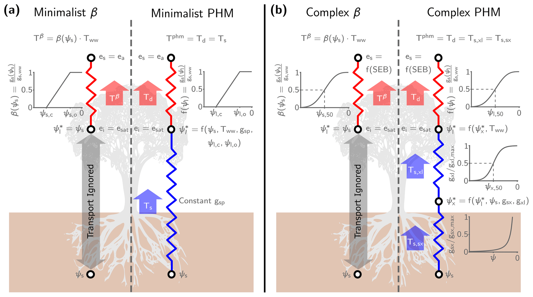
Figure 1 Schematic for the minimalist (a) and complex (b) β and PHM models used in this analysis. The resistors represent the conductance between soil–plant segments (i.e., an analogy to Ohm's law) that mediate liquid water supply (blue) and atmospheric water vapor demand (red). Next to each resistor is the segment-specific conductance downregulation curve dependent on water potential (ψ). The white circles indicate segment endpoints where we calculate the potentials (ψ) for liquid water transport and vapor pressures (e) for water vapor transport. The supply segment subscripts represent soil (s), xylem (x), leaf (l), and bulk soil-plant (sp), whereas the demand segment subscripts represent inside the leaf (i), at the leaf surface (s), and the ambient air (a). For water vapor transport, we assume saturation vapor pressure inside the leaf (e_i=e_sat) for both models. In the minimalist models, we assume the leaf surface vapor pressure (e_s) is the atmospheric vapor pressure (e_a), which makes the driving force for water vapor transport the leaf-to-air vapor pressure deficit ($D=e_{\mathrm{sat}}-e_{\mathrm{a}}$). Alternately, in the complex models, e_s is a function of the surface energy balance (f(SEB)) calculations at each time step. The thick arrows represent the water transport through each segment calculated by the integrated steady-state flux-gradient relationships discussed in Sect. 2.1–2.2 and 2.5. We use the minimalist models (left panel) for Sect. 3.1–3.2 and the complex models (right panel) for the LSM analysis in Sect. 3.3. (Note that we only illustrate a single big-leaf formulation here, but see Sect. S2 for the two-big-leaf implementation.)

The minimalist PHM supply (T_s [mm d⁻¹]; Eq. 1 and blue segment in Fig. 1a) is represented by a steady-state integrated 1-D flux-gradient relationship, bounded by the root-zone-average soil water potential (ψ_s [MPa]) and leaf water potential (ψ_l [MPa]) and mediated by the bulk conductance along the flow path (g_sp(ψ) $\left[\mathrm{mm}{\mathrm{d}}^{-\mathrm{1}}{\mathrm{MPa}}^{-\mathrm{1}}\right]$). For simplicity, we assume constant soil–plant conductance (g_sp) and ignore its dependence on water potential (i.e., hydraulic limits; Sperry et al., 1998). This assumption simplifies the integral in Eq. (1) to the product of g_sp and the water potential difference, ψ_s−ψ_l, which drives the flow.

$$\begin{array}{}\text{(1)}& T_{\mathrm{s}}=-\underset{{\mathit{\psi }}_{\mathrm{s}}}{\overset{{\mathit{\psi }}_{\mathrm{l}}}{\int }}{g}_{\mathrm{sp}}\left(\mathit{\psi }\right)d\mathit{\psi }=g_{\mathrm{sp}}\cdot \left({\mathit{\psi }}_{\mathrm{s}}-{\mathit{\psi }}_{\mathrm{l}}\right)\end{array}$$

The minimalist PHM demand (T_d [mm d⁻¹]; Eq. 2 and red segment in Fig. 1a) uses a similar conductance-difference formulation (i.e., integrated flux-gradient relationship). Transpiration is driven by the leaf-to-air water vapor pressure deficit (D [mol H₂O per mol air]) and mediated by the well-watered stomatal conductance (g_s,ww $\left[\mathrm{mol}\mathrm{air}{\mathrm{m}}^{-\mathrm{2}}{\mathrm{s}}^{-\mathrm{1}}\right]$), a stomatal closure term (f(ψ_l)), and the leaf area index (LAI [m² leaf m⁻² ground]). Additionally, we convert T_d from a molar flux to a volume flux using the conversion factor C_a (i.e., the molar weight of water (M_w [kg mol⁻¹]) divided by water density (ρ_w [kg m⁻³]) and multiplied by the conversion from m s⁻¹ to mm d⁻¹). The driving force D assumes saturation vapor pressure inside the leaf (i.e., e_i=e_sat) and that the leaf surface (e_s) and atmospheric vapor pressure (e_a) are the same (i.e., the leaf is well-coupled to the atmosphere; Jarvis and McNaughton, 1986); however, the leaf temperature can differ from the atmosphere, which differentiates D from atmospheric vapor pressure deficit (Grossiord et al., 2020). The parameter g_s,ww encapsulates the stomatal response to atmospheric conditions only (i.e., light, temperature, humidity, and CO₂ concentration). We define the product of LAI, g_s,ww, and D as the well-watered transpiration rate (T_ww) – which represents atmospheric moisture demand throughout this paper – and we specify its value for the minimalist analysis. The term “well-watered” refers to abundant soil water conditions under which water transport to the leaves maintains ψ_l high enough to avoid stomatal closure. During water-stressed conditions, the f(ψ_l) term represents stomatal closure (i.e., downregulating g_s,ww) to lowering leaf water status (Buckley, 2019). We assume a normalized, piecewise linear f(ψ_l) (Eq. 3 and illustrated in Fig. 1a), parametrized by the leaf water potential at incipient (ψ_l,o) and complete stomatal closure (ψ_l,c). This simple multiplicative reduction of g_s,ww (similar to the approach of Jarvis, 1976) captures the observed non-unique relationship between g_s and ψ_l (Anderegg and Venturas, 2020) while facilitating comparison with the similar minimalist β formulation (see Sect. 2.5).

$$\begin{array}{}\text{(2)}& {\displaystyle }{T}_{\mathrm{d}}=\mathrm{LAI}\cdot f\left({\mathit{\psi }}_{\mathrm{l}}\right)\cdot g_{\mathrm{s},\mathrm{ww}}\cdot D\cdot C_{\mathrm{a}}=f\left({\mathit{\psi }}_{\mathrm{l}}\right)\cdot T_{\mathrm{ww}}\cdot C_{\mathrm{a}};\text{(3)}& {\displaystyle }f\left({\mathit{\psi }}_{\mathrm{l}}\right)={\displaystyle \frac{g_{\mathrm{s}}\left({\mathit{\psi }}_{\mathrm{l}}\right)}{g_{\mathrm{s},\mathrm{ww}}}}=\left\{\begin{array}{ll}\mathrm{1}& {\mathit{\psi }}_{\mathrm{l}}\ge {\mathit{\psi }}_{\mathrm{l},\mathrm{o}},\\ \frac{{\mathit{\psi }}_{\mathrm{l},\mathrm{c}}-{\mathit{\psi }}_{\mathrm{l}}}{{\mathit{\psi }}_{\mathrm{l},\mathrm{c}}-{\mathit{\psi }}_{\mathrm{l},\mathrm{o}}}& {\mathit{\psi }}_{\mathrm{l},\mathrm{c}}<{\mathit{\psi }}_{\mathrm{l}}<{\mathit{\psi }}_{\mathrm{l},\mathrm{o}},\\ \mathrm{0}& {\mathit{\psi }}_{\mathrm{l}}\le {\mathit{\psi }}_{\mathrm{l},\mathrm{c}}.\end{array}\right.\end{array}$$

The PHM supply and demand are coupled through their mutual dependence on leaf water potential. The ψ_l value that balances supply (Eq. 1) and demand (Eq. 2) – which we will call ${\mathit{\psi }}_{\mathrm{l}}^{*}$ (Eq. 4) – yields the steady-state transpiration rate for the minimalist PHM (T^phm; Eq. 5). The full derivation of ${\mathit{\psi }}_{\mathrm{l}}^{*}$ and T^phm is shown in Sect. S1 in the Supplement.

$$\begin{array}{}\text{(4)}& {\displaystyle }{\mathit{\psi }}_{\mathrm{l}}^{*}={\displaystyle \frac{{\mathit{\psi }}_{\mathrm{s}}\cdot \left({\mathit{\psi }}_{\mathrm{l},\mathrm{o}}-{\mathit{\psi }}_{\mathrm{l},\mathrm{c}}\right)+\frac{T_{\mathrm{ww}}\cdot {\mathit{\psi }}_{\mathrm{l},\mathrm{c}}}{g_{\mathrm{sp}}}}{\left({\mathit{\psi }}_{\mathrm{l},\mathrm{o}}-{\mathit{\psi }}_{\mathrm{l},\mathrm{c}}\right)+\frac{T_{\mathrm{ww}}}{g_{\mathrm{sp}}}}};\text{(5)}& {\displaystyle }{T}^{\mathrm{phm}}=\left\{\begin{array}{ll}{T}_{\mathrm{ww}}& {\mathit{\psi }}_{\mathrm{s}}>{\mathit{\psi }}_{\mathrm{l},\mathrm{o}}+\frac{T_{\mathrm{ww}}}{g_{\mathrm{sp}}},\\ T_{\mathrm{ww}}\cdot \frac{\left({\mathit{\psi }}_{\mathrm{l},\mathrm{c}}-{\mathit{\psi }}_{\mathrm{s}}\right)}{\left({\mathit{\psi }}_{\mathrm{l},\mathrm{c}}-{\mathit{\psi }}_{\mathrm{l},\mathrm{o}}\right)-\frac{T_{\mathrm{ww}}}{g_{\mathrm{sp}}}}& {\mathit{\psi }}_{\mathrm{l},\mathrm{c}}<{\mathit{\psi }}_{\mathrm{s}}\le {\mathit{\psi }}_{\mathrm{l},\mathrm{o}}+\frac{T_{\mathrm{ww}}}{g_{\mathrm{sp}}},\\ \mathrm{0}& {\mathit{\psi }}_{\mathrm{s}}\le {\mathit{\psi }}_{\mathrm{l},\mathrm{c}}.\end{array}\right.\end{array}$$

2.2 Complex PHM

The LSM analysis (Sect. 3.3) uses a complex PHM formulation following Feng et al. (2018). The PHM separates supply into soil-to-xylem and xylem-to-leaf segments and demand into a leaf-to-atmosphere segment (Fig. 1b). Here, we briefly discuss the complex PHM components for a single big-leaf formulation; however, we refer the reader to Sects. S2–S3 for full model details and parameter values for the two-big-leaf formulation used in our LSM.

For PHM supply (T_s; blue segments in Fig. 1b), the water potential gradient drives flow through the soil–plant system mediated by the segment-specific conductances. Unlike the minimalist PHM (Sect. 2.1), we assume the conductance in each segment depends on water potential, which represents “hydraulic limits” (Sperry et al., 1998) that arise via (i) the inability of roots to remove water from soil pores at low ψ_s and (ii) xylem embolism caused by large hydraulic gradients required under low ψ_s and/or high T_ww. The soil-to-xylem conductance (g_sx $\left[\mathrm{mm}{\mathrm{d}}^{-\mathrm{1}}{\mathrm{MPa}}^{-\mathrm{1}}\right]$; Eq. 6 and illustrated in Fig. 1b) is its maximum value (g_sx,max) downregulated by the unsaturated soil hydraulic conductivity curve (Clapp and Hornberger, 1978), which is parametrized by the saturated soil water potential (ψ_sat), soil water retention exponent (b), unsaturated hydraulic conductivity exponent ($c=\mathrm{2}b+\mathrm{3}$), and a correction factor (d) to account for roots' ability to reach water (Daly et al., 2004). The xylem-to-leaf conductance (g_xl $\left[\mathrm{mm}{\mathrm{d}}^{-\mathrm{1}}{\mathrm{MPa}}^{-\mathrm{1}}\right]$; Eq. 7 and illustrated in Fig. 1b) is its maximum value (g_xl,max) downregulated by a sigmoidal function (Pammenter and Willigen, 1998), which is parametrized by the vulnerability exponent (a) and the xylem water potential (ψ_x) at 50 % loss of conductance (ψ_x,50). We estimate the maximum conductance values for each segment (g_sx,max and g_xl,max) with trait-based equations following Feng et al. (2018) (see Sect. S2.5.3). Given that conductance varies with water potential, we utilize a Kirchhoff transform (Eq. 8) to approximate the water supply from each segment (T_s,sx and T_s,xl [mm d⁻¹]; Eqs. 9–10) as the difference in the matric flux potential (Φ [mm d⁻¹]) at the segment endpoints. Therefore, given a value of ψ_s (i.e., root-zone-average water potential) and ψ_l, the ψ_x that balances T_s,sx and T_s,xl – called ${\mathit{\psi }}_{\mathrm{x}}^{*}$ – yields the steady-state supply rate (T_s).

$$\begin{array}{}\text{(6)}& g_{\mathrm{sx}}\left(\mathit{\psi }\right)=g_{\mathrm{sx},\max }\cdot {\left({\displaystyle \frac{{\mathit{\psi }}_{\mathrm{sat}}}{\mathit{\psi }}}\right)}^{\frac{c-d}{b}},\end{array}$$

$$\begin{array}{}\text{(7)}& {\displaystyle }{g}_{\mathrm{xl}}\left(\mathit{\psi }\right)=g_{\mathrm{xl},\max }\cdot \left[\mathrm{1}-{\displaystyle \frac{\mathrm{1}}{\mathrm{1}+e^{a\cdot \left(\mathit{\psi }-{\mathit{\psi }}_{\mathrm{x},\mathrm{50}}\right)}}}\right],\text{(8)}& {\displaystyle }\mathrm{\Phi }\left(\mathit{\psi }\right)=\underset{-\mathrm{\infty }}{\overset{\mathit{\psi }}{\int }}g\left({\mathit{\psi }}^{\prime }\right)d{\mathit{\psi }}^{\prime },\text{(9)}& {\displaystyle }{T}_{\mathrm{s},\mathrm{sx}}={\mathrm{\Phi }}_{\mathrm{sx}}\left({\mathit{\psi }}_{\mathrm{s}}\right)-{\mathrm{\Phi }}_{\mathrm{sx}}\left({\mathit{\psi }}_x\right),\text{(10)}& {\displaystyle }{T}_{\mathrm{s},\mathrm{xl}}={\mathrm{\Phi }}_{\mathrm{xl}}\left({\mathit{\psi }}_x\right)-{\mathrm{\Phi }}_{\mathrm{xl}}\left({\mathit{\psi }}_{\mathrm{l}}\right).\end{array}$$

The complex PHM demand (T_d [mm d⁻¹]; Eq. 11 and red segment in Fig. 1b) mirrors the minimalist version (Eq. 2) with modifications to fit into a dual-source LSM scheme (Sect. 2.3) that explicitly represents the coupled mass, heat and energy transfer between the plant, its microclimate, and the atmosphere. The driving force of transpiration is no longer D (i.e., the leaf-to-air vapor pressure deficit) but rather the difference between leaf internal (e_i [kPa]) and surface (e_s [kPa]) vapor pressure (normalized by atmospheric pressure (P_atm [kPa]) to obtain units mol H₂O per mol air). We still assume e_i is the saturation vapor pressure at leaf temperature (e_sat), but now e_s depends on the plant microclimate determined by the LSM energy balance solution at each time step (see Sect. S2.6). This plant microclimate is coupled to the well-watered stomatal conductance (g_s,ww $\left[\mathrm{mol}\mathrm{air}{\mathrm{m}}^{-\mathrm{2}}{\mathrm{s}}^{-\mathrm{1}}\right]$) via the optimality-based stomatal response model of Medlyn et al. (2011). The Medlyn model (Eq. 12) depends on the leaf vapor pressure difference (e_i−e_s [kPa]), net CO₂ assimilation rate (A_n $\left[\mathrm{mol}{\mathrm{CO}}_{\mathrm{2}}{\mathrm{m}}^{-\mathrm{2}}{\mathrm{s}}^{-\mathrm{1}}\right]$), and the leaf surface CO₂ mole fraction (approximated by the ratio of leaf surface CO₂ partial pressure (c_s [kPa]) and P_atm to give units mol CO₂ per mol air) and is parametrized by the minimum stomatal conductance (g_o $\left[\mathrm{mol}\mathrm{air}{\mathrm{m}}^{-\mathrm{2}}{\mathrm{s}}^{-\mathrm{1}}\right]$) and a slope parameter (g₁ [kPa^0.5]). Furthermore, we couple g_s,ww to the Farquhar et al. (1980) photosynthesis model through A_n to ensure CO₂ diffusion into the leaf balances carbon assimilation (Collatz et al., 1991) (see Sect. S2.4). As in the minimalist model, the product of g_s,ww, driving force, and LAI yields the well-watered transpiration rate, T_ww, which we take to represent atmospheric moisture demand. Under water-stressed conditions, we keep a Jarvis-like stomatal closure term (f(ψ_l)) to downregulate g_s,ww, because it facilitates easy comparisons between our minimalist and complex formulations. However, we upgrade f(ψ_l) from a piecewise linear form (Eq. 3) to a more realistic Weibull form (Eq. 13 and illustrated in Fig. 1b) parametrized by a shape factor describing stomatal sensitivity (b_l) and the leaf water potential at 50 % loss of stomatal conductance (ψ_l,50 [MPa]) (Klein, 2014; Kennedy et al., 2019).

$$\begin{array}{}\text{(11)}& {\displaystyle }{T}_{\mathrm{d}}=\mathrm{LAI}\cdot f\left({\mathit{\psi }}_{\mathrm{l}}\right)\cdot g_{\mathrm{s},\mathrm{ww}}\cdot {\displaystyle \frac{e_{\mathrm{i}}-e_{\mathrm{s}}}{P_{\mathrm{atm}}}}\cdot C_{\mathrm{a}}=f\left({\mathit{\psi }}_{\mathrm{l}}\right)\cdot T_{\mathrm{ww}}\cdot C_{\mathrm{a}},\text{(12)}& {\displaystyle }{g}_{\mathrm{s},\mathrm{ww}}=g_{\mathrm{o}}+\left(\mathrm{1}+{\displaystyle \frac{g_{\mathrm{1}}}{\sqrt{e_{\mathrm{i}}-e_{\mathrm{s}}}}}\right)\cdot {\displaystyle \frac{\mathrm{1.6}\cdot A_{\mathrm{n}}}{c_{\mathrm{s}}/P_{\mathrm{atm}}}},\text{(13)}& {\displaystyle }f\left({\mathit{\psi }}_{\mathrm{l}}\right)={\displaystyle \frac{g_{\mathrm{s}}\left({\mathit{\psi }}_{\mathrm{l}}\right)}{g_{\mathrm{s},\mathrm{ww}}}}={\mathrm{2}}^{-{\left(\frac{{\mathit{\psi }}_{\mathrm{l}}}{{\mathit{\psi }}_{\mathrm{l},\mathrm{50}}}\right)}^{b_{\mathrm{l}}}}.\end{array}$$

As in the minimalist PHM, the complex PHM supply and demand are coupled through their mutual dependence on ψ_l. The ${\mathit{\psi }}_{\mathrm{l}}^{*}$ that balances T_s (found at ${\mathit{\psi }}_{\mathrm{x}}^{*}$ for Eqs. 9–10) and T_d (Eq. 11) yields the steady-state transpiration rate for the complex PHM (T^phm). We numerically calculate this solution by recasting Eqs. (9)–(11) as a nonlinear least squares problem and finding the ${\mathit{\psi }}_{\mathrm{l}}^{*}$ and ${\mathit{\psi }}_x^{*}$ that ensure mass balance between the segments (see Sect. S2.5.3).

2.3 LSM description and calibration

We created an LSM to test several transpiration downregulation schemes (Sect. 3.3) and allow for removal of modules (e.g., subsurface heat and mass transfer) that would unnecessarily complicate our comparisons. Our LSM is a dual-source two-big-leaf approximation (Bonan, 2019) adapted from CLM v5 (Oleson et al., 2018) with several key simplifications: (i) steady-state conditions (i.e., no aboveground mass, heat, or energy storage), (ii) neutral atmospheric stability, (iii) implemented the Goudriaan and van Laar (1994) radiative transfer model in lieu of the two-stream approximation (Oleson et al., 2018), and (iv) forced the LSM with soil moisture, soil heat flux, and downwelling radiation data. We refer the reader to Sect. S2 for full model details and justifications. We formulated the LSM in MATLAB and have made our codes available online (Sloan, 2021; https://doi.org/10.5281/zenodo.5129247).

We created separate LSM versions to test five different transpiration downregulation schemes: (i) well-watered (no downregulation), (ii) a single β (β_s) with static parameters, (iii) a β separately applied to sunlit and shaded leaf areas (β_2L) with static parameters, (iv) a dynamic β with parameters dependent on T_ww (β_dyn), and (v) a PHM. We calibrated the PHM version using a two-step approach. First, we simulated 13 600 parameter sets using Progressive Latin Hypercube Sampling (Razavi et al., 2019) on 15 soil and plant parameters (Table S6) and selected the best parameter set based on a comparison of RMSE, correlation coefficient, percent bias, and variance to AmeriFlux evapotranspiration, sensible heat flux, gross primary productivity, and net radiation site data (Figs. S5–S8). Unfortunately, the best parameter set contained an unrealistically low ψ_l,50 value for ponderosa pine compared to observations (DeLucia and Heckathorn, 1989). Therefore, as a second step, we adjusted the ψ_l,50 and several other soil and plant parameters to more realistic values while ensuring that they replicated the transpiration downregulation behavior of the original parameter set. These parameter adjustments had minimal impact on the LSM predictions as the underlying equations are highly nonlinear, and multiple parameter sets can give near equivalent results (i.e., equifinality). We refer the reader to Sect. S4 for a more detailed account of calibration.

We parametrized the three LSM versions containing the β schemes by calibrating the respective β functions to the relative transpiration outputs ($T/T_{\mathrm{ww}}$) of the calibrated PHM version, while we ran the well-watered version using the calibrated parameters and downregulation turned off. The choice to calibrate a single LSM version ensured that the performance differences between the schemes would be due to the PHM representing plant water use more realistically and not to the artifact of differing parameter fits between LSM versions. We refer the reader to Sect. S6.2 for specific details of the parameter fits for the β schemes.

2.4 Site description and forcing data

We calibrated and forced the LSM with half-hourly data from the US-Me2 “Metolius” AmeriFlux site (Irvine et al., 2008) for daylight hours during May-August 2013-2014. The forcing data were taken from both the AmeriFlux (Law, 2021) and FLUXNET2015 (FLUXNET2015, 2019; Pastorello et al., 2020) data products (see Sect. S5 for full details). The site consists of intermediate-age ponderosa pine trees on sandy loam soil in the Metolius River basin in Oregon, USA. We selected this site specifically for its subsurface soil moisture and temperature profiles as well as its separate measurements of photosynthetically active radiation (PAR) and near-infrared radiation (NIR). We used these boundary condition data to force the LSM in lieu of solving one-dimensional subsurface mass and heat transfer equations and atmospheric radiation partitioning models. In particular, we forced the LSM with root-zone-averaged soil water potential (ψ_s; estimated from measured soil water content and a pedotransfer function) and the ground heat flux measurements. We selected the measurement depth of 50 cm to represent ψ_s based on the deviation of measured GPP from its mean in relation to measured soil water content and vapor pressure deficit (Fig. S10). The 50 cm measurements showed clear GPP downregulation under water stress. Furthermore, the depth seemed reasonable given previous modeling at this site estimated an effective rooting depth of 1.1 m (Schwarz et al., 2004). The atmospheric forcing for the LSM consisted of incoming direct and diffuse NIR and PAR fluxes, CO₂ concentration, atmospheric pressure, vapor pressure, temperature, and wind velocity at the measurement tower height of 32 m. Full description of the forcing data is given in Sect. S5.

2.5 β formulations

The β function empirically represents stomatal closure to declining leaf water status caused by soil water stress. By design, β makes the simplifying assumption that stomata respond directly to soil water status (to avoid the complexity of implementing a PHM as illustrated by Fig. 1), which is readily available in TBM subsurface hydrology schemes as ψ_s or volumetric soil water content (θ_s). This heuristic approach leads to multiple β functions based on modeler preference (see the supplement of Trugman et al., 2018, for a list of differing β formulations common to TBMs). Furthermore, even if a universal β function existed, there is open debate on how to apply the β factor (Egea et al., 2011); some TBMs apply the β factor directly to stomatal conductance (Kowalczyk et al., 2006; De Kauwe et al., 2015; Wolf et al., 2016), whereas others indirectly affect stomatal conductance by applying the β factor to photosynthetic parameters (Zhou et al., 2013; Lin et al., 2018; Kennedy et al., 2019). Here, we select a single β formulation that easily compares with the demand component of our PHM. Selecting a different β formulation could alter our values; however, we do not expect our main conclusions about β and PHM differences to change as long as two criteria are met. First, the stomatal downregulation factors for the PHM (f(ψ_l)) and β (β(ψ_s)) are applied consistently in the transpiration downregulation scheme (to either g_s,ww or photosynthetic parameters). Second, if β is in terms of θ_s, a curvilinear form must be used (Egea et al., 2011) to ensure β can be mapped approximately to the water potential space of our analysis.

In this paper, we have defined the β function in terms of ψ_s and apply the β factor directly to g_s,ww and, in turn, T_ww (Eq. 14) for three key reasons: (i) water transport through the soil–plant–atmosphere continuum follows a gradient of water potential, not water content, (ii) β using ψ_s rather than θ_s produces more realistic downregulation behavior compared to data (Verhoef and Egea, 2014), and (iii) applying the β factor to g_s,ww directly corresponds to the PHM demand in both minimalist and complex formulations. In the minimalist analysis (Sect. 3.1–3.2), β(ψ_s) (Eq. 15 and illustrated in Fig. 1a) takes a piecewise linear form (analogous to Eq. 3), which is parametrized by the soil water potential at incipient (ψ_s,o) and complete stomatal closure (ψ_s,c). Similarly, in the LSM analysis (Sect. 3.3), β(ψ_s) (Eq. 16 and illustrated in Fig. 1b) takes a Weibull form (analogous to Eq. 13) parametrized by the soil water potential at 50 % loss of stomatal conductance (ψ_s,50) and a stomatal sensitivity parameter (b_s). The LSM analysis uses two versions of Eq. 16: (i) a static version with constant b_s and ψ_s,50 (used by the β_s and β_2L schemes) and (ii) a dynamic version where b_s and ψ_s,50 are linear functions of T_ww (used by the β_dyn scheme). We refer the reader to Fig. S12 for illustrations of the different β versions.

$$\begin{array}{}\text{(14)}& {\displaystyle }{T}^{\mathit{\beta }}=\mathit{\beta }\left({\mathit{\psi }}_{\mathrm{s}}\right)\cdot T_{\mathrm{ww}};\text{(15)}& {\displaystyle }\mathit{\beta }\left({\mathit{\psi }}_{\mathrm{s}}\right)=\left\{\begin{array}{ll}\mathrm{1}& {\mathit{\psi }}_{\mathrm{s}}\ge {\mathit{\psi }}_{\mathrm{s},\mathrm{o}},\\ \frac{{\mathit{\psi }}_{\mathrm{s},\mathrm{c}}-{\mathit{\psi }}_{\mathrm{s}}}{{\mathit{\psi }}_{\mathrm{s},\mathrm{c}}-{\mathit{\psi }}_{\mathrm{s},\mathrm{o}}}& {\mathit{\psi }}_{\mathrm{s},\mathrm{c}}<{\mathit{\psi }}_{\mathrm{s}}<{\mathit{\psi }}_{\mathrm{s},\mathrm{o}},\\ \mathrm{0}& {\mathit{\psi }}_{\mathrm{s}}\le {\mathit{\psi }}_{\mathrm{s},\mathrm{c}};\end{array}\right.\text{(16)}& {\displaystyle }\mathit{\beta }({\mathit{\psi }}_{\mathrm{s}},T_{\mathrm{ww}})={\mathrm{2}}^{-{\left(\frac{{\mathit{\psi }}_{\mathrm{s}}}{{\mathit{\psi }}_{\mathrm{s},\mathrm{50}}\left(T_{\mathrm{ww}}\right)}\right)}^{b_{\mathrm{s}}\left(T_{\mathrm{ww}}\right)}}.\end{array}$$

3 Results

3.1 β as a limiting case of PHMs with infinite conductance

The supply–demand framework reveals that the minimalist PHM and β fundamentally differ in their coupling of the effects of soil water stress (represented by ψ_s) and atmospheric moisture demand (represented by T_ww) on transpiration. The PHM supply lines (red lines in Fig. 2a) illustrate soil-to-leaf water transport (Eq. 1) at a fixed soil water availability (ψ_s) under increasing pull from the leaf (lower ψ_l) and constant soil–plant conductance (g_sp; supply line slope). The PHM demand lines (black lines in Fig. 2a) illustrate transpiration reduction under lower ψ_l (from stomatal closure) for two T_ww values. The supply and demand lines intersect at the minimalist PHM solution (${\mathit{\psi }}_{\mathrm{l}}^{*}$ and T^phm; Eqs. 4–5). Therefore, the minimalist PHM couples the effects of soil water stress to atmospheric moisture demand on transpiration downregulation, because leaf water potential responds to ψ_s and T_ww until it reaches the point of steady-state transpiration (i.e., $T^{\mathrm{phm}}\left({\mathit{\psi }}_{\mathrm{l}}^{*}\right)=T_{\mathrm{s}}\left({\mathit{\psi }}_{\mathrm{l}}^{*}\right)=T_{\mathrm{d}}\left({\mathit{\psi }}_{\mathrm{l}}^{*}\right)$).

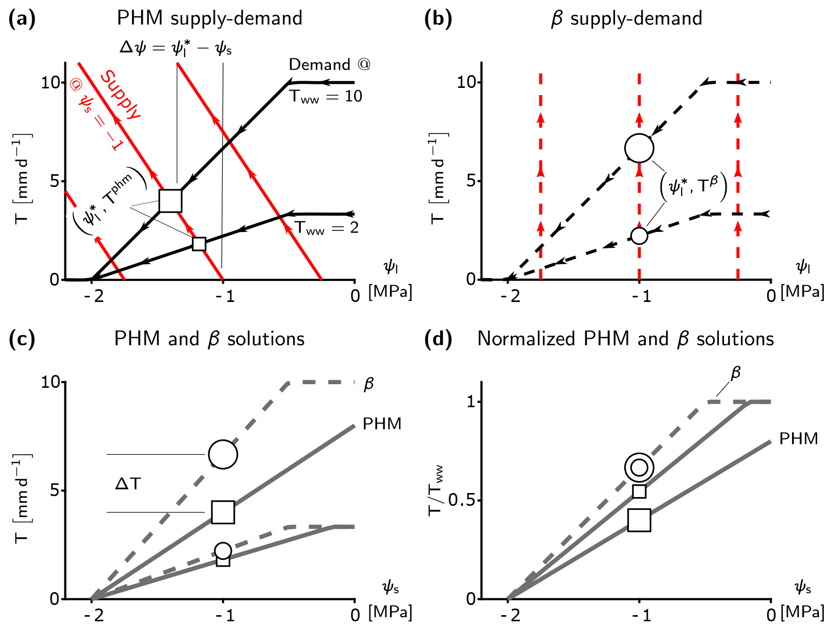
Figure 2 Fundamental differences between minimalist PHM and β. (a–b), Supply (red) and demand (black) curves for PHM (a, solid lines) and β (b, dashed lines) under varying leaf water potentials (ψ_l). The squares (circles) represent the PHM (β) solution – i.e., the ${\mathit{\psi }}_{\mathrm{l}}^{*}$ where supply equals demand – for a single soil water availability (ψ_s) and two atmospheric moisture demands (T_ww). These markers carry through panels (c) and (d) to illustrate how the solutions between the PHM and β diverge at a single ψ_s. The relative size of the markers indicates corresponding T_ww. The water potential difference Δψ required to transport water from soil to leaf is shown in panel (a) for ${\mathit{\psi }}_{\mathrm{s}}=-\mathrm{1}$ MPa and T_ww=10 mm d⁻¹. (c) Solutions of panels (a) and (b) mapped to ψ_s, where ΔT is the difference between PHM and β transpiration estimates at ${\mathit{\psi }}_{\mathrm{s}}=-\mathrm{1}$ MPa and T_ww=10 mm d⁻¹. (d) Relative transpiration, in which solutions in panel (c) are normalized by T_ww. The β solutions collapse to a single curve, whereas the PHM solutions depend on T_ww.

The minimalist β transpiration rate (T^β; Eq. 14) ignores this coupling as the β function depends only on ψ_s and independently reduces T_ww (shown in Fig. 1). The conditions leading to the decoupling in β only arise if the supply lines are vertical (Fig. 2b), which results in the relative transpiration ($T^{\mathit{\beta }}/T_{\mathrm{ww}}$) depending on ψ_s only (single curve in Fig. 2d). Since g_sp is the supply line slope (Eq. 1), β represents a limiting case of the PHM in which the soil–plant system is infinitely conductive. More specifically, as g_sp increases, the leaf water potential approaches the soil water potential (${\mathit{\psi }}_{\mathrm{l}}^{*}\to {\mathit{\psi }}_{\mathrm{s}}$; Eq. 17) and the PHM transpiration rate approaches the β transpiration rate (T^phm→T^β; Eq. 18). Therefore, the β(ψ_s) function (Eq. 15) equals the f(ψ_l) function (Eq. 3) in PHMs and represents stomatal closure to declining leaf (or soil) water potential. In summary, the empirical β physically represents an infinitely conductive soil–plant system where stomata close in response to leaf water potential that depends solely on the soil water potential with which it is equilibrated.

$$\begin{array}{}\text{(17)}& \underset{g_{\mathrm{sp}}\to \mathrm{\infty }}{lim}\left({\mathit{\psi }}_{\mathrm{l}}^{*}\right)=\underset{g_{\mathrm{sp}}\to \mathrm{\infty }}{lim}\left({\displaystyle \frac{{\mathit{\psi }}_{\mathrm{s}}\cdot \left({\mathit{\psi }}_{\mathrm{l},\mathrm{o}}-{\mathit{\psi }}_{\mathrm{l},\mathrm{c}}\right)+\frac{T_{\mathrm{ww}}\cdot {\mathit{\psi }}_{\mathrm{l},\mathrm{c}}}{g_{\mathrm{sp}}}}{\left({\mathit{\psi }}_{\mathrm{l},\mathrm{o}}-{\mathit{\psi }}_{\mathrm{l},\mathrm{c}}\right)+\frac{T_{\mathrm{ww}}}{g_{\mathrm{sp}}}}}\right)={\mathit{\psi }}_{\mathrm{s}}\end{array}$$

$$\begin{array}{}\text{(18)}& {\displaystyle }\begin{array}{rl}& \underset{g_{\mathrm{sp}}\to \mathrm{\infty }}{lim}\left(\mathrm{\Delta }T\right)=\underset{g_{\mathrm{sp}}\to \mathrm{\infty }}{lim}\left(T^{\mathrm{phm}}-T^{\mathit{\beta }}\right)=\underset{g_{\mathrm{sp}}\to \mathrm{\infty }}{lim}\\ & \left(T_{\mathrm{ww}}\cdot \left[{\displaystyle \frac{\left({\mathit{\psi }}_{\mathrm{l},\mathrm{c}}-{\mathit{\psi }}_{\mathrm{s}}\right)}{\left({\mathit{\psi }}_{\mathrm{l},\mathrm{c}}-{\mathit{\psi }}_{\mathrm{l},\mathrm{o}}\right)-\frac{T_{\mathrm{ww}}}{g_{\mathrm{sp}}}}}-{\displaystyle \frac{\left({\mathit{\psi }}_{\mathrm{l},\mathrm{c}}-{\mathit{\psi }}_{\mathrm{s}}\right)}{\left({\mathit{\psi }}_{\mathrm{l},\mathrm{c}}-{\mathit{\psi }}_{\mathrm{l},\mathrm{o}}\right)}}\right]\right)=\mathrm{0}.\end{array}\end{array}$$

The PHM coupling results in greater transpiration downregulation compared to β under the same environmental conditions (Fig. 2c). For a given soil water stress (ψ_s), β assumes ${\mathit{\psi }}_{\mathrm{s}}={\mathit{\psi }}_{\mathrm{l}}^{*}$ and downregulates any atmospheric moisture demand (T_ww) value by a fixed proportion (i.e., it scales linearly with T_ww); hence, it can be modeled with a single curve (Fig. 2d). Conversely, the PHM (with finite conductance) requires a water potential difference ($\mathrm{\Delta }\mathit{\psi }={\mathit{\psi }}_{\mathrm{s}}-{\mathit{\psi }}_{\mathrm{l}}^{*}$) to transport water from soil to leaf; therefore, ${\mathit{\psi }}_{\mathrm{l}}^{*}$ must be less than ψ_s, and greater stomatal closure results (Fig. 2c). Furthermore, the PHM downregulates transpiration at a greater proportion with increasing T_ww (i.e., it scales nonlinearly with T_ww) as it requires a greater Δψ and lower ${\mathit{\psi }}_{\mathrm{l}}^{*}$ (Fig. 2d). Hence, PHMs require transpiration downregulation to be described as a function of both ψ_s and T_ww.

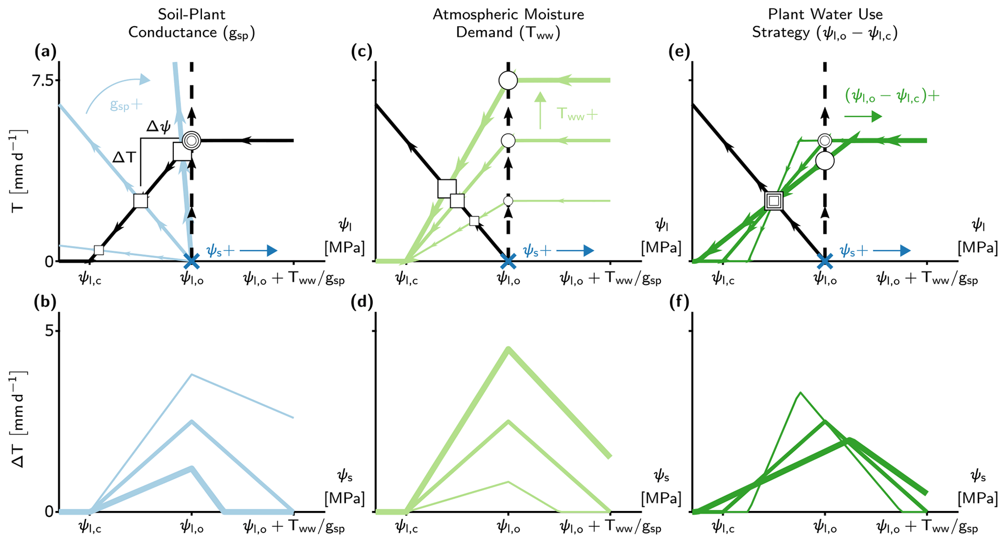
Figure 3 The effect of soil water potential (ψ_s), soil–plant conductance (g_sp), atmospheric moisture demand (T_ww), and plant water use strategy (${\mathit{\psi }}_{\mathrm{l},\mathrm{o}}-{\mathit{\psi }}_{\mathrm{l},\mathrm{c}}$) on differences between the minimalist PHM and β models (ΔT). (a, c, e) Supply–demand curves at a single soil water availability (indicated by the dark blue x at ${\mathit{\psi }}_{\mathrm{s}}={\mathit{\psi }}_{\mathrm{l},\mathrm{o}}$) for three prescribed values of g_sp, T_ww, and ${\mathit{\psi }}_{\mathrm{l},\mathrm{o}}-{\mathit{\psi }}_{\mathrm{l},\mathrm{c}}$, respectively. Each parameter (g_sp, T_ww, or ${\mathit{\psi }}_{\mathrm{l},\mathrm{o}}-{\mathit{\psi }}_{\mathrm{l},\mathrm{c}}$) is set at 50 % above (below) its base values at $g_{\mathrm{sp}}=\mathrm{10}\mathrm{mm}{\mathrm{d}}^{-\mathrm{1}}{\mathrm{MPa}}^{-\mathrm{1}}$, $T_{\mathrm{ww}}=\mathrm{5}\mathrm{mm}{\mathrm{d}}^{-\mathrm{1}}$, ${\mathit{\psi }}_{\mathrm{l},\mathrm{o}}=-\mathrm{1}\mathrm{MPa}$, and ${\mathit{\psi }}_{\mathrm{l},\mathrm{c}}=-\mathrm{2}\mathrm{MPa}$ using thick (thin) colored lines. The squares (circles) indicate the PHM (β) solutions, with size corresponding to magnitude of the changing parameter values. Note that the vertical distance between a correspondingly sized circle and square is ΔT, and horizontal distance is Δψ. (b, d, f) The ΔT results from panels (a), (c), and (e) calculated for a range of ψ_s with line thickness proportional to parameters in the aforementioned panels (e.g., thick blue line in panel b corresponds to 50 % increase in g_sp shown in panel a). The x axes are mapped from ψ_l in the top panels to ψ_s in the bottom panels.

These minimalist model results suggest that the range of soil–plant conductances (g_sp) can generate a spectrum of possible transpiration responses to soil water stress (and atmospheric moisture demand). Two classes of behaviors emerge – one in a “soil-limited” soil–plant system, in which g_sp is large enough for ψ_l≈ψ_s, thus decoupling the effects of soil water stress and atmospheric moisture demand while allowing the relative transpiration to vary only with ψ_s (Fig. 2d). The other class of behavior arises in “transport-limited” systems with finite g_sp, in which a non-negligible water potential difference (Δψ) is required to transport the water to the leaf, resulting in additional downregulation compared to soil-limited systems (Fig. 2c) and requiring relative transpiration to depend on both ψ_s and T_ww (Fig. 2d).

3.2 Parameters controlling the divergence of β and PHMs

The differences in PHM and β transpiration estimates (ΔT) depend not only on g_sp but also on soil water availability (ψ_s), atmospheric moisture demand (T_ww), and plant water use strategy (${\mathit{\psi }}_{\mathrm{l},\mathrm{o}}-{\mathit{\psi }}_{\mathrm{l},\mathrm{c}}$). To disentangle these joint dependencies, we adjust a single variable and explore the impact on ΔT using the supply and demand lines (Fig. 3). The translation of supply lines represents ψ_s changes (indicated in Fig. 3a, c, e) and produces a non-monotonic relationship with ΔT over the range of soil water stress (i.e., ${\mathit{\psi }}_{\mathrm{l},\mathrm{c}}<{\mathit{\psi }}_{\mathrm{s}}<{\mathit{\psi }}_{\mathrm{l},\mathrm{o}}+T_{\mathrm{ww}}/g_{\mathrm{sp}}$) (Fig. 3b, d, f). The peak ΔT occurs at the incipient point of stomatal closure (ψ_l,o) as (i) when ${\mathit{\psi }}_{\mathrm{s}}<{\mathit{\psi }}_{\mathrm{l},\mathrm{o}}$, transpiration begins to decrease, and in its extreme limit, transpiration (and thus ΔT) approaches 0, and (ii) when ${\mathit{\psi }}_{\mathrm{s}}>{\mathit{\psi }}_{\mathrm{l},\mathrm{o}}$, the effects of downregulation diminish in both models as the soil becomes well-watered. The ΔT–ψ_s behavior acts as a baseline relationship in the following analysis of g_sp, T_ww, and ${\mathit{\psi }}_{\mathrm{l},\mathrm{o}}-{\mathit{\psi }}_{\mathrm{l},\mathrm{c}}$ controls.

The ΔT–ψ_s relationship increases with lower g_sp (Fig. 3b; greater transport limitation) because flatter supply lines increase Δψ (Fig. 3a), requiring greater stomatal closure and hence additional downregulation for a PHM compared to β. Similarly, higher T_ww increases the ΔT–ψ_s relationship (Fig. 3d), although the increase in Δψ stems from steeper demand line slope (Fig. 3c). In addition to increasing ΔT at each ψ_s value, the effects of g_sp and T_ww increase the range of soil water stress above ψ_l,o (up to saturated soil water potential). This result indicates that PHMs can simulate transpiration downregulation under moist soil conditions that β potentially misses as it does not account for large Δψ values from transport limitation and/or high atmospheric moisture demand. Finally, as g_sp increases (soil-limited) and T_ww decreases, ΔT tends to zero, once again, for slightly different reasons: for g_sp, the supply lines approach the β assumption (vertical dashed line in Fig. 3a), whereas for T_ww, transpiration approaches zero.

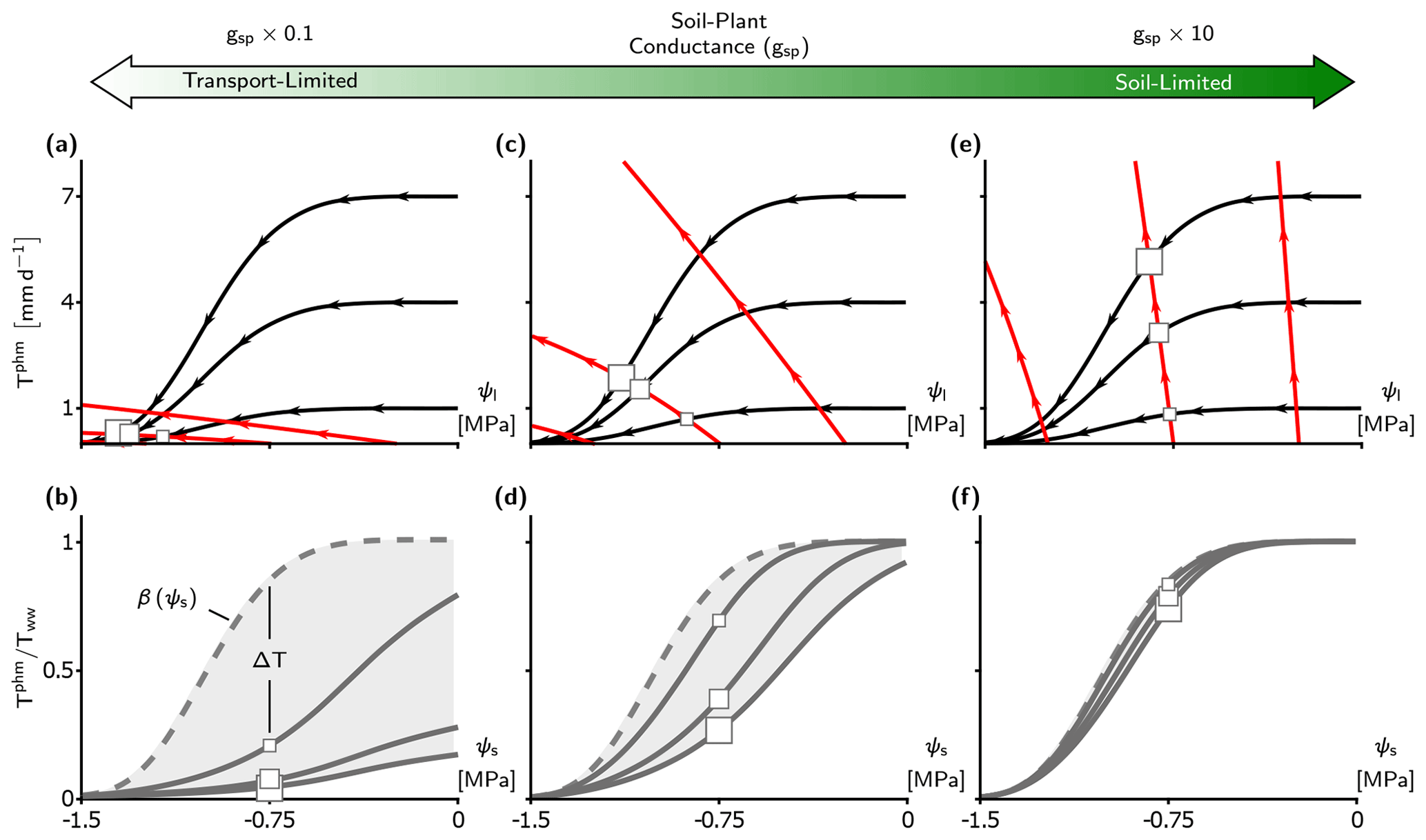
Figure 4 Transport-limitation spectrum observed in the complex PHM formulation. (a, c, e) Supply–demand curves for three values of soil–plant conductance, g_sp, using the complex PHM formulation. Panel (c) uses the calibrated LSM parameters from the US-Me2 AmeriFlux site discussed in Sect. 2.3. Panels (a) and (e) contain the calibrated conductance ($g_{\mathrm{sp}}\approx \mathrm{13}\mathrm{mm}{\mathrm{d}}^{-\mathrm{1}}{\mathrm{MPa}}^{-\mathrm{1}}$) multiplied by 0.1 and 10, respectively. The supply lines (red) are shown at ψ_s equal to 0, −0.75, and −1.5 MPa, and demand lines (black) are shown at T_ww equal to 1, 4, and 7 mm d⁻¹. The PHM solution for ψ_s at −0.75 MPa is shown by the squares with size corresponding to T_ww magnitude. (b, d, f) The relative transpiration for the PHM (solid) in panels (a), (c), and (e) and the infinitely conductive β solution (dashed line) are shown. The light gray shading indicates the PHM downregulation envelope bounded by β(ψ_s) as T_ww approaches zero and the relative transpiration curve at the highest T_ww.

Lastly, we explore the effect of plant water use strategy (${\mathit{\psi }}_{\mathrm{l},\mathrm{o}}-{\mathit{\psi }}_{\mathrm{l},\mathrm{c}}$) on ΔT – which approximates the sensitivity of stomatal closure to ψ_l. Altering ${\mathit{\psi }}_{\mathrm{l},\mathrm{o}}-{\mathit{\psi }}_{\mathrm{l},\mathrm{c}}$ does not affect Δψ like the other three variables; however, it modifies the range of soil water stress and redistributes ΔT to conserve the total error over the range. For example, a more aggressive plant water use strategy – closing stomata over a narrower range of ψ_l and ψ_s – creates a narrower range of soil water stress with a more peaked ΔT–ψ_s relationship due to more vertical demand lines (Fig. 3e). Therefore, whether the plant water use strategy could amplify or diminish ΔT for a soil–plant system relies on how site-specific soil moisture variability overlaps with the range of soil water stress (Fig. 3f).

In summary, this minimalist analysis suggests that PHMs are most needed to represent transport-limited soil–plant systems under high atmospheric moisture demand and moderate soil water availability. Plant water use will modulate these results; however, the impact depends on how site-specific soil moisture variability overlaps with the range of soil water stress.

3.3 Improving transpiration predictions with a PHM and a dynamic β

We now perform a modeling case study of the AmeriFlux US-Me2 ponderosa pine site (Sect. 2.4) using our own calibrated LSM (Sect. 2.3) with five separate transpiration downregulation schemes: (i) well-watered (no downregulation), (ii) single β (β_s), (iii) β separately applied to sunlit and shaded leaf areas (β_2L), (iv) β_dyn, and (v) PHM. Specifically, we aim to (i) verify the transport-limitation spectrum from the minimalist analysis (Sect. 3.1) for a complex PHM formulation common to TBMs, (ii) identify errors incurred by selecting β over a PHM (Sect. 3.2) for a real transport-limited soil–plant system, and (iii) develop a new dynamic β that approximates a PHM with simple modifications to the existing β.

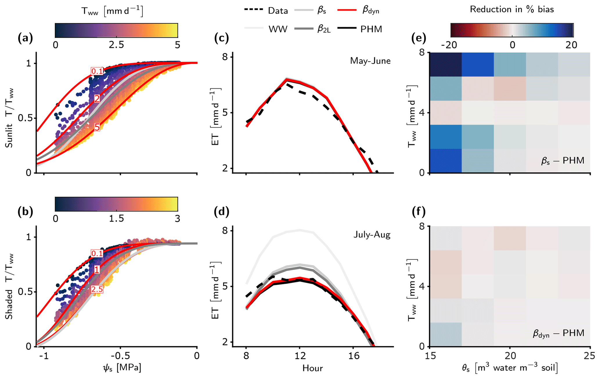
Figure 5 LSM evapotranspiration estimates improved by PHM and new dynamic β. (a–b) Fits of the β_s, β_2L, and β_dyn schemes to the relative transpiration outputs from the calibrated PHM scheme for the sunlit (a) and shaded big leaf (b) of the LSM (see Methods section). Note that only three of the infinite family of β_dyn curves are shown for illustration – each corresponding to a fixed T_ww value in mm d⁻¹ (red numbers). Full fitting details of these three schemes are available in Sect. S6.2. (c–d) The median diurnal ET estimates for the LSM with five transpiration downregulation schemes compared to observations at the US-Me2 AmeriFlux site for early (c) and late summer (d). The dual-source two-big-leaf LSM calculates ET as the sum of sunlit and shaded big-leaf transpiration and ground evaporation. Note that β_dyn (red) is overlying PHM (black) results as they are essentially the same. (e–f) Reduction in absolute percent bias of ET between the β_s and PHM schemes (e) and β_dyn and PHM schemes (f) in terms of atmospheric moisture demand (represented by T_ww) and soil water status (represented by θ_s). In both plots, blue indicates PHM improvement over the selected β scheme.

To aid our comparison of LSM transpiration downregulation schemes, we must first verify that the spectrum of transport limitation found in our minimalist analysis (Sect. 3.1) adequately describes the differences between PHM and β formulations common to TBMs. Our calibrated LSM uses a complex PHM formulation (Sect. 2.2 and Fig. 1b) that partitions the soil–plant–atmosphere continuum into soil-to-xylem, xylem-to-leaf, and leaf-to-atmosphere segments, each with conductance curves that depend nonlinearly (e.g., sigmoidal or Weibull) on water potential. This added complexity does not affect the spectrum of transport limitation (Fig. 4). For clarity, we reiterate two main points from the minimalist PHM analysis found in this complex analysis. First, soil–plant conductance (g_sp) controls whether the soil–plant system is soil-limited (high g_sp; Fig. 4e–f) or transport-limited (low g_sp; Fig. 4a–b) due to non-negligible water potential differences (Δψ) creating large differences between PHMs and β (high ΔT) at intermediate ψ_s values (Fig. 4b, d). Second, for a transport-limited system, ΔT increases with higher variability in atmospheric moisture demand (T_ww), where the importance of “variability” expands on our minimalist results. To clarify, β should be considered an empirical model that could be fit anywhere within the range of the PHM downregulation envelope (light gray shading in Fig. 4b, d, f). Therefore, greater T_ww variability creates a larger PHM downregulation envelope and makes a single β increasingly inadequate for modeling transpiration downregulation.

The consistency between the minimalist and complex PHM suggests that the divergence between PHMs and β in transport-limited systems is not sensitive to the linear or nonlinear forms of supply or demand lines but is rather controlled by the existence of a finite conductance itself. Furthermore, these results strongly support the need to use two independent variables, ψ_s and T_ww (rather than only ψ_s in β), to capture the coupled effects of soil water stress and atmospheric moisture demand on transpiration downregulation in transport-limited soil–plant systems. In light of these findings, we have developed a new dynamic β (β_dyn) that has an additional functional dependence on T_ww (Eq. 16) and compared it against four other downregulation schemes in this LSM analysis.

We now assess the errors incurred by using a β rather than PHM downregulation scheme to model the US-Me2 ponderosa pine site. The median diurnal evapotranspiration (ET; bare soil evaporation plus transpiration) for each LSM version for early summer 2013–2014 indicates that all downregulation schemes perform similarly due to high soil moisture and minimal downregulation (Fig. 5c). However, as soil moisture declines during late summer (Fig. S11) the differences between schemes emerge: the PHM and β_dyn schemes fit the ET observations the best, while β_2L, β_s, and well-watered schemes overpredict ET (Fig. 5d). We explain the poor performance of the static β schemes by plotting the reduction in absolute percent bias between the β_s and PHM schemes (Fig. 5e) with respect to soil water stress (represented by volumetric soil water content measurements at the site, θ_s [m³ water per m³ soil]) and atmospheric moisture demand (represented by T_ww from the well-watered LSM version). The PHM scheme provides substantial percent bias reduction relative to the static β_s scheme under soil water stress (θ_s<0.2) for above- and below-average T_ww values ($T_{\mathrm{ww}}\approx \mathrm{4}\mathrm{mm}{\mathrm{d}}^{-\mathrm{1}}$). This result is true for both static β schemes (β_s and β_2L), because they are fit to the average T_ww behavior over the simulation period (Fig. 5a–b and Sect. S6.2). Therefore, as T_ww becomes higher (lower) than the average, these static β schemes will overpredict (underpredict) transpiration. The PHM also improves performance during wetter soil conditions (θ_s>0.2) with high T_ww – which does not represent typical “drought” conditions – suggesting that PHMs capture transpiration downregulation that β potentially misses as it cannot account for large soil–plant water potential differences (Δψ) under transport limitation and/or high atmospheric moisture demand (similar to Sect. 3.2). Lastly, the near-average T_ww conditions lead to β providing enhanced performance, which can be explained by underlying biases in the calibrated parameter estimates (see Fig. S9).

Notably, the β_dyn downregulation scheme replicates the performance of the PHM scheme by adding a single dimension of T_ww to the original β scheme. This additional dependence on T_ww allows β_dyn to traverse along the PHM downregulation envelope with atmospheric moisture demand changes, whereas the static β schemes are fixed near mean conditions (Fig. 5a–b). The performance difference between PHM and β_dyn schemes is minimal in terms of percent change in bias across all environmental conditions (Fig. 5f; max difference of 3 %), median diurnal variations (Fig. 5c–d), and cumulative flux errors (Table S7–S8; max difference of 0.5 %). Therefore, this additional dependence on T_ww is key to simulating the coupled effects of atmospheric moisture demand and soil water stress in PHMs and accurately modeling transpiration downregulation in transport-limited systems. For this transport-limited system, β_dyn requires two more parameters than the original β scheme, which is half the parameters required for our complex PHM formulation (Sect. S6.2). Furthermore, β_dyn does not require the iterative solution of water potentials and transpiration in PHMs (Sect. 2.2). Rather, it calculates transpiration downregulation algebraically using ψ_s as in the original β. The β_dyn provides a future avenue for correcting existing β model bias without adding the computational and parametric challenges of more realistic PHMs.

4 Discussion and conclusion

The spectrum of transport- and soil-limited transpiration (Fig. 4) explains why many TBMs that use β to represent transpiration downregulation struggle to predict water, energy, and carbon fluxes under soil water stress (Sitch et al., 2008; Powell et al., 2013; Medlyn et al., 2016; Ukkola et al., 2016; Restrepo-Coupe et al., 2017; Trugman et al., 2018) and why implementing PHMs has led to performance improvements (Kennedy et al., 2019; Anderegg and Venturas, 2020; Eller et al., 2020; Sabot et al., 2020). Transpiration in a transport-limited soil–plant system, characterized by finite soil–plant conductance, depends on non-negligible water potential differences to transport water from the soil to the leaf, which result from the joint effects of atmospheric moisture demand and soil water supply on leaf water potential. It is only when the soil–plant conductance becomes infinite (and the system becomes soil-limited) that leaf water potential approximates soil water potential, and transpiration arises as an independent function of soil water supply and atmospheric moisture demand. These are assumptions inherent to the empirical β and explain why β cannot capture the coupled effects of soil water stress and atmospheric moisture demand.

The implications of continued use of β will vary by site. Ecosystems with soil or plant hydraulic properties resistant to flow (e.g., xeric ecosystems, tall trees, species with low xylem conductivity or roots that hydraulically disconnect from the soil during drought) will have large biases depending on the range of soil water availability and atmospheric moisture demand (T_ww) observed at the site (Figs. 3d and 4b). These errors will not be confined to drought periods, as higher atmospheric moisture demand and lower soil–plant conductance can result in errors even during wetter soil conditions (Figs. 3 and 5e). This is a crucial point, given projections indicate diverging degrees of vapor pressure deficit (VPD) stress and soil water stress for ecosystems (Novick et al., 2016). On the other hand, for soil-limited systems (e.g., irrigated crops, riparian vegetation, or groundwater-dependent ecosystems), β may adequately capture transpiration dynamics as soil water status may be a suitable proxy for leaf water status. Therefore, further work must identify the combinations of soil parameters and plant hydraulic traits that define transport- or soil-limited systems to identify ecosystems susceptible to bias from β. Our initial estimates indicate a soil–plant conductance value around 30 $\mathrm{mm}{\mathrm{d}}^{-\mathrm{1}}{\mathrm{MPa}}^{-\mathrm{1}}$ may be a rough threshold for transport limitation (see Sect. S7).

Several other factors not covered in this work could exacerbate the differences between β and PHM predictions. We expect plant capacitance (already incorporated into some TBMs; Xu et al., 2016; Christoffersen et al., 2016) will likely cause further deviations from β. PHMs with capacitance are expected to introduce hysteresis into transpiration downregulation (Zhang et al., 2014) in transport-limited systems that existing β are not equipped to capture. However, this hysteretic behavior may diminish in a high-conductance (i.e., soil-limited) system, because plant and soil water potentials will quickly equilibrate, so β may still be an adequate alternative to a PHM. More advanced representation of stomatal response and plant hydraulic transport could further exacerbate β and PHM differences. Recent advances in optimality-based (Eller et al., 2020; Sabot et al., 2020) and mechanistic stomatal response models (Buckley, 2017) as well as more detailed PHM segmentation (Kennedy et al., 2019) may include additional couplings to plant water and metabolism that cannot be easily approximated by β. Regardless, the core message of this work is still relevant: for transport-limited soil–plant systems, PHMs are necessary to couple the effects of soil water stress and atmospheric moisture demand on transpiration, and β fails because soil water status is not an adequate substitute for leaf water status.

The recognition that a dynamic β model can replicate the complexity of a PHM with half the parameters and more direct computation (Sect. S6.2), simply by adding a dependence on atmospheric moisture demand to the β function, provides a useful pathway for overcoming both the limitations of β and the parametric uncertainties of PHMs (Anderegg and Venturas, 2020; Paschalis et al., 2020). The inadequacies of the static β have been noted since its inception. Feddes et al. (1978), who introduced one of the first β formulations, mentioned β's dependence on atmospheric moisture demand based on field data (Denmead and Shaw, 1962; Yang and de Jong, 1972) and early plant hydraulic theory (Gardner, 1960). Unfortunately, there have been only a few attempts to rectify these inadequacies in the modeling community, short of implementing a full PHM. For example, Feddes and Raats (2004) updated their original β model to vary the water potential at incipient stomatal closure linearly with atmospheric moisture demand, which has been adopted in the field-scale SWAP model (Kroes et al., 2017), while the Ecosystem Demography-2 model (Medvigy et al., 2009) uses a sigmoidal function for transpiration downregulation that contains the ratio of soil water supply to evaporative demand. Within many TBMs and hydrological models, a dynamic β could easily replace the original β by allowing existing fixed parameters to vary with T_ww (already calculated in many transpiration downregulation schemes). In addition to improving TBM performances, dynamic β also has the potential to aid in remote sensing retrievals and indirect inferences of land surface fluxes. Currently, the state-of-the-art ECOSTRESS (ECOsystem Spaceborne Thermal Radiometer Experiment on Space Station) experiment provides global ET estimates based on a modified Priestley–Taylor formulation that uses a β function to downregulate ET under soil water stress (Fisher et al., 2020). These spaceborne products could easily implement the dynamic β formulation to correct biases for many transport-limited ecosystems. These potential applications rely on formalizing the relationship between the dynamic β parameters and their dependence on T_ww. As it stands, the dynamic β still needs to be calibrated to site-specific data; however, it provides a physically informed alternative to PHMs with less calculation and fewer parameters. Further work will focus on generalizing the dynamic β by linking its parameters to measurable soil properties, plant hydraulic traits, and atmospheric feedbacks.