Assimilation of probabilistic flood maps from SAR data into a coupled hydrologic–hydraulic forecasting model: a proof of concept

Coupled hydrologic and hydraulic models represent powerful tools for simulating streamflow and water levels along the riverbed and in the floodplain. However, input data, model parameters, initial conditions, and model structure represent sources of uncertainty that affect the reliability and accuracy of flood forecasts. Assimilation of satellite-based synthetic aperture radar (SAR) observations into a flood forecasting model is generally used to reduce such uncertainties. In this context, we have evaluated how sequential assimilation of flood extent derived from SAR data can help improve flood forecasts. In particular, we carried out twin experiments based on a synthetically generated dataset with controlled uncertainty. To this end, two assimilation methods are explored and compared: the sequential importance sampling method (standard method) and its enhanced method where a tempering coefficient is used to inflate the posterior probability (adapted method) and reduce degeneracy. The experimental results show that the assimilation of SAR probabilistic flood maps significantly improves the predictions of streamflow and water elevation, thereby confirming the effectiveness of the data assimilation framework. In addition, the assimilation method significantly reduces the spatially averaged root mean square error of water levels with respect to the case without assimilation. The critical success index of predicted flood extent maps is significantly increased by the assimilation. While the standard method proves to be more accurate in estimating the water levels and streamflow at the assimilation time step, the adapted method enables a more persistent improvement of the forecasts. However, although the use of a tempering coefficient reduces the degeneracy problem, the accuracy of model simulation is lower than that of the standard method at the assimilation time step.

1 Introduction

Floods represent one of the major natural disasters with a global annual average loss of USD 104 billion (UNISDR, 2015). The extent of flood damages have risen over the last few years due to climate-driven changes and an increase in the asset values of floodplains (Blöschl et al., 2019). This emphasizes the need for reliable and cost-effective flood forecasting models to predict flood inundations in near real time. Hydrologic and hydraulic models represent useful tools for simulating flood extent, discharge, and water levels in the riverbed and on the floodplain. However, both the models and the observations used as inputs for running, calibrating, and evaluating the models are affected by uncertainty.

Data assimilation (DA) aims at improving model predictions by updating model states and/or parameters based on observations (Moradkhani et al., 2005). It optimally combines observations with the system state derived from a numerical model accounting for both model and observation errors.

Ideally, in situ data are systematically assimilated into flood forecasting models, but these observations are not always available (e.g., in un-gauged catchments) and only provide space-limited information (Grimaldi et al., 2016). Therefore, satellite Earth observation (EO) data, and in particular synthetic aperture radar (SAR) images, represent a valuable complementary dataset to in situ observations due to their capacities to provide frequent updates of flooded areas at a large scale. In addition, as the corresponding EO data archives are growing fast, historical observational data spanning an extended period of time can be assimilated into large-scale hydrodynamic models.

SAR sensors are able to acquire images of flooded areas and permanent water bodies during day and night almost regardless of weather conditions. The backscattered signal depends on the dielectric properties of the imaged objects. Smooth surfaces, such as open water bodies, interact with the transmitted pulse so that a very limited part of the signal is backscattered to the satellite resulting in dark areas in the acquired image.

Different information about water extent can be extracted from a SAR image and used to improve the forecasts using DA techniques. Directly assimilating flood extent maps is not straightforward because these do not correspond to a state variable of the model. Therefore, some studies suggested transforming the SAR backscatter information into a state variable prior to the assimilation. For instance, several studies have used EO-derived water levels to improve flood forecasts (e.g., Andreadis et al., 2007; García-Pintado et al., 2015; Matgen et al., 2010; Revilla-Romero et al., 2016; Giustarini et al., 2011; Hostache et al., 2010). The water levels are estimated by merging pre-selected flood extent limits extracted from the SAR satellite imagery with a digital elevation model (DEM). This step requires precise flood contour maps and high-resolution DEMs, which are not always available (Hostache et al., 2018).

In the existing literature only a few studies have used DA for directly assimilating flood extent maps into flood forecasting models (e.g., Lai et al., 2014; Revilla-Romero et al., 2016; Cooper et al., 2019, 2018; Hostache et al., 2018). Among the advantages of a direct use of the SAR backscatter values is that it reduces the data processing time, which is a key element in near-operational applications.

Cooper et al. (2018) have used an ensemble Kalman filter to update a 2D hydrodynamic model. In this case, the backscatter values are directly assimilated into the model without being transformed into state variables of the flood forecasting system. The dry and wet pixels of the simulated binary flood map are converted into equivalent SAR backscatter values corresponding to the spatial mean of the SAR backscatter observations. Cooper et al. (2018) showed that the SAR backscatter-based assimilation method performs well compared to the assimilation method where the SAR backscatter is transformed into water levels.

Hostache et al. (2018) used a variant of the particle filter (PF) with sequential importance sampling (SIS) to assimilate probabilistic flood maps (PFMs) derived from SAR data into a coupled hydrologic–hydraulic model with the assumption that rainfall is the main source of uncertainty together with SAR observations.

Their study showed that the assimilation of PFMs is beneficial: the number of correctly predicted flooded pixels increases as compared to the case without any assimilation, hereafter called open loop (OL). Forecast errors are reduced by a factor of 2 at the assimilation time and improvements persist for subsequent time steps up to 2 d. However, the improvements are not systematic: for some cases the updated hydraulic output deviates from the observations. One of the reasons for such outliers could be the assumption that rainfall represents the dominating source of uncertainty together with satellite observation errors, thereby excluding other possible sources of uncertainty in the model system such as input data, model parameters, initial conditions, and model structure. Even though the assumption seems to be rather realistic and suitable in operational cases, given that rainfall uncertainty has been generally identified as one of the major causes of poorly performing models (Koussis et al., 2003; Pappenberger et al., 2005), coupled models may have additional sources of uncertainty affecting the results.

The present study is a follow up of the real-world experiment by Hostache et al. (2018) and carries out a similar experiment in a controlled environment that considers the estimated rainfall together with SAR observations as the only sources of uncertainty.

Hostache et al. (2018) also highlighted that degeneracy may be a major issue for PFs: after the assimilation, the number of particles with high weights reduces to a few or only one particle so that the ensemble loses statistical significance. To overcome this issue, Hostache et al. (2018) used a site-dependent tempering coefficient that inflates the posterior probability. In our study, we propose to adopt an enhanced tempering coefficient as a function of the desired effective ensemble size (EES) after the assimilation.

Moreover, in Hostache et al. (2018), speckle errors in the SAR observations are taken into account through the Bayesian approach introduced by Giustarini et al. (2016). However, no conclusions are drawn concerning the effect of misclassified pixels. In fact, for some particular cases such as densely vegetated areas, the detection of floodwater from SAR imagery is known to be prone to errors. Detecting and removing such errors represents one of the main scientific challenges of using SAR data for a systematic, fully automated, large-scale flood monitoring (and prediction).

The main objective of the present study is to assess the strengths and the limitations of the DA framework previously proposed by Hostache et al. (2018). To do that we evaluate the DA framework in a fully controlled environment via synthetic twin experiments as this shall allow us to draw unambiguous and comprehensive conclusions. In addition, we conduct a sensitivity analysis of the DA framework with respect to the critical tempering coefficient that was recently introduced for tackling degeneracy more efficiently. We also aim to evaluate the effect of misclassified SAR pixels on DA. Therefore, errors are artificially added within the SAR image with the aim of getting a better understanding on how robust the proposed method is with respect to these types of errors. The results are evaluated not only locally but also over the entire flood domain and for subsequent time steps to the assimilation. To carry out the experimental study we apply the DA framework to a forecasting system consisting of a loosely coupled hydrologic model (SUPERFLEX) and hydraulic model (LISFLOOD-FP). The meteorological data that are used to run the experiments are derived from the ERA5 archive with a spatial resolution of 25 km and a temporal resolution of 1 h. The SAR data are synthetically generated with a pixel spacing of 75 m.

2 Methods

The proposed methodology is based on numerical experiments conducted with synthetically generated data as illustrated in the flow chart given in Fig. 1. In this framework, the following data inputs and models are employed:

1. True rainfall time series are used to generate the true hydrologic–hydraulic model simulation.

2. Synthetic SAR observations are generated from the true model run (i.e., from the simulated flood extent map).

3. The true rainfall time series are randomly perturbed and used as inputs of the hydrologic model. The simulated discharge data are then used as boundary conditions to produce an ensemble of hydraulic model runs.

4. The synthetic SAR observations are assimilated into the coupled hydrologic–hydraulic model via different variants of the particle filter (PF).

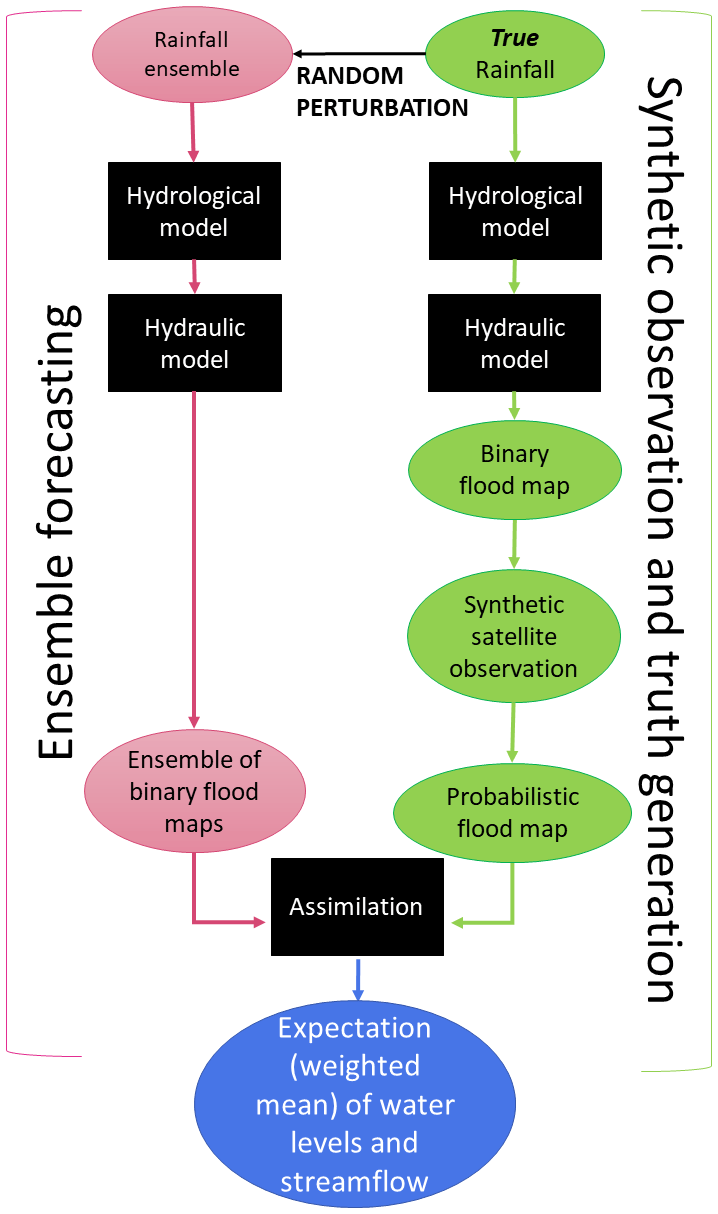
Figure 1 Flow chart of the synthetic experiment. The true rainfall is perturbed. The same flood forecasting model structure composed of a hydrologic model and a hydraulic model is used to obtain the probabilistic flood map and the ensemble of binary flood maps. The probabilistic flood map is assimilated into the ensemble of binary flood maps via the particle filter to obtain the weights with which the expectation of water levels, streamflow, and flood extents are computed.

The three conducted experiments are summarized as follows:

• a.

  An application of the standard PF where degeneracy occurs.

• b.

  An application of the adapted PF where a tempering coefficient is used to reduce degeneracy. We also investigated the sensitivity of the DA results to different values for the tempering coefficient, corresponding to the EES of 5 %, 10 %, 20 %, and 50 %.

• c.

  An application of both proposed methods with artificially introduced known errors into the SAR image classification in order to evaluate the impact of these errors on the DA performance metrics.

2.1 Coupled hydrologic–hydraulic model: synthetic truth and ensemble

The coupled modeling system consists of a hydrologic model coupled with a hydraulic model. The hydrologic model is used to compute the runoff at the upstream boundaries of the hydraulic model. The hydrologic model used in this study is SUPERFLEX, which is a framework for conceptual hydrologic modeling introduced by Fenicia et al. (2011). The model structure is a combination of generic components: reservoirs, connection elements, and lag functions. In this study, a lumped conceptual model and its structure as a combination of three reservoirs are used: an unsaturated soil reservoir with storage S_UR, a fast-reacting reservoir with storage S_FR, and a slow-reacting reservoir with storage S_SR. A lag function has been added at the outlet of the slow- and fast-reacting reservoirs.

The hydraulic model is based on LISFLOOD-FP (Bates and Roo, 2000; Neal et al., 2012) and simulates flood extent, water levels, and streamflows along the river and on the floodplain. A sub-grid 1D kinematic solver is used for the channel flow. When the storage capacity of the river is exceeded, the water spills into the floodplain and a 2D diffusion wave scheme neglecting the convective acceleration (de Almeida and Bates, 2013; Bates et al., 2010) is used for the floodplain flow simulation.

The true meteorological data (i.e., temperature and rainfall) are used as input for the hydrologic–hydraulic model to simulate streamflow and water level time series and to provide binary flood maps, where each pixel is classified as flooded (with value 1) or non-flooded (with value 0) at each assimilation time step. These computational results represent the synthetic truth that will be used to evaluate the performance of the proposed assimilation framework. The true binary flood maps are also used to generate the synthetic SAR observations as described in the next section.

2.2 Synthetic observations

In the proposed synthetic experiment, we generate synthetic SAR images at each assimilation time step. The SAR images are generated with the same spatial resolution of the LISFLOOD-FP maps. Similarly to the Van Wesemael (2019) study, we make use of a real SAR image, acquired during a flood event in the past, and of the LISFLOOD-FP model to generate true binary flood maps. The histogram of the SAR image backscatter values can be approximated with two Gaussian curves relative to the flooded and non-flooded pixel classes. Generally, the class of flooded pixels is often represented just by a fraction of the SAR image scenes. Therefore, to identify and characterize areas where the flooded and non-flooded classes are more balanced, the hierarchical split-based approach (HSBA; Chini et al., 2017) is applied to the selected SAR image. The parameters of the Gaussian PDFs are determined by fitting the histogram values of the HSBA selected areas.

Then, random backscatter values, derived from the calibrated Gaussian PDFs, are associated with the pixels of the true binary flood map indicating the presence of water and no-water areas. Once the synthetic SAR images are generated, the Giustarini et al. (2016) procedure is applied and synthetic PFMs are derived. The probability of being flooded, given the recorded backscatter values for each pixel of a SAR image p(F|σ⁰), is obtained via the Bayes' theorem:

$$\begin{array}{}\text{(1)}& \begin{array}{rl}p\left(F|{\mathit{\sigma }}^{\mathrm{0}}\right)& ={\displaystyle \frac{p\left({\mathit{\sigma }}^{\mathrm{0}}|F\right)p\left(F\right)}{p\left({\mathit{\sigma }}^{\mathrm{0}}\right)}}\\ & ={\displaystyle \frac{p\left({\mathit{\sigma }}^{\mathrm{0}}|F\right)p\left(F\right)}{p\left({\mathit{\sigma }}^{\mathrm{0}}|F\right)p\left(F\right)+p\left({\mathit{\sigma }}^{\mathrm{0}}|\stackrel{\mathrm{‾}}{F}\right)p\left(\stackrel{\mathrm{‾}}{F}\right)}}.\end{array}\end{array}$$

In Eq. (1), p(σ⁰|F) and $p\left({\mathit{\sigma }}^{\mathrm{0}}\right|\stackrel{\mathrm{‾}}{F})$ represent, respectively, the probability of the backscatter values of the flooded and non-flooded pixels, p(F) is the prior probability of a pixel being flooded, and $p\left(\stackrel{\mathrm{‾}}{F}\right)$ is the prior probability of a pixel being non-flooded before any backscatter information is taken into account. The conditional probabilities are derived from the histogram of the backscatter values estimated from the synthetically generated SAR image. The prior probabilities can be estimated from the flood extent model output or through visual interpretation of aerial photography in real cases. However, in general such information is not always available and the prior probabilities are unknown. Consequently, Giustarini et al. (2016) set the prior probability of Eq. (1) to 0.5 so that both flooded and non-flooded pixels are equally likely. While this study is based on a synthetic experiment, true binary flood extent maps are available. Therefore, the assimilation is realized using both the estimated prior probability (as the ratio between the flooded area and the total area) and the prior probability equal to 0.5. Given the similarity of the results for both cases, in the following sections we only discuss the experiment using the estimated prior probability.

The method proposed by Giustarini et al. (2016) aims to characterize the speckle-induced uncertainty. However, it does not consider any other phenomena leading to a wrong classification in SAR-based flood maps. Particular atmospheric conditions (e.g., wind, snow, and precipitation), water-lookalike areas (e.g., asphalt, sand, and shadow), or obstructing objects (e.g., dense canopy and buildings), as mentioned in Giustarini et al. (2015), can lead to a wrong classification in the flood maps. Therefore, the areas where such errors could occur should be masked out from the SAR-based flood maps in order to provide reliable flood detection.

In the first part of this study, SAR observations are considered without errors. In the second part, these kinds of errors are integrated in the synthetic SAR observations to evaluate their effect on the DA. Specifically, the pixels along the flood edge of each particle are selected. From this set, a given number of those pixels effectively flooded in the true binary flood map are artificially corrupted so that they belong to dry pixels. The number of corrupted pixels depends on the magnitude of the error that we want to introduce in the SAR observations.

2.3 Ensemble generation

In a PF, the prior and posterior PDFs are approximated by a set of particles. Here, we hypothesize that rainfall is the only source of uncertainty affecting the model-based flood extent simulations. For this reason, an ensemble of rainfall time series is used as input for the coupled hydrologic–hydraulic model. Each rainfall time series is obtained by perturbing, with a multiplicative random noise from a log-normal error distribution, the true rainfall time series following the approach proposed in Hostache et al. (2018). Via the hydrologic model, 128 rainfall time series are obtained and forwarded in time.

It is important to note that the same hydrologic–hydraulic model in terms of structure, initial conditions, and parameters is used for all model runs. The reliability of the rainfall ensemble is verified with the statistical metrics proposed by De Lannoy et al. (2006). According to the verification measurement VM₁ in Eq. (2):

$$\begin{array}{}\text{(2)}& {\mathrm{VM}}_{\mathrm{1}}={\displaystyle \frac{<\mathrm{ensk}>}{<\mathrm{ensp}>}}\approx \mathrm{1}.\end{array}$$

The ensemble spread in Eq. (3) (where x_k,n represents the value of the variable x at time k for each pixel n)

$$\begin{array}{}\text{(3)}& {\mathrm{ensp}}_k={\displaystyle \frac{\mathrm{1}}{N}}\sum _{n=\mathrm{1}}^N{\left(x_{k,n}-{\stackrel{\mathrm{‾}}{x}}_k\right)}^{\mathrm{2}}\end{array}$$

has to be close to the ensemble skill (Eq. 4)

$$\begin{array}{}\text{(4)}& {\mathrm{ensk}}_k=\left({\stackrel{\mathrm{‾}}{x}}_k-y_k\right),\end{array}$$

which is the difference between the mean ${\stackrel{\mathrm{‾}}{x}}_k$ over the N particles of the ensemble and the observation y_k at time k. VM₂ (Eq. 5) verifies that the truth is statistically indistinguishable from the random samples of the ensemble.

$$\begin{array}{}\text{(5)}& {\mathrm{VM}}_{\mathrm{2}}={\displaystyle \frac{<\mathrm{ensk}>}{<\mathrm{mse}>}}\approx {\displaystyle \frac{(N+\mathrm{1})}{\mathrm{2}N}}\end{array}$$

with “mse” estimated as:

$$\begin{array}{}\text{(6)}& {\mathrm{mse}}_k={\displaystyle \frac{\mathrm{1}}{N}}\sum _{n=\mathrm{1}}^N{\left(x_{k,n}-y_k\right)}^{\mathrm{2}}.\end{array}$$

VM₁ and VM₂ are used to assess the quality of the discharge ensemble at the output of the hydrologic model.

2.4 Data assimilation framework

The DA framework consists of two main steps: prediction, i.e., model simulations, and analysis, i.e., update of particle probabilities when an observation is available. The prior probability of the model state x at a given time k is represented by a set of N independent random particles x_n sampled from the prior probability distribution p(x) as

$$\begin{array}{}\text{(7)}& p\left(x\right)={\displaystyle \frac{\mathrm{1}}{N}}\sum _{n=\mathrm{1}}^N\mathit{\delta }\left(x-x_n\right),\end{array}$$

where δ is the Dirac delta function. In this study, the prior probability distribution is assumed to be uniform. The observations of flooded or non-flooded pixels y are related to the true state x^t according to the following equation:

$$\begin{array}{}\text{(8)}& y=H\left[x^t\right]+\mathit{ϵ},\end{array}$$

where H is the observation operator that maps the state vector into the observation space and ϵ represents the observation errors. According to the Bayes' theorem, the observations are assimilated by multiplying the prior PDF p(x) and the likelihood p(y|x), which is the probability density of the observation given the model state, and dividing by the total probability p(y), resulting in

$$\begin{array}{}\text{(9)}& p\left(x\right|y)={\displaystyle \frac{p\left(y\right|x)}{p\left(y\right)}}p(x),\end{array}$$

which is the posterior probability p(x|y), i.e., the probability density function of the model state given the observations. By inserting Eq. (7) into Eq. (9) we obtain the following formula:

$$\begin{array}{}\text{(10)}& p\left(x\right|y)\approx \sum _{n=\mathrm{1}}^N{W}_n\mathit{\delta }\left(x-x_n\right),\end{array}$$

where W_n represents the relative importance in the probability density function (i.e., global weight) given by

$$\begin{array}{}\text{(11)}& W_n={\displaystyle \frac{p\left(y|x_n\right)}{N\cdot p\left(y\right)}}={\displaystyle \frac{p\left(y|x_n\right)}{N\cdot \int p\left(y\right|x\left)p\right(x)\mathit{\delta }x}}\approx {\displaystyle \frac{p\left(y|x_n\right)}{\sum p\left(y|x_j\right)}}.\end{array}$$

In this study, the likelihood (global weight, W_n) is represented by the product of the pixel-based likelihood (local weight, w_i), assuming the L pixel observation errors are independent from each other. At time k of the observation, local weights w_i,n are defined for each particle n and for each pixel i according to Hostache et al. (2018):

$$\begin{array}{}\text{(12)}& w_{i,n}=p_i\left(F|{\mathit{\sigma }}_{\mathrm{0}}\right)M_{i,n}+\left[\mathrm{1}-p_i\left(F|{\mathit{\sigma }}_{\mathrm{0}}\right)\right]\left(\mathrm{1}-M_{i,n}\right).\end{array}$$

w_i,n is equal to the probability of a pixel being flooded as derived from the synthetically generated SAR image. M_i,n is equal to 1 if the model predicts the pixel as flooded, whereas M_i,n is equal to 0 if the model predicts the pixels as non-flooded. We convert the model-based water depth maps into binary flood extent maps by considering that a pixel is flooded if its water level is above 10 cm. p_i(F|σ₀) equals the probability of a pixel being flooded according to the observations, on conversely $\mathrm{1}-p_i\left(F\right|{\mathit{\sigma }}_{\mathrm{0}})$ equals the probability of not being flooded. By applying Eq. (12) we assign higher probabilities to those pixels where model predictions and observations agree. Next, W_n is estimated for each particle by the normalization of the product of the local weights ensuring that the sum of the global weights is equal to 1 (Eq. 13; standard method).

$$\begin{array}{}\text{(13)}& W_n={\displaystyle \frac{\prod _{i=\mathrm{1}}^L{w}_{i,n}}{\sum _{n=\mathrm{1}}^N\prod _{i=\mathrm{1}}^L{w}_{i,n}}}\end{array}$$

The expectation of the OL is equivalent to the mean of the ensemble because the relative importance of each particle is the same. The global weights are used to compute the expectation of the streamflows (Q) and water levels (h) at time (k) and per pixel (i) after the assimilation (see Eqs. 14 and 15).

$$\begin{array}{}\text{(14)}& {\displaystyle }& {\displaystyle }{\stackrel{\mathrm{‾}}{h}}_i=\sum _{n=\mathrm{1}}^N{W}_n\cdot h_{i,n}\text{(15)}& {\displaystyle }& {\displaystyle }{\stackrel{\mathrm{‾}}{Q}}_i=\sum _{n=\mathrm{1}}^N{W}_n\cdot Q_{i,n}\end{array}$$

The particles keep these global weights until the next assimilation time. The particles are then set to the same equal weight before a new analysis step is performed.

Unless the number of particles increases exponentially with the dimension of the system state, the particle filter is likely to degenerate because high probability is assigned to a single particle while all other members will result in small weights (van Leeuwen et al., 2019). PFs are often subject to degeneracy issues when, due to computational reasons, the number of particles is not sufficiently high (Zhu et al., 2016). After the application of the standard PF, the variance of the weights tend to increase and only a few particles of the ensemble have a non-negligible weight. To mitigate this problem, in Hostache et al. (2018), the global weight defined in Eq. (13) has been adapted using a tempering coefficient (α, as described by the following Eq. 16).

$$\begin{array}{}\text{(16)}& W_n\left(\mathit{\alpha }\right)={\displaystyle \frac{\prod _{i=\mathrm{1}}^L{w_{i,n}}^{\mathit{\alpha }}}{\sum _{n=\mathrm{1}}^N\prod _{i=\mathrm{1}}^L{w_{i,n}}^{\mathit{\alpha }}}}\end{array}$$

Since α and weights values are lower than 1, adding the power of α in the weights formula allows for shifting all weight values closer to 1. This therefore decreases the variance of the weights and inflates the posterior probability. After the assimilation, the number of particles with significant weight depends on the α value. The smaller the α, the higher the variance of the posterior PDF. Consequently, as argued in Hostache et al. (2018), when the α coefficient is small enough, this adaptation of the PF helps reduce the degeneracy of the ensemble. While in the previous study by Hostache et al. (2018) the α value was defined so that the worst model solution would have had a non-zero global weight, in this study we propose to define α based on the desired effective ensemble size (EES). The coefficient α in Hostache et al. (2018) is site-dependent as it relies on the number of flooded pixels, whereas in this study α is a function of the EES, which is a measure of degeneracy based on the global weights (Arulampalam et al., 2002):

$$\begin{array}{}\text{(17)}& \mathrm{EES}\left(\mathit{\alpha }\right)={\displaystyle \frac{\mathrm{1}}{\sum _{n=\mathrm{1}}^N{\left(W_n\left(\mathit{\alpha }\right)\right)}^{\mathrm{2}}}}\cdot {\displaystyle \frac{\mathrm{1}}{N}}\cdot \mathrm{100}.\end{array}$$

The EES is lower than N and its value indicates the level of degeneracy. α is equal to 1 when the standard method is used. Decreasing the α coefficient leads to an increase of the EES.

2.5 Performance metrics

To carry out the evaluation of the PFM statistics we have used reliability plots. The results of the different assimilation scenarios are evaluated on a spatiotemporal scale with the following performance metrics:

• contingency maps and the confusion matrix

• critical success index (CSI)

• root mean square error (RMSE)

• discharge and water level time series.

2.5.1 Reliability plots

Reliability diagrams are employed to statistically evaluate the synthetically generated PFMs. In such diagrams, the probability range [0; 1] is subdivided into intervals of average probability P_i and width ΔP_i. We identify the pixels Ω_i having a probability value of P_i±ΔP_i in the PFM. The fraction of Ω_i pixels effectively flooded in the binary truth map are identified with F_i. The reliability diagram plots P_i on the x axis and F_i on the y axis. A reliability diagram indicating an alignment of data points close to the 1:1 line means that the PFM is statistically reliable.

2.5.2 Contingency maps and confusion matrix

First, we use contingency maps to graphically compare the expected flood map with the synthetic truth map at each assimilation time step. Pixel classification errors can be of two types: overprediction (type error I), when the pixels in the truth map are non-flooded but are predicted as flooded, and underprediction (type error II) in the opposite case. Then, the confusion matrix numerically summarizes the results of the contingency map. It is a 2 rows by 2 columns matrix that reports the number of false positives (type I error), false negatives (type II error), true positives, and true negatives.

2.5.3 CSI

The CSI evaluates the goodness of fit between the truth map and the predicted flood extent map (Bates and Roo, 2000):

$$\begin{array}{}\text{(18)}& \mathrm{CSI}={\displaystyle \frac{A}{A+B+C}}.\end{array}$$

It represents the ratio between the number of pixels correctly predicted as flooded (A) over the sum of all the flooded pixels including the false positives (B; overdetection) and false negatives (C; underdetection). The CSI ranges between 0 and 1 (best score). We also used it to evaluate the results at the assimilation time step and the effect of the assimilation at subsequent time steps. It has been also used to evaluate performance when errors are added in the SAR observations.

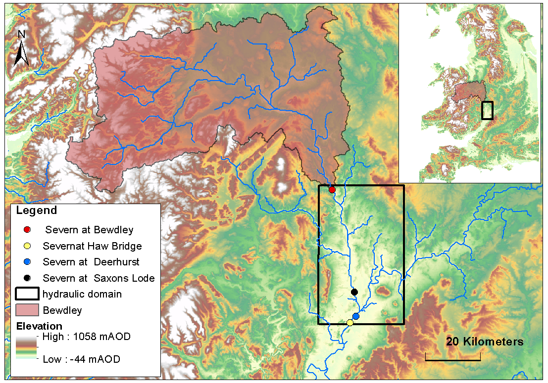
Figure 2 Study area: river Severn (UK). Only the boundary condition in Bewdley is taken into account. Within the sub-catchment upstream of Bewdley a lumped hydrologic model is used to determine the input for the hydraulic model along the river Severn downstream. The dots represent the existing gauging stations where the performance of the DA framework is evaluated. The black square is the hydraulic domain where LISFLOOD-FP runs.

2.5.4 RMSE

The RMSE is considered an excellent error metric for numerical predictions. The RMSE measures the square root of the average square error of the predicted water levels ($h_k^{\mathrm{p}}$) against the truth ($h_k^{\mathrm{t}}$) per pixel k over the total number of pixels L of the flood domain.

$$\begin{array}{}\text{(19)}& \mathrm{RMSE}=\sqrt{{{\displaystyle \frac{\sum _{i=\mathrm{1}}^L\left(h_i^{\mathrm{p}}-h_i^{\mathrm{t}}\right)}{L}}}^{\mathrm{2}}}\end{array}$$

In this study, the RMSE is a measure of the global accuracy of the flood forecasting model predictions of water levels, allowing us to compare prediction errors of the different assimilation scenarios over the flood domain. The RMSE is evaluated at the assimilation time and also at subsequent time steps. It has been also used to evaluate performance when errors are added in the SAR observations.

3 Study area and data

Our synthetic experiment is grounded on a real test site and an actual storm event: the river Severn in the mid-west of the UK (Fig. 2) and the July 2007 flood event, respectively. This area has experienced several floods along the river valleys (Environment Agency, 2009) generally due to intense precipitation.

While seven upstream catchments contribute to the flow along the river Severn, in our study only one upstream catchment is considered: the river Severn at the Bewdley gauging station. Our first objective is to evaluate whether the model correctly predicts the output in the simplest case, i.e., when a unique runoff input to the hydraulic model determines the flood extent and no additional contributing tributaries interfere.

The ERA5 dataset (Hersbach et al., 2018) referring to the period of July 2007 has been used in this experiment. ERA5 is a global atmospheric re-analysis dataset provided by the European Centre for Medium-Range Weather Forecasts (ECMWF). Rainfall and 2 m air temperature at a spatial resolution of approximately 25 km and a temporal resolution of 1 h are used as input to the hydrologic model. The true rainfall time series is used to generate the true runoff before being perturbed in order to obtain 128 different particles as inputs to the hydrologic model. The boundary condition of the hydraulic model is imposed in the corresponding red dot in Fig. 2. Channel width, channel depth, slope of terrain, friction of the flood domain, and channel bathymetry are defined in each cell of the model domain as described in Wood et al. (2016). A uniform flow condition is imposed downstream. No lateral inflow in the hydraulic model is assumed. Finally, at each time step a stack of 128 wet/dry maps is obtained. Discharges and water levels recorded at different gauging stations (corresponding to the existing ones; dots in Fig. 2) along the river are used to evaluate the performance of the DA.

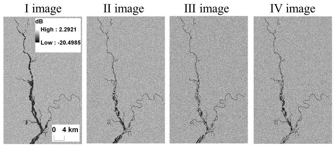
Figure 3 Detail of the synthetic SAR images corresponding to the four assimilation time steps. Darker pixels correspond to lower backscatter.

Figure 4 Details of the synthetic probabilistic flood maps are derived from synthetic SAR images. The probabilities of being flooded given the SAR backscatter values go from low values (yellow) to high values (blue).

4 Results

4.1 Synthetic SAR and ensemble generation and evaluation

The virtual satellite acquisition dates are aligned with the actual Sentinel-1 acquisition frequency. The revisit time over Europe, considering both ascending and descending orbits, is around 3–4 d, meaning that on average two satellite images are available per week. In order to adopt a realistic Sentinel-1-like observation scenario we chose to assimilate four synthetic observations over a period of 10 d.

In Figs. 3 and 4, the area corresponds to the hydraulic model domain. The hydrologic model, covering the upstream catchment, is used to compute the input boundary conditions of the hydraulic model. The results are computed and compared within the hydraulic model domain. The synthetic SAR observations are shown in Fig. 3. The corresponding PFMs are shown in Fig. 4 and reliability plots are provided in Fig. 5. In the reliability plots, the points aligned along the 1:1 line indicate a statistically reliable PFM.

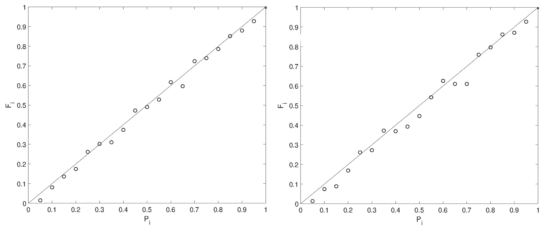
Figure 5 Example of the reliability plots for the verification of the synthetic probabilistic flood maps of the first two synthetic SAR images. On the x axis is the probability range (P_i) and on the y axis is the fraction of pixels within the probability range of the probabilistic flood map observed as flooded in the true binary flood map (F_i). The probabilistic flood maps are statistically reliable because the points align along the 1:1 line.

The verification measurements VM₁ and VM₂ (Eqs. 2 and 5) of the ensemble discharge in Bewdley (Fig. 6) are equal to 1.047 and 0.527, respectively. These values are close to the ideal values of 1 and 0.5.

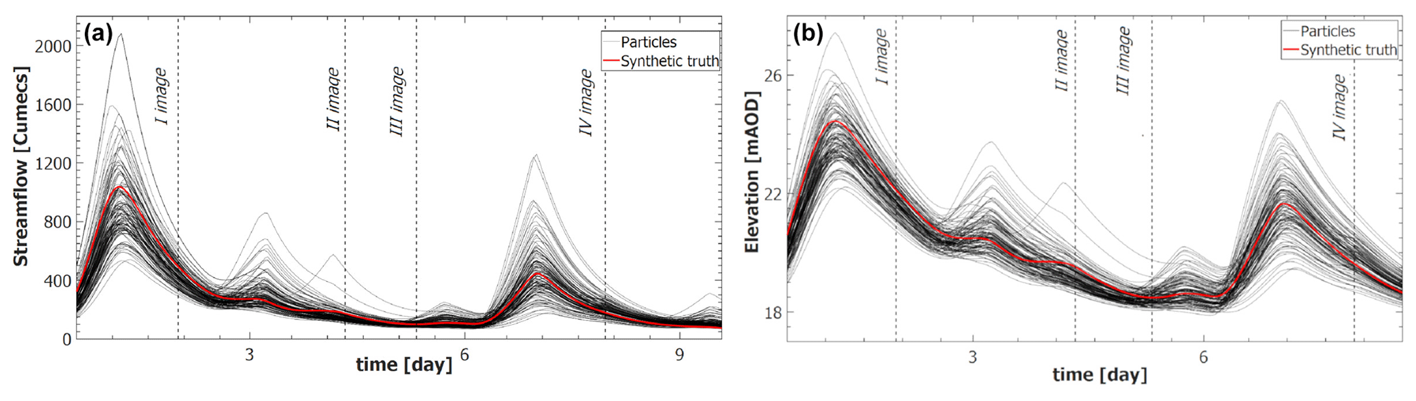
Figure 6 Streamflow time series (a) and water elevation time series (b) at the gauge station in Bewdley. Black lines represent the 128 particles while the red line corresponds to the synthetic truth.

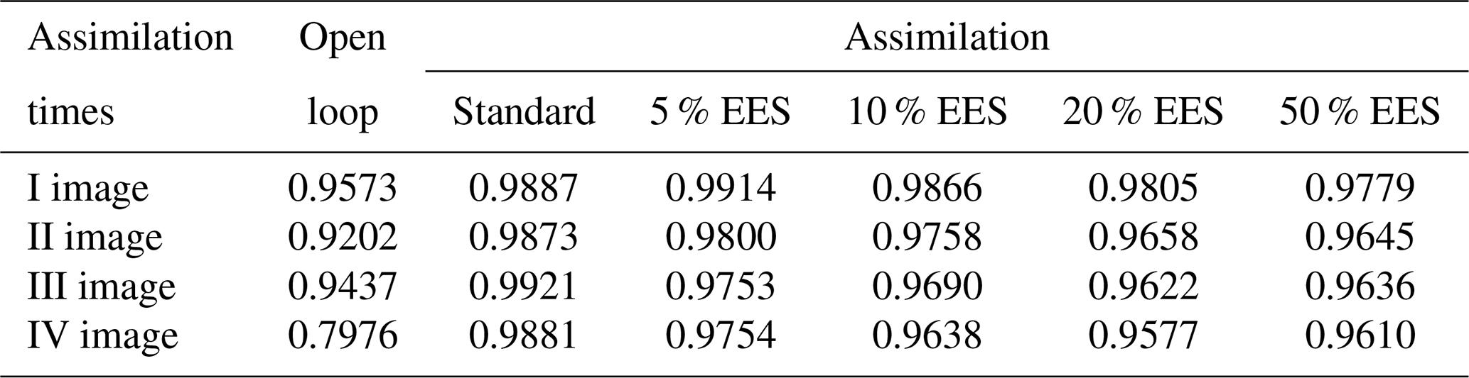
Table 1 Critical success index values at each assimilation time step. The open loop (Fig. 6) where no assimilation is computed is compared with the standard method and the adapted method with an increasing effective ensemble size (EES).

4.2 Evaluation of the flood extent map estimated at the assimilation time

The CSI is computed over the entire hydraulic model domain at each assimilation time step.

The general trend of the assimilation effect is positive, as errors tend to decrease at all the assimilation steps with different assimilation methods. Even though the CSI is already high with the OL, the assimilation further improves the results and this becomes particularly clear at the last assimilation time step. From Table 1 it can be noticed that the CSI, approximately equal to 0.80 with the OL in the worst case (assimilation of the IV image), exceeds 0.96 for the different assimilation types and reaches the maximum value of 0.99 with the standard method. In Fig. 7, we provide the contingency maps of the OL and of the 5 % EES approach (results of the standard method are similar to those of the 5 % EES approach and therefore not shown). For each pair of images, we show on the left the results of the OL and on the right the results obtained after the assimilation.

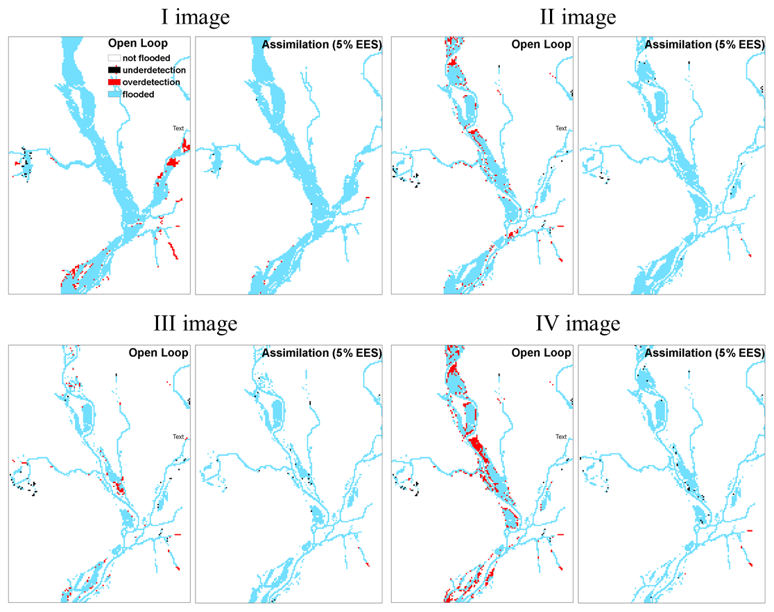
Figure 7 Contingency maps before (open loop) and after assimilation at 5 % EES at each time step. Two types of errors can be distinguished: overdetection (red pixels) when the model predicts the pixel as flooded but the pixel is observed as non-flooded and underdetection (black pixels) when the contrary occurs. When the model and observations agree, pixels are correctly classified as non-flooded (white pixels) and flooded (blue pixels).

In this study, it can be observed that the OL has a tendency to overdetection; the number of red pixels is higher than the number of black pixels and after the assimilation the number of overdetected pixels decreases, confirming the results obtained with the CSI.

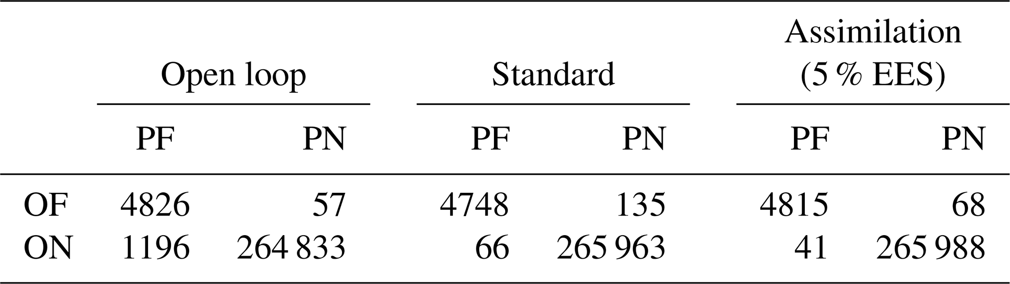
The confusion matrix given in Table 2 provides more details on the fourth assimilation time step. On one hand, the number of pixels wrongly predicted as flooded in the OL is 1196 and more than 90 % of these are correctly classified as non-flooded after the assimilation for both the standard and 5 % EES methods. On the other hand, a few pixels correctly predicted as flooded in the OL are classified as non-flooded after the assimilation. However, it can be argued that the number of 201 wrongly classified pixels after the assimilation is rather low compared to the 1253 px of the OL.

Table 2 Confusion matrix of the OL and of the 5 % EES assimilation at the fourth assimilation time step (OF = observed flooded pixels in the truth map, ON = observed non-flooded pixels in the truth map, PF = predicted flooded pixels, and PN = predicted non-flooded pixels).

4.3 Evaluation of the flood map estimated in time

The flood is simulated using an hourly time step. Consequently, it is possible to evaluate the evolution of the performance metrics CSI (Fig. 8).

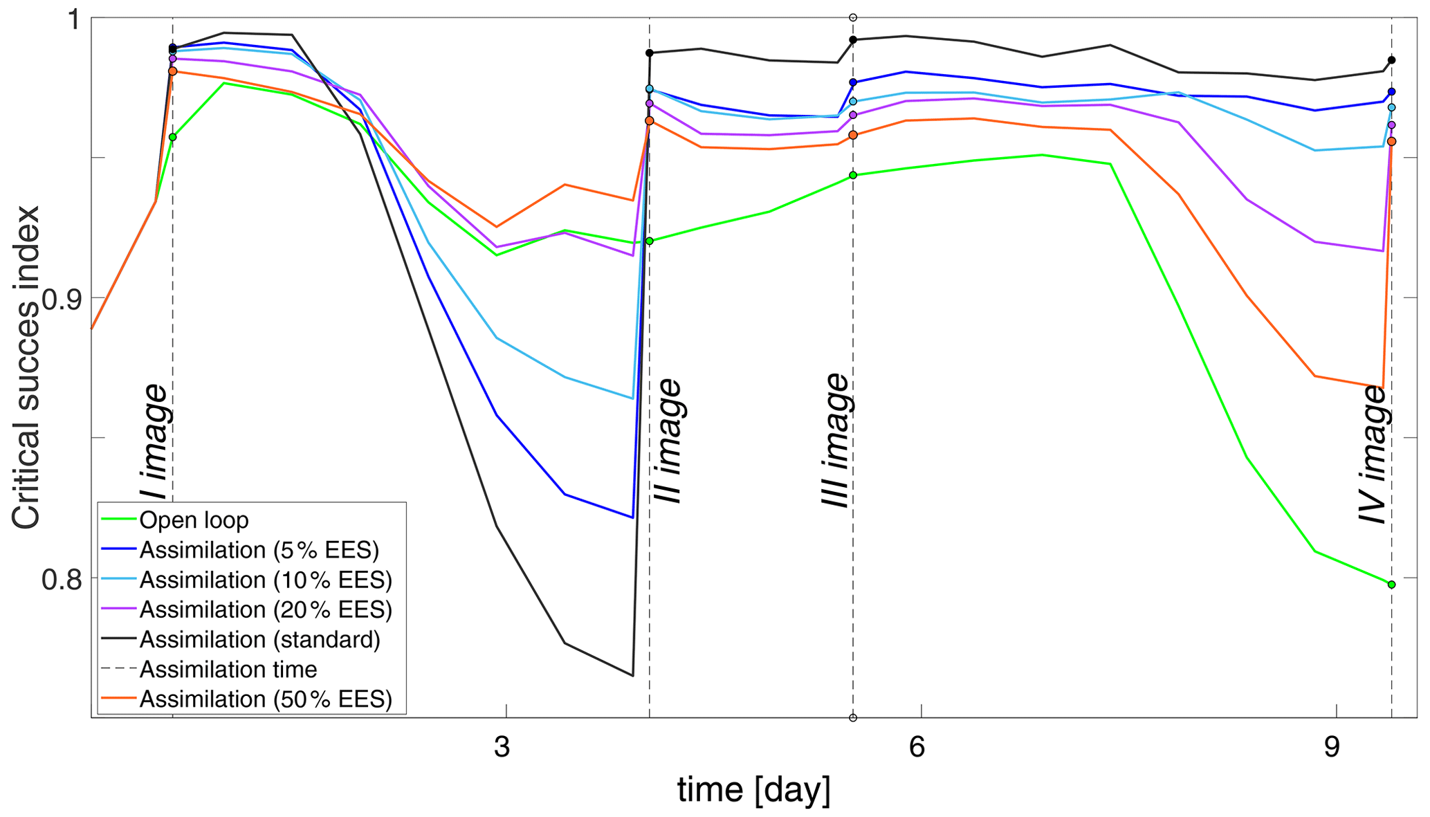
Figure 8 Time series of the CSI of flood extent values for the different assimilation methods: open loop (green), standard assimilation (black), assimilations with 5 % EES (blue), 10 % EES (cyan), 20 % EES (purple), and 50 % EES (orange).

This figure shows that the OL's performance is consistently poor and the standard assimilation performs best compared to the other assimilation runs at all the assimilation time steps.

The assimilation runs with different EES values lie within these two extremes. It can be noted that the more particles that are neglected, which is equivalent to saying the lower the EES, the higher is the performance at the assimilation time step.

Moreover, markedly different CSI time series for the different assimilation experiments are shown in Fig. 8.

After 27 h from the first assimilation, the performances of the standard and 5 % EES methods, which perform better than the other methods, start decreasing. The lowest values are reached 54 h after the assimilation. One explanation is that the weights assigned to the particles at the first assimilation time are no longer valid when hydraulic conditions change and need to be recomputed.

However, things change after the second assimilation, when the performances of the standard and the 5 % EES assimilation methods remain stable until the end of the simulation time.

The decrease in performance attributed to the standard and 5 % assimilation methods after the first time step is due to a drastic change in the flood extent. The total number of flooded pixels reduces from 8539 to 5494 because the flood started receding.

The spread of the posterior PDF with the standard and 5 % EES methods is small, meaning that only a few particles retain significant importance weight. Consequently, when the flood extent changes and particles evolve in time, it may happen that the uncertainty bounds of the posterior PDF do not encompass the true model state after several time steps. On the contrary, when more particles are considered (higher EES), more particles are used to draw the posterior PDF. This gives more chances for the ensemble to encompass the synthetic truth and increases the overall robustness of the method. This becomes particularly relevant when the hydraulic boundary conditions change and no new observation is available.

4.4 Evaluation of the water levels in time over a global scale

The RMSE, reported in Table 3 decreases by factors larger than 2 and 3 with the standard assimilation and the 5% EES assimilation, respectively. After the first assimilation, carried out close to the flood peak in Saxons Lode, the accuracy of the water level is improved by approximately 20 cm over the entire flood domain. The assimilation of the second and fourth images has a negative effect when the adapted method 50 % EES of the assimilation particle filter is applied; the RMSE increases compared to the OL. As already shown in Table 3, the standard assimilation and 5 % EES predictions of water levels provide more accurate results (Fig. 9). When moving away from the first assimilation, the RMSE of the best performing assimilation methods increases. For instance, after 54 h the RMSE of the standard method is increased by 65 % compared to the RMSE of the OL. When different values of EES are considered, the RMSE values fluctuates significantly in between two assimilations and it becomes difficult to draw any general conclusions. As the number of important particles increases, water levels vary significantly, especially in the area close to the flood edge even though the flood extent does not change too much from one particle to another.

Table 3 Root mean square error (RMSE [m]) at each assimilation time step. The open loop (Fig. 6) where no assimilation is computed is compared with the standard method and the adapted method with an increasing effective ensemble size (EES).

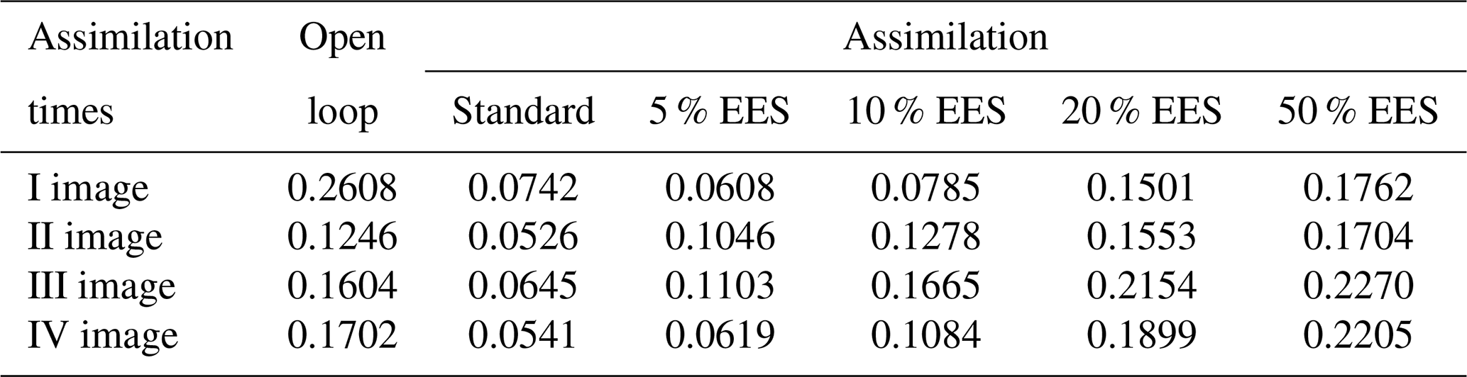
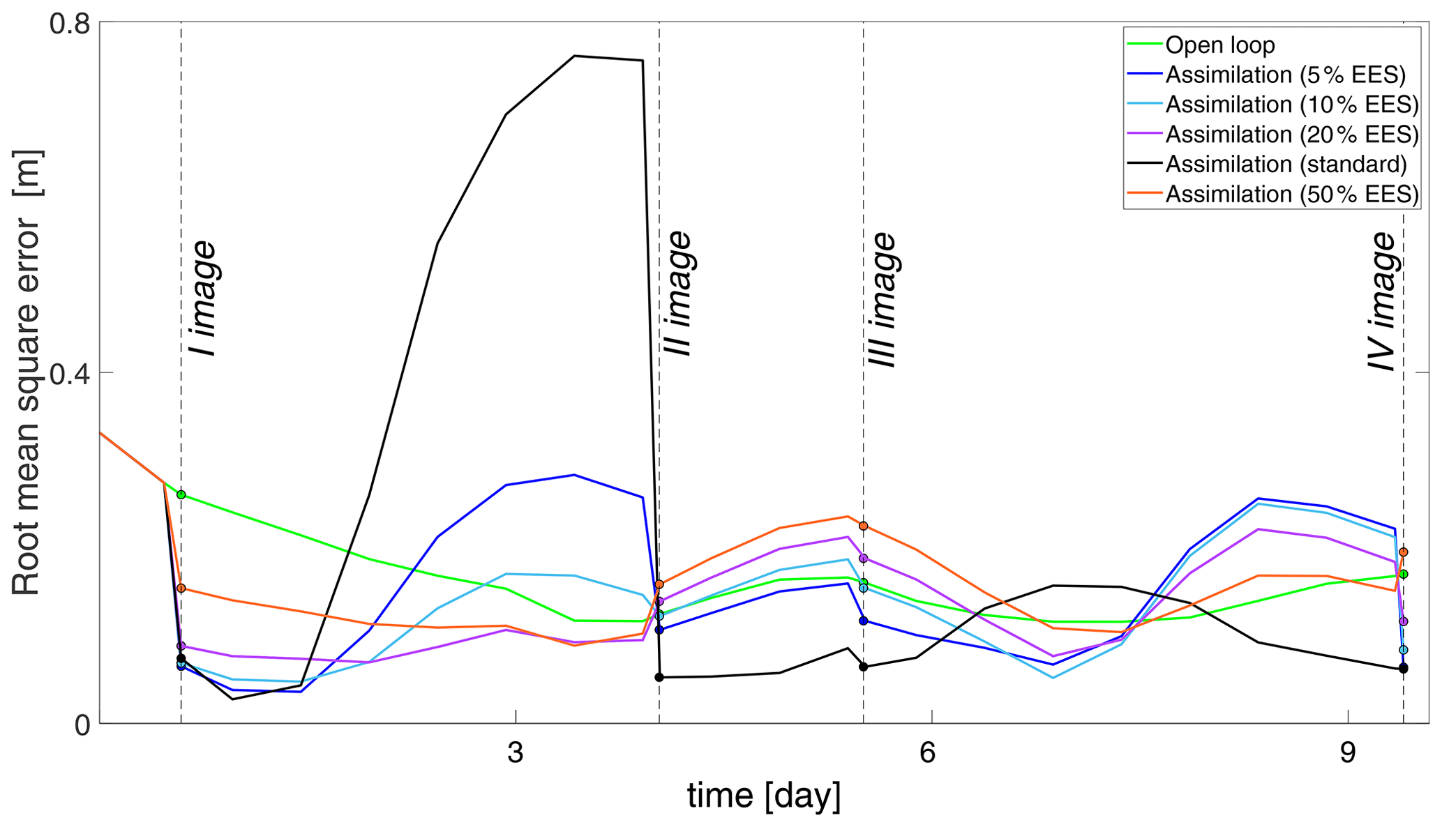
Figure 9 Time series of root mean square error (RMSE [m]) values for the different assimilation experiments: open loop (green), standard assimilation (black), assimilations with 5 % EES (blue), 10 % EES (cyan), 20 % EES (purple), and 50 % EES (orange).

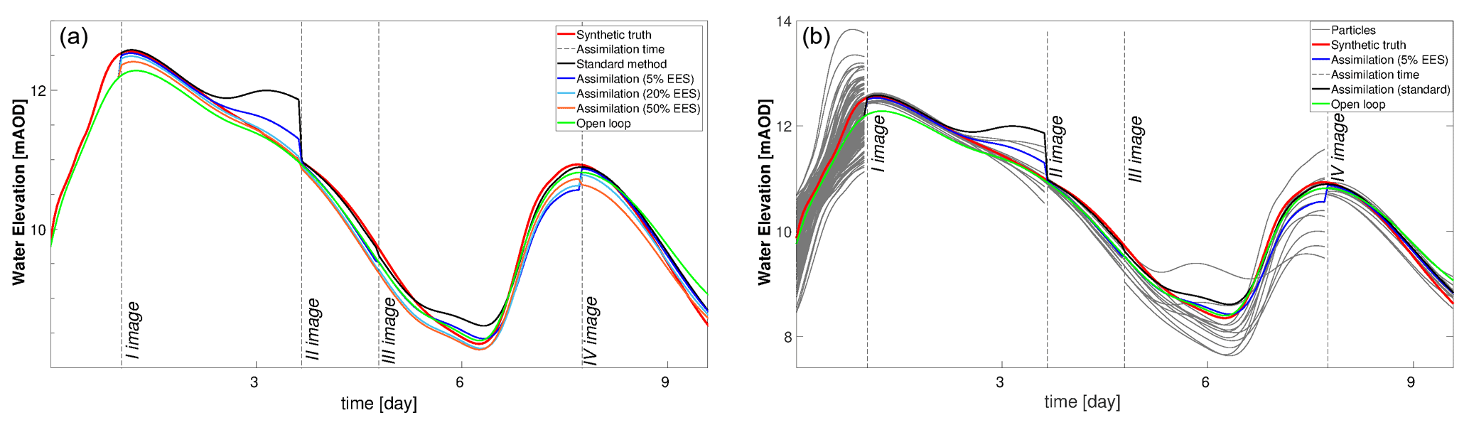
Figure 10 Water level time series at Saxons Lode. (a) Assimilation runs with an EES of 5 % (blue), 20 % (cyan), and 50 % (orange) as well as OL (green) and standard assimilation (black). (b) Particles carrying significant weight after the assimilation at 5 % EES (gray). Dashed lines correspond to the assimilation times.

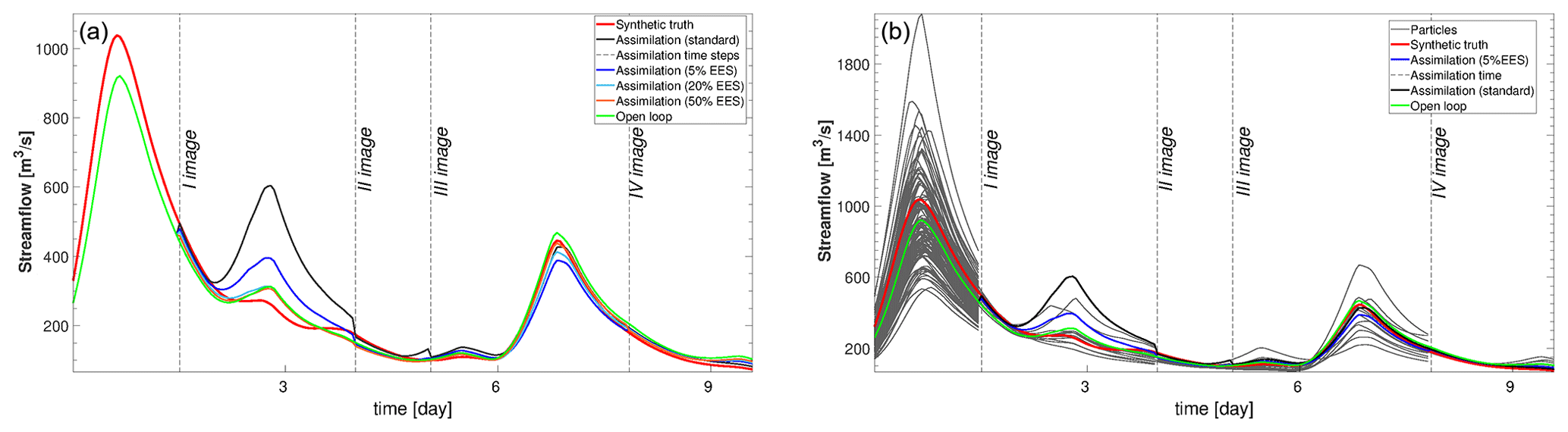
Figure 11 Streamflow time series at Bewdley. (a) Assimilation runs with an EES of 5 % (blue), 20 % (cyan), and 50 % (orange) as well as OL (green) and standard assimilation (black). (b) Particles carrying significant weight after the assimilation at 5 % EES (gray). Dashed lines correspond to the assimilation times.

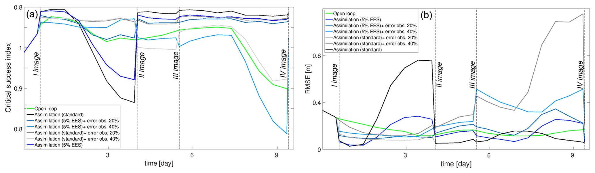
Figure 12 The CSI values (a) and RMSE (b) after the standard assimilation of SAR observations free of errors (black), with 20 % errors (gray), and with 40 % errors (light gray) as well as after the 5 % EES assimilation free of errors (blue), with 20 % errors (light blue), and with 40 % errors (cyan).

4.5 Evaluation of discharge and water level time series

The different assimilation runs are also compared considering the discharges and water levels at different gauge stations along the river Severn. In the right panels of Figs. 10 and 11 the different assimilation experiments are compared against the synthetic truth (red line). In the left panels of Figs. 10 and 11 the standard method and the 5 % EES assimilation with the important particles and the synthetic truth are shown. The plotted important particles represent 5 % of the ensemble with the largest weight. All 128 particles are equally weighted until the first observation is assimilated. After the first assimilation the number of important particles decreases. At the second assimilation time step, weights are recomputed and the new important particles are selected again and so on. The assimilation of the PFMs improves the predictions of water levels and streamflow at specific points of the river Severn, as in Bewdley and in Saxons Lode (Figs. 10 and 11), for the majority of the assimilation time steps in both underprediction and overprediction cases. The standard method and similarly the 5 % EES assimilation method are the most accurate in forecasting the values of water levels and streamflows. The improvements due to the assimilation persist for a long time: up to 27 h after the first assimilation predictions are still close to the synthetic truth. The local results of water levels suggest that the inaccuracy of the global RMSE values in time is likely due to the evaluation over the entire flood domain.

4.6 Impact assessment of errors in SAR observations

In the previous section, speckle uncertainty in SAR observations is considered. However, in reality, SAR observations are also susceptible to errors due to the misclassification of wet/dry pixels caused by features on the ground as already mentioned. Therefore, errors are added to the synthetic SAR observations as described in the methodology to investigate the impact on the DA assimilation framework. Figure 12 shows the RMSE and the CSI obtained at different assimilation time steps. The best performing assimilation methods (i.e., standard and 5 % EES) with no error in the observations are compared with those where error is introduced. With the misclassification of 20 % of the pixels, the assimilation still has beneficial effects: the CSI increases at each assimilation time step with respect to the OL. The RMSE values also tend to be satisfactory after each assimilation. With an increase in the error of 40 %, the performance of the DA framework starts decreasing. The assimilation of the first image still has a positive effect on the predictions. In fact, the CSI and RMSE are improved with respect to the OL even through the improvements are not as significant as in the previous cases. The explanation is arguably to be found in the high number of flooded pixels. It is large enough to counterbalance the misclassified pixels in the SAR image. Performance decreases with the assimilation of the remaining SAR observations when the number of flooded pixels is reduced by half.

5 Conclusions

Satellite images provide valuable information about flood extent that can complement or substitute in situ measurements. The fact that several space agencies provide free access to high-resolution satellite Earth observation data paves the way for improving Earth Observation-based flood forecasting and reanalyses worldwide. This study represents a follow-up of the previous real-world case study by Hostache et al. (2018) with the objective to further proceed in the evaluation of the proposed DA framework once the assumptions are effectively satisfied. This study has been set up in a controlled environment using a synthetically generated dataset in order to make sure that the rainfall and SAR observations are the only source of uncertainty. A common issue in particle filters is degeneracy: the ensemble could collapse after the assimilation because higher probabilities are assigned to a limited number of particles. The tempering coefficient can be used to reduce degeneracy because it inflates the posterior probability and reduces the peak of the likelihood. In this study, we have evaluated the effect of variations of the α tempering coefficient on the DA performance. Different PFs are compared with the OL and the synthetic truth: the SIS (with only a few particles from the ensemble potentially carrying non-negligible weights) and the adapted method with 5 %, 10 %, 20 %, and 50 % EES (with the number of particles with non-negligible weights increasing with the EES). This methodology leads to slightly biased estimates because the observation is down-weighted. In addition, we investigated the impact of errors in the observations (i.e., errors in the SAR derived PFMs due to dry water-lookalike pixels or emerging objects) on the assimilation. Indeed, the main issue of using SAR observations in flood forecasting models is the difficulty of detecting the flooded area for specific cases (e.g., urban or vegetated areas). At first, following the study from Hostache et al. (2018), only speckle uncertainty of the SAR image is taken into account in the PFMs. In a second step, an error to reproduce misclassified pixels is introduced in the synthetic SAR observations.

The following key conclusions can be drawn from our experiments:

1. The best performing method is the standard method (i.e., SIS). Importance weights are assigned to a limited number of particles that better agree with the observations. At the time of the assimilation, results tend to be very accurate: the forecasts move close to the synthetic truth. The main weakness of the standard filter is that it significantly suffers from degeneracy.

2. The 5 % effective ensemble size assimilation (meaning that only the 5 % of the ensemble will have a non-negligible weight after the assimilation) is slightly less accurate at the time of the assimilation but it has the advantage of reducing the degeneracy problem. Even though a larger effective ensemble size prevents degeneracy, the results are less accurate and the performance of the predictions are degraded.

3. Our study further shows that it is important to characterize and mask out errors in the SAR observations. A large number of misclassified pixels substantially degrades the DA performance. In our case study, results suggest that an improvement of model simulations (i.e., water level and streamflow) in terms of the CSI and RMSE performance metrics is achieved as long as errors in the observations are rather limited, i.e., when no more than 20 % of the pixels are affected. However, if the misclassification goes beyond 40 % of the affected pixels, the assimilation has no effect and may even lead to a degradation of the model predictions.

6 Discussion

The results of our study confirm the effectiveness of the proposed DA framework when the hypothesis of the rainfall as the main source of uncertainty is verified. Consequently, for those cases where rainfall represents the main source of uncertainty, more obviously but not only in poorly and un-gauged catchments and when using medium-range forecasting models, our study results indicate that the application of the approach described in this paper may lead to improved results of the model simulations. For those cases where the uncertainty of other sources becomes more relevant and may even be dominant, it is clear that such sources need to be taken into account explicitly. However, the required adaptations of the proposed DA framework still need to be developed. In this context it is also worth mentioning that the limitations identified in the previously published real-world case study by Hostache et al. (2018) were explained by additional sources of uncertainties not taken into account.

Using probabilistic flood maps or backscatter values increases the number of observations to be assimilated when compared to a method that only derives the flood edge from satellite observations as reported in Cooper et al. (2018). Moreover, the nearly direct use of the SAR information enables faster end-to-end processing from the acquisition of the image to the assimilation of the SAR data into the model, which is beneficial for operational usage.

In our experiments, the improvements of model forecasts of water level and streamflow are significant at the assimilation time step and the improvements persist over subsequent time steps (for example up to 27 h after the first assimilation the model results outperform the open loop simulation). The persistence of these improvements depends on the flashiness of the flood event (i.e., the rapidity with which hydrologic conditions change). More frequent image acquisitions could help keep model predictions on track, especially when the system is highly dynamic. The update of a state variable of the forecasting model could as well increase the persistence of the improvements. In our study none of the model state variables is updated as only the particle weights are computed, based on the SAR observations and on the simulated flood extent maps, and used to calculate the expectation of water levels and streamflow. In previous studies (Andreadis et al., 2007; Matgen et al., 2010; Cooper et al., 2019), inflow updating was identified as a condition leading to more persistent improvements. For instance, one of the conclusions from the study by Matgen et al. (2010) was that updating the fluxes at the upstream boundary conditions, rather than the water levels, is more effective because of the high uncertainty of the inflow due to the poorly known rainfall distribution over the catchment. Therefore, as a future perspective, we aim to update hydrologic model states because it might have a positive impact on the long-term runoff simulations and consequently on the persistence of DA benefits.

Some modifications of the DA framework are still required to fully overcome the issue of degeneracy. Although the use of a smaller tempering coefficient leads to a larger effective ensemble size (e.g., 50 %) and helps avoid degeneracy, the results are less accurate compared to the standard method or the adapted method with 5 % EES. As described in Neal (1996) and in van Leeuwen et al. (2019), the tempering procedure consists of several steps, but in this study the tempering coefficient is applied only to flatten the likelihood, therefore down-weighting the observations. This most likely explains why the data assimilation performs better when the effective ensemble size (the number of non-negligible particles after the assimilation) is smaller. As already mentioned, the present study has the aim of assessing and validating the method proposed by Hostache et al. (2018) in a synthetic environment. Our DA framework can be applied to a variety of flood inundation forecasting chains. In fact, the forecast updating is carried out via sequential importance sampling only (i.e., importance weights). Only the particle weights are updated based on the observations and used to compute the expectation (i.e., weighted mean) of the augmented state vector including hydraulic state variables of water depth plus the flood extent and boundary conditions. In this study, the hydrologic and hydraulic models are loosely coupled with a one-way transfer of information as in many other studies (e.g., Peckham et al., 2013; Hoch et al., 2017; Rajib et al., 2020). The weights define the relative importance of the particles and thus of the inherent streamflow and stage along the entire river. We acknowledge that the observed flood extent is more closely linked to the past boundary conditions rather than the boundary conditions corresponding to the assimilation time steps. In spite of this limitation we argue that in this synthetic experiment, the particles that performed best in the past are also those that reach the highest performance level at the time of the assimilation. This is illustrated in Figs. 10 and 11 where the use of updated weights is shown to enable the correction of the state variables of the hydraulic model both upstream and downstream. However, we recognize that further improvements could be developed to address issues such as spurious relations that may occur between SAR observations and model variables due to a rather small ensemble size. Enlarging the ensemble size could be necessary if this occurs.

We also argue that the method used in this paper has the potential to support EO-based modeling at large scale. This potential is particularly high in large, natural floodplains where flood inundation remains present over long time periods. In spite of the increased frequency of satellite observations, the persistence of a flood over many days increases the chance of its detection and mapping by satellite sensors. Another condition that needs to be satisfied is that there should be an unambiguous relationship between the flood extent observed by the spaceborne sensors and river discharge. This also means that areas where backscatter variations are not impacted by the appearance of floodwater (e.g., densely vegetated floodplains) should be rather small. Indeed, these constraints must be satisfied to enable a successful application of the proposed framework and to take advantage of the analysis carried out in this paper. Based on the above elements, we argue that our approach is valid regardless of the type of model coupling that is performed and is thus applicable to many different forecasting systems. However, more research is needed to fully understand the role of floodplain and water basin characteristics and SAR data properties on the DA performance. In a future study it is envisaged that to avoid degeneracy and keep a larger effective ensemble size, the full tempering scheme will be applied. Possible ways to adapt and advance the proposed DA framework are currently under development (e.g., updating a state variable of the model and using an enhanced version of the adapted filter).