Technical note: Hydrology modelling R packages – a unified analysis of models and practicalities from a user perspective

Following the rise of R as a scientific programming language, the increasing requirement for more transferable research and the growth of data availability in hydrology, R packages containing hydrological models are becoming more and more available as an open-source resource to hydrologists. Corresponding to the core of the hydrological studies workflow, their value is increasingly meaningful regarding the reliability of methods and results. Despite package and model distinctiveness, no study has ever provided a comparison of R packages for conceptual rainfall–runoff modelling from a user perspective by contrasting their philosophy, model characteristics and ease of use. We have selected eight packages based on our ability to consistently run their models on simple hydrology modelling examples. We have uniformly analysed the exact structure of seven of the hydrological models integrated into these R packages in terms of conceptual storages and fluxes, spatial discretisation, data requirements and output provided. The analysis showed that very different modelling choices are associated with these packages, which emphasises various hydrological concepts. These specificities are not always sufficiently well explained by the package documentation. Therefore a synthesis of the package functionalities was performed from a user perspective. This synthesis helps to inform the selection of which packages could/should be used depending on the problem at hand. In this regard, the technical features, documentation, R implementations and computational times were investigated. Moreover, by providing a framework for package comparison, this study is a step forward towards supporting more transferable and reusable methods and results for hydrological modelling in R.

1 Introduction

Since the early 1960s, many hydrologists have been designing models to better understand water cycle processes controlling river flows (e.g. Todini, 2011; Beven, 2012). These models have enabled advances with respect to a wide variety of applications in hydrology, such as flood forecasting, climate change impact assessment and water resources management. The processes involved in the motion of water at the catchment scale are complex (e.g. Wagener et al., 2010), mainly due to the heterogeneity and nonlinearity of the physical properties involved. Hydrological modelling can, therefore, be of great use regarding many scientific challenges, as it relies on a threefold simplification of time, space and hydrological processes to either match the average behaviour of the water cycle (Singh et al., 2017) or focus on flow extremes (e.g. floods, Georgakakos, 2006, and Rozalis et al., 2010, or low flows, Staudinger et al., 2011, and Nicolle et al., 2014).

Various types of hydrological models exist, which differ according to their assumptions on the representation of natural processes and space and time dependencies (e.g. Clark et al., 2011, 2017; Beven, 2012). Various programming languages enable the use of these hydrological models. For example, some models are implemented in Python (e.g. EXP-HYDRO hydrological model; Patil and Stieglitz, 2014) or in MATLAB with the MARRMoT toolbox (Knoben et al., 2019). A significant number of models like MIKE SHE (Danish Hydraulic Institute, 2017) can only be operated through commercial software and platforms.

A large number of models can be found on the R platform. The R language (R Core Team, 2020a) is an open-source interpreted language. It was originally designed for statistics (as an open-source implementation of the S language; Becker et al., 1988) but has since been employed in many other scientific fields. The functionalities of the R language can be extended by packages, some of which include features related to hydrology topics. There is a growing community of users and a large range of documentation, tutorials, manuals and online discussion platforms that have been developed by the R-Hydro community, such as the CRAN Hydrology Task View on hydrological data and modelling (https://cran.r-project.org/web/views/Hydrology.html, last access: 1 March 2021) or the page related to R on the AboutHydrology blog (https://abouthydrology.blogspot.com, last access: 1 March 2021). In addition, many short courses and workshops are regularly organised (e.g. the “Using R in Hydrology” short course at the European Geosciences Union (EGU) General Assembly). The R-Hydro community is also very active in many R projects and websites, such as the rOpenSci project (https://ropensci.org, last access: 1 March 2021) or the many code examples available on Stack Overflow (https://stackoverflow.com, last access: 1 March 2021). R can be used at each step required for a basic study in hydrology (the hydrological workflow steps, see Fig. 3 of Slater et al., 2019, that shows the growth of available packages over the last 10 years). Consequently, there has been an important increase in the growth and use of hydrological R packages (see Fig. 1 of Slater et al., 2019). Some of these packages are designed for hydrological modelling. In this study, we will restrict ourselves to the hydrological models that are available within the R environment.

At a time when data management is a key issue in many branches of science, R has taken a central place in hydrology (Slater et al., 2019). Dealing with the rise of available data can be achieved within the R environment through the numerous packages for data preprocessing, such as rnrfa (Vitolo et al., 2016a, 2018), used to retrieve hydrological data from the UK National River Flow Archive, or raster (Hijmans, 2020) to manipulate spatial data. While this growing availability of open-source data and methods is concomitant with the increasing development of open-source models, there has never been any comparison of hydrological modelling R packages. Such a comparison is required to improve the usability of hydrological models included in the R environment. Comparison is a step towards overcoming reproducibility issues related to modelling in computational hydrology (Ceola et al., 2015; Hutton et al., 2016; Melsen et al., 2017). Furthermore, in addition to the struggle associated with a large number of hydrological models and the difficulty in finding appropriate bases for model selection (Clark et al., 2011; Beven, 2012), there are many R packages related to hydrological modelling, making it even harder to select the model best suited for a specific case. Catching the modelling philosophy (Hrachowitz and Clark, 2017) or differences in a perceptual model (Wrede et al., 2015) behind the packages, as well as the technical features offered by a package, therefore appears to be relevant to hydrologists, whether it aims at improving the reliability of intercomparisons or simply at correctly selecting a model. By referring to the provided documentation, any user should be able to make a choice and use a model in full knowledge of its characteristics, thus guaranteeing good practices (Jakeman et al., 2006). Unfortunately, despite the wish to standardise package documentation, especially regarding the rules imposed by the main R packages repository, the Comprehensive R Archive Network (CRAN; https://cran.r-project.org/, last access: 1 March 2021), it remains complicated and sometimes even daunting to select a package among the R packages containing hydrological models. Yet, to our knowledge, there has never been a published study dealing with the comparison of hydrological modelling R packages. This work should (i) enable any newcomer in hydrology, or even more experienced hydrologist, to knowledgeably employ one of the packages presented in this comparison and (ii) highlight possible improvements for future developments of the packages.

The review paper published in the Hydrology and Earth System Sciences journal by Slater et al. (2019) on the place of R in Hydrology has reached a large part of the hydrological science community. Our work follows on from this review and aims at reaching a large portion of hydrological modellers within the R-Hydro community, from beginners to highly skilled developers. The objective of this paper is to review the pros and cons of using hydrological models implemented within packages in the R environment and to compare and evaluate their applicability and usability. It is not the intention to describe new hydrological model developments or evaluate the models. We present the package selection rationale and the comparison methodology in Sect. 2. We provide an overview of each package with their related models in Sect. 3. We examine these models in terms of implied conceptual storages and fluxes, spatial discretisation, model requirements and outputs in Sect. 4. The hydrological model packages are evaluated according to their functionalities, provided documentation, R implementation and computational efficiency in Sect. 5. We discuss the usefulness of our analysis, possible improvements for future developments and aspects of practical implementation in Sect. 6. Simple hydrology modelling examples are provided in the form of R source code.

2 Methodology

There is a wide variety of models contained in the R packages that we have selected for this study. To lay the foundations of our analysis, we first present in this section how we have selected the packages, then we introduce the framework for analysing the models and the packages from a user perspective. Here we make a distinction between R packages and the hydrological models that are implemented within the packages. In this framework for analysis, we separate model conceptualisation (Sect. 2.2) from package practicalities (Sect. 2.3). The model conceptualisation is analysed in terms of model structure (Sect. 2.2.1), how to break up a catchment (Sect. 2.2.2) and the number of parameters, time steps, inputs and outputs required (Sect. 2.2.3). The package practicalities are analysed in terms of functionalities (Sect. 2.3.1) and usability (Sect. 2.3.2, 2.3.3 and 2.3.4).

2.1 Selection of packages

Deciding upon the number of packages implies finding the right balance between including many packages and conducting a thorough assessment. On the one hand, our aim was to select as many packages as possible in order to present an extensive comparison. On the other hand, to allow a comparison, only models with similar set-ups could be used; thus, we had to narrow our list to do so. In this regard, we have selected the packages containing conceptual (bucket-type) continuous rainfall–runoff models as they were the most frequently encountered during our search and are widely used for many applications in hydrology (e.g. Shin and Kim, 2016). Furthermore, compared to more complex physical models, conceptual models usually have lower data requirements (e.g. Clark et al., 2017; Knoben et al., 2019) and a smaller computational demand. This makes it easier for users to employ the models.

We based our search on the following four sources: the CRAN, GitHub (https://github.com/, last access: 20 September 2020), the R-Forge (https://r-forge.r-project.org/, last access: 20 September 2020) and a CRAN Task View dedicated to hydrology. GitHub is a development platform based on the Git version control software. The R-Forge is a development platform specific for R packages. It is based on the Subversion version control software and offers tools, such as automatic build and checking of packages or mailing lists and forums. Task Views are guides – proposed by the CRAN – on the main packages related to a certain topic. Many R packages are stored on the CRAN that contains more than 15 000 packages. Many other packages (around 1500) are only available on GitHub and some packages are stored on the R-Forge. Some of the packages stored on the CRAN are also available on GitHub or on the R-Forge. Among these packages, some were designed for hydrological purposes. To identify as many packages as possible, we searched for packages on the CRAN, GitHub and the R-Forge by using keywords. Among the CRAN Task Views, we used the work of Zipper et al. (2019), who established a list sorting the hydrology-related packages by topics (data retrieval, statistical modelling, etc.). We looked at the packages considered as being aimed at modelling (process-based modelling category) in this Hydrology Task View. The review paper by Slater et al. (2019) about the place of R in hydrology includes a section related to hydrological modelling in which some of the packages compared in our study are briefly introduced. Despite our intention to create an exhaustive list, we might have missed some packages due to the different organisation of repositories such as GitHub and the R-Forge compared to the CRAN.

2.2 Framework for analysing the hydrological models

Investigating the different hydrological characteristics behind the models contained in the R packages is a difficult but useful exercise. It aims at gathering information about the various hydrological visions available in a comparative framework. It is relevant to proceed with this comparison task to help any student or more experienced hydrologist to understand what is involved when using a specific model implemented in one of the R packages. The selected packages contain various hydrological models based on different assumptions. These assumptions can be sorted out into simplification options regarding storages, fluxes, time and space. In this comparative study, we first propose a unified comparison of the conceptual representation of storages and fluxes by the models included in the selected packages, then the spatial discretisation they imply and, finally, a description of model requirements and retrievable outputs via the packages. The unified representations should allow more consistent comparisons and, therefore, help the modellers in their choice of methodology for a specific case study. Package documentation and source codes were thoroughly screened to conduct these analyses. This work was carried out in accordance with the comments and recommendations of most of the package authors.

2.2.1 Conceptual representation of storages and fluxes

Each model has its own degree of complexity regarding the representation of storages and fluxes. The differences in model structure partly depend on the perceptual model of how a catchment is functioning (e.g. Wrede et al., 2015). In our list of seven models, these differences resulted in very different modelling characteristics. One of the goals here is to present the exact modelling structure contained in the selected packages. The reader has to be aware that these might have been adjusted from the original versions by the package authors. We have, therefore, adopted a comparison method that aims at representing the main principles behind the models – or differences in a perceptual model – but that still keeps a certain degree of precision. This type of unified comparison was, for example, employed in the framework for understanding structural errors (FUSE; see Fig. 3 of Clark et al., 2008) to compare the structures of four models or to present the 40 models included in the MarRMOT toolbox (see Fig. 2 of Knoben et al., 2019).

We selected an approach for this analysis that derives from the work of de Boer-Euser et al. (2017, Fig. 3). This analysis aims at depicting the conceptual storages and fluxes at a spatial unit scale. More details about the diagrams are given in Sect. 4.1 and Fig. 1. This analysis was reviewed by the package authors to ensure consistency.

2.2.2 Spatial distribution

Users must be aware of the spatial discretisation that is available. Furthermore, some packages offer the possibility to apply different types of catchment discretisations for the same model. We, therefore, present the different cases for the selected packages after introducing a special case that is snow modelling spatial distribution.

2.2.3 Requirements and outputs

Since hydrological models do not always rely on the same assumptions, their requirements, i.e. data inputs and number of adjustable parameters, can differ. As data availability can sometimes be a restraining factor, it is essential for users to be informed about the model data requirements. The packages also allow the operation of the models at different time steps and imply different types of numerical resolutions of model equations. The different equations of a hydrological model can be solved using different techniques. The equations are solved analytically (the exact solution is determined by integrating the equation for a given time step), explicitly (the solution is approximated by its derivative at the beginning of the time step) or implicitly (the solution is approximated by its derivative at the end of the time step). When the solution is analytical or explicit, the operator splitting technique (OS) is commonly applied to solve the model equations. When OS is applied, the different processes, such as evaporation, runoff and percolation are calculated sequentially (Santos et al., 2018b). Numerical solution in hydrology can be seen as part of the mathematical model structure rather than software implementation, as it changes the results substantially (Clark and Kavetski, 2010; Kavetski and Clark, 2010).

By making different outputs available, R packages allow modellers to better assess the suitability of applying a model for a specific problem. It can also facilitate the evaluation of appropriate parameter estimation, i.e finding a consistent set of parameters. Among the practical outputs for a modeller, time series of actual evapotranspiration estimates can be useful for understanding the behaviour of the soil moisture accounting functions. Retrieving time series of runoff components (e.g. fast runoff and very quick runoff), which are highlighted by Sect. 4.1, makes it possible to relate the model simulations with catchment regimes (e.g. high baseflow well reproduced by the slow runoff exiting the groundwater store). Internal fluxes can inform a user on the internal consistency of a simulation, for example, to identify the fraction of effective rainfall exiting the root zone store and reaching the fast runoff routine compared to the fraction entering the groundwater store. Analysing time series of store levels can, for instance, enlighten the user on whether the root zone store capacity has been correctly estimated, which would then help to analyse the simulation of soil moisture seasonality by the model for the studied catchment.

Any modeller would need to understand these specificities in order to select and apply a model. We summarise these characteristics (requirements, time step and numerical resolution and outputs) in Sect. 4.3.

2.3 Framework for analysing package practicalities

The different packages implement a set of functionalities to operate the models, which can be more or less in line with the hydrological workflow, i.e. from data preparation to analysis of the results. These functionalities aim at easing and sometimes constraining the use of the model. One would expect to use all the functionalities required to consistently apply a specific model and avoid any supplementary source of errors. One of the specificities of R packages is the provided documentation. The related description and examples must be complete to ensure the appropriate application of the models. The user is guided by basic examples and is made aware of potential errors that can occur. Following the analysis of functionalities and documentation, we present an analysis of R implementation that should foster more rigorous applications of the models. In an effort to contribute to more extensive documentation relating to the packages and their models, we provide R scripts enabling the use of each package on simple examples. A short analysis of central processing unit (CPU) times is derived from the application of these scripts.

2.3.1 Functionalities

What a package provides in terms of functionalities is a distinguishing feature when selecting a specific software or another programming language for hydrological modelling. Among the main features, we usually find the careful preparation of input data to respect the right time references, initialisation period or specific R objects. Enabling an automatic calibration procedure to find a set of parameters consistent with the catchment of study can be an important step for some models as well (though some packages have specifically avoided automatic calibration for the reasons discussed in Beven, 2012, 2016). Functions that allow the users to visualise and analyse the results are often appreciated. Simple analyses can be the calculation of criteria assessing the overall performance, for example. These criteria are regularly calculated on time series of transformed data to emphasise specific error characteristics. Hydrograph plots are also common for assessing hydrological models. Graphical user interfaces can increase the package usability. As some models enable snow calculations, implementing an independent snow function is necessary to avoid using a snow function on non-snowy catchments. One of the advantages of working within the R framework is that the code can often be modified by the user to access more variables or to calculate additional performance measures, etc., although some of the packages also include compiled components that might make this more difficult.

We present in this analysis whether the selected packages integrate these basic functionalities to consistently apply the models. Inspections of the packages were conducted based on the different types of documents related to the packages and models. When judged necessary, the codes were analysed to ensure accurate results.

2.3.2 Documentation

To handle the complexity associated with the different hydrological models and with the functionalities provided by the packages, the documentation is obviously essential for any user. It is, therefore, important to assess whether looking at the overall documentation is sufficient to easily make use of the package basics. In this regard, we compared the available explanatory documents. This analysis is, by definition, subjective as it relies on our experience as users. However, we think that it can still give insights into the meaningful content of the documentation. Analysing the documentation explanation by explanation would indeed be very complicated to present. There are the following two different types of documentation related to these packages: the R documentation that includes user manuals (functions explanations and mandatory for packages accepted by CRAN) and sometimes vignettes (“long-form guides that illustrate how to use packages”; Slater et al., 2019) and the external documentation that comprise scientific journal articles and sometimes websites. For each function of a package, the formal R user manual includes mandatory fields (e.g. name, value, title, description and arguments) and optional fields (e.g. details, examples and references; for more details see R Core Team, 2020b). We consider the following two types of scientific articles in this analysis: articles written to present the packages and articles using the packages and made by one of the package authors. Websites usually contain elements such as video tutorials, a list of publications mentioning the package, examples and user groups. Vignettes and external documentation are not required when creating a package but can be very useful for a thorough understanding of the packages and models.

2.3.3 User implementation

Package practicalities can also be assessed through an analysis of the links between the main functions of a package. Such an examination could be useful to provide guidance regarding package application. We try to put ourselves in the shoes of users who have to apply the models of the different packages and, therefore, need to understand which function they have to use, where to use it in the script and how to use it. In this regard, we propose a unified diagram of the connections between the main functions that we have been able to run (see Fig. 4). We use the term user function, which means that users have to write their own R function integrating, among others, the legacies illustrated on the diagrams. This analysis is intended for users familiar with R packages and aims at guiding users in their application of the hydrological modelling R packages. We, therefore, provide R scripts enabling the application of each package on a simple hydrology example (Astagneau et al., 2020). The provided R scripts show the basic R commands required to test one parameter set on two different catchments (see Sect. 2.3.4).

2.3.4 R structures and CPU times

Package developers made several choices in terms of R implementation that can affect package usability. For that reason, we analyse the programming languages and external dependencies. We also perform a short analysis of package CPU times.

Some packages are entirely coded in R, which is an interpreted language, and some integrate models coded with a compiled programming language interfaced with R. The different programming languages interfaced with R were identified by extracting the package sources because they could not necessarily be identified by simply displaying the code from the R console. We considered a package as dependent on external dependencies if one of its functions cannot be run without downloading another package. A package is not considered as being dependent on any other package when the use of an external package is only suggested in an example or in one of the related articles. Base packages, such as stats, and recommended packages (https://cran.r-project.org/src/contrib/3.6.0/Recommended, last access: 10 June 2021), such as lattice, are not taken into account in this assessment, as they are packages installed by default.

From a user perspective, computation times can be meaningful to determine whether a package is suitable for a specific study. Short computation times are usually very well appreciated, especially when dealing with finer time steps or more complex spatial discretisations. Applying a model to a large database, generating an ensemble in operational (flood) forecasting or performing Monte Carlo runs for uncertainty analyses can also significantly increase computation times; hence, some of the packages include some compiled code to speed up the production runs of the model. We analysed the CPU time required for one model run, which was estimated from 1000 runs with the microbenchmark package (Mersmann, 2019). We ran the packages on a computer with the following characteristics: random access memory (RAM) capacity – 8.00 GB; central processing unit (CPU) – Intel i5-8250U 1.80 GHz; operating system (OS) – Windows 10 (64 bit), using the 3.6.0 (64 bit) R version. The models were run at a daily time step on a catchment where high flows mostly result from precipitation events in winter, i.e. the Meuse River at Saint-Mihiel (2543 km²; from 1 January 1990 to 31 December 1999) and, for the packages integrating a snow function, on a mountainous catchment where high flows mostly result from snowmelt in spring, i.e. the Ubaye River at Lauzet-Ubaye (943 km²; from 1 January 1989 to 31 December 1998). The time series of precipitation and temperature at a daily time step were extracted by Delaigue et al. (2020b) from the SAFRAN countrywide climate reanalysis of Météo-France (Vidal et al., 2010). The potential evapotranspiration (PET) time series were calculated using the Oudin et al. (2005) formula. The streamflow data were retrieved from the “Banque Hydro” database (Leleu et al., 2014). For the use of some packages, a digital elevation model (DEM) with a resolution of 25 m by 25 m was derived from the BD ALTI DEM (IGN, 2013). Only one parameter set is tested for each model.

3 An overview of the selected hydrological modelling R packages

The outcome of our selection is a list of eight packages that will be carefully compared throughout the paper. Here we give a first overview of these packages along with their related bucket-type hydrological models. The full list is presented in Table 1 with the main related documentation. Table 2 shows the snow models contained in the selected packages.

Mouelhi (2003)Mouelhi et al. (2006)Perrin et al. (2003)Le Moine (2008)Pushpalatha et al. (2011)Mathevet (2005)Ficchì et al. (2019)Beven and Freer (2001)Metcalfe et al. (2015)Bergström (1976)Bergström and Lindström (2015)Croke and Jakeman (2004)Jakeman and Hornberger (1993)Boughton (2004)Perrin et al. (2003)Burnash (1995)Burnash (1995)Beven and Kirby (1979)Beven et al. (1995)Parajka et al. (2007)Brauer et al. (2014a)Brauer et al. (2014b)

Table 1 A list of the selected packages with their related models. The models included in the following analyses are in bold. The models included in hydromad that are presented in this table only correspond to the main soil moisture accounting functions (for more details, see Andrews and Guillaume, 2018).

Valéry et al. (2014)Bergström and Lindström (2015)Andrews and Guillaume (2018)Anderson (2006)Parajka et al. (2007)Seibert (1997)Kustas et al. (1994)

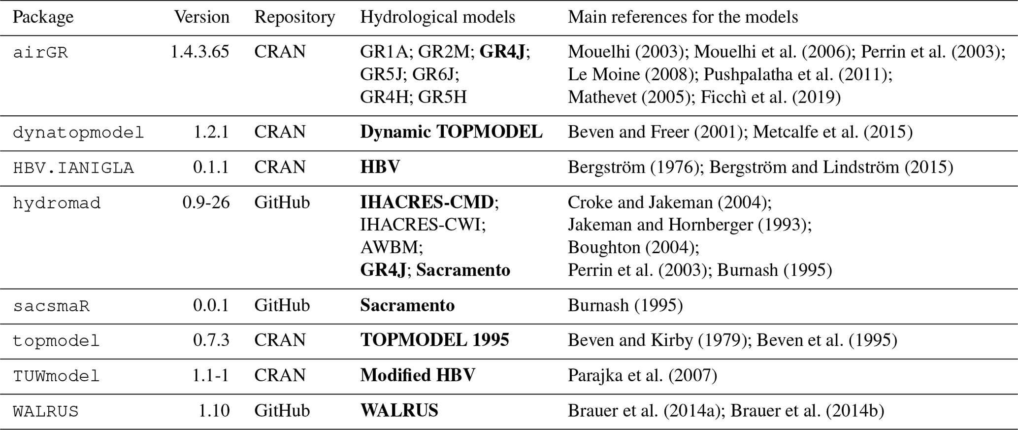
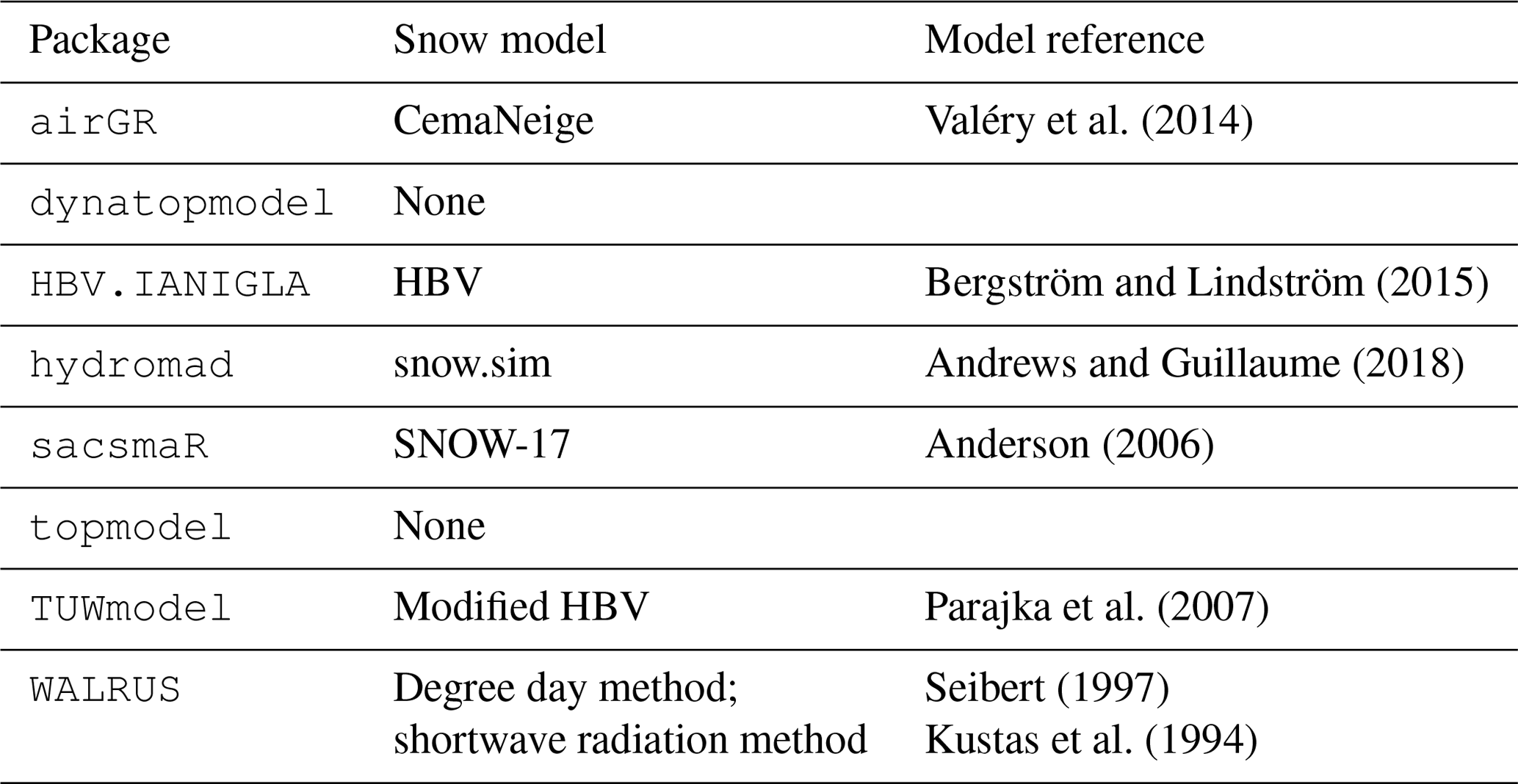
Table 2 A list of the snow models contained in the selected packages.

We chose to exclude the following packages, and we justify our choice in the following:

• The Ecohydmod package (Souza, 2017) implements an ecohydrological model.

• The LWF-BROOK90 package (Schmidt-Walter et al., 2020) implements a physically based land–surface hydrological model.

• The fuse package (Vitolo et al., 2016b) proposes a large number of model structure configurations. It was considered that its main purpose was not to conduct a basic hydrological study but more to understand errors arising from hydrological models. It is also in need of active maintenance.

• The RHMS package (Arabzadeh and Araghinejad, 2019) implements several event-based hydrological models. This package is not included in this work as we chose to include only the continuous models.

• The SWATmodel package (Fuka et al., 2014) implements a complex watershed hydrological transport model. This package does not provide any function for data preparation or any explanatory document.

airGR

The airGR package (Coron et al., 2020) implements the models constituting the suite of Génie rural (GR) hydrological models (Coron et al., 2017) originating in the work of Claude Michel, which started in the 1970s (Michel, 1983). These models are parsimonious conceptual rainfall–runoff models that consider a catchment as a single entity (lumped). Several versions were developed over the years, from the well-known GR4J (Perrin et al., 2003) to the GR6J model (Pushpalatha et al., 2011), for improved low-flow simulations. A snow accounting model called CemaNeige (Valéry et al., 2014) can be combined with the daily and hourly GR models or can also be operated independently. airGR includes a function to calculate potential evapotranspiration time series with the equation of Oudin et al. (2005). Various technical features associated with the hydrological workflow, from data preprocessing work to result analysis, are offered. For the sake of brevity, only GR4J combined with CemaNeige will be assessed in the following analyses. airGR has a graphical user interface in the complementary package airGRteaching (Delaigue et al., 2018, 2020a), which will be analysed along with airGR.

topmodel

The topography-based hydrological model (TOPMODEL; Beven and Kirby, 1979) has been employed for a variety of applications since its introduction (Beven et al., 2021). The TOPMODEL version included in topmodel (Buytaert, 2018) follows the version developed by Beven et al. (1995) that makes explicit assumptions about the nature of the near-surface water table responses that lead to the possibility of using a topographic wetness index (TWI) as an index of hydrological similarity to calculate surface saturation and moisture deficits. Calculations are made for different increments of the distribution of the index, making the model computationally fast to run. The pattern of the index can be derived from an analysis of a DEM and can be used to map the simulated response back into the space of the catchment. topmodel allows simple calculations from a DEM and basic data series required in conceptual hydrological modelling. TOPMODEL allows for saturated contributing areas to be predicted based on the spatial distribution of the topographic index. These assumptions mean that it is best suited to moderately sloping hillslopes with relatively shallow water tables (see Quinn et al., 1991, for an application to a deeper system).

dynatopmodel

Driven by a desire to relax some of the assumptions of TOPMODEL, the authors proposed a new version, i.e. the dynamic TOPMODEL (Beven and Freer, 2001). In the original version, simulations of subsurface flows depend on a quasi-steady-state assumption for the redistribution of moisture at each time step (Beven, 1997). Dynamic TOPMODEL relaxes this assumption to a non-steady kinematic wave solution for subsurface flows (between the similarity units) and allows other geographical information to be taken into account in the discretisation of the catchment – but with a similar aim of grouping parts of the catchment into computational units for efficiency. The dynatopmodel package (Metcalfe et al., 2018) includes this model and offers the technical features to prepare the basic data required to run the dynamic TOPMODEL. For instance, a function to calculate a potential evapotranspiration time series following the equation of Calder et al. (1983) is included.

HBV.IANIGLA

The HBV model (Bergström, 1976) has been improved over the years, one of its most employed version being the HBV-96 (Lindström et al., 1997). The HBV.IANIGLA package (Toum, 2019) enables the application of each component (i.e. snow, soil moisture and routing) of the HBV model independently. Other types of snow, soil moisture functions and routing functions are also implemented, which are derived from the HBV model (see Toum, 2019). This package also includes functions to calculate variables such as potential evapotranspiration, with the method of Calder et al. (1983), or glacier discharge, with the equations of Jansson et al. (2003).

hydromad

The hydrological model assessment and development package hydromad (Andrews et al., 2011; Andrews and Guillaume, 2018) suggests the following two ways for treating rainfall–runoff modelling: either a single rainfall–runoff model is considered, which can be a model such as Sacramento (Burnash, 1995), or an effective rainfall framework is considered which distinguishes between a soil moisture accounting (SMA) and a routing step, as in IHACRES (Jakeman and Hornberger, 1993). A user has to choose the combination that best suits their requirements. hydromad includes 11 soil moisture accounting functions and six routing modules. A snow accounting function can be added to the calculations when the IHACRES-CMD SMA is selected. Several functions for data preprocessing, calibration and post-treatment are made available by the package. In our next analyses, for conciseness, we will only apply the Sacramento, IHACRES and GR4J models.

sacsmaR

The sacsmaR package (Taner, 2019) implements the well-known Sacramento soil moisture accounting model (SAC-SMA). In its original version, the SAC-SMA model was set with lumped parameters. In the sacsmaR package, the model can be run in a semi-distributed way. There is no preprocessing function included in the package to deal with the spatial discretisation required to run the semi-distributed version of SAC-SMA yet. A snow accounting module, SNOW-17 (Anderson, 1976, 2006), can be run along with the SMA and will be considered in our applications. A total of two other functions are implemented in the package, i.e. a routing function based on Lohmann et al. (1996) and a function to calculate potential evapotranspiration time series based on the Hamon (1960) formulation.

TUWmodel

A modified version of the HBV rainfall–runoff model (Bergström, 1976) is implemented in TUWmodel (Parajka et al., 2007; Viglione and Parajka, 2020). HBV is composed of a snow routine, an SMA routine and a flow routing routine. The model can represent rainfall–runoff transformation in a lumped or semi-distributed way. In comparison to other HBV versions, it does not implement glacier melt modelling, refreezing of snow pack, separation of vegetation in different elevation zones or lake impact on river flow (https://www.smhi.se/en/research/research-departments/hydrology/hbv-1.90007, last access: 20 September 2020).

WALRUS

The WALRUS package (Brauer et al., 2017) contains the Wageningen lowland runoff simulator (WALRUS), a water balance rainfall–runoff model that was specifically designed for catchments with shallow groundwater (Brauer et al., 2014a, b). This model assumes that each parameter has a physical meaning at the catchment scale (in a qualitative sense). The WALRUS authors introduced the model as an alternative to those mainly developed for sloping basins (Brauer et al., 2014a) to better account for essential processes in lowlands, such as capillarity rise and groundwater–surface water interactions. The package offers several functions in line with the hydrological workflow. Snow accumulation and melt can be calculated with one of the package functions prior to the model simulations.

4 A unified analysis of the hydrological models proposed in R packages

4.1 Conceptual representation of storages and fluxes through different model structures

The diagrams of Fig. 1 depict the conceptual storages and fluxes at a spatial unit scale (e.g. at the catchment or sub-catchment scale). For these diagrams, the root zone storage corresponds to the soil moisture accounting or production function. Groundwater accounts for saturated soil zones and shallow aquifers involved in the catchment response. Fast runoff is similar to lateral flow or interflow. The term “very quick runoff” is used for processes with faster response times than “fast runoff” (de Boer-Euser et al., 2017). Bi-coloured rectangles are for two storages and/or fluxes modelled by the same store or by the same function simultaneously. Please note that for the semi-distributed models, the schemes only contain the storages and fluxes calculated on a single spatial unit. Details on the input data are given in Sect. 4.3. We provide further explanations for each model hereafter.

Figure 1 Unified diagrams illustrating the depiction of conceptual storages and fluxes by the main models contained in the selected packages.

GR4J-CemaNeige

The combined GR4J and CemaNeige snow models are both included in airGR, meaning that total precipitation is first divided into solid and liquid precipitation by the snow function. Solid precipitation enters the snow accumulation store (light blue rectangle). Snowmelt (from the light blue rectangle) and liquid precipitation are added together to calculate interception (blue rectangle) considering PET. Then, either a remaining PET component is used to calculate evapotranspiration withdrawn (blue and green arrows) from the production store (green rectangle) or a part of the liquid precipitation remaining from the interception calculations either fills the production store or enters the very quick runoff and fast runoff unit hydrographs (UHs). A percolation component from the production store also joins the very quick (yellow rectangle) and fast runoff (orange rectangle) UHs. The output of the fast runoff UH fills a routing store. Water volumes can be added or withdrawn to/from the routing store or the very fast runoff component. This function accounts for groundwater contribution to runoff. The flow rate from the routing store is then added to the very fast runoff component to form the final discharge value at a particular time. The GR4J model included in hydromad is almost identical to its implementation in airGR. The difference is about the fraction of water entering the fast runoff UH. This fraction was empirically set to 0.9 in airGR, whereas this default value can be modified by the user in hydromad. The hydromad package does not propose a snow function to be combined with GR4J.

WALRUS

Precipitation is divided into solid or liquid water for the calculation of snow accumulation and melt. Liquid precipitation and melt resulting from the snow function can either directly join the surface water reservoir (red rectangle) or enter the wetness index calculation. The wetness index determines the fraction of water infiltrating in the soil reservoir, which contains both the vadose zone and saturated zone (green/brown reservoir) or joining the linear quick-flow reservoir (yellow to orange gradient rectangle) that supplies the surface water reservoir. Evapotranspiration is retrieved from the surface water reservoir and from the vadose zone both as a function of PET and water contents. WALRUS integrates an explicit representation of the dynamic water table in shallow groundwater of lowland areas. The vadose zone concurrently interacts with the groundwater through the dynamic water table in the same reservoir. The overall saturation of the soil reservoir is governed by the dryness of the vadose zone, which determines the wetness index. The groundwater table depth is compared to the surface water level to determine either drainage towards the surface water or infiltration from the surface water. Discharge is a function of the surface water level. Losses and gains can occur from/to the groundwater reservoir by seepage and from/to the surface water by extraction or surface water supply.

TOPMODEL 1995

As briefly introduced in Sect. 3, two packages contain two different versions of TOPMODEL. Their singularities especially lie in the spatial distribution and calculations of subsurface contributions to streamflow. In terms of conceptual storages and fluxes, some small differences are highlighted by our schematics. We first describe the water paths from inputs to outputs of TOPMODEL 1995 and then present the differences brought by the dynamic TOPMODEL. Spatial considerations are dealt with in Sect. 4.2.

In the TOPMODEL 1995 version of topmodel, precipitation infiltrates first in the interception/root zone store (green to blue colour gradient), where the actual evapotranspiration to be removed is calculated. When storage in the root zone is above a field capacity threshold, water is added to a drainage store (green rectangle) and recharge to the water table is calculated. At the end of each time step the configuration of the saturated zone (brown rectangle) is updated according to the topographic index distribution, as if the storage was in steady state with the drainage rate. On the saturated contributing area, or where the unsaturated zone is filled from above, an excess flow is transmitted to the overland routine (yellow to orange colour gradient). Consequently, the overland routine deals with storage excess coming from the saturated zones, routes the runoff on the hillslopes and generates a part of the flow that will then be routed by the channel routing. The saturated zone drainage reaches the channel baseflow and will, thus, be routed along with the surface runoff. A constant celerity time delay function (or lag function) is applied to route the sum of these two flows to the catchment outlet.

Dynamic TOPMODEL

The dynamic version of TOPMODEL (Beven and Freer, 2001) is implemented in the dynatopmodel package and conceptual storages and fluxes of the dynamic TOPMODEL are represented without taking the semi-distributed spatialisation into account (i.e. on a single hydrological response unit). Spatial characteristics of the package models will be dealt with in Sect. 4.2. The difference in terms of storages and fluxes between the model in the topmodel package and the model in the dynatopmodel package concerns the subsurface runoff and the water table. In the 1995 version of TOPMODEL, the water table is represented as a succession of quasi-steady states, whereas the dynamic TOPMODEL includes a time-dependent kinematic routing (Beven and Freer, 2001; Metcalfe et al., 2015). The saturated zone (brown rectangle) water level is predicted using implicit kinematic routing between (and within) the spatial computational units. When, within a unit, the local storage capacity is reached, any excess water is routed to downslope units (as a run-on) or a connected river reach. Runoff components from the interception/root zone store, the unsaturated zone and the saturated zone are added together (yellow to orange colour gradient rectangle) and then routed to the outlet by a constant celerity time delay histogram.

Sacramento

In the Sacramento model of sacsmaR and hydromad, snow calculations (precipitation separation and snow accumulation and melt) prior to liquid water inputs of the hydrological model are only available within the sacsmaR package. The Sacramento model represents the soil with two main layers, i.e. a thin upper layer and a thicker lower layer. The upper layer contains two reservoirs (green to yellow and green to orange gradient rectangles), and the lower layer has three reservoirs (brown rectangles). Liquid water enters the first root zone store of the upper layer (green part of the green to yellow gradient rectangle), infiltrates through the second root zone store (green part of the green to orange gradient rectangle) and then reaches the lower soil layer, where the three reservoirs are interconnected. Evaporation can occur from both the upper soil layer and the channel (blue arrow from the final red arrow). Plant transpiration can exit the upper soil layer and the lower soil layer. A very quick runoff component originates from the first root zone store (yellow part of the rectangle), which accounts for impervious area runoff. The second root zone store produces interflow and another surface runoff component (both represented by fast runoff, i.e. the orange part of the rectangle). The lower layer contributes to the baseflow channel component and to a subsurface outflow lost by the model (brown arrow exiting the model). The baseflow channel component, the very quick runoff and the two fast runoff flows are added together to form the final river discharge. A lag function can be applied on the final discharge. This function is based on Lohmann et al. (1996) when using the sacsmaR package. The hydromad package offers several routing functions that can be applied as well.

HBV

In terms of conceptual storages and fluxes, the HBV model of TUWmodel and HBV.IANIGLA are similar. Precipitation is first divided into snowfall and rainfall. Snowfall goes to the snow routine (light blue rectangle) which calculates snow accumulation and melt. The part of snow that melts and rainfall become inputs of the root zone storage (blue to green gradient rectangle). The soil moisture accounting generates runoff and calculates actual evapotranspiration by taking potential evapotranspiration into account. The runoff generation routine consists of one upper reservoir and one lower reservoir with three outflows representing overland flow, interflow and baseflow. These runoff components are then routed by a triangular transfer function (red triangle; for more details, please see Parajka et al., 2007). This function lags the overall flow volumes resulting from these three to form the final discharge value. The differences between the HBV of HBV.IANIGLA and HBV of TUWmodel are as follows: HBV.IANIGLA offers the possibility to take glacier discharge into account in the snow calculations, TUWmodel distinguishes the temperature above which precipitation is liquid from the temperature below which precipitation is solid, and the time constant of the triangular function corresponds to one parameter in HBV.IANIGLA, while it is derived from two different parameters in TUWmodel.

IHACRES-CMD

A simple degree day factor snow model (light blue) feeds, with melt or liquid precipitation, into a catchment moisture deficit model that represents soil moisture accounting (green). Evapotranspiration occurs from this store. The resulting effective rainfall is passed to a unit hydrograph, typically consisting of two flow paths (very quick/fast and slower groundwater) but with the potential for other configurations. These two runoff components are then added together to form the final discharge value.

Synthesis

This unified representation of the model structures in terms of conceptual storages and fluxes reveals certain trends in the different modelling choices. Although it is clear that each structure has its own specificities, the schematics highlight several modelling similarities. When snow is taken into account (WALRUS, GR4J-CemaNeige, Sacramento, TUWmodel and IHACRES-CMD), the related calculations respect similar steps where total rainfall (solid + liquid) is divided into solid precipitation, which supplies a snow cover storage, and liquid precipitation joining the hydrological model. These calculations follow a degree day approach, except for the snow model included in the sacsmaR package which relies on a snow energy balance equation. WALRUS allows either a degree hour factor method or a shortwave radiation factor method to be used. Both methods do not solve the energy balance equation. In total three models, dynamic TOPMODEL, TOPMODEL 1995 and TUWmodel, take the interception process into account with the root-zone-store-related calculations to reduce the number of parameters to be determined. Fast and very quick runoff are considered as being two distinct components for GR4J-CemaNeige, TUWmodel and Sacramento. Apart from GR4J-CemaNeige, discharge sources are separated into a slow contribution from groundwater that can be identified as baseflow and a surface runoff input. These two components are added together to form the final river discharge value, and sometimes, if not applied separately before the addition (dynamic TOPMODEL and IHACRES-CMD), a lag function is employed on the overall resulting flow. WALRUS does not include such a function. Sacramento has a finer representation of soil layers compared to the other models.

4.2 Which spatial distribution for which model?

4.2.1 The case of snow

As presented in the previous section, some packages enable the application of a snow function along with the hydrological models they include (airGR, HBV.IANIGLA, hydromad only for IHACRES-CMD, sacsmaR, TUWmodel and WALRUS). The influence of snow processes on streamflow can vary with elevation, as snow accumulation and melt mainly depend on air temperature that usually decreases with elevation and precipitation that usually increases with elevation. For that reason, a spatial discretisation within the catchment may be needed to better account for snow influence when modelling streamflow at the outlet of a catchment. Some packages propose a spatial discretisation to account for the influence of snow processes on streamflow. A total of four configurations were found possible.

All these packages allow one to proceed with snow calculations considering the catchment as a single unit. In that case, input data are aggregated at the catchment scale. HBV.IANIGLA, hydromad and WALRUS do not offer any other possibility regarding the spatial distribution of snow processes. The CemaNeige model of airGR is applied on different elevation zones of the catchment in order to take into account the important heterogeneity of snow. The elevation bands have the same surface area (see Fig. 2). They are derived from the quantiles of the basin hypsometric curve that must be provided to airGR. Precipitation and temperature data are interpolated for each zone and become inputs of the CemaNeige model. There is one set of parameters for the whole basin. The spatial distribution of snow processes by the TUWmodel and sacsmaR (SNOW-17 module) packages follow another principle. The difference is that the elevation zones can be set with different ranges and with different surface areas (e.g. Fig. 2). Model parameters can be differentiated across elevation zones.

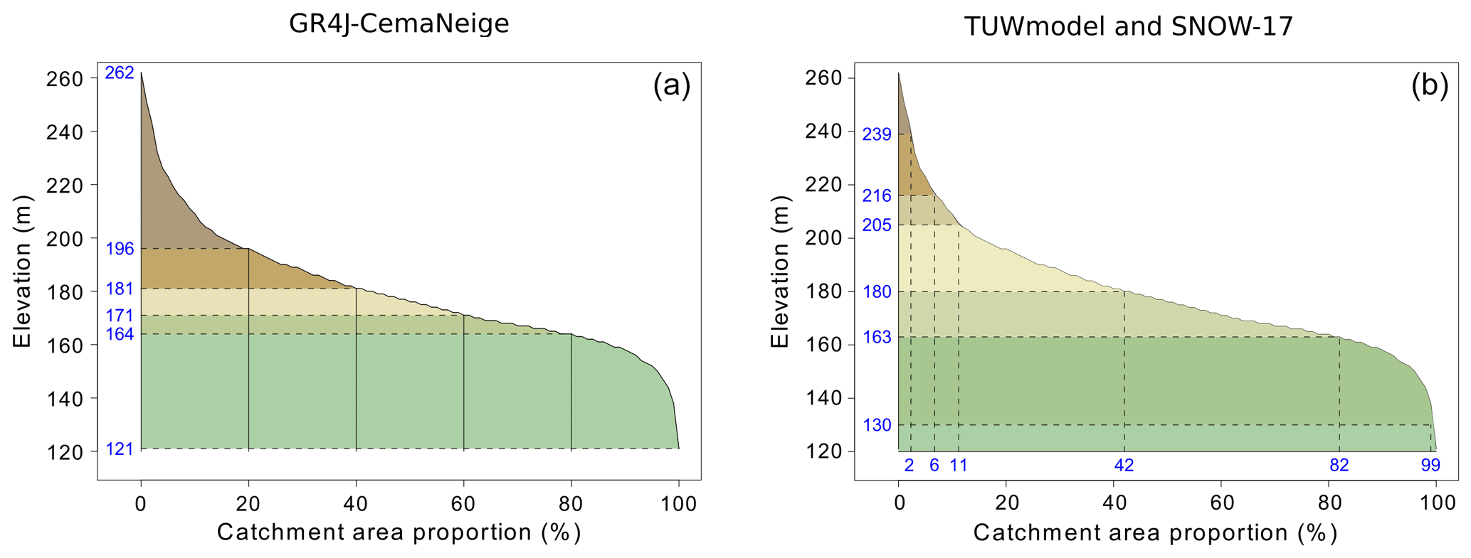
Figure 2 Example of GR4J-CemaNeige elevation zones (a) and TUWmodel/SNOW-17 elevation zones (b), with both following the hypsometric curve of the Couëtron river in Souday (France). Each colour indicates a different elevation zone.

4.2.2 From lumped models to complex semi-distributions

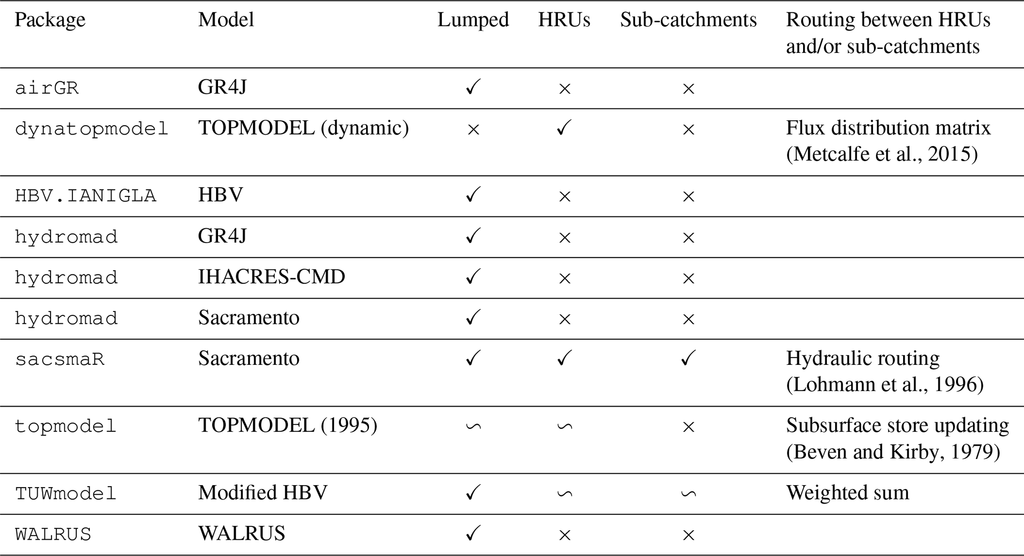
In the case of our selected models, the packages theoretically allow one or more of the spatial discretisation configurations illustrated in Fig. 3. Table 3 summarises the possible configurations for each model contained in the selected packages.

Figure 3 Illustration of the three possible spatial discretisations concerning the models contained in the selected packages for this study. From left to right are the lumped configuration, hydrological response units (HRUs) configuration and sub-catchments configuration. The catchment outline is from the Meuse river in Saint-Mihiel (France). The HRUs were generated using a function of the dynatopmodel package and are defined by the upslope area contribution based on the topographic index.

(Metcalfe et al., 2015)(Lohmann et al., 1996)(Beven and Kirby, 1979)

Table 3 Possible spatial configurations for each model. If a package allows a specific configuration (✓), then it means that the model is coded for this configuration in the related package, but it does not mean that the necessary preprocessing functions are provided. The tilde (∽) is for models following a spatial discretisation close to one of the categories.

When the models are applied with a lumped spatial configuration, inputs of precipitation and potential evapotranspiration are aggregated on the whole catchment. There is one set of parameters, which means that the model reservoirs represent the water content at the catchment scale. The model simulates a discharge output at the catchment outlet where the hydrometric record station is located.

TOPMODEL 1995 does not rely on the same calculations as dynamic TOPMODEL, especially regarding the computational units. In this implementation of TOPMODEL 1995, inputs of precipitation and potential evapotranspiration are aggregated over the entire catchment (as a lumped model) although, in the original paper (Beven and Kirby, 1979), different inputs and TWI distributions were applied in different sub-catchments. A single parameter set is defined at the catchment scale. Routines are provided for processing a digital elevation model to calculate a topographic wetness index for each grid cell (as a distributed model). The digital elevation model should have a resolution of less than 30 m for the results to be meaningful (Beven, 2012). Cells with similar values of the topographic index are then bundled to create computational units. Each unit has specific reservoirs, while the saturation zone is represented as a global saturation value at the catchment scale. These units are interconnected through the subsurface store updating based on the TOPMODEL theory and produce runoff and baseflow values to generate the final discharge time series (see Fig. 1). They can be seen as being a particular case of hydrological response units (HRUs or hydrological similarity units, HSUs, in Beven and Freer, 2001) resulting from explicit assumptions about the process response. Dynamic TOPMODEL enables the application of other types of HSUs that can be dependent on very different conditions, such as soil properties and land use but also the components of the topographic index. Fluxes between HSUs are controlled by a flux distribution matrix based on the connectivity between the grid squares of the base digital elevation map contributing to the HSUs (for more details, see Metcalfe et al., 2015, 2018). This also allows for connectivity between grids within the same HSU. Inputs can be spatially distributed, if needed, by associating each HSU with different rainfall and evapotranspiration data. HSUs, thus, have their own reservoirs. When it is required, a different parameter set can be assigned to every HSU.

The HBV model of TUWmodel enables a very straightforward spatial configuration where the model is run independently on different zones (with different parameters and inputs) which can be subbasins, elevation zones or any area defined by the user. For example, a catchment can be divided into three subbasins, with one subbasin divided into five elevation zones. The relative contribution of each spatial entity to the entire catchment is defined by the user with a weighting coefficient. The discharge outputs from each zone are then summed up using these coefficients. The Sacramento model of sacsmaR can be applied in different ways. During a preprocessing step (not provided by the package functions), the catchment can be divided into sub-catchments that can also include hydrological response units. The sacsmaR package then enables the assignment of a different set of parameters to each HRU and different data inputs. The water is run upstream to downstream through a hydraulic routing function based on Lohmann et al. (1996).

A large proportion of the packages that we have selected contain models that can be run as lumped models, though some of them can rely on a more complex spatial distribution with very specific characteristics. The most complex level of the spatial distribution is enabled by the sacsmaR package (HRUs + subbasins). Theoretically, it would be possible to run every lumped model on subbasins independently and sum the outputs with weights, as permitted by one of the TUWmodel functions. We have noticed that there are thin boundaries between the different spatial configurations. One would hardly acknowledge the differences between a computational unit of TOPMODEL 1995 and HSUs of dynamic TOPMODEL defined by the upslope area calculations. Nevertheless, these specificities can have a great influence on the final result and, consequently, the interpretations deriving from it. Please note that the high level of spatial discretisation enabled by some of the packages sometimes requires a demanding preprocessing to be carried out outside of the corresponding package (e.g. sacsmaR; see Sect. 5 and Table 6). In addition, please note that the recently released version of airGR (v. 1.6.10.4) allows for semi-distributed modelling at the sub-catchment scale using a simple lag. As this version of airGR was released after the realisation of the present analysis, it is not included in Table 3.

4.3 Model requirements and outputs

4.3.1 Inputs and number of adjustable parameters

Table 4 highlights the minimum requirements that have to be supplied to run one of the models. Other inputs can be used to increase model accuracy, such as satellite snow data to constrain the calibration of the snow function in airGR, snow cover areas for enhanced snow inclusion in HBV.IANIGLA or data concerning groundwater and surface water supply or withdrawals when running WALRUS. A digital river network can be used to set up the dynamic TOPMODEL in digital terrain analysis.

The HBV.IANIGLA package includes five configurations of the HBV routing routine. These functions rely on either three or five parameters to be estimated. The number of adjustable parameters associated with IHACRES-CMD depends on the selected routing function. When applying the exponential components transfer function with the structure identified in Jakeman et al. (1990), six parameters need to be estimated. For some models, several parameters may not require parameter estimation procedures but rather physical determination, depending on the user's need and access to additional data. For instance, in the WALRUS package, a minimum of three parameters requires the use of estimation procedures, three parameters can either be calibrated or physically determined and the other ones are derived from the physical properties of the catchment. The snow function of WALRUS has fixed parameters.

The two versions of TOPMODEL require an analysis of digital terrain data and, hence, more preprocessing work. TUWmodel and Sacramento have the highest number of parameters to adjust; however, five parameters out of 15 for TUWmodel and 10 out of 23 for sacsmaR control the snow routine.

4.3.2 Time steps and numerical resolution of model equations

The differences in terms of the time step and the resolution of model equations are summarised in Table 4. All the packages give the possibility to use their models at a daily time step. Some of them allow total flexibility (dynatopmodel, HBV.IANIGLA, topmodel, and WALRUS), which might result in errors if not correctly handled by the user. WALRUS runs with adaptive computational time steps that may differ from the input/output time steps. It is recommended that dynatopmodel and topmodel are used only at a subdaily time step (Beven, 1997; Metcalfe et al., 2015). airGR, hydromad and TUWmodel also allow time step flexibility but with some constraints. dynatopmodel implements an explicit resolution of the root and unsaturated zones equations but an implicit resolution of the kinematic wave equation between HSUs. In TUWmodel, part of the equations are solved analytically (e.g. the outflows of the upper and lower reservoirs; see Fig. 1). The other equations are solved explicitly (e.g. root zone storage). All the packages rely on operator splitting for the resolution of model equations.

4.3.3 Outputs

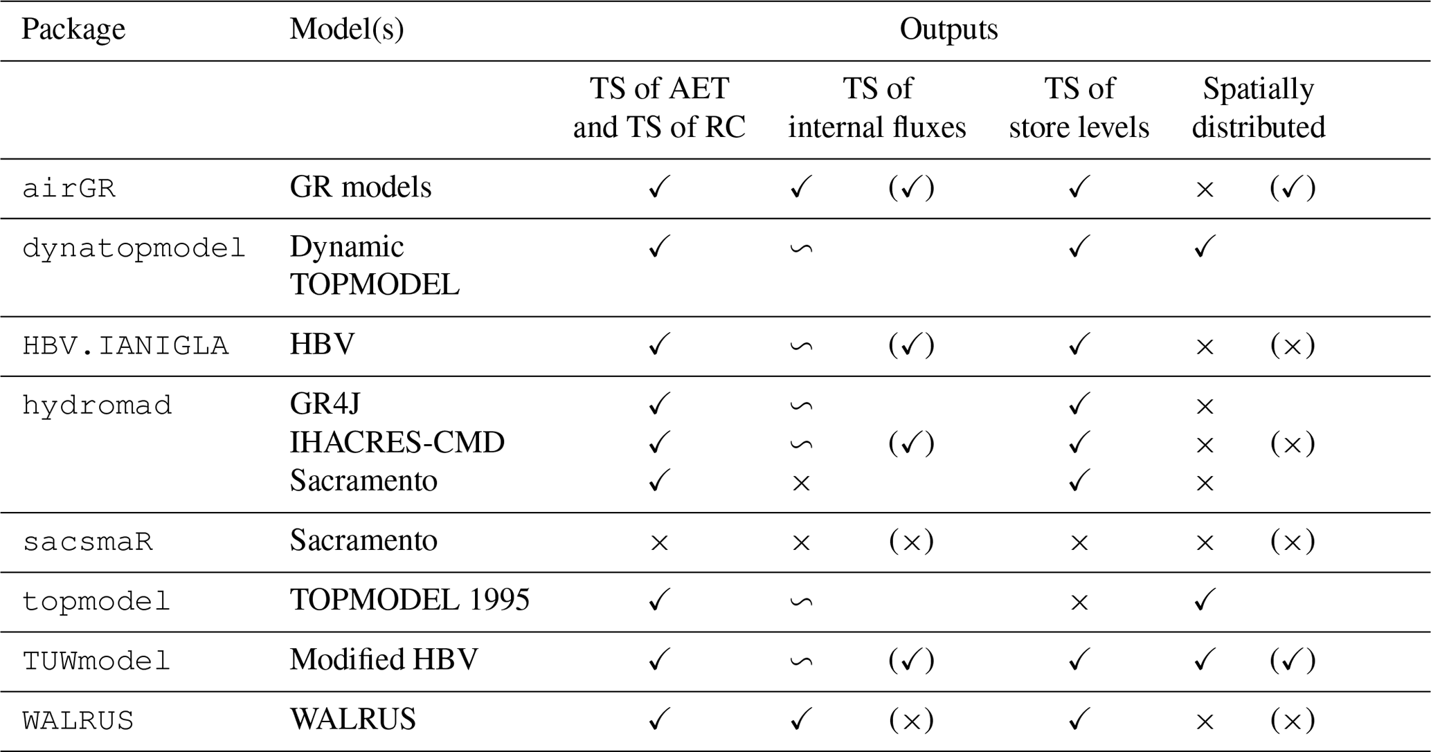
Table 5 summarises the retrievable outputs managed by the packages. While few packages allow the retrieval of all internal fluxes, most allow the user to retrieve time series of actual evapotranspiration and runoff components. Packages implementing semi-distributed models, except sacsmaR, enable the retrieval of outputs at the spatial unit scale (e.g. topographic grid for TOPMODEL 1995).

Table 4 Requirements to run the models and associated numerical resolutions. Note: D – daily; H – hourly; M – monthly; A – annual; FL – flexible; Num. res. – numerical resolution; OS – operator splitting; Ana – analytic; Exp – explicit; Imp – implicit; P – precipitation; T – air temperature; PET – potential evapotranspiration; DEM – digital elevation model; SA – subbasins area; hypso – hypsometric curve; TS – time series. The information in parentheses shows the parameters or inputs of the corresponding snow routine. It is not compulsory to provide the snow routines with the hypsometric curve, but it is strongly recommended when this is enabled by one of the packages. In this table, for the semi-distributed models, the parameters are considered uniform over the spatial units; in case they are considered distributed, the amount of parameters should be multiplied by the number of spatial units (i.e. HRUs, subbasins, etc.).

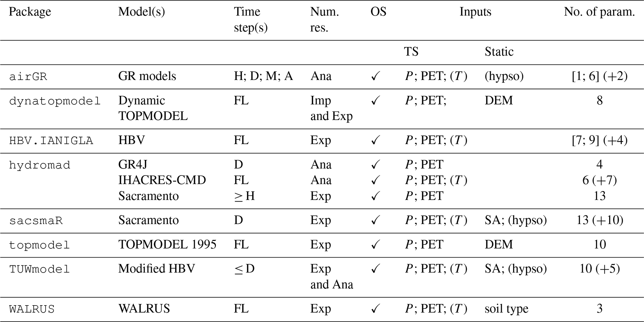
Table 5 Model outputs made available by the packages. Note: TS – time series; AET – actual evapotranspiration; RC – runoff components. The tilde (∽) indicates that only some of the time series of runoff components, internal fluxes or store levels are provided. The information in parentheses shows the outputs of the corresponding snow routine. All the packages return a time series of discharge.

The variety of models presented in this comparison are based on similar but specific assumptions in terms of storages, fluxes and spatial discretisation. The models are formulated based on our knowledge of these properties and their spatial implications. For instance, predictions of TOPMODEL and dynamic TOPMODEL can be mapped back into space because of the direct routing on the hillslopes – either implicit for TOPMODEL or explicit for dynamic TOPMODEL. It is a significant difference in terms of representing the processes in relation to catchment characteristics with other models relying on independent HRUs. These assumptions are not valid for every catchment. Consistency with a perceptual model of catchment processes should be assessed before applying one of the models contained in the R packages. Whether it is through a complex representation of shallow groundwater contribution to runoff (leading to a higher number of parameters to estimate), more conceptual calculations of soil moisture or the discretisation of a catchment into different response areas (hence, more preprocessing operations), any user will now have more materials related to what the models really imply and how these specificities are made available as outputs by the packages.

5 A critical analysis of package practicalities

5.1 An uneven set of functionalities and documentation

5.1.1 Package functionalities

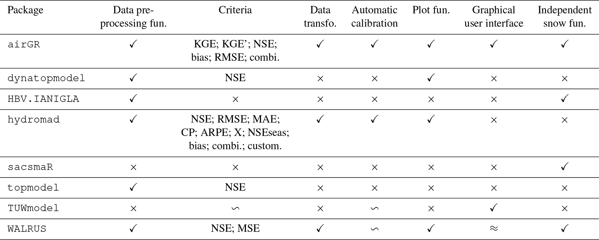
Table 6 presents whether the different packages integrate several basic functionalities to apply their models. We provide further explanations in the following.

Table 6 Functionalities provided by the packages. Note: ✓ – the item is offered by the package; × – not included; ≈ – under development; ∽ – suggested in detailed examples or presented in one of the related articles; RMSE – root mean square error; MSE – mean square error; NSE – Nash–Sutcliffe efficiency criterion (Nash and Sutcliffe, 1970); KGE – Kling–Gupta efficiency criterion (Gupta et al., 2009); KGE' – a modified version of the KGE (Kling et al., 2012); MAE – mean absolute error criterion; CP – coefficient of persistence criterion (Kitanidis and Bras, 1980); ARPE – average relative parameter error criterion (Jakeman et al., 1990); X – correlation of modelled flow with model residuals (Littlewood, 2002); NSEseas – NSE with mean of each month as the reference model instead of the overall mean; combi. – the criterion is a weighted combination of several criteria; custom. – any available criterion can be customised by the user. This table does not aim to provide guidelines for model evaluation. Other R packages can be used to assess model performance (see the explanations below).

Criteria

Weighted combinations of criteria are possible with the airGR and hydromad packages. These combinations can be derived from the implemented criteria. A combination of several criteria can be, for instance, a weighted sum of three criteria. For example, in airGR, users can average the KGE calculated on discharge, the KGE calculated on the square root of the discharge and the KGE calculated on the inverse of discharge, and different weights can be chosen for each of these three individual criteria. hydromad also offers the possibility to implement other combinations through a customisable function. airGR and hydromad include many different transformations of discharge time series. hydromad enables the calculation of the NSE on the following transformations: square root, logarithm, Box–Cox (Box et al., 2015), successive differences, monthly aggregation, triangular kernel (Silverman, 1986) and time-delay correction (Andrews and Guillaume, 2018). The user can apply other criteria on transformed data when using the customisable criterion. airGR enables the calculation of the criteria listed in Table 6 on the following transformations: square root, logarithmic (not advised for KGE and KGE'; for more details see Santos et al., 2018a), inverse, sorting from lowest to highest, Box–Cox and power. One of the WALRUS postprocessing functions returns the NSE of the logarithm of the discharges. Various R packages, such as hydroGOF (Zambrano-Bigiarini, 2020), implement model evaluation techniques that are not provided by the selected hydrological modelling packages. Fuzzy measures implemented in the fuzzyR package (Chen et al., 2019) can be used to evaluate the outputs of topmodel and dynatopmodel (for an example of application of fuzzy measures with dynamic TOPMODEL, see Freer et al., 2004). This is one way of allowing for the concept of equifinality of model parameter sets in calibration rather than trying to identify an optimum parameter set (see, for example, Beven, 2006).

Parameter estimation

Automatic calibration in the packages either corresponds to functions permitting the use of calibration algorithms from other packages with the package-specific R objects, or to the package's own algorithm. Complete examples of automatic calibration with TUWmodel and WALRUS can be found in the package documentation but do not correspond to one of the functions of these packages. The automatic calibration algorithm included in airGR derives from Michel (1991). Calibration algorithms implemented in other R packages can be used within airGR, as documented in a vignette. In the hydromad package, nine automatic calibration algorithms are proposed, either using built-in R functions (optim()), implementations within the package (shuffled complex evolution), or external packages, e.g. the differential evolution algorithm (Storn and Price, 1997) enabled through the use of the DEoptim package (Ardia et al., 2020). Parameter estimation and uncertainty quantification are important steps of the hydrological workflow. Multiple sources of epistemic uncertainty are associated with simulations of hydrological models (Beven, 2016), such as uncertainty in the available catchment data that can lead to incorrect model inference (Beven, 2019) or uncertainty arising from the difficulty models have in representing the properties affecting river flows. Several methods can be used to take uncertainty into account when estimating model parameters. For example, hydromad includes a function to determine feasible parameter sets and estimate prediction quantiles by applying the generalised likelihood uncertainty estimation (GLUE) method. The FME package (Soetaert and Petzoldt, 2010) enables the estimation of parameters within a Bayesian Markov chain Monte Carlo (MCMC) framework.

Plot functions

The plot function of airGR can display several variables (e.g. Fig. A1), including time series of precipitation, potential evapotranspiration, actual evapotranspiration, temperature, snow water equivalent, simulated discharge, observed discharge and simulated minus observed discharge (residuals), interannual monthly median, the correlation between observed and simulated discharge, and cumulative frequency. dynatopmodel contains a function to plot the observed and simulated hydrographs along with the precipitation and actual evapotranspiration time series (mainly designed for short time series, e.g. Fig. A2). hydromad integrates a function to plot simulated and observed hydrographs (including different simulation configurations and rainfall time series; e.g. Figs. A3 and A4). This function can also plot the flow error, i.e. the criterion value for each point of the time series. A function to select and plot discrete events is also included in hydromad. WALRUS includes two functions to display the model outputs. The first one enables one to plot the time series of observed discharge, simulated discharge, precipitation, potential evapotranspiration, modelled groundwater drainage, modelled actual evapotranspiration, wetness index, soil reservoir and surface reservoir levels, seepage and surface water supply or extraction (e.g. Fig. A5). The second function displays the model residuals, the autocorrelation of residuals and the cross-correlation between residuals and the precipitation time series.

Graphical user interfaces

airGR and TUWmodel offer a graphical interface for manipulating the models. A WALRUS graphical user interface (GUI) is currently under development (see Sect. 4.6 of Brauer et al., 2017). The airGR and TUWmodel GUIs rely on the shiny package (Chang et al., 2019) that implements an R framework to build a web application. The GUI developed for the airGR package is proposed in the airGRteaching package (Delaigue et al., 2018, 2020a). This GUI is either available online (https://sunshine.irstea.fr/, last access: 20 September 2020) or by launching the interface from R. This GUI integrates several features (see Fig. B1), e.g. by easily estimating the parameters either manually or automatically. To perform an automatic calibration, users have to select an objective function among the NSE and KGE, calculated on flow time series (TS), flow inverse TS or the square root of flow TS. They can then directly visualise the impacts on seven criteria values (including those mentioned previously and the flow bias) and through several graphics. For both types of calibration, it is possible to adjust the temporal window on which the model performs (using a slider or by selecting the period on the graphic). The following four graphical panels are available: precipitation TS, simulated and observed hydrographs and flow error TS (e.g. Fig. B2a); a concise performance graphic displaying the TS of precipitation, simulated and observed hydrographs, interannual monthly median, the correlation between observed and simulated discharge and cumulative frequency (e.g. Fig. B2b); TS of store levels and runoff components (e.g. Fig. B2c); a model diagram displaying store levels, fluxes and unit hydrographs at each time of a selected temporal window (e.g. Fig. B2d); and a fact sheet with several hydrometeorological characteristics of the selected catchment (e.g. Fig. B2e and B2f). The simulation results and plots can be downloaded by users.

The TUWmodel GUI (Sleziak, 2019) is available online (https://webaapptuwmodel.shinyapps.io/TUWteaching/, last access: 20 September 2020). This interface includes five example data sets on which the TUWmodel parameters can be manually adjusted (see Fig. B3). Users can adjust the parameters and directly observe the impacts on a graphical panel that displays the simulated hydrograph compared to the observed hydrograph and the TS of three state variables (e.g. Fig. B4a). This interface also offers a second panel that allows users to visualise the localisation of the five catchment outlets on a map along with their area, mean elevation, mean slope, forest cover percentage, mean annual precipitation, mean annual air temperature and mean annual runoff (e.g. Fig. B4b).

5.1.2 Package documentation and support

Table 7 presents whether the main functionalities of the packages are provided with sufficient explanatory documents. Table 8 summarises the available additional documentation that can help to better understand the characteristics of the models and the packages.

Table 7 Assessment of package documentation. Note: Description – information on the general purpose of the function and the associated possibilities; details – precise explanations of the function; arguments – description of the function arguments that requires details about the unit, the R object class and how to obtain it; value – description of the function outputs; references – related documentation where users can find more information on the function; examples – R commands to use the function (examples are considered as being comprehensive if they cover most of the functionalities and if there is an example for each function); data set – an example data set is provided and can be used with the package functions; steps between functions – explanations of the required stages to run the main functions. The last two fields are not explicit parts of the package manuals but can help one to understand and use a package.

The topmodel's main example does not provide information on the preprocessing steps to discretise a catchment. It may be complicated to use sacsmaR to run the semi-distributed version of Sacramento because the example found in one of the vignettes does not illustrate the required discretisation. Coherence between dynatopmodel functions is not made explicit by the provided function, especially for the catchment spatial discretisation. All the packages, except HBV.IANIGLA, include data sets that can be used with the examples provided in the documentation. HBV.IANIGLA provides an example on how to generate random time series of inputs.

Coron et al. (2017)Metcalfe et al. (2015)Andrews et al. (2011)

Table 8 Additional available package documentation and support. Note: @ – email; GL – GitLab; GH – GitHub (URLs in this table were last accessed on 20 September 2020).

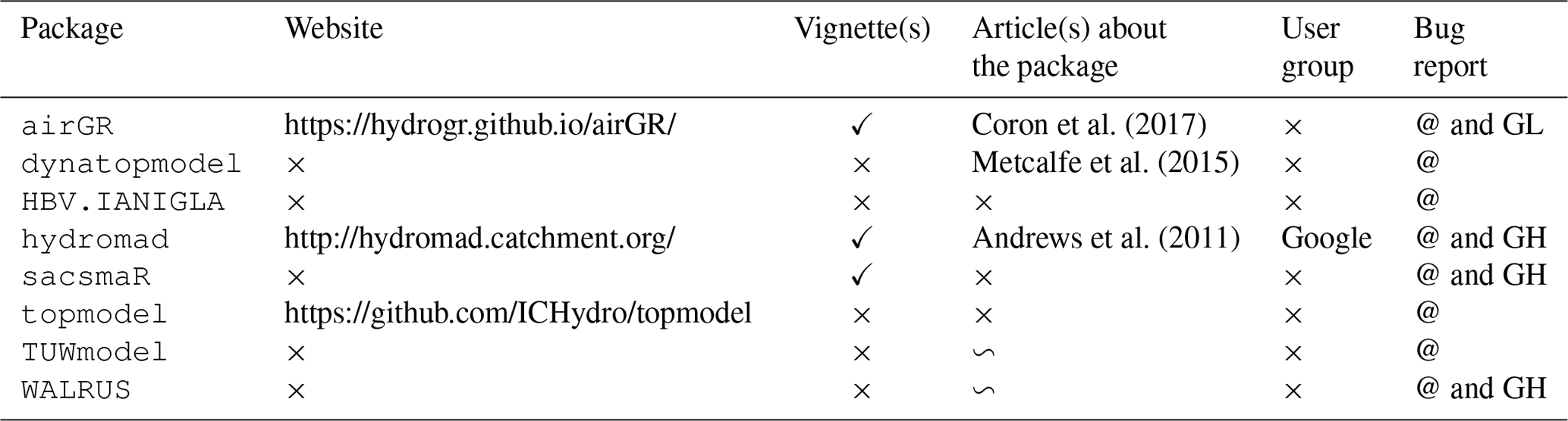
airGR includes several vignettes, for example on how to estimate parameters within a Bayesian MCMC framework. The WALRUS package is stored on the GitHub platform, where a complete set of documents, tutorials and data can be found (e.g. an R script to run a Monte Carlo parameter estimation procedure). A comprehensive user manual, with a structure that is different from the usual R documentation, can also be found on GitHub. sacsmaR is stored on GitHub with a vignette on how to use the different functions. hydromad offers a vignette, and nine demonstrations are available that deal with subjects such as how to estimate the model parameters or how to conduct a sensitivity analysis. Examples of sensitivity analysis and GLUE method (Beven and Binley, 1992) are available on topmodel's website. Articles related to the TUWmodel and the WALRUS packages were not written to present the packages themselves but rather the models included in these packages. Other examples of TUWmodel were found in the appendixes of Ceola et al. (2015). Users are invited to report bugs or ask for additional support via email and, for some packages, by creating GitHub (hydromad, sacsmaR and WALRUS) or GitLab (airGR) issues. A user group related to the hydromad package is available for additional support.

Looking at Table 6, it appears that there is an important heterogeneity in the availability of package functionalities. Packages such as airGR, hydromad and WALRUS integrate many functionalities from data management to analyses of the results, whereas the other packages mostly contain the main functions to run the associated model. We can differentiate the following two types of packages in our study: packages guiding the user with functionalities in line with the hydrological workflow and, to a certain extent, constraining the use to reduce potential errors and packages allowing more flexibility but less guidance and, thus, potentially more errors. Regarding the documentation, packages with the most functionalities also provide more comprehensive documentation and additional documents. Even if dynatopmodel and TUWmodel offer more explanatory documents and examples than sacsmaR and topmodel, there is still a lack of information concerning the spatial distribution that these four packages permit (see Sect. 4.2). This is an important issue because it is crucial for users to be able to use all the functionalities of a package. The more complex the models are, the more important the functionalities and, therefore, the provided explanatory documentation become; hence, strengthening the documentation associated with some of the presented packages is necessary to assure more rigorous applications of the models.

5.2 A guide for user implementation

Considering the previous analysis along with package distinctiveness in terms of R implementation raises the question of how to use the packages containing hydrological models. Figure 4 shows the links between the main functions required to apply each package on a simple hydrology example (R scripts are provided in the supplementary documentation; Astagneau et al., 2020).

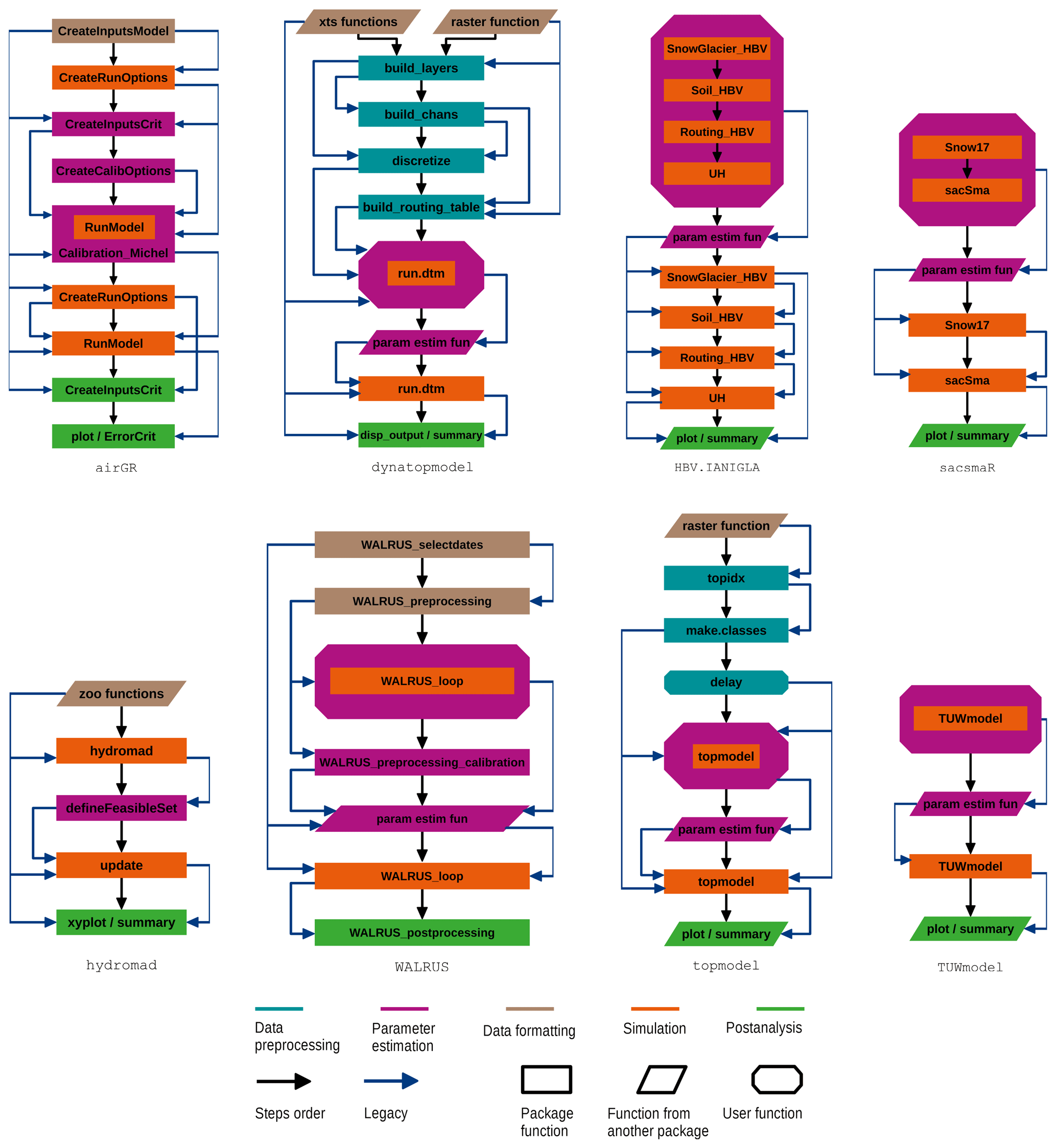
Figure 4 Unified diagrams illustrating the package main functions that are necessary to proceed with parameter estimation and validation on a basic example in hydrology modelling. R core functions are not explicitly illustrated. Basic data preprocessing steps, such as checking data gaps and consistency, are not displayed on this diagram, but it is strongly recommended to adopt such practices before operating a model. Users can run hydromad.options and hydromad.stats to change or visualise the options for parameter estimation in hydromad. Many different parameter estimation methods are available within the R environment or within the selected packages. Note: legacy – a function depends on other functions to be operable (e.g. its arguments are obtained by running another function); user function – users have to write their own R function integrating, among others, the legacies illustrated on the diagrams.

The diagrams of Fig. 4 indicate three main groups of packages in terms of R implementation:

1. airGR, hydromad and WALRUS integrate many R functions with complex connections and inner consistency. These choices regarding the R implementation follow similar steps from data formatting to result analysis. They aim at reducing potential errors arising from R codes written by the modeller, whose choices are guided throughout the hydrological workflow. They also ease the application of a new model by end-users.

2. sacsmaR, TUWmodel and HBV.IANIGLA, on the other hand, whose functionalities are less extensive, rely on a very simple R structure. R objects preparations are left to the user (i.e. without particular specifications or requirements), who has to provide vectors of data time series. The sacsmaR and TUWmodel packages do not contain preprocessing functions to use their models with the spatialisation specificities explained in Sect. 4.2. As the packages only integrate functions allowing one to run the core models, the R structure only depends on the models inputs and outputs, whether it is with one function integrating all the modules of the model (TUWmodel) or with separate components (HBV.IANIGLA and sacsmaR). Unlike what is offered by the packages of the first group and dynatopmodel, the user has to code the desired plots by using the runoff outputs.

3. As pointed out in Sect. 4.2, operating the two versions of TOPMODEL requires spatial discretisation preprocessing steps. dynatopmodel and topmodel integrate these steps at the beginning of the workflow through more (dynatopmodel) or less (topmodel) complex functions and connections. The spatial operations also require the use of an external package to deal with raster data. The remaining steps in the workflow are then very similar to those of the second group of packages.

airGR and hydromad contain parameter estimation functions and objective functions that are integral parts of their structure, whereas users have to build their own objective function and combine it with an external algorithm when operating the other packages. WALRUS includes the structural functions to facilitate parameter estimation. TUWmodel and WALRUS provide examples of how to proceed with these steps.

The path to better guidance and avoiding mistakes in the application of the models – which implies more rigorous methods that include, for instance, uncertainty analyses – is a tricky road facing the wide heterogeneity of packages in terms of R structure and models in terms of modelling choices. One could imagine better harmonisation of packages taking advantage of other packages' strengths (e.g. using a similar structure for the objective function or managing time complexities with the same R functions). This goal is not out of reach and would considerably improve the usability and scope of these packages. It would require defining sampling strategies for parameter estimation (e.g. with the differential evolution adaptive metropolis (DREAM) algorithm; Vrugt and Beven, 2018) and post-processing techniques for performance and uncertainty assessments. Some hydrological modelling R packages include these strategies, and some leave them as external packages (see Sect. 5.1.1). This first attempt at categorising the packages in terms of R implementation along with the provided R scripts should ease the application of packages containing hydrological models.

5.3 Analysis of R structures and CPU times

5.3.1 Programming languages and dependencies

Some packages are entirely coded in R, which is an interpreted language, and some integrate models coded with a compiled programming language interfaced with R, e.g. Fortran (Backus et al., 1957), C (Kernighan and Ritchie, 1978) or C$++$ (Stroustrup, 1984, see Table 9). When the model functions are coded in a compiled language interfaced with R, users may not have direct access to all the code required. Computation times tend to be lower when using a compiled programming language rather than using an interpreted one (see Sect. 5.3.2). As the most part of the necessary CPU time is dedicated to the actual hydrological model run, some package developers chose compiled languages for the model calculations. There are three packages that integrate models entirely coded with the R language and four packages with a compiled programming language (C, C$++$ or Fortran). The hydromad package integrates some models coded in R, some in C or C$++$ and some with both implementations to facilitate both debugging and fast execution.

Table 9 Programming languages of the models used in the selected R packages.

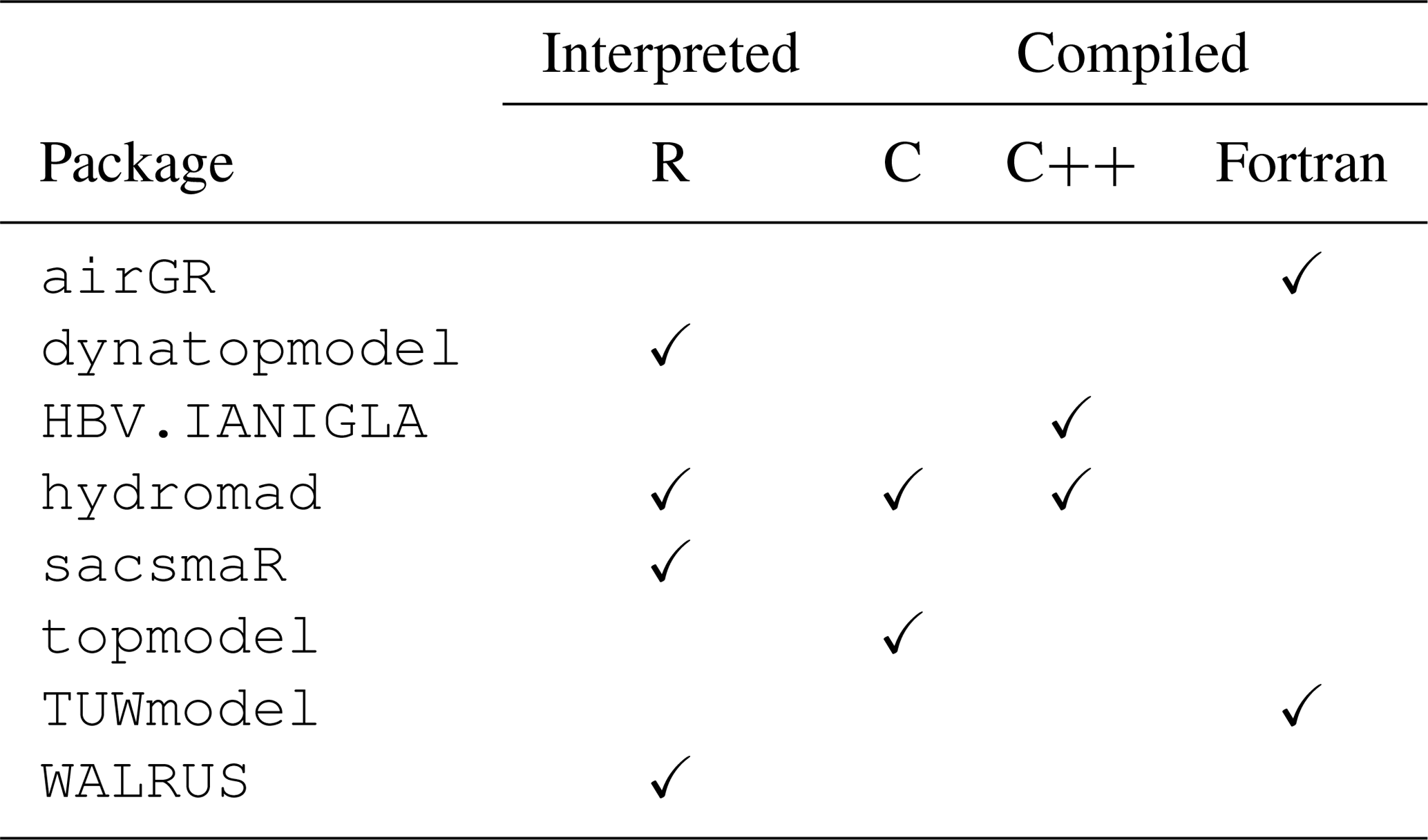
Table 10 summarises whether packages require other packages to run the models. In total, three of the selected packages integrate functions requiring the use of external packages. dynatopmodel has the highest number of dependencies (nine packages), hydromad has six dependencies and WALRUS has one dependency. These three packages rely on several types of external packages. Some of these external packages (e.g. zoo, Zeileis and Grothendieck, 2005) integrate functions to manage time series. dynatopmodel relies on packages integrating functions to deal with spatial data (e.g. raster, Hijmans, 2020). Some packages are employed to solve equations or proceed with specific calculations (e.g. calculations on univariate polynomials with polynom; Venables et al., 2019).

Table 10 Package dependencies. Base packages and recommended packages are not explicitly taken into account in this table.

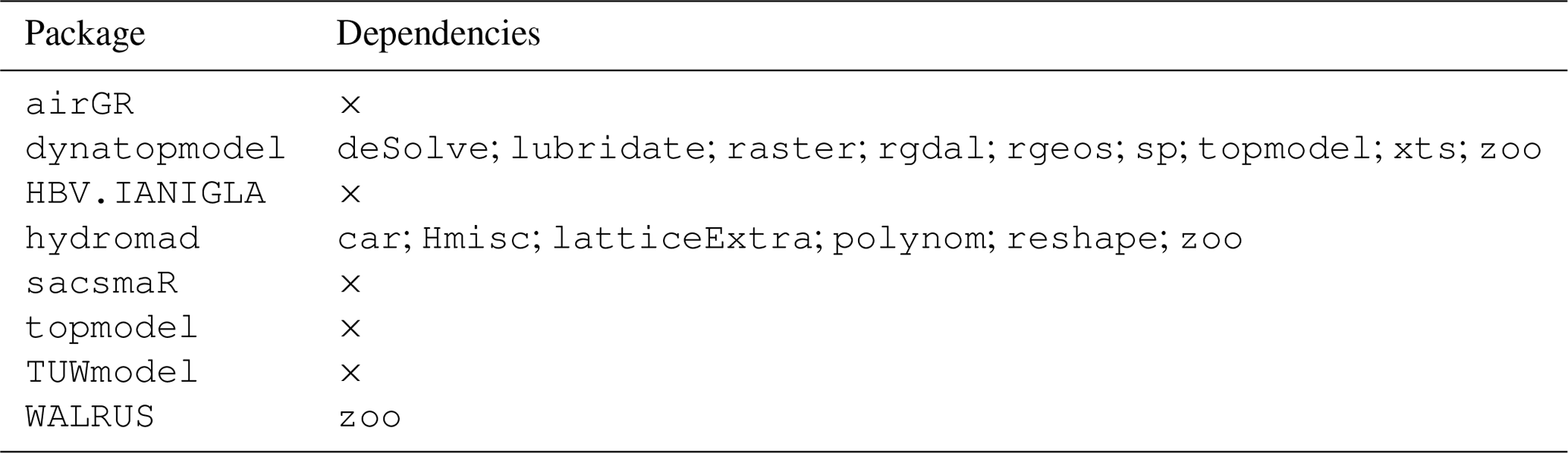
5.3.2 CPU times

We hereby present the CPU time required for one model run with the selected packages (Fig. 5). As the hydromad package includes two implementations of the GR4J and IHACRES-CMD models, one coded in R and one coded in C (see Sect. 5.3.1), computation times were estimated for both implementations. Note that WALRUS computation times can vary depending on the selected parameter set.

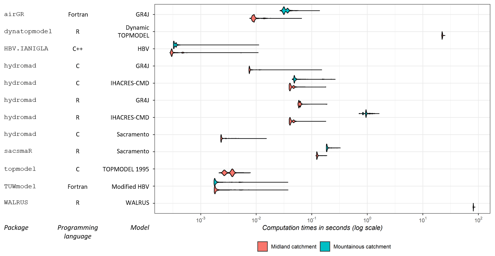
Figure 5 Computation times of the packages (time of one run estimated from 1000 runs using the same parameter set with the microbenchmark package). The models were run on a French catchment, the Meuse river in Saint-Mihiel, and a mountainous catchment, the Ubaye river at Lauzet-Ubaye, for a 10-year period at a daily time step. The related package functions were applied using the default settings, i.e. on a single spatial unit, except for dynatopmodel and topmodel. Runs on the mountainous catchment were performed only with the packages that integrate a snow function and use the default settings (i.e. five elevation bands for airGR and one for the other packages). hydromad includes an R version and a C version of GR4J and IHACRES-CMD. Data preprocessing and formatting are not taken into account in the estimation of computation times. Computer characteristics are as follows: RAM capacity – 8.00 GB; CPU – Intel i5-8250U 1.80 GHz; OS – Windows 10 (64 bit). R version 3.6.0 (64 bit) was used.

The results of Fig. 5 show that the packages based on models coded with a compiled programming language have lower CPU times than the packages integrating models coded in R. The CPU times associated with the packages integrating models coded with a compiled language have the same order of magnitude. The HBV.IANIGLA package has lower CPU times than the other selected packages. The CPU times associated with sacsmaR and the models coded in R of hydromad are lower than the CPU times of dynatopmodel and WALRUS (CPU times can also depend on the model implementation). WALRUS has the highest CPU times, which is probably caused by the flexible time step approach, where the computational time step is decreased automatically to improve numerical stability. For all these packages, the runs performed with the associated snow function resulted in higher CPU times than for the runs without the snow function, except for TUWmodel, which does not integrate an independent snow function. Note that computation times may differ when selecting other function settings and model configurations.

6 Discussion

Following these analyses of hydrology modelling R packages, we discuss how users can actually apply one of the models offered by the selected packages to a specific application or research question, we identify what improvements could be brought to the packages, and we discuss the reasons and the implications of the implementation choices that were made on the packages.

6.1 Usefulness of the proposed analysis for end-users

While our analysis focuses on models that can be considered as conceptual rainfall–runoff models, we have highlighted different approaches, assumptions and choices underlying these models, both in terms of structure and spatial discretisation, which imply distinct numbers of parameters and sometimes specific inputs.

6.1.1 Choosing the fit-for-purpose model and package

This attempt to simplify the users' selection process does not aim at labelling good and bad models or packages and, therefore, cannot shed light on which models hydrologists should use today. In our opinion, two major points should be drawn from this study in terms of hydrological modelling. First, this work should be considered as a tool to determine which models, within the R environment, best fit the specific requirements of the end-user and their perceptions about the dominant processes in a catchment (see the stages in the modelling process in Beven, 2012). For instance, we do not advise running the WALRUS model on steep mountainous catchments; however, the model is suitable for lowland catchments with shallow groundwater. WALRUS was also designed for catchments where ditches and channels have great influence on river flows and can take into account major water withdrawals or surface water supply. Interestingly, only WALRUS integrates modelling aspects related to catchments affected by human activities, and none of the selected packages offers functions to take the regulation of dams into account. Simulations on catchments with a high proportion of solid precipitation should be performed with models integrating functions to take snow into account (e.g. the HBV models of HBV.IANIGLA and TUWmodel, the Sacramento model of sacsmaR and the CemaNeige model of airGR). The dynamic TOPMODEL can be relevant for simulating river flows in catchments with high spatial heterogeneity of precipitation (e.g. with frequent storms) since it integrates a finer spatial discretisation. This discretisation requires at least a digital elevation model. These examples certainly do not cover the numerous applications enabled by these models but can help users to reason when selecting a hydrological model implemented in the R environment. Second, our analyses address what is enabled by the packages when considering these modelling specificities. For instance, users can theoretically run the complex semi-distributed version of sacsmaR but would need to prepare the spatial discretisation with external R packages or software. While HBV.IANIGLA implements the HBV model with separated functions, TUWmodel includes one function for the whole model – although calculations on separate zones are implemented, which can improve snow calculations. dynatopmodel enables a different set of parameters and inputs for each computational unit (eight parameters), whereas topmodel integrates a version based on 10 adjustable parameters (including two initialisation parameters), but the model can be run with a less complex spatial version requiring fewer preprocessing procedures.

6.1.2 Towards helping users to use new models appropriately

Appropriately using a new model is fundamentally difficult. Understanding the complexity resulting from the different modelling choices, the model inner consistency and whether it is appropriate for a specific research problem also depends on the perceptual model of the hydrology of a catchment (e.g. Wrede et al., 2015; Beven and Chappell, 2021). Adding the difficulty of implementation in terms of software or programming language complicates this task even more. Flexible modelling frameworks, such as SuperflexPy (Dal Molin et al., 2020) and FUSE (Clark et al., 2008), have partially addressed these difficulties. However, their complex conceptualisation makes them more accessible to advanced modellers than to newcomers. The FUSE implementation for R available on GitHub is in need of active maintenance by the community (https://github.com/cvitolo/fuse, last access: 20 September 2020). The hydromad R package provides such a flexible framework to a certain point, as it enables one to combine different soil moisture accounting functions with several routing modules. It is one of the reasons that should encourage users to model within the same framework. Such a framework can be the R environment with the available modelling packages. But for these packages to be powerful tools and still maintain a certain degree of practicality and accessibility, they need to be strongly documented and user-friendly. In this regard, implementing modelling functionalities can guide users towards good practices and help them to interpret results. However, enough flexibility should be maintained to allow other applications not considered by authors. Package developers must find the right balance when adding functionalities, in an attempt to help users run models with more possibilities, without making the package implementation excessively complex. It means that packages are made accessible for newcomers but are still of interest to more experienced hydrologists. In this respect, GUIs are interesting features to make packages more accessible to newcomers and to users that are not familiar with coding, especially for students. They allow users to understand what the models imply in terms of fluxes, parameters and stores by providing easy tools to perform basic simulations. Given that these GUIs are less flexible than the packages themselves and do not enable all the modelling aspects, they are not intended to replace the packages. They can be considered as convenient tools to help users in their understanding of the models and, therefore, facilitate the selection process. These tools are improvements to guide users in their applications of the different models and could be considered for future developments of the selected packages, as we have seen that only two packages provide a GUI (airGR and TUWmodel). Learning the idea of calling functions is, however, important, as it provides a more transferable way of thinking.

6.2 Possible improvements for the packages

6.2.1 The fifty shades of R package functionalities

With respect to our list of packages, we have seen that three main groups of packages emerged from our analyses of practicalities. airGR, hydromad and WALRUS offer the most functionalities to run their associated models and, therefore, rely on more functions integrated in a complex structure and associated with extensive documentation. Providing functionality such as graphical outputs or performance criteria is a major advantage for users that can easily and quickly have access to an overview of model performance. This does not restrain users in their modelling assessments, as graphics and criteria can be coded within the R environment when accessing the model outputs made available by the packages (see Table 5). Do these packages allow enough flexibility for other applications and users? On the one hand, we have been able to calibrate models from three packages using the same automatic calibration algorithm, namely the DEoptim package (Ardia et al., 2020), which is an indicator of adaptability. On the other hand, there are still improvements to be made. For instance, the performance criteria included in airGR require specific airGR objects to be calculated. Users cannot directly use time series of other variables in the related functions that would, for instance, enable the comparison of simulations from two different packages. hydromad enables the estimation of adjustable parameters with different algorithms via several external R packages, but the documentation does not yet integrate examples on how to use its structure with other algorithms, i.e. new R algorithms that are not included in the structure of hydromad.

The second group of packages, offering fewer functionalities with a simpler R structure, includes HBV.IANIGLA, sacsmaR and TUWmodel, though TUWmodel provides more extensive documentation. This type of implementation, as flexible and easy to use as it seems (i.e. fewer steps, dependencies and functions on the diagrams of Fig. 4), does not always end up being easy to use or to apply to specific uses. When guidelines are not sufficiently provided, it can lead to more errors and the misuse of the models. For example, the documentation of HBV.IANIGLA does not provide information on how to manage missing values, which usually occur in flow time series. sacsmaR does not provide functions for spatial discretisation or examples on how to proceed by using functions from packages. This exposes users to misuse and errors. Even though sacsmaR is theoretically adaptable, using the Sacramento model with a finer spatial discretisation is very complicated with this package. While TUWmodel does not offer many functionalities, its documentation provides guidelines for basic uses.

dynatopmodel and topmodel (third group) include the basic spatial discretisation functions to run their version of TOPMODEL. These functions guide users for simple applications of the model. However, few guidelines are given for more complex applications that are enabled by the packages (for example, information on how to create hydrological response units with maps of land use or soil type when using dynatopmodel). As dynatopmodel integrates a more complex spatial distribution, its structure is more complex and, therefore, harder to implement. More functionalities could have improved its usability, although it is more adaptable to other applications in its present form.

6.2.2 On the importance of accounting for uncertainties

airGR and hydromad include parameter estimation functions as an integral part of their structure. TUWmodel and WALRUS provide some examples on how this can be achieved with external packages. However, the four other packages do not present guidelines regarding this step in the hydrological workflow. Parameter estimation is an important step for these hydrological models. It is also important to understand how to manually estimate parameters and to avoid unrealistic parameter values. As imperfect as some of these procedures might be, as highlighted by Beven (2012, 2016), regarding, for instance, the inclusion of epistemic uncertainty (Beven, 2019), the related documentation is lacking in some of the selected packages (note that topmodel includes an example to test different sets of parameters).

Taking different sources of uncertainty into account, especially epistemic uncertainty in data inputs (Beven, 2019), is important when working with models considered as hypotheses about how a catchment is functioning (e.g. Andréassian et al., 2009; Clark et al., 2011; Beven, 2016; Blöschl, 2017). It enables one, for a specific case study, to reject a model that would yield poor predictions due to wrong hypotheses not brought to light by highly uncertain evaluation data (Beven, 2016, 2018). This important step in the hydrological workflow is mentioned in the documentation of four of the selected packages (airGR, hydromad, topmodel and WALRUS). Uncertainty analyses could, therefore, be more strongly documented in future versions of the packages to guide users towards more rigorous applications of the models. Although the proper way of including these uncertainties is debated among hydrologists, e.g. regarding the non-stationarity of epistemic uncertainty (e.g. Koutsoyiannis and Montanari, 2015; Beven, 2016), testing of alternative model structure hypotheses (e.g. Clark et al., 2011) or the definition of the limits of acceptability for model rejection (e.g. Beven, 2016, 2018), this highly debated question is beyond the scope of this paper. Nevertheless, hydrologists who intend to apply any of the packages presented in this study should be encouraged to perform uncertainty analyses. In this regard, several methods can be used within the R environment, such as GLUE or MCMC analyses.

6.3 Aspects of practical implementation and maintenance of packages

The adaptability and efficiency of packages can also be assessed in terms of R structure. The choices that developers have made for their R packages, programming languages used for the core functions of the models and dependence on external packages for some functions have resulted in very different R structures. Using a compiled programming language for the core model functions (airGR, HBV.IANIGLA, hydromad, topmodel and TUWmodel) tends to lower CPU times and ease parameter estimation procedures, though computation times can also depend on algorithm efficiency, the choice of parameter estimation technique, number of parameters to be estimated and operations not related to the core model runs. As a result, applications on studies relying on a large database of catchments and uncertainty analysis procedures, such as Monte Carlo realisations, are easier with these packages. On the other hand, this does not facilitate the comprehensibility of the packages, as users who would want to understand the core function algorithms would need to learn another programming language. Coding all the functions in R (dynatopmodel, sacsmaR and WALRUS) improves the comprehensibility of the core functions of a model. This also allows users to change the model algorithms directly within the R environment. However, depending on the implementation, this alternative can increase computation times and, therefore, restrain users in their application of the hydrological models. Relying on external packages is a way of taking advantage of the many possibilities offered by the packages of the R environment, which can improve the functionalities of a package. However, package dependencies can become a liability when the versions of the external packages change (an issue that is not specific to the R language). This sometimes induces errors with functions that can no longer be run by users, which could, thus, reduce the durability of R scripts and, therefore, the transferability and understanding of methods and results.

Slater et al. (2019) identified key points for future developments of R in hydrology that would improve the transferability of methods. A structured approach when developing a package, user-friendly functions and the documentation are in line with the specific results of our analyses of practicalities. Developers are advised to consider these analyses, as R packages implementing hydrological models have the advantage of avoiding the requirement to recode the model or buy a specific software. Even if users need to learn the basics of the R language to employ one of these packages, this allows many modellers to save time and focus on modelling rather than algorithm issues. Furthermore, despite the need for some improvements, using a package for hydrological modelling within the R environment is greatly enhanced by the package follow-up maintained by a strong community of developers and users. Bugs and requests can be reported via e-mail for all the packages (see Table 8). Ensuring follow-up to help users understand package specificities and to deal with errors and misuse is a way for more reusable methods and more rigorous applications of the models. It also allows users to follow the latest developments through version controlling, thus ensuring R script durability (version controlling of airGR is accessible via the GitLab platform; WALRUS, hydromad and sacsmaR version controlling are accessible via GitHub; older versions of the four other packages are archived on the CRAN). This two-way interaction between users receiving help with their specific applications and developers that can improve their packages is essential to keep the R environment being a helpful framework for hydrologists. In this sense, several developers within the hydrological science community have been committed to allow the open-source use of hydrological models in the form of R packages.

7 Conclusions

Given that the R language can easily be operated for hydrological purposes, the growth of available modelling packages makes the choice of an appropriate package more complicated. To identify the barriers and opportunities for any hydrologist employing one of the packages, we have first proceeded with a careful analysis of a selection of models contained in eight packages. These models were examined in terms of conceptual storages and fluxes, spatial discretisation, requirements and retrievable outputs. We have then evaluated the packages regarding their practicality, i.e. the integrated technical features, the related documentation, the R hydrological workflow, CPU times and the programming languages interfaced with R. The results of our unified analyses confirmed that the selected models rely on different assumptions with regards to the conceptualisation of the water cycle and, therefore, their emphasis on the main physical processes contributing to river flows. A model structure can be selected, depending on our knowledge of the physical properties of a catchment. As the understanding of these properties is limited, hydrological models are subject to epistemic uncertainties (e.g. Beven, 2016), making them imperfect but improvable tools for different purposes in hydrology. The spatial discretisation options that are theoretically enabled by the packages range from lumped conceptualisation to a finer spatial discretisation integrating both HRUs and subbasins. These modelling specificities result in variations concerning the requirements of each model. Packages enable more or less flexibility with respect to these modelling characteristics in terms of time steps and retrievable outputs. While finding differences in model conceptualisations and technical features offered by the packages was expected, we did not expect such heterogeneity regarding what the packages enable. Indeed, some packages provide functions, from data preparation to result analysis, in line with the hydrological workflow, whereas some others do not provide enough features and guidance to allow the user to operate the models with external functions and with reference to other documents. Such choices by the package authors raise the question of the initial purpose behind the development of these packages. Whether it is for teaching purposes or complex hydrological studies, detailed documentation is always important to ensure reusable methods and appropriate use of the packages.

Our analysis aims to help the R users to select the packages that best suit their requirements. The provided framework containing examples on how to use the models included in the selected packages represents a first step towards more comprehensible and operable R packages for hydrological modelling. With the same aim, the unified representations of the usability of models and packages result in strengthened materials associated with these specific packages. While some limitations regarding package practicalities have arisen from our analysis, we hope that our framework will help developers in improving their packages by providing more transferable methods. We also note there are numerous features currently under development that were not examined in this article.

Despite a thorough selection of packages, some of them were discarded from the analysis. Indeed, as pointed out in Sect. 2.1, some hydrological models with more data requirements and very different purposes exist in the R environment but were not included in our study. Furthermore, one might ask whether the choice of package should exclusively rely on the performance of the models. We could argue that, in conceptual hydrology modelling, models are mainly assessed by their ability to reproduce river discharges at the gauging station of a catchment (Singh et al., 2017). Therefore, a hydrologist who would need to use an R package for modelling might favour the efficiency of a given model in their selection procedure. Even though we have run the models contained in the selected packages several times on different data sets, we have chosen to not show any comparison of model performance, which would be dependent on specific catchment characteristics and more representative of the model than of the package itself. We provide with this comparison R scripts to test one parameter set for each model on a simple hydrology example, whereas it is becoming increasingly important to be able to use sensitivity analysis to explore the location-specific behaviour of a model (Haghnegahdar et al., 2017; Blair et al., 2019), to perform uncertainty and identifiability analyses to understand the ability to estimate parameters (Guillaume et al., 2019), to test alternative model structure hypotheses (Clark et al., 2011) and to define limits of acceptability for model rejection (Beven, 2016, 2018). Comparison of models implemented in R with others in Python, MATLAB or proprietary packages is similarly left to future work.

This work could be considered as an early stage version of a meta-package that would manage to run all the packages through the same R architecture, thus improving guidance, appropriate constraint and reliable comparisons when using hydrological models with R.

Appendix A: Plots by some of the selected packages

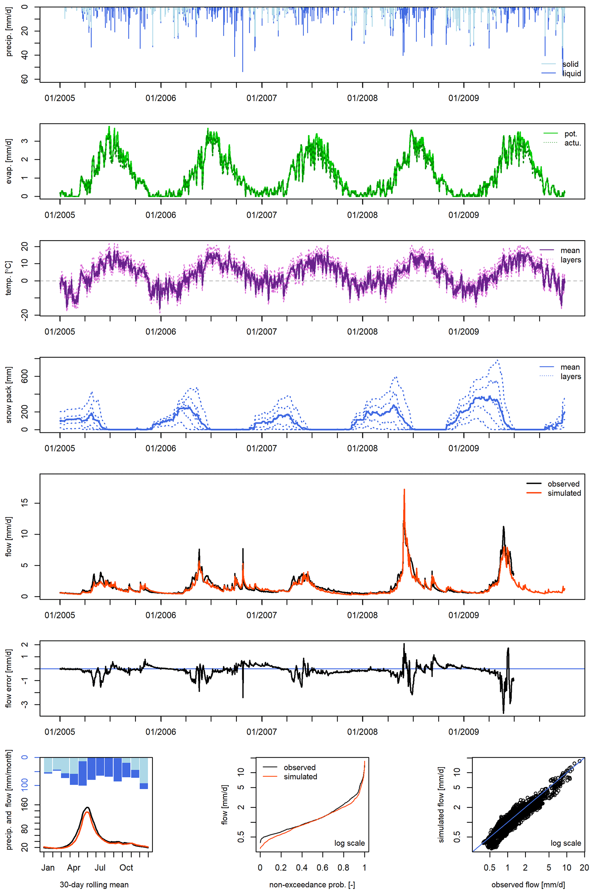
Figure A1 Example of plots enabled by the airGR package. This example was generated by using one of the data sets included in the package and simulations made with the GR4J-CemaNeige hydrological model. From top to bottom: solid and liquid precipitation time series (TS); potential and actual evapotranspiration TS; temperature TS for each layer; snow pack TS for each layer; simulated and observed hydrographs; flow error (or residuals). On the bottom line from left to right: interannual monthly median; cumulative frequency; bias. The hydrographs and the flow error charts can be visualised with a log scale.

Figure A2 Example of a plot enabled by the dynatopmodel package. This example was generated by using the data set included in the package. This figure combines plots of actual evapotranspiration time series, precipitation time series and simulated and observed hydrograph.

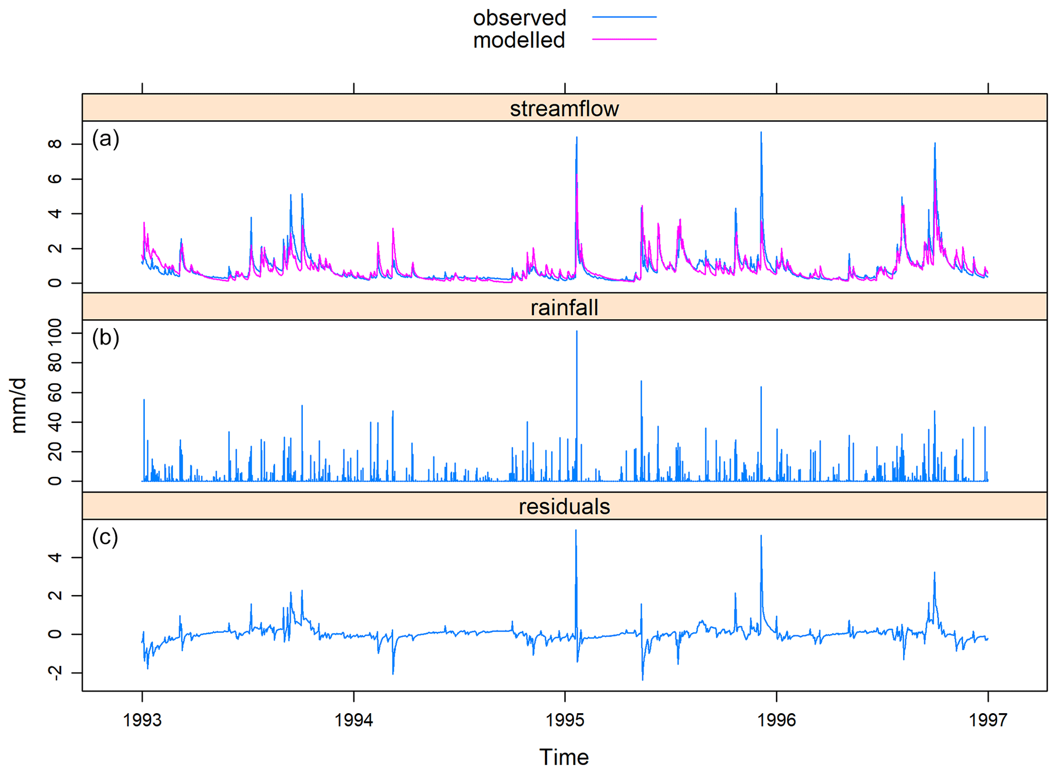
Figure A3 Example of plots enabled by the hydromad package. This example was generated by using one of the data sets included in the package and simulations with the IHACRES-CMD model. From top to bottom: observed and simulated hydrographs; precipitation time series; flow error (or residuals). These charts can be visualised with a log scale.

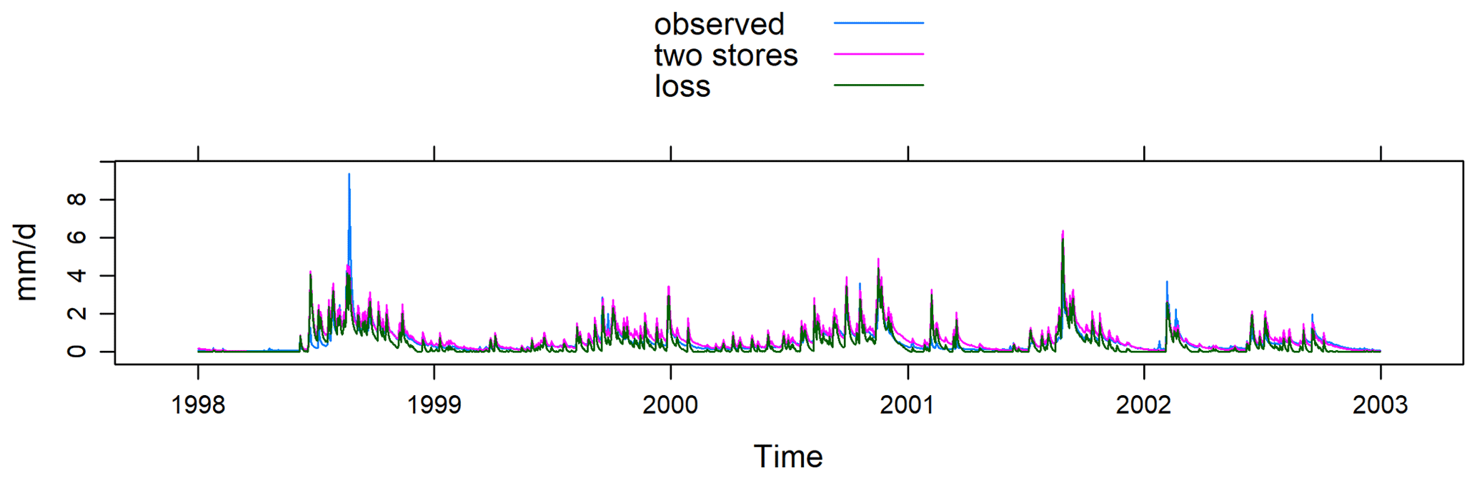
Figure A4 Example plots of simulation results from two model configurations enabled by the hydromad package. This example was generated by using one of the data sets included in the package and simulations with the IHACRES-CMD model. This chart can be visualised with a log scale.

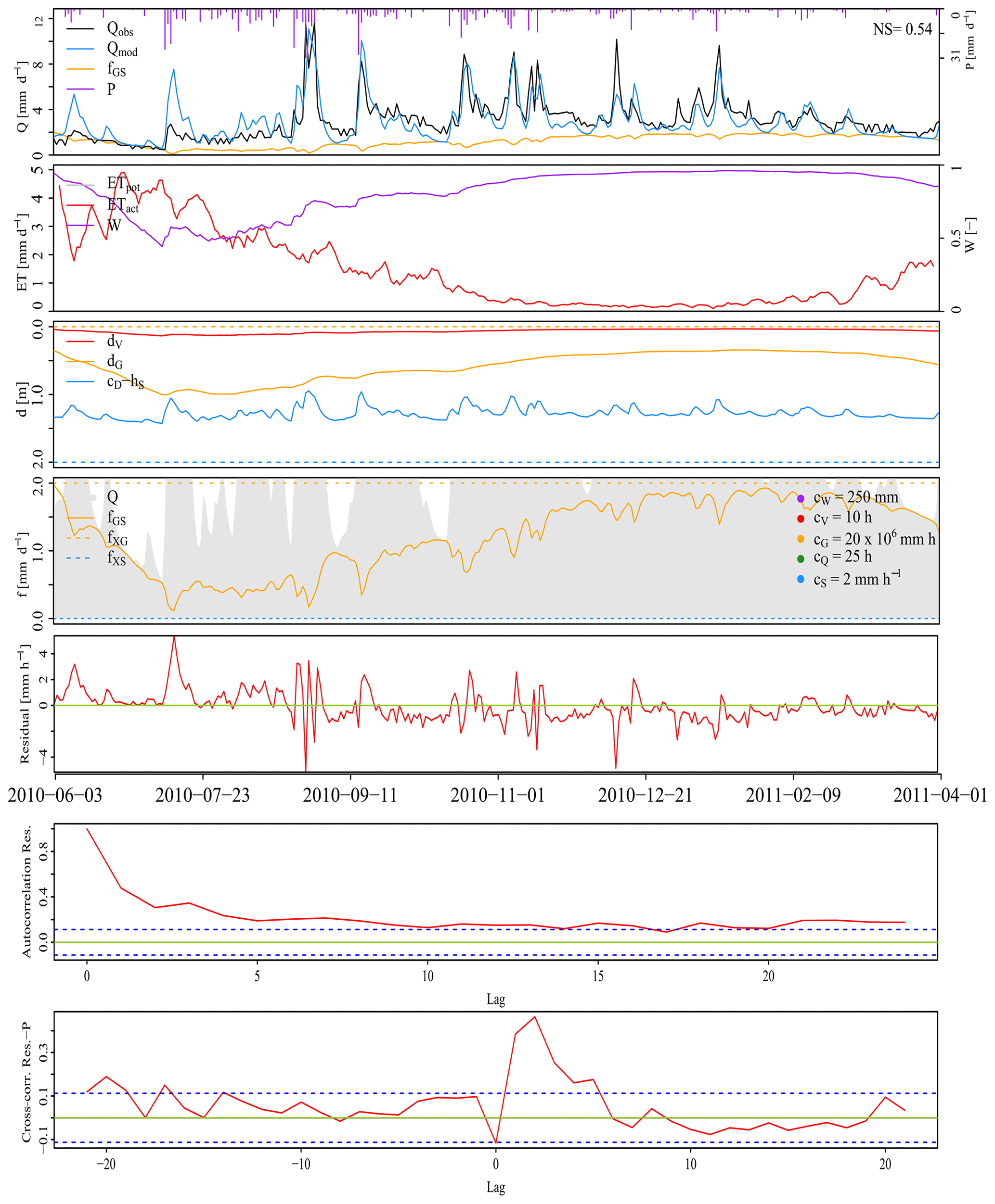
Figure A5 Example of plots enabled by the WALRUS package. This example was generated by using one of the data sets included in the package and simulations with the WALRUS model. From top to bottom: precipitation time series (TS), simulated hydrograph, observed hydrograph and modelled groundwater drainage; potential evapotranspiration TS, modelled actual evapotranspiration TS, wetness index TS; soil reservoir level TS and surface reservoir level TS; seepage TS and surface water supply or extraction TS; flow error (or residuals); autocorrelation of residuals; cross-correlation between residuals and precipitation.

Appendix B: Graphical user interfaces

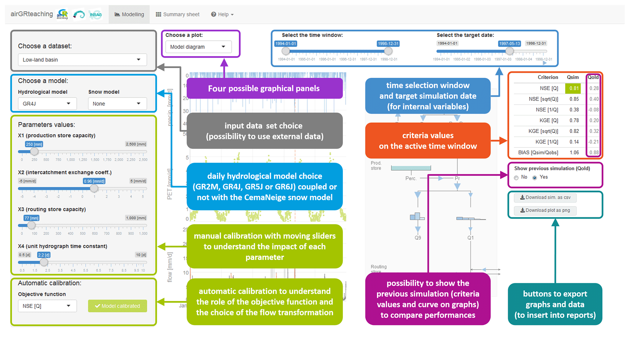
Figure B1 Graphical user interface of airGR using the airGRteaching package and describing the different functionalities.

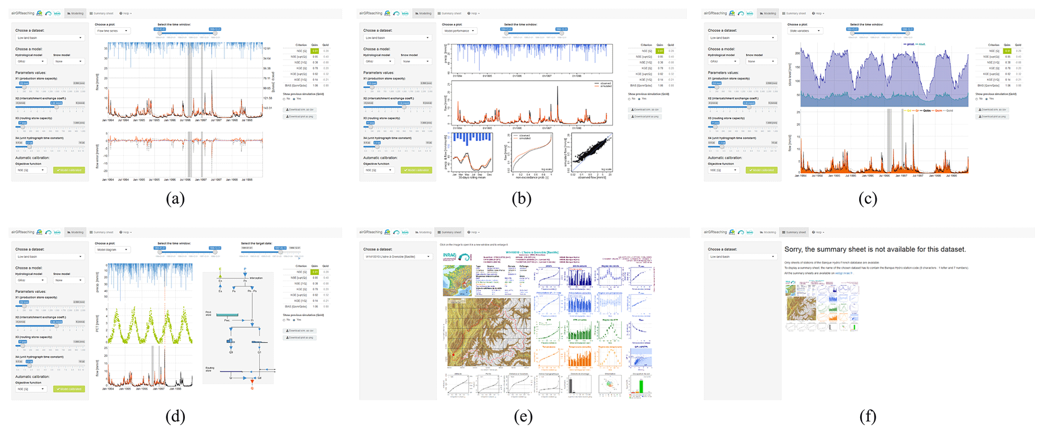
Figure B2 Graphical user interface of airGR using the airGRteaching package. (a) The time series of flow error (bottom graphic) and simulated and observed hydrographs (top graphic). (b) Performance graphics. (c) The time series of runoff components (bottom graphic) and reservoir levels (top graphic). (d) The interactive model diagram (right graphic) and the time series (left graphic) of precipitation, potential evapotranspiration, simulated flows and observed flows (from top to bottom). (e) Several hydrometeorological characteristics of the selected catchment. (f) When catchment characteristics are not available.

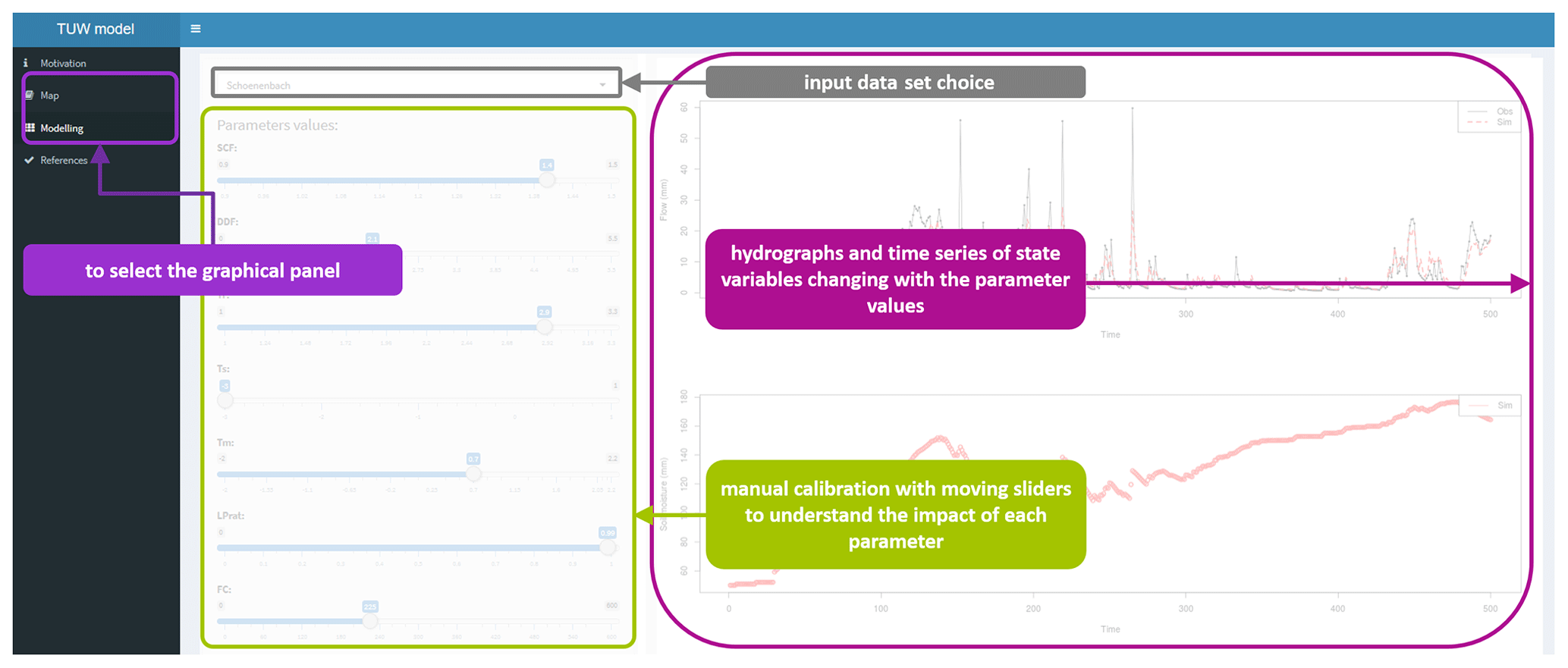
Figure B3 Graphical user interface of the TUWmodel package, with a diagram describing the different functionalities.

Figure B4 Graphical user interface of the TUWmodel package. (a) Tab where users can adjust the model parameters and see the impacts on (from top to bottom) the simulated hydrograph compared to the observed hydrograph, the simulated time series of soil moisture, the simulated time series of melt, and the simulated time series of snow water equivalent. (b) Tab where users can visualise the localisation of the five available catchment data sets on a map of Austria.