the Creative Commons Attribution 4.0 License.
the Creative Commons Attribution 4.0 License.
 | 21 Jan 2021
At which timescale does the complementary principle perform best in evaporation estimation?
Liming Wang
Songjun Han
The complementary principle has been widely used to estimate evaporation under different conditions. However, it remains unclear at which timescale the complementary principle performs best. In this study, evaporation estimations were conducted at 88 eddy covariance (EC) monitoring sites at multiple timescales (daily, weekly, monthly, and yearly) by using sigmoid and polynomial generalized complementary functions. The results indicate that the generalized complementary functions exhibit the highest skill in estimating evaporation at the monthly scale. The uncertainty analysis shows that this conclusion is not affected by ecosystem type or energy balance closure method. Through comparisons at multiple timescales, we found that the slight difference between the two generalized complementary functions only exists when the independent variable (x) in the functions approaches 1. The results differ for the two models at daily and weekly scales. However, such differences vanish at monthly and annual timescales, with few high x values occurring. This study demonstrates the applicability of generalized complementary functions across multiple timescales and provides a reference for choosing a suitable time step for evaporation estimations in relevant studies.
- Article
(5040 KB) - Full-text XML
-
Supplement
(315 KB) - BibTeX
- EndNote


Terrestrial evaporation (E), including soil evaporation, wet canopy evaporation, and plant transpiration, is one of the most important components in the global water cycle and energy balance (Wang and Dickinson, 2012). The evaporation process affects the atmosphere through a series of feedbacks involving humidity, temperature, and momentum (Brubaker and Entekhabi, 1996; Neelin et al., 1987; Shukla and Mintz, 1982). Quantifying evaporation is crucial for a deep understanding of water and energy interactions between the land surface and the atmosphere. Generally, meteorological studies focus on evaporation changes at hourly and daily scales; hydrological applications require evaporation data at weekly, monthly, or longer timescales (Morton, 1983); and climate change studies focus more on interannual variations. The observation of E can occur at different timescales. For example, the eddy covariance, lysimeter, and scintillometer can measure evaporation at the half-hour scale, and water balance methods can observe evaporation at monthly to yearly scales (Wang and Dickinson, 2012). However, in most situations, an observation is unavailable, and the estimation of E is necessary. There are several types of methods for evaporation estimations, for example, the Budyko-type methods (Budyko, 1974; Fu, 1981), the Penman-type methods (Penman, 1948; Monteith, 1965), and the complementary-type methods (Bouchet, 1963; Brutsaert and Stricker, 1979). The Budyko-type methods perform well at annual or longer timescales, and the Penman-type methods can be applied at hourly and daily scales, while the complementary-type methods are used at multiple timescales (Crago and Crowley, 2005; Han and Tian, 2018; Ma et al., 2019) without explicit consideration of the timescale issue.
Recently, the complementary principle, as one of the major types of E estimation methods, has drawn increasing attention because it can be implemented with standard meteorological data (radiation, wind speed, air temperature, and humidity) without complicated underlying surface properties. Based on the coupling between the land surface and the atmosphere, the complementary principle assumes that the limitation of the wetness state in the underlying surface on evaporation can be synthetically reflected by atmospheric wetness (Han and Tian, 2020). Bouchet (1963) first proposed the “complementary relationship” (CR), which suggested that apparent potential evaporation (Epa) and actual E depart from potential evaporation (Epo) in equal absolute values but opposite directions (). According to the advection–aridity approach (AA; Brutsaert and Stricker, 1979), Epa is formulated by Penman's (1948) equation (Epen), and Epo is formulated by Priestley and Taylor's (1972) equation (EPT). Subsequently, the CR was extended to a linear function with an asymmetric parameter (Brutsaert and Parlange, 1998). Further studies have found that the linear function underestimates E in arid environments and overestimates E in wet environments (Han et al., 2008; Hobbins et al., 2001; Qualls and Gultekin, 1997). To address this issue, Han et al. (2011, 2012) and Han and Tian (2018) proposed a sigmoid generalized complementary function (SGC; see Eq. 1 for details). As a modification to the AA approach, the SGC function illustrates the relationship between two dimensionless terms, E/Epen and Erad∕Epen, where Epen is Penman evaporation (Penman, 1948) andErad is the radiation term of Epen. The SGC function shows higher accuracy in estimating E (Han and Tian, 2018; Ma et al., 2015b; Zhou et al., 2020) and outperforms the linear functions, especially in dry desert regions and wet farmlands (Han et al., 2012). Obtaining the impetus from Han et al. (2012), Brutsaert (2015) proposed a quartic polynomial generalized complementary function (PGC; see Eq. 5 for details). The PGC function describes the relationship between E∕Epa and Epo∕Epa, where Epa and Epo are formulated in the manner of the AA approach. The PGC function has also been frequently used in recent years (Brutsaert et al., 2017; Hu et al., 2018; Liu et al., 2016; Zhang et al., 2017).
The prerequisite of the complementary principle is adequate feedback between the land surface and the atmosphere, which results in an equilibrium state. In this situation, the wetness condition of the land surface can be largely represented by the atmospheric conditions. Therefore, the timescales used in the complementary principle need to satisfy the adequate feedback assumption. However, this issue involves the complex processes of atmospheric horizontal and vertical motion, and these processes are difficult to explain theoretically. Morton (1983) noted this problem earlier and suggested that the complementary principle is not suitable for short timescales (e.g., less than 3 d), mainly because of the potential lag times associated with the response of energy and water vapor storage to disturbances in the atmospheric boundary layer. However, there is no solid evidence or theoretical identification to support this inference. The original complementary relationship and the AA function are not limited by applicable timescales. In the derivation of the advanced generalized complementary functions (SGC of Han and Tian, 2018, and PGC of Brutsaert, 2015), no specific timescale is defined. In practice, the complementary principle has been widely adopted to estimate E at multiple timescales, including hourly (Crago and Crowley, 2005; Parlange and Katul, 1992), daily (Han and Tian, 2018; Ma et al., 2015b), monthly (Ma et al., 2019; Brutsaert, 2020), and annual scales (Hobbins and Ramirez, 2004). The accuracy of the results has varied in different studies. Crago and Crowley (2005) found that the linear complementary function performs well in estimating E at small timescales of less than half an hour using the data from several well-known experimental projects (e.g., International Satellite Land Surface Climatology Project). The correlation coefficient between simulated E and observed E ranges from 0.87 to 0.92 in different experiments. The results of Ma et al. (2015b) indicated that the SGC function (root mean square error, RMSE = 0.39 mm d−1) performs well in estimating E in an alpine steppe region of the Tibetan Plateau at the daily scale. Han and Tian (2018) applied the SGC function to the daily data of 20 eddy covariance (EC) sites from FLUXNET and found that it performed well in estimating E, with a mean Nash–Sutcliffe efficiency (NSE) value of 0.66. Crago and Qualls (2018) evaluated the PGC function and their rescaled complementary functions using the weekly data of seven FLUXNET sites in Australia, and the results showed that all the functions performed adequately, with a correlation coefficient between simulated E and observed E of higher than 0.9. Ma et al. (2019) also validated an emendatory polynomial complementary function at the monthly scale, and the NSE values of 13 EC sites in China were higher than 0.72. At the annual scale, Zhou et al. (2020) found that the mean NSE of the SGC function was 0.28 for 15 catchments in the Loess Plateau. Since these results were derived with different functions under varied conditions, it is difficult to determine at which timescale the performance is the best, and it is more difficult to explain theoretically how long the land–atmosphere feedback needs to achieve equilibrium.
In previous studies, the model validations were mostly completed at the daily scale (Brutsaert, 2017; Han and Tian, 2018; Wang et al., 2020), and the datasets of evaporation estimation were often established at the monthly scale (Ma et al., 2019; Brutsaert et al., 2020). However, each study only focused on a single timescale. In this study, we assessed the performance of the complementary functions in evaporation estimation at multiple timescales (daily, weekly, monthly, and yearly). The assessment was carried out at 88 EC monitoring sites with > 5-year-long observation records. In view of the fact that the complementary principle has developed to the nonlinear generalized forms, we selected two nonlinear complementary functions in the literature, i.e., the SGC function (Han et al., 2012, 2018) and the PGC function (Brutsaert, 2015). The key parameters of the complementary functions need to be determined by calibration. We chose the uniform database and the uniform parameter calibration methods for the optimization of the two complementary functions. We aimed to determine the most suitable timescale for the complementary functions through a comparison of the performances at different timescales. It is important for not only a deep understanding of the application of the complementary principle but also time step selection in evaporation database establishment and evaporation trend analysis.
This paper is organized as follows: Sect. 1 briefly describes the development of the complementary theory and our motivations to investigate the timescale issue. Section 2 describes the two functions, the parameter calibration method, and the data sources and processing. Section 3 shows and discusses the performance of the complementary functions at multiple timescales, the dependence of the key parameters on timescales, and the uncertainties in the analysis. The conclusions are given in Sect. 4.
2.1 Sigmoid generalized complementary function
Han et al. (2012, 2018) proposed a generalized form of the complementary function that expresses E∕Epen as a sigmoid function (SGC) of Erad∕Epen:
where xmax corresponds to the certain maximum value of x under extremely wet environments, and xmin corresponds to the certain minimum value of x under extremely arid environments. In this study, xmax and xmin were set as 1 and 0, respectively, for convenience. The Epen term is defined by Penman's equation (Penman, 1948, 1950), which can be expressed as
where Δ (kPa C−1) is the slope of the saturation vapor curve at air temperature; Rn is the net radiation; G is the ground heat flux; γ (kPa C−1) is a psychrometric constant; ρ is the air density; cp is the specific heat; κ= 0.4 is the von Karman constant; u is the wind speed at measurement height; and ea are the saturated and actual vapor pressures of air, respectively; z is the measurement height (Table S1); d0 is the displacement height; z0m and z0v are the roughness lengths for momentum and water vapor, respectively, which are estimated from the canopy height (hc; Table S1), d0=0.67hc, z0m=0.123hc, and z0v=0.1z0m (Monin and Obukhov, 1954; Allen et al., 1998). Erad is the radiation term of Penman evaporation:
The two parameters m and n of Eq. (1) can be determined by the Priestley–Taylor coefficient α and the asymmetric parameter b (Han and Tian, 2018).
where x0.5 is a variable that corresponds to y= 0.5 and equals .
2.2 Polynomial generalized complementary function
Brutsaert (2015) proposed the polynomial generalized complementary (PGC) function, which describes the relationship between E/Epa and Epo∕Epa. We uniformed the independent variable as Erad∕Epen to compare the two functions conveniently, and the polynomial function can be expressed as
where c is an adjustable parameter. When c= 0, Eq. (5) reduces to
2.3 Parameter optimization method
Typically, α has a default value of 1.26 (Priestley and Taylor, 1972). Since some studies have shown that a constant α may cause illogical results and biases in estimating E, it is suggested to specify α for diverse scenarios (Hobbins et al., 2001; Ma et al., 2015a; Sugita et al., 2001; Szilagyi, 2007). According to the complementary principle, under wet conditions, E is close to Epen and the Priestley–Taylor's evaporation (EPT=αErad). Specifically, when E∕Epen is larger than a threshold (0.9 is commonly adopted), EPT can be considered to be approximately equal to the observed E; thus, α can be calculated by E∕Erad (Kahler and Brutsaert, 2006; Ma et al., 2015a). In this study, α was calculated using this method based on the mean value of E∕Erad under wet conditions (E∕Epen > 0.9). When all the E∕Epen values are less than 0.9, α was set as the default value of 1.26. The key parameter b in SGC was calibrated by an optimization algorithm, with the objective function as the minimization of the mean absolute error (MAE) between the estimated E (by Eq. 1) and the observed E. Similarly, the key parameter c in PGC was calibrated by an optimization algorithm, with the objective function as the minimization of the MAE between the estimated E (by Eq. 5) and the observed E. Since we used the optimization algorithm to determine the parameter b in the SGC function, it is a fair choice to use the optimal c value instead of a constant value (c=0) in the PGC function.
To make the model parsimonious, we gave one value for the parameters (α, b and c) at each site for every different timescale. If the parameter was alterable, for example, it was month-dependent, and we would have to calibrate 12 parameters instead of one value for the whole study period. The purpose of this study is to determine the most suitable timescale for the complementary functions, and the variances of the key parameter within a timescale will introduce extra uncertainties. The accuracy will increase when an alterable parameter (that means a higher number of parameters) is used; however, the probability of overfitting risk will increase at the same time. In addition, in comparison to a group of parameters, a general representation of the parameter is more helpful in detecting its overall trend as the change in the timescale.
2.4 Data sources and data processing
The eddy flux data analyzed in this study were obtained from the FLUXNET database (http://fluxnet.fluxdata.org; Baldocchi et al., 2001). Observations from a total of 88 sites around the world were analyzed. Detailed information on these sites is listed in Table S1. These sites were selected from the FLUXNET database because they have observations from a period longer than 5 years. The 88 sites include 11 IGBP (International Geosphere-Biosphere Programme) land cover classes: ENF, evergreen needleleaf forests (27 sites); EBF, evergreen broadleaf forests (8); DBF, deciduous broadleaf forests (13); MF, mixed forests (5); OSH, open shrublands (4); CSH, closed shrublands (1); WSA, woody savannas (3); SAV, savannas (4); GRA, grasslands (15); CRO, croplands (6); and WET, permanent wetlands (2). The climates of the 88 sites range from arid to humid. Among the 88 sites, 11 sites have mean annual precipitation levels lower than 200 mm, 47 sites have precipitation levels between 200–500 mm, and 30 sites have precipitation levels above 500 mm. A total of 11 sites are located in the Southern Hemisphere (i.e., Australia, Brazil, and South Africa), and the others are located in the Northern Hemisphere.
Variables including net radiation, sensible heat flux, latent heat flux, ground heat flux, wind speed, air temperature, air pressure, precipitation, relative humidity, and vapor pressure deficit were acquired from the daily, weekly, and monthly datasets on the FLUXNET website. We analyzed the observations in the growing seasons from April to September for the Northern Hemisphere and from October to March for the Southern Hemisphere. These study periods were selected to avoid the high biases caused by the low level of solar radiation or extremely low evaporation (≈ 0) during the non-growing season. The seasonal and annual data were acquired by averaging the monthly data of the growing seasons. Following Ershadi et al. (2014), the energy-residual-corrected latent heat fluxes were used, which means the residual term in the energy balance is attributed to the latent heat to force the energy balance closure. To investigate the influence of different residual correction methods, the Bowen ratio energy balance method was also adopted in the uncertainty analysis. In the Bowen ratio method, the residual term is attributed to sensible heat and latent heat by preserving the Bowen ratio (Twine et al., 2000). The latent heat, sensible heat, and available energy (Rn – G) are restricted to positive values (Han and Tian, 2018). The energy balance residual (W m−2) and energy balance closure ratio for each site are shown in Table S1.
The Nash–Sutcliffe efficiency (NSE; Legates and McCabe, 1999) is used to evaluate the efficiency of estimating E by the two generalized complementary functions:
where Eest (W m−2) is the estimated evaporation according to Eqs. (1) or (5), and is the mean value of E (W m−2).
3.1 Performance of the SGC function at multiple timescales
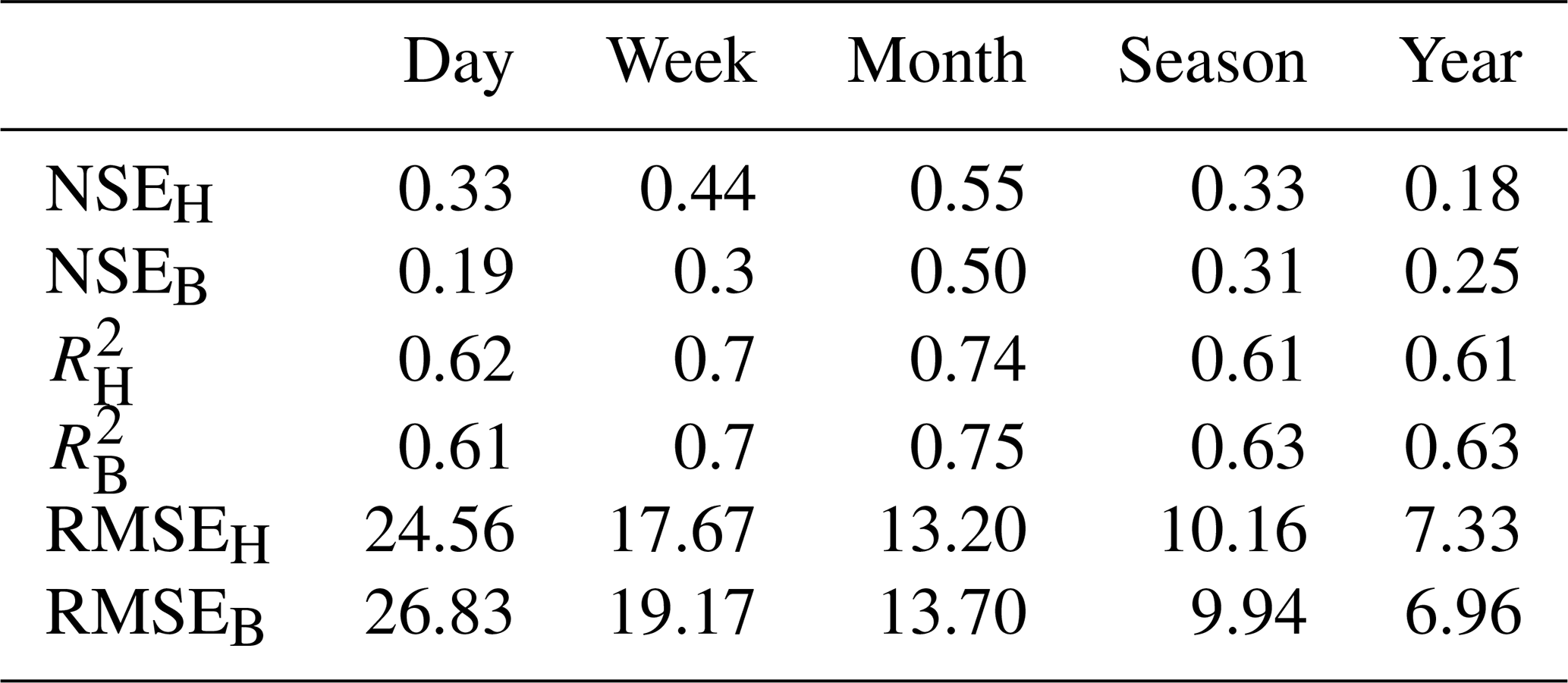
The relationship between the estimated Eest (site mean values) based on the SGC function (Eq. 1) and the observed E at the 88 sites at multiple timescales is shown in Fig. 1. The regression equations and determination coefficients (R2) were calculated using the site mean results. Each dot in Fig. 1 represents the site mean result averaged by daily (Fig. 1a), weekly (Fig. 1b), monthly (Fig. 1c), and yearly (Fig. 1d) results, and the total observation number is 88 (sites) at each timescale. Most of the results are near the 1:1 line, and all the regression slopes are close to 1 with high R2 (0.95–0.99), which means the sigmoid function exhibits a good performance in estimating E at multiple timescales. The evaluation merits show that the performance varies at each timescale. The NSE values of the SGC functions for each site at different timescales are listed in Table S2. For the 88 sites, nearly half of the sites (40) have the highest NSE at the monthly scale, 12 sites have the highest NSE at the daily scale, 13 sites have the highest NSE at the weekly scale, and 23 sites have the highest NSE at the annual scale. The mean results of NSEH, , and RMSEH (the subscript H corresponds to the sigmoid function proposed in Han and Tian, 2018) of these sites are shown in Table 1. represents the mean value averaged by the determination coefficients within each site. When the timescale changes from day to month, the mean NSEH increases from 0.33 to 0.55, and also increases from 0.61 to 0.75 (Table 1). However, they both decrease at the annual scale (NSEH= 0.18 and 0.61). These results indicate that the SGC function exhibits the highest skill at the monthly scale. We inferred that there is a trade-off between the random error and the number of observations. RMSEH values decrease from 24.56 W m−2 at the daily scale to 7.33 W m−2 at the annual scale, which means that the random error decreases as the timescale increases. At the same time, the fewer observations at the annual scale result in decreased variabilities of x and y, which affect the performance of the SGC function. On the other hand, Morton (1983) did not suggest using the complementary principle for short time intervals (e.g., less than 3 d), mainly considering the lag times associated with heat and water vapor change in the atmosphere, which may provide a possible inference for the weak performance at the daily scale.
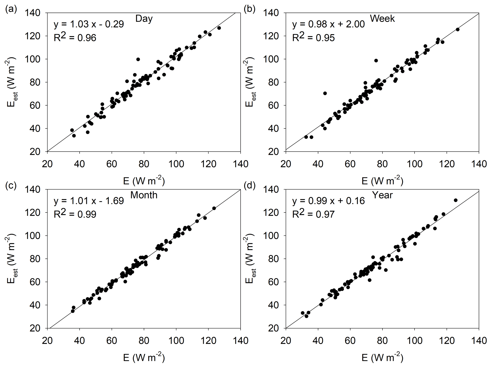
Figure 1The estimated evaporation based on the SGC function (Eq. 1) vs. the observed site mean evaporation at the daily scale (a), weekly scale (b), monthly scale (c), and yearly scale (d). Each dot represents the site mean result (N=88 in each panel). The regression equations and determination coefficients (R2) were calculated using the site mean results of the 88 EC sites.
Table 1The evaluation merits (NSE, R2, and RMSE in W m−2) of the two generalized complementary functions using the energy residual (ER) closure correction method. The subscripts H and B correspond to the SGC function proposed in Han and Tian (2018) and the PGC function proposed in Brutsaert (2015), respectively.
In previous studies, the SGC function was mainly applied at the daily scale. For example, the results of Ma et al. (2015b) in the alpine steppe region showed that the NSE of the sigmoid function is 0.73 at the daily scale, which is equal to our mean value in the grassland (0.73±0.08). The RMSE (11.06 W m−2) is smaller than ours (16.36±1.48 W m−2). The mean NSE of the 20 EC sites from FLUXNET is 0.66 at the daily scale in Han and Tian (2018), approximately 2 times the result in this study, and the RMSE (18.6 ± 0.94 W m−2) is lower than our mean result of 88 sites (24.56 ± 0.95 W m−2).
The SGC function for the five selected sites of different ecosystem types is shown in Fig. 2 to show the performance at multiple timescales (red lines in Fig. 2). These five EC monitoring sites were selected because they have long-term observations (> 10 years). The five sites include an evergreen needle forest (CA-TP1, Fig. 2a to d), a deciduous broad forest (US-UMB; Fig. 2e to h), a woody savanna (US-SRM; Figure 2i to l), a cropland (US-Ne2; Fig. 2m to p), and a grassland (US-Wkg; Fig. 2q to t). As observations decrease from the daily to the annual scale, the results converge on the middle part of the sigmoid curves and lie closer to the fitted lines. For some sites, the annual results concentrate on a narrow range with lower annual variabilities (e.g., Fig. 2h, l, and t). Generally, the key parameter (b) of the SGC function at these sites increases from the daily scale to the annual scale, which indicates that the sigmoid curves in the two-dimensional space of move upwards. A detailed discussion about the variation in the parameters is provided in Sect. 3.4.
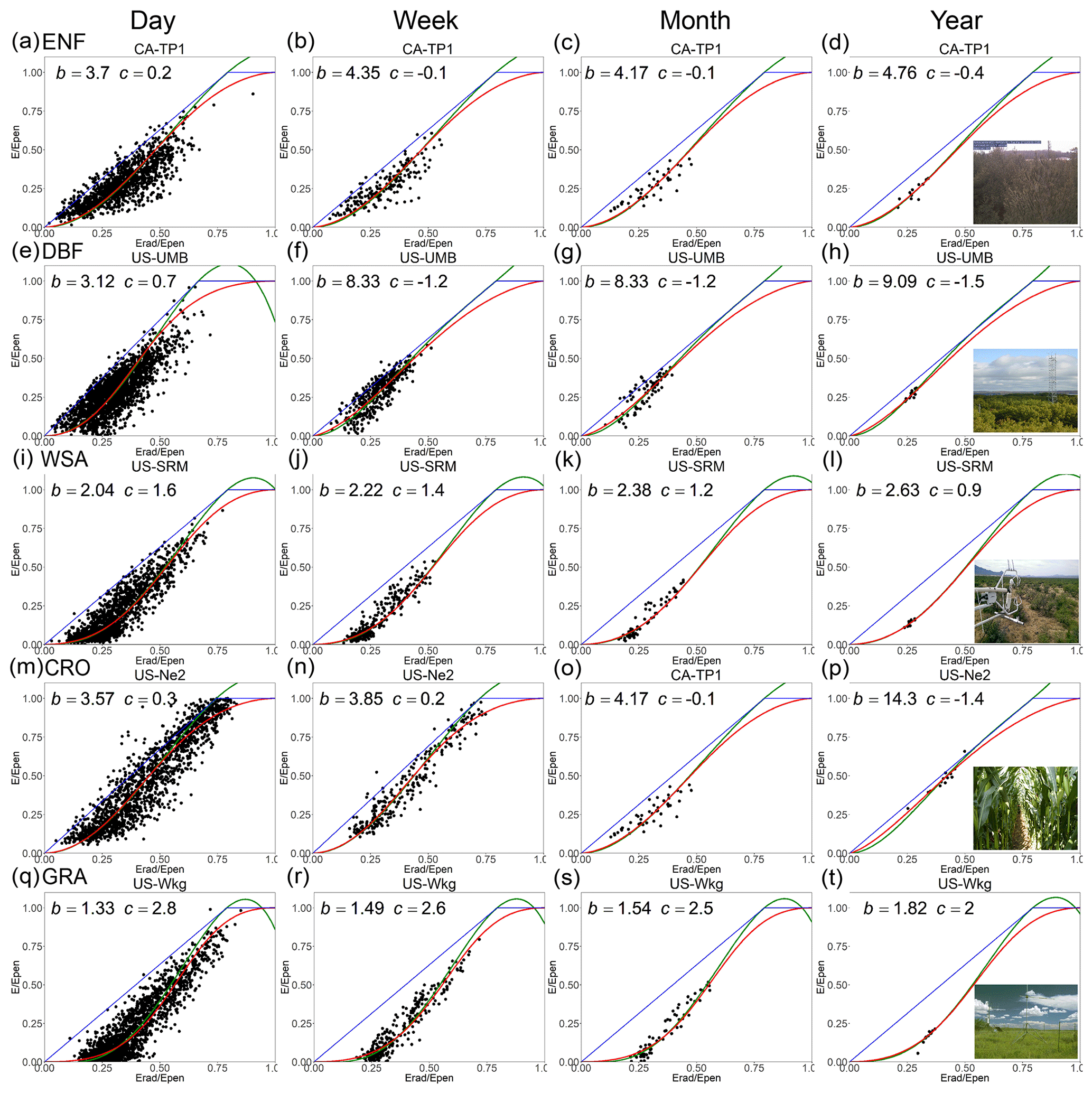
Figure 2Plots of E∕Epen with respect to Erad∕Epen for five selected sites at multiple timescales. The black dots represent the observations; the red lines represent the SGC function; the green lines represent the PGC function; the blue lines are the P–T and Penman boundary lines. ENF, evergreen needleleaf forests; DBF, deciduous broadleaf forests; WSA, woody savannas; CRO, croplands; GRA, grasslands.
3.2 Performance of the PGC function at multiple timescales
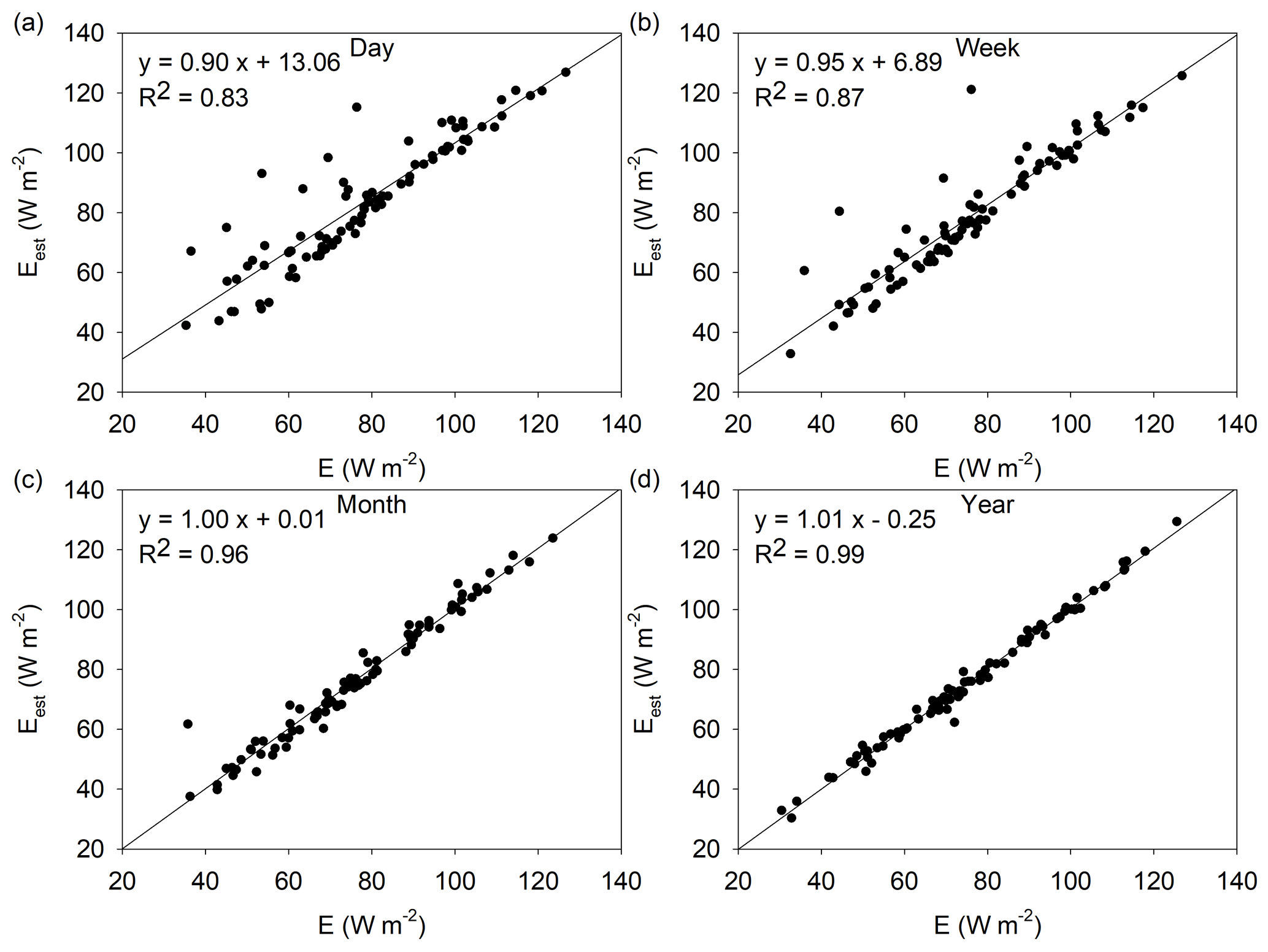
The relationship between the estimated Eest (site mean values) based on the PGC function (Eq. 5) and the observed E at the 88 sites at multiple timescales is shown in Fig. 3. The slopes of the regression increase from 0.9 to 1 as the timescale changes from day to month and further increase to 1.01 at the annual scale. The intercept terms decrease from 13.06 W m−2 at the daily scale to 0.01 W m−2 at the monthly scale and further decrease to −0.25 W m−2 at the annual scale. The R2 values increase from 0.83 to 0.99 as the timescale increases. These coefficients of the regression show that the PGC function exhibits the highest skill at the monthly scale. The NSE values of the PGC functions for each site at different timescales are listed in Table S2. For the 88 sites, 42 sites have the highest NSE at the monthly scale, 7 sites have the highest NSE at the daily scale, 14 sites have the highest NSE at the weekly scale, and 25 sites have the highest NSE at the annual scale. The mean values of NSEB, , and RMSEB (the subscript B corresponds to the polynomial function proposed in Brutsaert, 2015) of these sites are shown in Table 1. When the timescale changes from day to month, NSEB increases from 0.19 to 0.50, and increases from 0.61 to 0.75. They decrease at the annual scale (NSE = 0.25 and 0.63). Again, these evaluation merits indicate that the PGC function also exhibits the highest skill at the monthly scale, which is the same as for the SGC function.
The PGC function has been applied at multiple timescales in previous studies. Zhang et al. (2017) evaluated the performance of the PGC function in estimating evaporation at four EC flux sites located across Australia, and their results showed that the mean RMSE (24.67 W m−2) and R2 (0.65) are close to our results (RMSE = 26.83 ± 1.16 W m−2 and R2= 0.61) at the daily scale. In Crago and Qualls (2018), the mean RMSE of seven EC sites at the weekly scale was 20.6 W m−2, and the mean R2 was 0.81, which are close to our mean results (RMSE = 19.17 ± 0.95 W m−2 and R2= 0.7).
The PGC functions for the five selected sites are also shown in Fig. 2 (green lines). The fitted lines are almost the same as those of the SGC function in most situations when x is not too high. However, they diverge from each other when x becomes larger. Finally, y exceeds 1 when x is larger than 1∕α. Generally, the key parameter (c) of the PGC function at these sites decreases from the daily scale to the annual scale, which also indicates that the fitted curves move upwards.
3.3 Performance comparison of the SGC and PGC functions
The results from the 88 sites (Figs. 1, 3 and Table 1) show that the performances of the two functions are similar at monthly and annual timescales, while the SGC function performs slightly better than the PGC function at daily and weekly timescales. According to the results in Fig. 2, the two functions with calibrated parameters are approximately identical under non-humid environments, but their difference increases as x(Erad∕Epen) increases. We found that the values of α for all sites are greater than 1.0 in our study, which means that the PGC model cannot work properly under the condition of . At daily and weekly timescales, a substantial number of ecosystems can produce very high Erad∕Epen values. Specifically, 63 of the 88 sites have high Erad∕Epen values (x > 1∕α) at the daily scale, and 24 sites have high values at the weekly scale. However, there are only three sites with an x > 1∕α at the monthly scale, and no site has that value at the yearly scale. For the SGC function, in super-humid conditions, the upper part of the sigmoid curve is nearly flat and closer to the observations (e.g., Fig. 2a, m, and n). However, for the PGC function, theoretically, it cannot be applied when x is over 1∕α because the estimated Eest will be higher than Epen, which is illogical. Thus, the sigmoid function performs slightly better at daily and weekly timescales than the polynomial function. However, the difference vanishes at the monthly scale as few high Erad∕Epen values occur.
According to the results, the performance of the PGC function is more sensitive to the time step than that of the SGC function. On the one hand, the regression relationship between Eest and the observed E of the 88 sites shows that the performance of the SGC function remains more stable (Fig. 1), while the regression results of the PGC function have higher variation when the timescale changes (Fig. 3). On the other hand, the estimation merits (Table 1) further confirm the sensitivity of the PGC function. From the daily scale to the monthly scale, the increase in NSEH is 0.22, while the increase in NSEB is 0.31; RMSEH decreases by 11.36 W m−2 (46 %), and RMSEB decreases by 13.13 W m−2 (49 %). At the daily scale, quite a few ecosystems (63 of 88 sites) can experience frequent high Erad∕Epen (> 1∕α) values, and the PGC function does not have the ability to simulate E accurately in this situation (Eest > Epen), resulting in lower efficiency. We have carried out an additional analysis that adopts E=Epen for in the PGC function, and the resultant NSEB (0.19 vs. 0.19) and RMSEB (26.83 W m−2 vs. 26.68 W m−2) present very similar results. As the timescale increases, the results converge on the middle part of the fitted line, and the number of high x greatly decreases (Fig. 2). Thus, the efficiency of the PGC function obviously increases. This is the reason that the polynomial function acts more sensitively to the time step.
In addition, we found that the two complementary functions perform reasonably well at shorter timescales (i.e., day and week), with relatively high R2 values. Additionally, the estimations of site mean evaporation at shorter timescales are accurate (Figs. 1 and 3), especially for the SGC function. These results suggest that the generalized complementary functions have the ability to estimate evaporation accurately, even at shorter timescales.
3.4 Dependence of the key parameters of the SGC and PGC functions on timescales
The key parameters of the two complementary functions (b of the SGC function and c of the PGC function) vary at multiple timescales (Fig. 2). To explore their changes, the values of 1∕b and c at the 88 sites were averaged at each timescale. To take into account the situation in which b is equal to infinity, we used 1∕b instead of b in this analysis. Figure 4 shows the change in the two complementary functions with varied parameters at multiple timescales. The averaged 1∕b decreases from 0.45 ± 0.05 at the daily scale to 0.24 ± 0.03 at the annual scale (Fig. 4a), and the averaged c decreases from 0.98 ± 0.19 at the daily scale (Fig. 4b) to −0.37 ± 0.22 at the annual scale. The sign of c changes from positive to negative at the monthly scale.
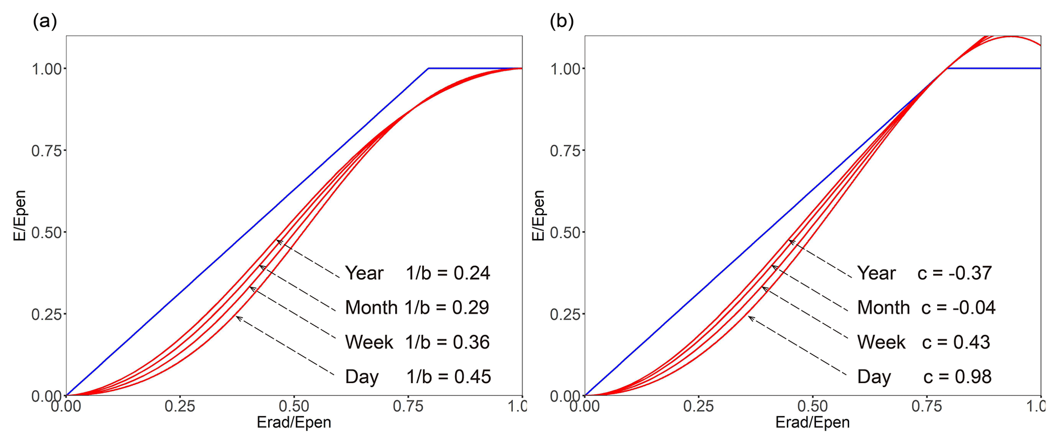
Figure 4Plots of the SGC Eq. (1) with α= 1.26 and varying 1∕b values at multiple timescales (a). Plots of the PGC Eq. (5) with α= 1.26 and varying c values at multiple timescales (b). The blue lines are the P–T and Penman boundary lines.
We show the histograms of 1∕b and c at multiple timescales in Figs. 5 and 6, respectively. At the daily scale, half of the 1∕b values are lower than 0.3, and the mean value is 0.45 ± 0.05. At the weekly scale, the peak of the distribution moves left, and almost half of the 1∕b values are lower than 0.2, with a mean value of 0.36 ± 0.04. At the monthly scale, the mean value is 0.29 ± 0.04, and the 1∕b values continue to decrease. At the annual scale, the mean value decreases to 0.24 ± 0.03, and 61 % of the 1∕b values are lower than 0.2. According to Fig. 6, at the daily scale, c follows a normal distribution (p value = 0.17, Kolmogorov–Smirnov test), with a mean value of 0.98 ± 0.21. Nearly 1∕3 of the c values are lower than 0. At the weekly scale, the center of the distribution moves left, with a mean value of 0.43 ± 0.24. Half of the c values are lower than 0. At the monthly scale, the mean value is −0.04 ± 0.23, and 58 % of the c values are lower than 0. At the annual scale, the mean value decreases to −0.37 ± 0.25, and 63 % of the c values are lower than 0. These results support our conclusion that 1∕b and c decrease as the timescale increases. Generally, the distribution of 1∕b and c also moves left within each ecosystem type according to Figs. 5 and 6.
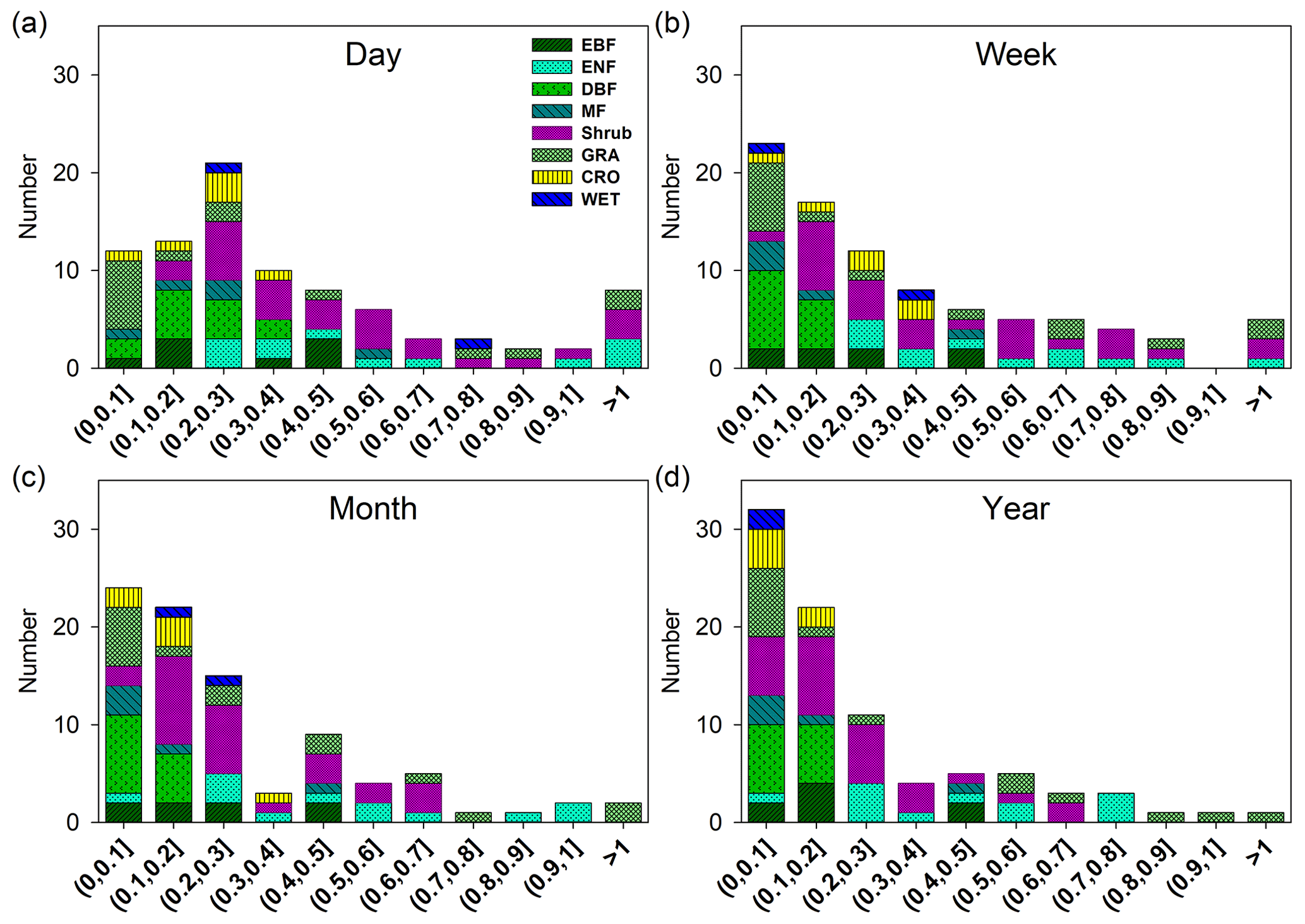
Figure 5Distribution of the key parameter 1∕b at the daily scale (a), weekly scale (b), monthly scale (c), and yearly scale (d). EBF, evergreen broadleaf forests (8); ENF, evergreen needleleaf forests (27); DBF, deciduous broadleaf forests (13); MF, mixed forests (5); shrub (12), closed shrubland, open shrublands, woody savannas, and savannas; GRA, grassland (15); CRO, croplands (6); WET, permanent wetlands (2).
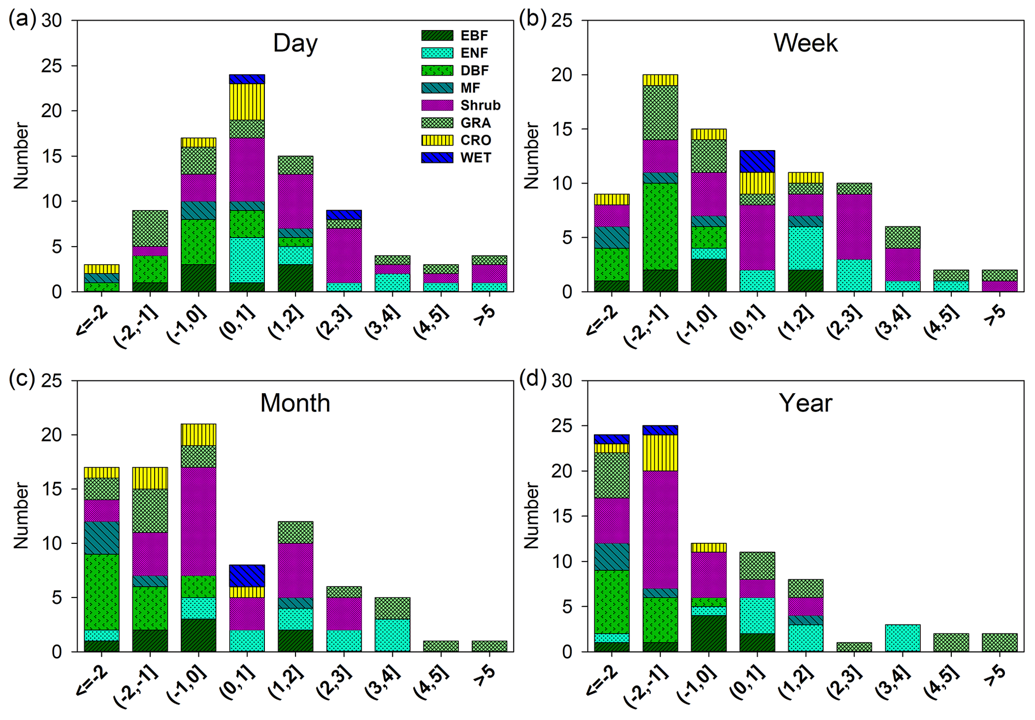
Figure 6Distribution of the key parameter c at the daily scale (a), weekly scale (b), monthly scale (c), and yearly scale (d). EBF, evergreen broadleaf forests (8); ENF, evergreen needleleaf forests (27); DBF, deciduous broadleaf forests (13); MF, mixed forests (5); shrub (12), closed shrubland, open shrublands, woody savannas, and savannas; GRA, grassland (15); CRO, croplands (6); WET, permanent wetlands (2).
The reduction in 1∕b and c indicates that the curves of the complementary functions move upwards as the timescale increases. Under non-humid conditions, the sigmoid function is a concave function, which means
where f is the concave function, and x1 and x2 represent any two values on the x axis. Since most of the results follow the fitted line, the averaged results of the longer time step will move upwards in the two-dimensional space of , as well the new fitted curve. Although under super humid conditions, the SGC function is a convex function, there are fewer data under this condition as the timescale increases, and the shape of this part is almost unchanged (Fig. 4a). For the PGC function, when x is in the range of 0 to 1∕α, most of it is a concave function. For example, in the situation where c is equal to 0, the second derivative is higher than 0 as long as x is lower than 2∕3.
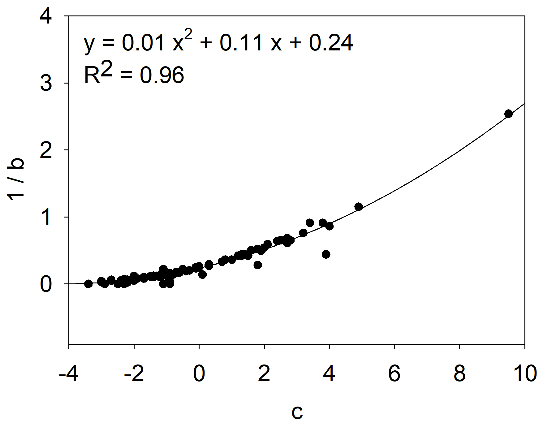
Furthermore, we found that the two key parameters b and c present a significant correlation, which provides additional evidence that the two functions can substitute each other in a sense. In other words, the two functions with calibrated parameters substantially provide similar descriptions of the distribution of the results in the state space (, ). They can covert to each other in most situations since the two functions are generally equivalent to the linear asymmetric function when x is neither excessively large nor excessively small. The relationship can be described as follows: 0.01, with R2 being higher than 0.96 at the monthly scale (Fig. 7). The relationship remains at other timescales with a slight difference in the regression coefficients. At the daily scale, when c is equal to 0, the corresponding b is equal to 4.5, which is the same as that of the theoretical derivation in Brutsaert (2015).
In this study, the physical meaning of the Priestley–Taylor coefficient α, which represents the ratio of EPT (the Priestley–Taylor evaporation) and Erad with the default value of 1.26 (Priestley and Taylor, 1972; Brutsaert and Stricker, 1979), was retained. This fundamental definition of α may result in a smaller range of Erad∕Epen in the PGC function. Liu et al. (2016) suggested that αe (the calibrated α with c=0) in the PGC function is only a weak analog of the Priestley–Taylor coefficient, and Brutsaert (2019) directly considered αe to be an adjustable parameter, which can be equal to or smaller than 1. We added the analysis that c is fixed to 0, and α is calibrated as αe. This analysis showed that the two methods provide similar results (mean RMSE = 14.99 W m−2 for αe vs. 16.67 W m−2 for α), and the conclusion of the timescale issue is consistent by adopting either α or αe in the analysis. The optimal αe has a significantly negative linear relationship with the optimal c, and the Pearson correlation coefficient is −0.8. This scenario suggests that calibrating either of the two parameters (αe and c) is equivalent (Han et al., 2012).
3.5 Uncertainty analysis
3.5.1 Influence of ecosystem types
The evaluation merits of the generalized complementary functions may differ among ecosystem types. However, our results show that such variation generally does not affect our conclusion that the complementary functions perform best at the monthly scale. We show the performance of the two functions at multiple timescales for each ecosystem type in Table S3. Generally, the SGC function and the PGC function perform best at the monthly scale in most ecosystem types (9 of 11), with the highest NSE and R2, which is consistent with the overall results. The exceptions include a closed shrubland site (CSH, N= 1) and evergreen broadleaf forests (EBF, N = 8), in which the complementary functions do not perform as well as in other ecosystem types. The CSH site (IT-Noe) has the highest NSEH (0.11) and NSEB (0.12) at the annual scale. In the EBF group, the highest NSEH (0.15) and NSEB (0.03) occur at the weekly scale, but the R2 values at the weekly scale ( 0.64; 0.62) and those at the monthly scale ( 0.62; 0.61) are similar. The RMSEs at the weekly scale are 14.95 W m−2 and 16.08 W m−2 for the sigmoid function and polynomial function, respectively, and those values at the monthly scale are 12.36 W m−2 (RMSEH) and 12.93 W m−2 (RMSEB). We inferred that the abnormal results of these two exceptions are related to the lower NSE values in these ecosystem types. The mean NSE values at multiple timescales of CSH (−0.75) and EBF (−0.66) are negative, while the values of the other ecosystem types are all positive.
3.5.2 Performance at the seasonal scale
In consideration of the substantial discrepancy between the monthly results and the annual results, we added an analysis at the seasonal scale, which is between the two time steps. The relationship between the estimated Eest (site mean values) and the observed E of the 88 sites at the seasonal scale is shown in Fig. S1. For the SGC function, the regression result at the seasonal scale is similar to that at the monthly scale (Figs. S1a and 1c). The values of NSEH (0.33), (0.61), and RMSEH (10.16 W m−2) at the seasonal scale are between the monthly results and the yearly results (Table 1). For the PGC functions, the regression result at the seasonal scale is extremely close to that at the yearly scale (Fig. S1b and 3d). The evaluation merits (NSEB = 0.31; 0.63; RMSEB= 9.94 W m−2) also range between the monthly results and the yearly results (Table 1). These results indicate that the decline in model efficiency has already occurred at the seasonal scale and support our conclusion that the complementary functions perform best at the monthly scale.
In addition, we also tested the influence of the different energy balance closure methods. The results based on both the energy residual (ER) closure correction (e.g., Ershadi et al., 2014; Han and Tian, 2018) and the Bowen ratio (BR) closure correction support our conclusion that the generalized complementary functions perform best at the monthly scale (Table S4).
In this study, evaporation estimations were assessed at 88 EC monitoring sites at multiple timescales (daily, weekly, monthly, and yearly) by using two generalized complementary functions (the SGC function and the PGC function). The performances of the complementary functions at multiple timescales were compared, and the variation in the key parameters at different timescales was explored. The main findings are summarized as follows:
-
The sigmoid and polynomial generalized complementary functions exhibit higher skill in estimating evaporation at the monthly scale than at the other evaluated scales. The highest evaluation merits were obtained at this timescale. The accuracy of the complementary functions highly depends on the calculation time step. The NSE increases from the daily scale (0.26, averaged by NSEH and NSEB) to the weekly scale (0.37) and monthly scale (0.53), while it decreases at the seasonal scale (0.32) and the annual scale (0.22). The regression parameters between estimated Eest and observed site mean E also support this conclusion for the PGC function. The variations among the different ecosystem types or between different energy balance closure methods generally have no effect on this conclusion. Further evaporation estimation studies with complementary functions can choose the monthly time step to achieve the most accurate results.
-
The SGC function and the PGC function are approximately identical under non-humid environments, while the SGC function performs better under super humid conditions implied by high values of x (> 1∕α) when the PGC function is theoretically useless (Eest > Epen). At daily and weekly timescales, a substantial number of ecosystems can experience frequent high x values, and thus, the SGC function performs slightly better than the PGC function at these timescales. However, both functions perform very similarly at monthly and annual timescales, with few high x values. In addition, the performance of the PGC function is more sensitive to the time step than that of the SGC function.
-
The key parameter b of the SGC function increases and the key parameter c of the PGC function decreases as the timescale increases. The value of 1∕b is a quadratic function of c, with a higher R2 (> 0.96). The relationship at the monthly scale can be described as . This relationship indicates that the two functions serve as substitutes to some extent.
In this study to determine the most suitable timescale for applying the complementary principle, the key parameters (b and c) were calibrated to achieve the best model performance at each timescale. Further studies on the prognostic application of the complementary principle could focus on the reasonable prediction of the key parameters, and with the predictable flexible parameters at different timescales, the complementary principle could be integrated into hydrological models to reduce the uncertainty associated with evaporation estimations.
All the data used in this study are from FLUXNET (http://fluxnet.fluxdata.org; U.S. Department of Energy, 2020; Baldocchi et al., 2001). The information for the EC data used in this study is listed in the Supplement. The intermediate data are available on request from the corresponding author (tianfq@mail.tsinghua.edu.cn).
The supplement related to this article is available online at: https://doi.org/10.5194/hess-25-375-2021-supplement.
SH and FT designed the experiments, and LW carried them out. LW developed the model code and performed the simulations. LW prepared the paper with contributions from all co-authors.
The authors declare that they have no conflict of interest.
We are grateful for the financial support from the National Science Foundation of China (NSFC 51825902, 51579249, 52079147), the Ministry of Science and Technology of the People's Republic of China (2016YFC0402701), and the State Key Laboratory of Simulation and Regulation of Water Cycle in River Basin, China Institute of Water Resources and Hydropower Research (SKL2020ZY06). We thank the scientists of FLUXNET (http://fluxnet.fluxdata.org) for their generous sharing of their eddy flux data. We are grateful to the reviewers and the editors who provided valuable comments and suggestions for this work.
This research has been supported by the National Science Foundation of China (grant nos. NSFC 51825902, 51579249, and 52079147), Ministry of Science and Technology of the People's Republic of China (grant no. 2016YFC0402701) and State Key Laboratory of Simulation and Regulation of Water Cycle in River Basin, China Institute of Water Resources and Hydropower Research (grant no. SKL2020ZY06).
This paper was edited by Marnik Vanclooster and reviewed by three anonymous referees.
Allen, R. G., Pereira, L. S., Raes, D., and Smith, M.: Crop evapotranspiration: Guidelines for computing crop water requirements, FAO irrigation and drainage paper No. 56, Food and Agricultural Organization of the UN, Rome, Italy, 1998.
Baldocchi, D., Falge, E., Gu, L., Olson, R., Hollinger, D., Running, S., Anthoni, P., Bernhofer, C., Davis, K., Evans, R., Fuentes, J., Goldstein, A., Katul, G., Law, B., Lee, X., Malhi, Y., Meyers, T., Munger, W., Oechel, W., Paw, K., Pilegaard, K., Schmid, H., Valentini, R., Verma, S., Vesala, T., Wilson, K., and Wofsy, S.: FLUXNET: A new tool to study the temporal and spatial variability of ecosystem-scale carbon dioxide, water vapor, and energy flux densities, B. Am. Meteorol. Soc., 82, 2415–2434, https://doi.org/10.1175/1520-0477(2001)082<2415:FANTTS>2.3.CO;2, 2001.
Bouchet, R. J.: Evapotranspiration réelle et potentielle, signification climatique, Int. Assoc. Hydrolog. Sci. Publ., 62, 134–142, 1963.
Brubaker, K. L. and Entekhabi, D.: Analysis of feedback mechanisms in land-atmosphere interaction, Water Resour. Res., 32, 1343–1357, https://doi.org/10.1029/96wr00005, 1996.
Brutsaert, W.: A generalized complementary principle with physical constraints for land-surface evaporation, Water Resour. Res., 51, 8087–8093, https://doi.org/10.1002/2015wr017720, 2015.
Brutsaert, W. and Parlange, M. B.: Hydrologic cycle explains the evaporation paradox, Nature, 396, p. 30, https://doi.org/10.1038/23845, 1998.
Brutsaert, W. and Stricker, H.: Advection-Aridity approach to estimate actual regional evapotranspiration, Water Resour. Res., 15, 443–450, https://doi.org/10.1029/WR015i002p00443, 1979.
Brutsaert, W., Li, W., Takahashi, A., Hiyama, T., Zhang, L., and Liu, W. Z.: Nonlinear advection-aridity method for landscape evaporation and its application during the growing season in the southern Loess Plateau of the Yellow River basin, Water Resour. Res., 53, 270–282, https://doi.org/10.1002/2016wr019472, 2017.
Brutsaert, W., Cheng, L., and Zhang, L.: Spatial distribution of global landscape evaporation in the early twenty first century by means of a generalized complementary approach, J. Hydrometeorol., 21, 287–298, https://doi.org/10.1175/JHM-D-19-0208.1, 2020.
Budyko, M. I.: Climate and Life, Academic Press, San Diego, CA, USA, 1974.
Crago, R. and Crowley, R.: Complementary relationships for near-instantaneous evaporation, J. Hydrol., 300, 199–211, https://doi.org/10.1016/j.jhydrol.2004.06.002, 2005.
Crago, R. D. and Qualls, R. J.: Evaluation of the generalized and rescaled complementary evaporation relationships, Water Resour. Res., 54, 8086–8102, https://doi.org/10.1029/2018wr023401, 2018.
Ershadi, A., McCabe, M. F., Evans, J. P., Chaney, N. W., and Wood, E. F.: Multi-site evaluation of terrestrial evaporation models using FLUXNET data, Agric. Forest Meteorol., 187, 46–61, https://doi.org/10.1016/j.agrformet.2013.11.008, 2014.
Fu, B. P.: On the calculation of the evaporation from land surface, Sci. Atmos. Sin., 5, 23–31, 1981 (in Chinese).
Han, S. and Tian, F.: A review of the complementary principle of evaporation: from the original linear relationship to generalized nonlinear functions, Hydrol. Earth Syst. Sci., 24, 2269–2285, https://doi.org/10.5194/hess-24-2269-2020, 2020.
Han, S. J., Hu, H. P., and Tian, F. Q.: Evaluating the Advection-Aridity model of evaporation using data from field-sized surfaces of HEIFE, IAHS Publ., 322, 9–14, 2008.
Han, S. J., Hu, H. P., Yang, D. W., and Tian, F. Q.: A complementary relationship evaporation model referring to the Granger model and the advection-aridity model, Hydrol. Process., 25, 2094–2101, https://doi.org/10.1002/hyp.7960, 2011.
Han, S. J., Hu, H. P., and Tian, F. Q.: A nonlinear function approach for the normalized complementary relationship evaporation model, Hydrol. Process., 26, 3973–3981, https://doi.org/10.1002/hyp.8414, 2012.
Han, S. J. and Tian, F. Q.: Derivation of a sigmoid generalized complementary function for evaporation with physical constraints, Water Resour. Res., 54, 5050–5068, https://doi.org/10.1029/2017wr021755, 2018.
Han, S. and Tian, F.: A review of the complementary principle of evaporation: from the original linear relationship to generalized nonlinear functions, Hydrol. Earth Syst. Sci., 24, 2269–2285, https://doi.org/10.5194/hess-24-2269-2020, 2020.
Hobbins, M. T. and Ramirez, J. A.: Trends in pan evaporation and actual evapotranspiration across the conterminous US: Paradoxical or complementary?, Geophys. Res. Lett. 31, 405–407, https://doi.org/10.1029/2004GL019846, 2004.
Hobbins, M. T., Ramirez, J. A., and Brown, T. C.: The complementary relationship in estimation of regional evapotranspiration: An enhanced Advection-Aridity model, Water Resour. Res., 37, 1389–1403, https://doi.org/10.1029/2000wr900359, 2001.
Hu, Z. Y., Wang, G. X., Sun, X. Y., Zhu, M. Z., Song, C. L., Huang, K. W., and Chen, X. P.: Spatial-temporal patterns of evapotranspiration along an elevation gradient on Mount Gongga, Southwest China, Water Resour. Res., 54, 4180–4192, https://doi.org/10.1029/2018wr022645, 2018.
Kahler, D. M. and Brutsaert, W.: Complementary relationship between daily evaporation in the environment and pan evaporation, Water Resour. Res., 42, W05413, https://doi.org/10.1029/2005WR004541, 2006.
Legates, D. R. and Mccabe, G. J.: Evaluating the use of “goodness-of-fit” Measures in hydrologic and hydroclimatic model validation, Water Resour. Res., 35, 233–241, https://doi.org/10.1029/1998wr900018, 1999.
Liu, X. M., Liu, C. M., and Brutsaert, W.: Regional evaporation estimates in the eastern monsoon region of China: Assessment of a nonlinear formulation of the complementary principle, Water Resour. Res., 52, 9511–9521, https://doi.org/10.1002/2016wr019340, 2016.
Ma, N., Zhang, Y. S., Szilagyi, J., Guo, Y. H., Zhai, J. Q., and Gao, H. F.: Evaluating the complementary relationship of evapotranspiration in the alpine steppe of the Tibetan Plateau, Water Resour. Res., 51, 1069–1083, https://doi.org/10.1002/2014wr015493, 2015a.
Ma, N., Zhang, Y. S., Xu, C. Y., and Szilagyi, J.: Modeling actual evapotranspiration with routine meteorological variables in the data-scarce region of the Tibetan Plateau: Comparisons and implications, J. Geophys. Res.-Biogeo., 120, 1638–1657, https://doi.org/10.1002/2015jg003006, 2015b.
Ma, N., Szilagyi, J., Zhang, Y., and Liu, W.: Complementary relationship-based modeling of terrestrial evapotranspiration across China during 1982–2012: Validations and spatiotemporal analyses, J. Geophys. Res.-Atmos., 124, 4326–4351, https://doi.org/10.1029/2018JD029850, 2019.
Monin, A. and Obukhov, A.: Basic laws of turbulent mixing in the surface layer of the atmosphere, Contrib. Geophys. Inst. Acad. Sci. USSR, 151, e187, https://gibbs.science/efd/handouts/monin_obukhov_1954.pdf (last access: 12 July 2020), 1954.
Monteith, J. L.: Evaporation and environment, in: Symposium of the Society of Experimental Biology, Cambridge, UK, 1 January 1965, PMID: 5321565, 19, 205–234, 1965.
Morton, F. I.: Operational estimates of areal evapo-transpiration and their significance to the science and practice of hydrology, J. Hydrol., 66, 1–76, https://doi.org/10.1016/0022-1694(83)90177-4, 1983.
Neelin, J. D., Held, I. M., and Cook, K. H.: Evaporation-wind feedback and low-frequency variability in the tropical atmosphere, J. Atmos. Sci., 44, 2341–2348, https://doi.org/10.1175/1520-0469(1987)044<2341:Ewfalf>2.0.Co;2, 1987.
Parlange, M. B. and Katul, G. G.: An advection-aridity evaporation model, Water Resour. Res., 28, 127–132, https://doi.org/10.1029/91WR02482, 1992.
Penman, H. L.: Natural evaporation from open water, bare soil and grass, Proc. R. Soc. Lond. A., 193, 120–145, https://doi.org/10.1098/rspa.1948.0037, 1948.
Penman, H. L.: The dependence of transpiration on weather and soil conditions, J. Soil Sci., 1, 74–89, https://doi.org/10.1111/j.1365-2389.1950.tb00720.x, 1950.
Priestley, C. H. B. and Taylor, R. J.: On the assessment of surface heat-flux and evaporation using large-scale parameters, Mon. Weather Rev., 100, 81–92, https://doi.org/10.1175/1520-0493(1972)100<0081:Otaosh>2.3.Co;2, 1972.
Qualls, R. J. and Gultekin, H.: Influence of components of the advection-aridity approach on evapotranspiration estimation, J. Hydrol., 199, 3–12, https://doi.org/10.1016/S0022-1694(96)03314-8, 1997.
Shukla, J. and Mintz, Y.: Influence of land-surface evapo-transpiration on the earths climate, Science, 215, 1498–1501, https://doi.org/10.1126/science.215.4539.1498, 1982.
Sugita, M., Usui, J., Tamagawa, I., and Kaihotsu, I.: Complementary relationship with a convective boundary layer model to estimate regional evaporation, Water Resour. Res., 37, 353–365, https://doi.org/10.1029/2000wr900299, 2001.
Szilagyi, J.: On the inherent asymmetric nature of the complementary relationship of evaporation, Geophys. Res. Lett., 34, L02405, https://doi.org/10.1029/2006gl028708, 2007.
Twine, T. E., Kustas, W. P., Norman, J. M., Cook, D. R., Houser, P., Meyers, T. P., and Wesely, M. L.: Correcting eddy-covariance flux underestimates over a grassland, Agr. Forest Meteorol., 103, 279–300, https://doi.org/10.1016/S0168-1923(00)00123-4, 2000.
U.S. Department of Energy: FLUXNET2015, http://fluxnet.fluxdata.org, 15 Fenriaru 2020.
Wang, K. C. and Dickinson, R. E.: A review of global terrestrial evapotranspiration: observation, modeling, climatology, and climatic variability, Rev. Geophys., 50, 2011RG000373, https://doi.org/10.1029/2011rg000373, 2012.
Wang, L. M., Tian, F. Q., Han, S. J., and Wei, Z. W.: Determinants of the asymmetric parameter in the generalized complementary principle of evaporation, Water Resour. Res, 56, e2019WR026570, https://doi.org/10.1029/2019WR026570, 2020.
Zhang, L., Cheng, L., and Brutsaert, W.: Estimation of land surface evaporation using a generalized nonlinear complementary relationship, J. Geophys. Res.-Atmos., 122, 1475–1487, https://doi.org/10.1002/2016jd025936, 2017.
Zhou, H., Han, S., and Liu, W.: Evaluation of two generalized complementary functions for annual evaporation estimation on the loess plateau, China, J. Hydrol., 587, 124980, https://doi.org/10.1016/j.jhydrol.2020.124980, 2020.