the Creative Commons Attribution 4.0 License.
the Creative Commons Attribution 4.0 License.
 | 01 Jul 2021
Quantifying floodwater impacts on a lake water budget via volume-dependent transient stable isotope mass balance
Janie Masse-Dufresne
Florent Barbecot
Paul Baudron
John Gibson
Isotope mass balance models have undergone significant developments in the last decade, demonstrating their utility for assessing the spatial and temporal variability in hydrological processes and revealing significant value for baseline assessment in remote and/or flood-affected settings where direct measurement of surface water fluxes to lakes (i.e. stream gauging) are difficult to perform. In this study, we demonstrate that isotopic mass balance modelling can be used to provide evidence of the relative importance of direct floodwater inputs and temporary subsurface storage of floodwater at ungauged lake systems. A volume-dependent transient isotopic mass balance model was developed for an artificial lake (named lake A) in southern Quebec (Canada). This lake typically receives substantial floodwater inputs during the spring freshet period as an ephemeral hydraulic connection with a 150 000 km2 large watershed is established. First-order water flux estimates to lake A allow for impacts of floodwater inputs to be highlighted within the annual water budget. The isotopic mass balance model has revealed that groundwater and surface water inputs account for 60 %–71 % and 39 %–28 % of the total annual water inputs to lake A, respectively, which demonstrates an inherent dependence of the lake on groundwater. However, when considering the potential temporary subsurface storage of floodwater, the partitioning between groundwater and surface water inputs tends to equalize, and the lake A water budget is found to be more resilient to groundwater quantity and quality changes. Our findings suggest not only that floodwater fluxes to lake A have an impact on its dynamics during springtime but also significantly influence its long-term water balance and help to inform, understand, and predict future water quality variations. From a global perspective, this knowledge is useful for establishing regional-scale management strategies for maintaining water quality at flood-affected lakes, for predicting the response of artificial recharge systems in such settings, and for mitigating impacts due to land use and climate changes.
- Article
(3824 KB) - Full-text XML
- BibTeX
- EndNote


Lakes are complex ecosystems which play a valuable economic, social, and environmental role within watersheds (Kløve et al., 2011). In fact, lacustrine ecosystems can provide a number of ecosystem services, such as biodiversity, water supply, recreation and tourism, fisheries, and sequestration of nutrients (Schallenberg et al., 2013). The actual benefits that can be provided by lakes depend on the water quality, and poor resilience to water quality changes can lead to benefit losses (Mueller et al., 2016). Globally, the quantity and quality of groundwater and surface water resources are known to be affected by land use (Baudron et al., 2013; Cunha et al., 2016; Lerner and Harris, 2009; Scanlon et al., 2005) and climate changes (Delpla et al., 2009). As both surface water and groundwater contribute to lake water balances (Rosenberry et al., 2015), changes that affect the surface water/groundwater apportionment can potentially modify or threaten lake water quality (Jeppesen et al., 2014). Understanding hydrological processes in lakes can help to depict the vulnerability and/or resilience of a lake to pollution (Rosen, 2015) and to invasive species (Walsh et al., 2016) and, thus, secure water quantity and quality over time for drinking water production purposes (Herczeg et al., 2003). In Quebec (Canada), there are an important number of municipal wells that receive contributions from surface water resources (i.e. lakes or rivers) and are, thus, performing unintentional (Patenaude et al., 2020) or intentional (Masse-Dufresne et al., 2019, 2021) bank filtration.
Over the past few decades, significant developments have been made in the application of isotope mass balance models for assessing the spatial and temporal variability in hydrological processes in lakes, most notably the quantification of groundwater and evaporative fluxes (Herczeg et al., 2003; Bocanegra et al., 2013; Gibson et al., 2016; Arnoux et al., 2017b). In remote environments, such as in northern Canada, the application of isotopic methods is particularly convenient as direct measurements of surface water and groundwater fluxes is time-consuming, expensive, and difficult (Welch et al., 2018). Isotopic mass balance models can notably be applied to ungauged lake systems to efficiently characterize the impacts of floods on water apportionment (Haig et al., 2020). While isotopic frameworks were successfully used to assess the relative importance of floodwater inputs to lakes (Turner et al., 2010; Brock et al., 2007), no attempt was made to evaluate the timing of the floodwater inputs and to differentiate between the role of (i) direct floodwater inputs and (ii) temporary subsurface storage of floodwater on a lake's annual water budget. In this study, direct inputs refer to the floodwater that enters a lake via the surface (e.g. by inundating and/or flowing through a stream), while temporary subsurface storage of floodwater encompasses the floodwater-like inputs that reach the lake via the subsurface (e.g. through floodplain recharge or bank storage).
To gain information on the timing of hydrological processes, one may use a transient and short time step isotopic mass balance. A previous study by Zimmermann (1979) used a transient isotope balance to estimate groundwater inflow and outflow, evaporation, and residence times for two young artificial groundwater lakes near Heidelberg, Germany, although these lakes had no surface water connections, and volumetric changes were considered negligible. Zimmermann (1979) showed that the lakes were actively exchanging with groundwater, which controlled the long-term rate of isotopic enrichment to isotopic steady state, but the lakes also responded to seasonal cycling in the magnitude of water balance processes. While these findings are informative, Zimmermann (1979) did not attempt to build a predictive isotope mass balance model but rather used a best-fit approach to obtain a solitary long-term estimate of water balance partitioning for each lake. Petermann et al. (2018) also constrained groundwater connectivity for an artificial lake near Leipzig, Germany, with no surface inlet or outlet. By comparing groundwater inflow rates obtained via stable isotope and radon mass balances on a monthly time step, Petermann et al. (2018) highlighted the need to consider seasonal variability when conducting lake water budget studies. Our approach builds on that of Zimmermann (1979) and Petermann et al. (2018), developing a predictive model of both atmospheric and water balance controls on isotopic enrichment and accounting for volumetric changes on a daily time step.
The main objective of this study is to provide evidence of the relative importance of direct floodwater inputs and temporary subsurface storage of floodwater at ungauged lake systems using an isotopic mass balance model. To do so, we first aim to establish an isotopic framework based on the local water cycle, to verify the applicability of isotopic mass balance in the present setting, as contrasting isotopic signatures are required between various water reservoirs and fluxes, including floodwater inputs. Second, we quantify the water budget according to two reference scenarios (A and B) to grasp the impact of site-specific uncertainties on the computed results. Then, we analyse the temporal variability in the groundwater inputs and the sensitivity of the lake to floodwater-driven pollution. Finally, we demonstrate the implications of floodwater-like subsurface inputs on the water balance partition.
The water balance is computed via a volume-dependent transient isotopic mass balance model, which is applied to predict the daily isotopic response of an artificial lake in Canada that is ephemerally connected to a 150 000 km2 watershed during spring freshet. During these flood events, the surficial water fluxes entering the study lake are not constrained in a gaugeable river or canal but occur over a 1 km wide surficial flood area. Our study period spans a flood with an average recurrence interval of 100 years and is therefore an example of the response of the system to a major hydrological event.
2.1 Geological and hydrological settings
The study site is located in the area of Greater Montreal and borders the lake Deux Montagnes (further referred to as lake DM), which corresponds to a widening of the Ottawa River at the confluence with the St Lawrence River in Quebec (Canada; Fig. 1). The Ottawa River is the second-largest river in eastern Canada, draining a watershed of approximately 150 000 km2 (MDDELCC, 2015). The water level of lake DM is partly controlled by flow regulation structures (e.g. hydroelectric dams) upstream on the Ottawa River. Lake DM water levels also show seasonal fluctuations in response to precipitation and snowpack melting over the Ottawa River watershed. High water levels at lake DM are typically observed during springtime (April–May) and, less prominently, during autumn (November–December), while lowest water levels normally occur at the end of the summer (September; Centre d'expertise hydrique du Québec, 2020).

Figure 1(a–c) Location of the study site, relative to the Ottawa River watershed, lake Deux Montagnes (DM), and the area of Greater Montreal. (d) Location of lake A and lake B relative to lake DM and a schematic representation of the hydrogeological context. The grey dashed lines illustrate the approximative extent of the paleo valley. LA-S1 and LB-S1 are surface water sampling points at lake A and lake B, respectively. LA-P1 to LA-P4 correspond to vertical profile sampling locations at lake A. The maps were created from openly available data and used in accordance with the Open Government Licence – Canada, or the Open Data Policy, M-13-13 of the United States Census Bureau. Detailed source information is provided in Appendix A.
Lake A (2.79×10⁵ m2) and lake B (7.6×10⁴ m2) are two small artificial lakes created from sand-dredging activities and are located at approximately 1 km from the shore of lake DM. The dredging is still ongoing at lake A, while it ceased a few decades ago at lake B. Both lakes are approximately 20 m deep (Masse-Dufresne et al., 2019) and were excavated within alluvial sands which were deposited in a paleo valley extending in the NE–SW direction and carved into the Champlain Sea clays (Ageos, 2010). Lithostratigraphic data (i.e. well logs) suggest that the paleo valley is approximately 600 m wide and has a maximum depth of 25 m. Between lake DM and lake A, a thin layer (few centimetres to roughly 2 m) of alluvial sands are deposited on top the clayey sediments (Fig. S1 in the Supplement; Ageos, 2010).
Lake A is connected to a small stream (S1) with a mean and maximum annual discharge of 0.32 and 1.19 m3 s−1, respectively (Ageos, 2010). Maximum discharge typically occurs during the month of April as S1 drains snowmelt water from a small watershed (14.4 km2; Centre d'expertise hydrique du Québec, 2019), whereas low flow is recorded for the rest of the hydrological year. For the springtime in 2017, the surface water flows from S1 are deemed negligible compared to the floodwater inputs and are thus not considered in this study.
In total, two channelized outlet streams (S2 and S3) allow water to exit lake A and flow towards lake DM. The direction of the surface water fluxes at S2 can be reversed if water level at lake DM exceeds both a topographic threshold at 22.12 m a.s.l. (above sea level; determined from a topographic land survey along S2) and the water level at lake A (Ageos, 2010). Flow reversal also occurs in S3, but the elevation of the topographic threshold is unknown.
Lake A and lake B both contribute to the supply of a bank filtration system which is composed of eight wells and is designed to supply drinking water for up to 18 000 people (Ageos, 2010). Typically, two to three wells are operated on a daily basis at a total pumping rate ranging from 4000 m3 d−1 (in wintertime) to 7500 m3 d−1 (in summertime; Masse-Dufresne et al., 2019). Although the operation of the bank filtration system does not form a complete hydraulic barrier between the two artificial lakes, it does lead to a lowering of the lake B water level to below that of lake A (Ageos, 2010).
2.2 Hydrodynamics of the major flood event
In 2017, a major flood event occurred in the peri-urban region of Montreal and was caused by the combination of intense precipitation and snowpack melting over the Ottawa River watershed (Teufel et al., 2019). Rapid water level rise at lake DM occurred in late February, early April, and early May at rates of approximately 0.11, 0.19, and 0.16 m d−1, respectively. A historical maximum water level (i.e. 24.77 m a.s.l.) was reached on 8 May 2017, corresponding to a net water level rise of >2.7 m compared to early February (Fig. 2). High water levels at lake DM resulted in the inundation of the area between lake A and lake DM (Fig. 1d), and the surface water fluxes were not constrained in S2 and S3 but occurred over a 1 km wide area.
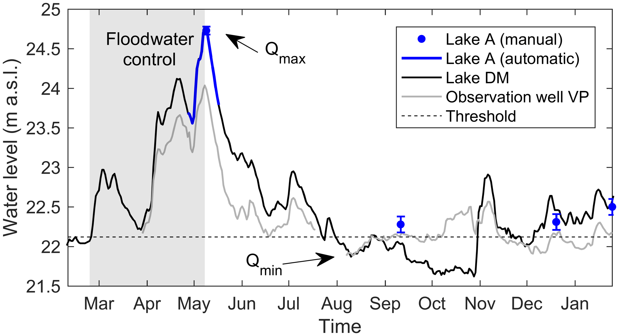
Figure 2Daily mean water levels at lake A, lake DM, and observation well VP from 9 February 2017 to 25 January 2018. The grey shaded area corresponds to the floodwater control period. Qmax and Qmin indicate the timing of the adjusted maximum and minimum output from the lake.
The water level in lake A was equivalent to lake DM during the flood peak (on 8 May 2017) and daily mean water levels at lake A and lake DM show good correlation (R2=0.98 and p value < 0.01) for the observed period (27 April to 17 May 2017). Daily mean water levels at observation well VP and lake DM also follow a similar pattern from late February to late July 2017 (R2=0.93 and p value < 0.01). Considering the above and a visible hydraulic connection between the lake DM and lake A, the data indicate that the daily water level variations at observation well VP were controlled by lake DM from late February to late July 2017. The lake A water level was also presumably controlled by lake DM until late July 2017, but technical issues prevented confirmation (i.e. the logger in lake A broke on 17 May 2017).
Then, from August to late October 2017, the water level in lake DM was below the topographical threshold, and there is no similarity between the evolution of the water level at lake DM and observation well VP (R2=0.11 and p value > 0.01). It is, thus, possible to infer that the lake A water level was not controlled by lake DM from August to late October 2017. This is also supported by the manual measurement of the lake A water level in September.
The water level of lake DM exceeded the topographic threshold again from November 2017 to January 2018, but the daily mean water levels at lake DM and observation well VP show a moderate correlation (R2=0.63 and p value < 0.01). The manual measurements also indicate a discrepancy between lake DM and lake A water levels in December 2017 and January 2018. The weaker correlation between the water level measurements suggests that lake DM was not controlling the dynamics of the lake A water level. It is, thus, likely that lake A received little to no surface water inputs from lake DM from November 2017 to January 2018. In this context, surface water inflows from lake DM during autumn and winter are considered negligible in this study and not included in the developed stable isotope mass balance model (Sect. 4.2).
2.3 Conceptual model of lake A water balance
Based on the geological and hydrological setting of the study site (Sect. 2.1) and flood-specific considerations (Sect. 2.2), we established a conceptual model of the lake A water balance, as described below.
Considering that lake A is sitting in alluvial sands (i.e. a highly permeable material), it is assumed that groundwater inputs (IG) and outputs (QG) contribute to the water budget. Although it is difficult to interpret the location of IG, it appears evident that QG occur along the NE bank of lake A. In fact, there are subsurface fluxes across the sandy bank that contribute to the bank filtration system or discharge into lake B, as its water level has been lower since the initiation of the bank filtration system (Masse-Dufresne et al., 2019). Given the regional groundwater flow in the NE to SW, QG can also presumably occur along the SW bank of lake A. Besides, it is likely that little to no subsurface fluxes exist in the area between lake A and lake DM, where clayey sediments are found.
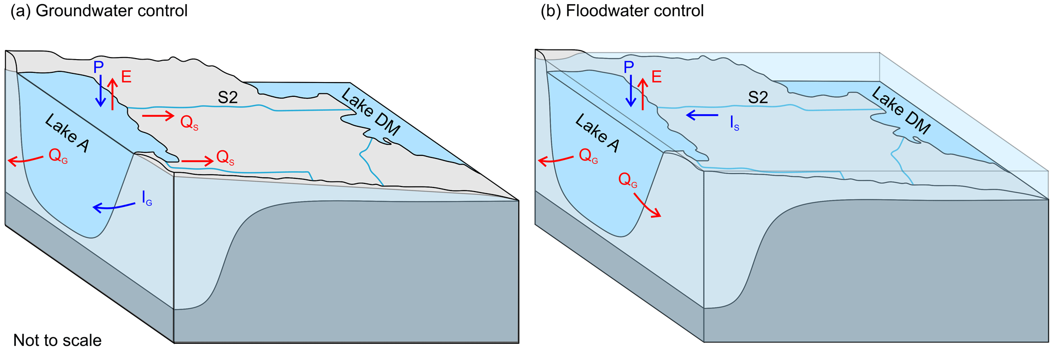
Figure 3Schematic representation of the hydrological processes at lake A during (a) groundwater control and (b) floodwater control periods. Inputs include precipitation (P), surface water (IS), and groundwater (IG), while outputs include evaporation (E), surface water outflow (QS), and groundwater outflow (QG). The area between lake DM and lake A is flooded in (b), and IS from lake DM contribute to the water balance of lake A.
For the study period, it is conceptualized that the direction of the surface water fluxes in S2 and S3 is from lake A to lake DM, except from 27 February to 8 May 2017. During this period (hereafter referred to as the floodwater control period), the water level of lake DM exceeds the topographic threshold, and lake A receives surface water inflow (IS) from lake DM. Also, it is likely that the high water level in lake A imposed a hydraulic gradient at the lake–aquifer interface, which allowed for QG from the lake and inhibited IG. Then, as lake A and lake DM water levels started to decrease (from 8 May 2017), it is assumed that water exits lake A as surface water outputs (QS) towards lake DM or as QG. Although lake DM's water level again exceeded the topographic threshold from November 2017 to January 2018, the weaker correlation between the water levels suggests that the lake A water level was not controlled by lake DM. In this context, we conceptualized that lake A water level variations are mainly controlled by groundwater flows (IG and QG). Surface water inputs (IS) are set to zero during this period (see Sect. 2.2).
To summarize, for the year 2017, the lake A water budget can be conceptualized with two distinct hydrological periods, i.e. (a) the groundwater control period and (b) the floodwater control period (Fig. 3). While the groundwater control period concerns most of the hydrological year, the floodwater control period only applies from 23 February to 8 May 2017. During the groundwater control period (Fig. 3a), it is assumed that groundwater inflows (IG) and precipitation (P) constitute the total water inputs to lake A, while surface water inflows (IS) are negligible. During this period, the outputs are occurring through evaporative fluxes (E), surface water outflows (QS), and groundwater outflows (QG). In contrast, it is assumed that IS and P represent the total water inputs to lake A during the floodwater control period (Fig. 3b). High water levels at lake A impose a hydraulic gradient at the lake–aquifer interface, which allows for QG and inhibits IG.
3.1 Field measurements
Pressure–temperature loggers (Diver®; TD-Diver and CTD-Diver; Van Essen Instruments B.V., Delft, the Netherlands) were used to measure surface water levels at lake A and groundwater levels at observation well VP on a 15 min time step. Water levels were recorded from 27 April 2017 (after the ice cover melted) to 17 May 2017 at lake A and from 29 March 2017 to 25 January 2018 (except between 19 July and 6 August 2017) at observation well VP. All the level loggers' clocks were synchronized with the computer's clock when launching automatic measurements. This procedure was done via the Diver-Office 2018.2 software. Manual measurements of the water level were regularly performed to calibrate (relative to a reference datum) and validate the automatic water level measurements. A level logger was also used to measure on-site atmospheric pressure and perform barometric compensation on water level measurements. Also note that water levels in lake A were not continuously recorded after 17 May 2017 due to a logger failure, but manual water level measurements (in September 2017, December 2017, and January 2018) depict the general evolution of lake A's water level.
Mean daily water levels at lake DM were retrieved with permission from the Centre d'expertise hydrique du Quebec database (Centre d'expertise hydrique du Québec, 2020). Meteorological data were measured at land-based meteorological stations near the study site and obtained from the Environment and Climate Change Canada database (available online at https://www.weatherstats.ca/, last access: 30 September 2019). Daily air temperature, relative humidity, wind speed, dew point, and atmospheric pressure were measured at the Montréal–Mirabel International Airport station (45.68∘ N, −74.04∘ E; 18 km from the study site). Daily precipitation and solar radiation were measured at Sainte-Anne-de-Bellevue station (45.43∘ N, −73.93∘ E; 10 km from the study site) and Montréal–Trudeau International Airport station (45.47∘ N, −73.75∘ E; 17 km from the study site), respectively.
3.2 Water sampling and analytical techniques
Physico-chemical parameter measurements and water sampling were performed at lake A at approximately 0.3 m below the surface and 1 m from the lake shoreline (at LA-S1) on a weekly to monthly basis from 9 February 2017 to 25 January 2018. Physico-chemical parameters (including temperature, electrical conductivity, pH, and redox potential) were measured using a multiparameter probe (YSI Pro Plus 6051030 and Pro Series pH/ORP/ISE and Conductivity Field Cable 6051030-1; YSI Incorporated, Yellow Springs, OH, USA). Additionally, vertical profile measurements and depth-resolved water sampling were conducted on 9 February 2017, 17 August 2017, and 25 January 2018 (at LA-P1 to LA-P4). Lake A water sampling was performed in the northern part of the lake for logistical reasons and due to ease of accessibility. As horizontal homogeneity has been previously demonstrated by Pazouki et al. (2016), the water samples were deemed representative of the whole waterbody.
Floodwater was sampled at two locations (near S2 and S3) on 19 April 2017 and at lake DM on 10 May 2017. Water samples were also collected at the surface and at depth within lake B and at observation well Z16, which is upstream of lake B and, thus, representative of the regional groundwater contributing to the latter (Ageos, 2016).
Water samples were analysed for major ions, alkalinity, and stable isotopic compositions of water (δ18O and δ2H). Water was filtered in the field using 0.45 µm hydrophilic polyvinylidene fluoride (PVDF) membranes (Millex-HV; Millipore, Burlington, MA, USA) prior to sampling for major ions and alkalinity. From December to March, cold weather prevented field filtration, so this procedure was performed in the laboratory on the same day. All samples were collected in 50 mL polypropylene containers and cooled during transport to the laboratory. The samples were then kept refrigerated at 4 ∘C until analysis, except for stable isotopes, which were stored at room temperature. Major ions were analysed within 48 h via ionic chromatography (ICS 5000 AS-DP Dionex; Thermo Fisher Scientific, Saint-Laurent, QC, Canada) at Polytechnique Montréal (Montreal, Quebec). The limit of detection was ≤0.2 mg L−1 for all major ions. Bicarbonate concentrations were derived from alkalinity, which was measured manually in the laboratory according to the Gran method (Gran, 1952) at Polytechnique Montréal (Montreal, Quebec). On samples with measured alkalinity (n=12), the ionic balance errors were all below 8 %. The mean and median ionic balance errors were 1 %. Stable isotopes of oxygen and hydrogen were measured with a water isotope analyser with off-axis integrated cavity output spectroscopy (LGR-T-LWIA-45-EP; Los Gatos Research, San Jose, CA, USA) at Geotop-UQAM (Montreal, Quebec). In total, 1 mL of water was pipetted in a 2 mL vial and closed with a septum cap. Each sample was injected (1 µL) and measured 10 times. The first two injections of each sample were rejected to limit memory effects. A total of three internal reference waters ( ‰, ‰ and ‰; ‰, ‰, and ‰) were used to normalize the results on the Vienna Standard Mean Ocean Water–Standard Light Antarctic Precipitation (VSMOW–SLAP) scale. A fourth reference water ( ‰; ‰) was analysed as an unknown to assess the exactness of the normalization. The overall analytical uncertainty (1σ) is better than ±0.1 ‰ for δ18O and ±1.0 ‰ for δ2H. This uncertainty is based on the long-term measurement of the fourth reference water and does not include the homogeneity nor the representativity of the sample.
3.3 Stable isotope mass balance
Stable isotope mass balances for lakes can either be performed based on (i) a well-mixed single layer model or (ii) a depth resolved multi-layered model. Arnoux et al. (2017c) performed a comparison of both methods and reported that well-mixed and depth-resolved multi-layered models yielded similar results and showed that groundwater inputs and outputs play an important role in lake water budgets. Arnoux et al. (2017c) further highlighted that the multi-layer model additionally allowed for the determination of groundwater flow with depth but required a temporally and depth-resolved sampling in order to ensure a thorough understanding of the stability/mixing of the different layers. Such time-consuming sampling and monitoring efforts are, however, often unrealistic in remote and/or flood-affected contexts. Additionally, Gibson et al. (2017) showed that the timing of the lake water sampling may introduce greater bias in a well-mixed isotopic mass balance model than the uncertainty related to the lake stratification. For these reasons, we opted to develop a well-mixed model in the context of this study. Note that, despite the biases underlying well-mixed models, this approach remains adequate for characterizing the relative importance of hydrological processes and is particularly useful for giving first-order estimates of water fluxes in ungauged basins.
The water and stable isotope mass balance of a well-mixed lake can be described, respectively as Eqs. (1) and (2) as follows:
where V is the lake volume, t is time, I is the instantaneous inflow, E is evaporation, and Q is the instantaneous outflow. I corresponds to the sum of surface water inflow (IS), groundwater inflow (IG), and precipitation (P). Similarly, Q is the sum of surface water outflow (QS) and groundwater outflow (QG). δL, δI, δE, and δQ are the isotopic compositions of the lake, I, E, and Q, respectively. In the context of this study, the balance equations can be simplified based on the conceptual model. During the groundwater control period, IS=0 and, thus, and . In contrast, IG=0 during the floodwater control period, and . Note that δG and are the isotopic signatures of groundwater and surface water inputs, respectively.
The application of Eqs. (1) and (2) for both δ18O and δ2H is valid during the ice-free period and also assumes the constant density of water (Gibson, 2002). In this study, the potential impacts of the ice cover formation and melting are neglected, as the ice volume is likely to represent only a small fraction (<2 %) of the entire water body. Moreover, considering the ice water isotopic separation factor, i.e. 3.1 ‰ for δ18O and 19.3 ‰ for δ2H (O'Neil, 1968) and assuming well-mixed conditions, the lake water isotopic variation would be comprised within the analytical uncertainty. Also, floodwater inputs from lake DM were expected to be much more important and occurring simultaneously with ice melt during the freshet period.
Thus, a volume-dependent model is applied, as described in Gibson (2002). The change in the isotopic composition of the lake (δL) with f (i.e. the remaining fraction of lake water) can be expressed as Eq. (3) as follows:
where is the fraction of lake water lost by evaporation, is the fraction of lake water lost to liquid outflows, m is the temporal enrichment slope (see Appendix B), δ0 is the isotopic composition of the lake at the beginning of the time step, and δS is the steady-state isotopic composition the lake would attain if f tends to 0 (see Appendix B).
A step-wise approach is used to solve Eq. (3) on a daily time step. At each time step, recalculation of is needed, where V is the residual volume at the end of the time step and V0 the original volume at the beginning of the time step (or Vt−dt). Hence, Eq. (3) is based on the water level difference between 2 d. The water flux parameters (E, I, and Q) and isotopic signatures (δE, δA, δI, and δQ) are thus evaluated on a daily time step.
The flushing time (tf) is defined as the ratio of the volume of water in a system to the rate of renewal (Monsen et al., 2002). In this study, tf by groundwater inputs is considered and is expressed as follows:
3.4 Daily volume changes at lake A and water fluxes
The initial lake volume (4.7×10⁶ m3) was estimated from the observed lake surface area (2.79×10⁵ m2) and the maximal depth (20 m) and assuming bank slopes of 25∘. Assuming bank slopes of 20 or 30∘, a typical range for saturated sands (Holtz and Kovacs, 1981), would result in an estimated initial lake volume of 4.84×10⁶ m3 (+3 %) and 4.32×10⁶ m3 (−8 %). Lake A volume variations are estimated from daily water level changes and assuming a constant lake area. As water level measurements are only available for a short period at lake A, water levels at lake DM and observation well VP are used as proxies. Water levels at observation well VP were used as a proxy from 24 August to 30 October 2017, while water levels at lake DM were assumed representative of lake A for the rest of the study period (i.e. from 9 February to 23 August 2017 and from 31 October 2017 to 25 January 2018). This approximation is deemed acceptable because the simulation of δL depends on the remaining fraction of lake water f (not the absolute water level), and daily variations in the water levels at lake A, lake DM, and observation well VP were shown to be similar (see Sect. 2.2).
Evaporative fluxes (E) are calculated using the standardized Penman-48 evaporation equation, as described in Valiantzas (2006), as follows:
where Rn is the net solar radiation (megajoules per square metre per day), Δ is the slope of the saturation vapour pressure curve (kilopascals per degree Celsius; hereafter kPa ∘C−1), γ is the psychrometric coefficient (kPa ∘C−1), λ is the latent heat of vaporization (megajoules per kilogram), f(u) is the wind function (see Appendix B), and D is the vapour pressure deficit. For comparative purposes, estimation of the daily evaporative fluxes was also conducted with the Linacre-OW equation (Linacre, 1977) and the simplified Penman-48 equation (Valiantzas, 2006). These methods yielded similar evaporation estimates from April to August but underestimated total evaporation by 24 % to 33 % compared to the standardized Penman-48 equation. The discrepancy between the models is restricted to late summer and autumn (see Appendix C; Fig. C1) and is attributed to the difference between the air and water surface temperature, which was estimated based on the equilibrium method as described by de Bruin (1982; see Appendix D). Note that E and P are set to zero during the ice cover period (i.e. from 1 January to 31 March, based on meteorological data and field observations).
For well-mixed conditions, the and are assumed to be equal to δL. Hence, no separation of these two fluxes is attempted, and they are merged into one variable, i.e. the outflow (Q). The direction and intensity of the water flux at the lake–aquifer interface can be conceptually described by Darcy's law, which states that Q=KAi, where K is the hydraulic conductivity, A is the cross-sectional area through which the water flows, and i is the hydraulic gradient. Given the significant depth of lake A (i.e. 20 m) in comparison to the maximum water level change during the flooding event (i.e. 2.7 m), the variations in A and K are expected to have a minor impact on Q. Hence, the change in outflows from the lake is expected to be mainly controlled by i changes and, consequently, to be roughly proportional to the change in lake water level. Considering the above, it was assumed that the daily outflow flux from lake A varied linearly according to the lake water level; the minimum and maximum outflow (Qmin and Qmax) correspond to the minimum and maximum water level, respectively. The outflow range (i.e. minimum and maximum values) was adjusted to obtain the best fit between the calculated and observed δL.
Total daily inflow (sum of daily P, IS, and IG) into lake A compensates for the adjusted daily outflow and daily lake volume difference. The precipitation (P) is evaluated from the available meteorological data (see Sect. 3.1), while direct measurement of IS and IG was not possible in this hydrogeological context (see Sect. 2.1). Consequently, further assumptions are needed to apportion these contributions. Considering the proposed conceptual model of the groundwater–surface water interactions (see Sect. 2.2), IS is set to zero, while IG is contributing to the lake during the groundwater control period. On the other hand, during the floodwater control period (i.e. from 23 February to 8 May 2017), it is assumed that the rising water level at lake A results in a hydraulic gradient forcing the lake water to infiltrate into the aquifer, inhibiting IG.
From 23 February to 8 May 2017, the net water fluxes are mainly positive, and an overall volume increase is observed at lake A. The maximum volume change of lake A was 7.6×10⁵ m3, which represents 16 % of the lake's initial volume. The maximum net water flux was 1.2×10⁵ m3 d−1, corresponding to a water level rise of 0.43 m (on 5 April 2017 only). From 9 May to mid-August 2017, lake A volume was decreasing, and the daily net water fluxes were mainly negative. In early August 2017, lake A regained its initial volume. Then, in autumn and winter, the volume of lake A was oscillating, and the net water fluxes were ranging from to 5.3×10⁴ m3 d−1. At the end of the study period (i.e. on 25 January 2018), a net volume difference of 1.5×10⁵ m3 remained at lake A compared to 9 February 2017.
However, the evolution of lake A volume and the net water fluxes are not representative of the surface water–groundwater interactions. Indeed, gross water fluxes are likely to exceed net water fluxes at natural and dredged lakes sitting in permeable sediments (Zimmermann, 1979; Arnoux et al., 2017a; Jones et al., 2016). In the context of this study, we conceptualized two main hydrological periods during which the lake water can either drain towards lake DM or exit the lake as groundwater output. To balance out these outputs, the inflows to lake A must therefore be greater than the net water fluxes.
For that reason, the development of a volume-dependent transient stable isotope mass balance was required to correctly depict the importance of the floodwater inputs on the water mass balance of the lake.
4.1 Isotopic and geochemical framework
The isotopic composition of precipitation (δP), lake A, and floodwater are depicted in Fig. 4. The local meteoric water line (LMWL) was defined using an ordinary least squares regression (Hughes and Crawford, 2012) using isotope data in precipitation from the Saint-Bruno station RIGR (Research Infrastructure on Groundwater Recharge) database (n=27; from December 2015 to June 2017).
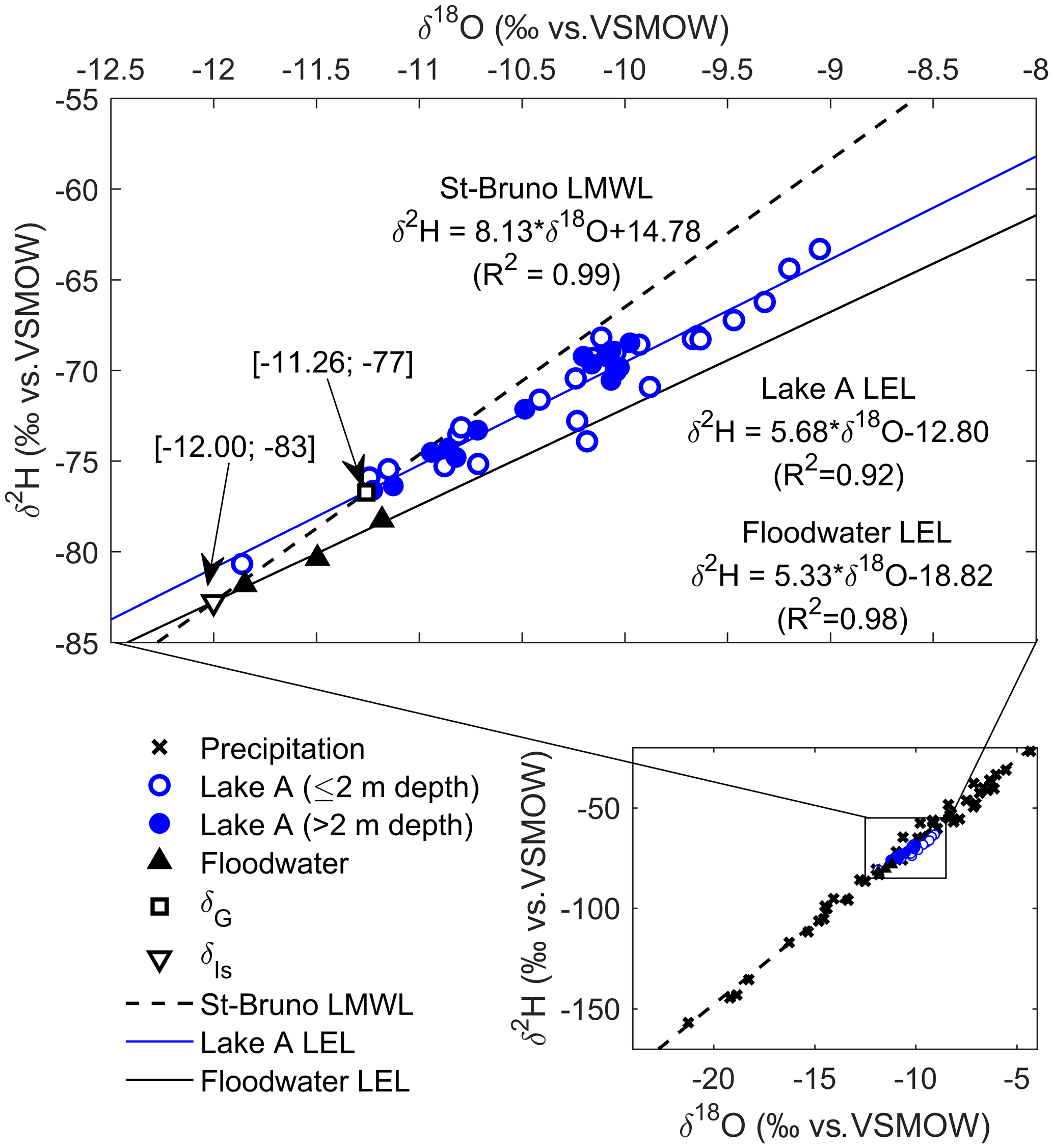
Figure 4Isotopic composition of precipitation, lake A water, and floodwater from March 2017 to January 2018. Hollow and solid blue circles correspond to samples collected at ≤2 and >2 m depth, respectively. Analytical precision is 0.15 ‰ and 1 ‰ at 1σ for δ18O and δ2H. Precipitation data are retrieved from the research infrastructure on groundwater recharge database (Barbecot et al., 2019).
For the study period, the isotopic composition of bulk precipitation was available on a biweekly to monthly time step (n=15) and ranged from −19.19 ‰ to −6.85 ‰ for δ18O and −144 ‰ to −38 ‰ for δ2H. Interpolation was used to simulate the δP on a daily time step for the isotope mass balance model computation.
Isotopic compositions of lake A water samples (n=39) are linearly correlated (see solid blue line) and all plotted below the LMWL, which confirms that lake A is influenced by evaporation. Linear regression of lake A water samples defines the local evaporation line (LEL), which is (R2=0.92). Some samples from the surface of lake A are plotted below the LEL, likely indicating snowmelt water inputs as noted in previous studies of Canadian lakes (Wolfe et al., 2007).
The isotopic composition of the floodwater samples (n=3) is indeed more depleted than lake A waters (i.e. δ18O from −11.85 ‰ to −11.18 ‰ and δ2H from −81 ‰ to −78 ‰) and is most likely reflecting the significant contribution from heavy isotope-depleted snowmelt waters. The floodwater samples are also linearly correlated and are plotted along a line () for which the slope is similar to lake A LEL, suggesting that the sampled floodwater evaporated under the same conditions as lake A water samples. For simplification purposes, the isotopic composition of the surface water inflow () was set to the intersection between the floodwater LEL and the LMWL ( ‰ and ‰). The long-term (1997–2008) average and minimum and maximum isotopic signatures of Ottawa River water at Carillon (∼34 km upstream from lake DM; see Fig. 1b) for the month of April are −11.19 ‰, −12.01 ‰ and −10.23 ‰ for δ18O and −81 ‰, −85 ‰ and −77 ‰ for δ2H, respectively (Rosa et al., 2016). The mean and minimum values compare well with the observed isotopic signatures at lake DM during springtime in 2017.
The isotopic composition of groundwater (δG) can be determined from direct groundwater samples or indirectly from the amount-weighted mean δP. However, in highly seasonal climates, there is a widespread cold season bias to groundwater recharge (Jasechko et al., 2017), and estimating δG via groundwater samples or an amount-weighted mean δP may be misleading. In fact, it has been argued that the LMWL–LEL intersection better represents the isotopic composition of the inflowing water to a lake and is, thus, commonly used to depict the δG in isotopic mass balance applications (Gibson et al., 1993; Wolfe et al., 2007; Edwards et al., 2004). Concerning the study site, the estimated δG is −11.26 ‰ for δ18O and −77 ‰ for δ2H (i.e. the Saint-Bruno LMWL and lake A LEL intersection). The latter compares well with the mean isotopic signature of groundwater at Saint-Télesphore station (−11.1 ‰ for δ18O and −78.5 ‰ for δ2H; Barbecot et al., 2018) and is more depleted than the long-term amount-weighted mean δP at Ottawa (−10.9 ‰ for δ18O and −75 ‰ for δ2H; IAEA/WMO, 2018). Note that the locations of Saint-Télesphore station and Ottawa are depicted in Fig. 1b.
The geochemical facies of lake A and lake DM samples are illustrated in Fig. 5 by the means of a Piper diagram. Mean values for lake B and regional groundwater (GW) geochemical facies are also plotted for comparison purposes. Both lake A and floodwater were found to be Ca-HCO3 types, which is typical for precipitation- and snowmelt-dominated waters (Clark, 2015). The geochemistry of lake A is relatively constant throughout the year and reveals a depth-wise homogeneity. The geochemistry of lake B is distinct from lake A and appears to be influenced by regional groundwater characterized by a Na-Cl water type.
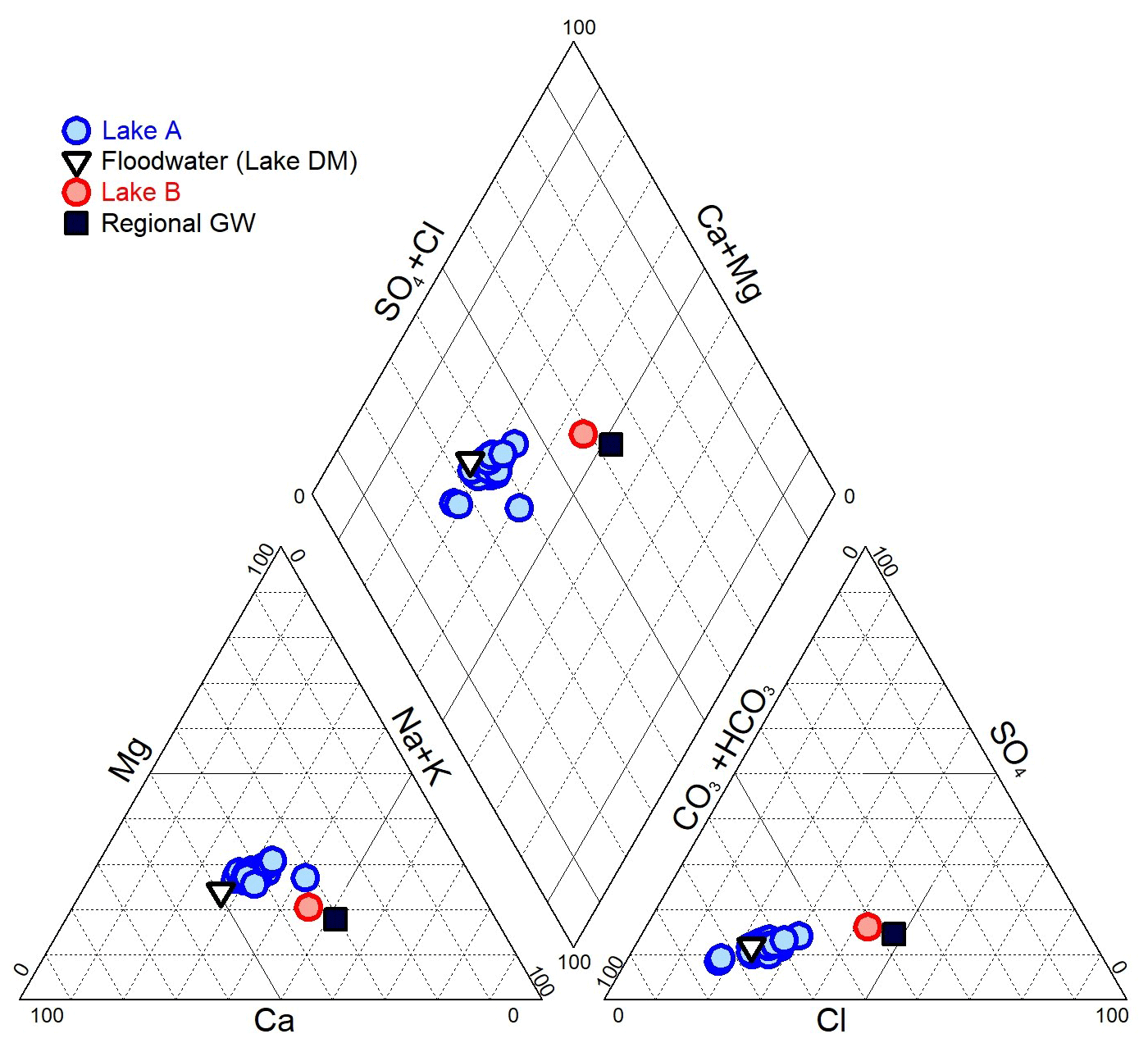
Figure 5Geochemical facies of lake A (n=23) and floodwater (n=1). Mean values for lake B (n=42) and regional groundwater (GW) (n=11) geochemical facies are also plotted. Lake A and floodwater are characterized by Ca-HCO3 water types, while lake B and regional GW correspond to Na-Cl water types. Note that regional GW was sampled upstream of lake B.
4.2 Evaluation of the water budget
4.2.1 Volume dependent isotopic mass balance model
As described in Sect. 3.3, the isotopic mass balance model was solved iteratively by recalculating δL on a daily time step. This model was developed assuming (1) well-mixed conditions and (2) that the outflow flux changes are roughly proportional to the lake's water level changes. We adjusted the minimum and maximum outflow fluxes (Qmin and Qmax) so that they corresponded to the minimum and maximum water levels (see Fig. 3).
In total, three sampling campaigns (i.e. on 9 February 2017, 17 August 2017, and 25 January 2018) were conducted at lake A in order to collect water samples for isotopic analyses from the epilimnion, metalimnion, and hypolimnion (Fig. 6; Appendix E; Fig. E1) to account for the vertical stratification of the isotopic signature (Gibson et al., 2017). The vertical isotopic profiles were volume-weighted according to the representative layer for each discrete measurement in order to obtain the observed δL for each campaign (Table 1). The depth-averaged isotopic composition of the lake on 9 February 2017 (i.e. ‰ and ‰) was used as the initial modelled δL.

Figure 6Observed and modelled depth-average isotopic composition of the lake (δL) for δ18O (a, b) and δ2H (c, d) from 9 February 2017 to 25 January 2018 for scenarios A and B. The hollow and solid blue circles correspond to lake A water samples collected at ≤2 and >2 m, respectively. The modelled δL is fitted against the three depth-averaged δL and an additional sample collected at ≤2 m depth on 9–10 May 2017 (scenario A) and 27 April 2017 (scenario B). These samples are marked by the hollow red squares. The grey shaded area corresponds to the floodwater control period. The error bars correspond to the standard error in the samples for each campaign. The dashed lines represent the modelled δL when considering that 25 % to 100 % of the outputs from the lake during the floodwater control period were temporally stored in the aquifer and discharged to the lake as floodwater-like inputs ().
Table 1Observed depth averaged (or mean) and standard deviation (SD) of isotopic composition of lake A for the sampling campaigns in February 2017, August 2017, and January 2018 and all samples. The isotopic composition of the samples collected at the surface of lake A on 9–10 May and 27 April 2017 are also listed. The asterisks (*) indicate that a mean value was calculated (instead of a depth-averaged value).
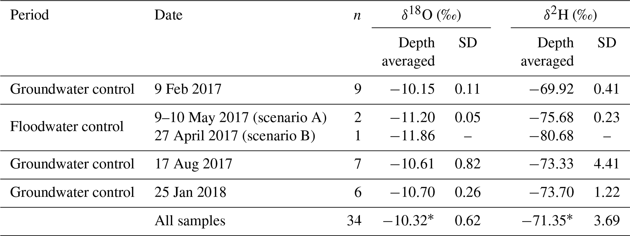
While depth-averaged δL was not available during the floodwater control period (i.e. late February to early May), water samples from the surface of lake A provide relevant evidence to better constrain the model. It is likely that lake A was fully mixed during the floodwater control period, and that the water samples collected at the surface of lake A on 27 April or 9–10 May 2017 are representative of the whole water body. Indeed, the observed surface water temperature was <5 ∘C until early May (see Fig. C1) and suggests a limited density gradient along the water column which does not allow for the development of thermal stratification. In this context, we opted to simulate two scenarios (A and B) for which the isotopic mass balance model is either constrained at ‰ and ‰ on 9–10 May 2017 or at ‰ and ‰ on 27 April 2017.
The results of the volume-dependent isotopic mass balance for δ18O and δ2H are illustrated in Fig. 6. The fitted Qmin and Qmax from lake A are 3.7×10⁴ and 8.0×10⁴ m3 d−1 for scenario A and 1.0×10³ and 2.8×10⁵ m3 d−1 for scenario B. These first-order water flux estimates represent equivalent water level variations ranging from 0.004 and 1.0 m d−1. From 23 February to 8 May 2017 (see the grey shaded area), hydraulic conditions allowed for surface inputs (IS) from lake DM to lake A at a mean rate of 6.61×10⁴ m3 d−1, with a total floodwater volume of 4.82×10⁶ m3 for scenario A. The total floodwater volume was twice as important (9.96×10⁶ m3) for scenario B. Then, from 9 May 2017, we considered that these floodwater inputs stopped as the lake water level started to decrease. As a consequence, the model yielded a gradual enrichment of δL due to the combined contribution from IG and E for both scenarios. From 9 May 2017 to 25 January 2018, the total IG were 1.16×10⁷ and 1.48×10⁷ m3 for scenario A and B, respectively. Overall, the δ18O and δ2H models were better at reproducing the January 2018 and August 2017 observed δL, respectively. This is likely linked to the uncertainties and representativeness of the meteorological data, which is controlling the isotopic fractionation due to evaporation.
While the computed flows for scenario A are within a plausible range for the combination of surface and groundwater outflow processes (i.e. minimum and maximum equivalent water level variations of 0.13 and 0.29 m d−1), scenario B yielded less realistic results (i.e. minimum and maximum equivalent water level variations of 0.004 and 1.0 m d−1). As mentioned above, scenario B was constrained at ‰ and ‰ in late April (Fig. 6), based on a surface water sample which was taken during a temporarily decreasing water level period (Fig. 3) and is, thus, likely less representative of the overall lake's dynamics compared to scenario A. This demonstrates the limit of the approach and shows that it is important to correctly constrain the model during flood events in order to perform precise estimations of the water balance.
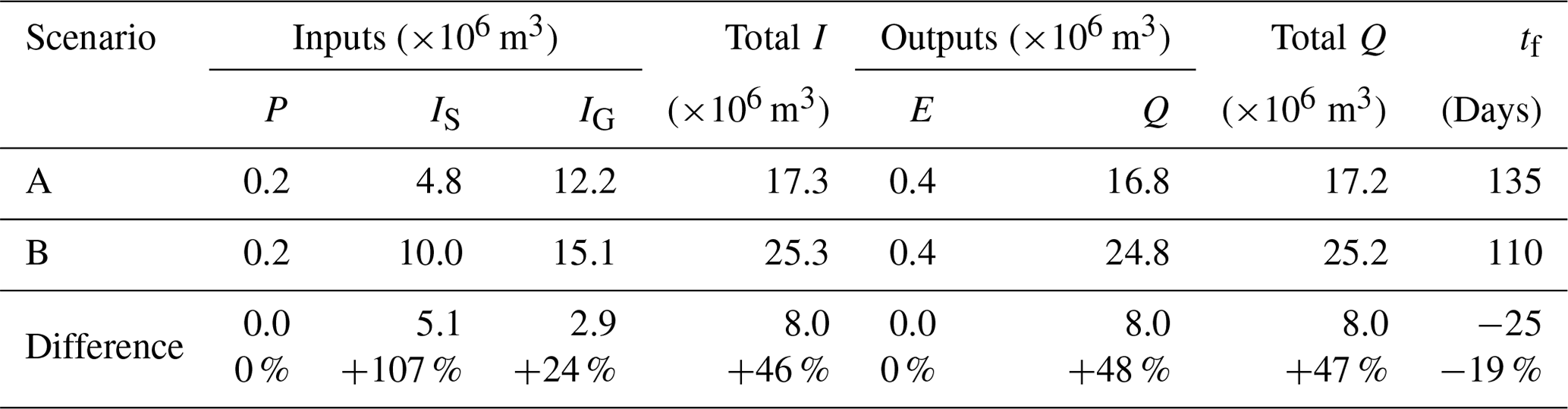
The water mass balance of lake A from 9 February 2017 to 23 January 2018 is summarized in Table 2 for both scenarios. The difference between the total inputs and total outputs correspond to the lake volume difference (1.48×10⁵ m3) between the start and the end of the model run. Groundwater inputs (IG) and surface water inputs (IS) account for 71 % and 28 % of the total water inputs to the lake for scenario A. While IS are twice as important for scenario B, they only account for 39 % (+11 %) of the total inputs, and the IG are 60 % (−11 %). It thus appears that the annual dynamic of lake A is dominated by groundwater inputs for both scenarios, despite the intensity of the flood event. For scenarios A and B, tf, as defined in Eq. (4), is similar (i.e. 135 and 110 d). Precipitation is contributing 1 % of the total annual inputs and evaporation only accounts for 2 % of the total annual outputs. Although the establishment of a hydraulic connection between lake DM and lake A is a recurring yearly hydrological process, it is important to note that the magnitude and duration of the flooding event of 2017 was particularly important and, thus, had a greater impact on the dynamic of lake A in comparison to other years.
Table 2Water mass balance of lake A for scenarios A and B. The difference between the total inputs and total outputs corresponds to the lake volume difference over the study period. The total inputs (I) correspond to the sum of precipitation (P), surface water inflow (IS), and groundwater inflow (IG). The total outputs (Q) correspond to the sum of evaporation (E) and surface water and groundwater outflow (Q). The mean flushing time (tf) is the ratio of the lake volume to the mean groundwater inputs (IG).
4.2.2 Sensitivity analysis
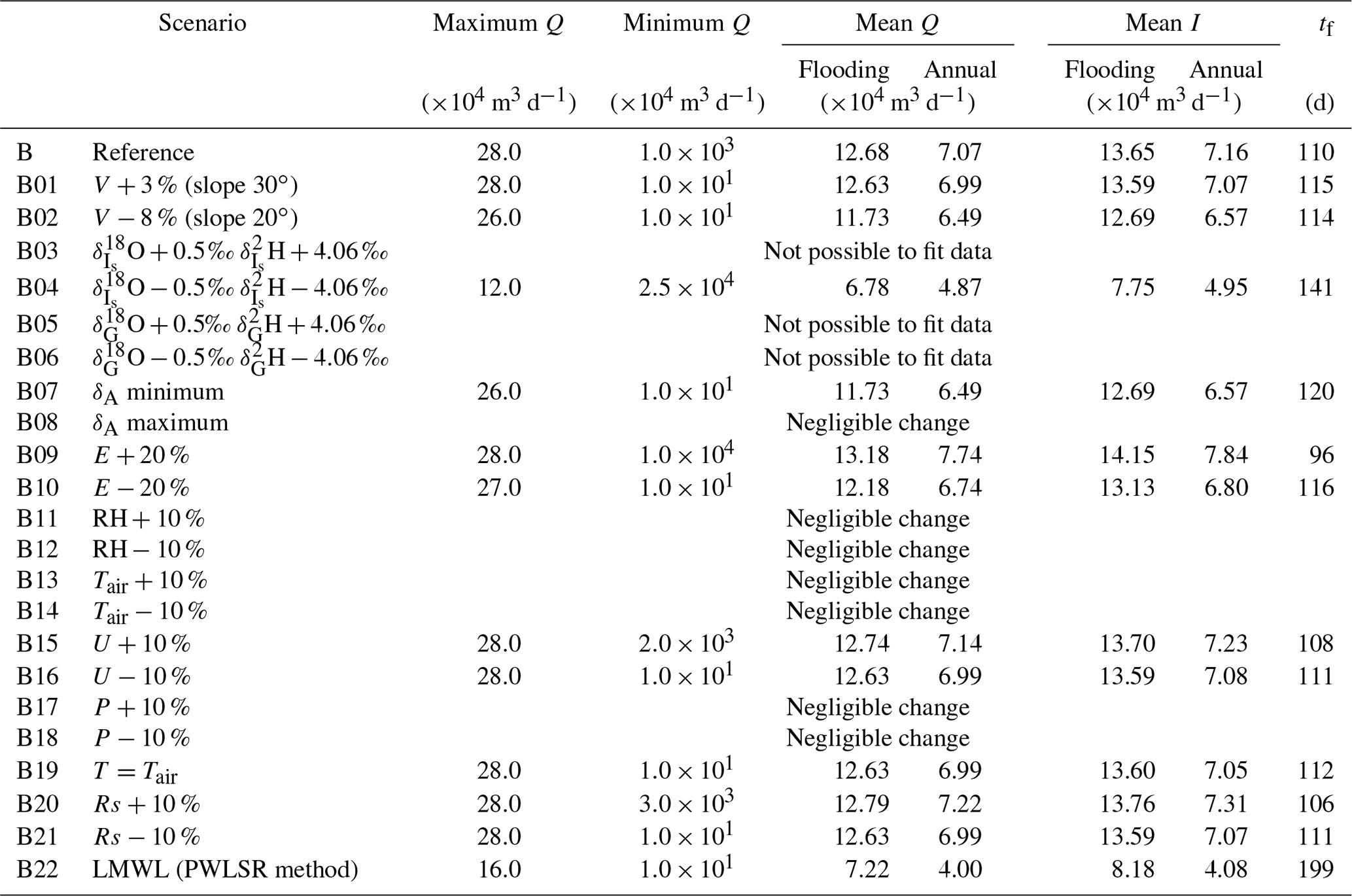
A one-at-a-time (OAT) sensitivity analysis was performed to grasp the relative impact of the input parameters' uncertainties on the model outputs. For each parameter, we tested two scenarios which delimit the uncertainty for each parameter. First, we tested the sensitivity of the model for V+3 % and V−8 % (i.e. estimated with slopes of 30 and 20∘). Concerning and δG, the model was tested for ±0.5 ‰ for δ18O and ±4 ‰ for δ2H, assuming they would both evolve along the LMWL (see Fig. 3). Then, we assessed the sensitivity of the model to δA by fixing the seasonality factor k at 0.5 and 0.9. Evaporation was computed with ±20 %, whereas the meteorological parameters (i.e. relative humidity (RH), Tair, U, P, and Rs) were tested for ±10 %. As E and δA are dependent on the water surface temperature, we also tested the sensitivity of the model when considering that T is equal to the daily mean air temperature (Tair). Finally, we tested for the uncertainties concerning the definition of the LMWL. For the reference scenario, the LMWL () was estimated using an ordinary least square regression (OLSR). For the sensitivity analysis, we estimated the LMWL via a precipitation amount weighted least square regression (PWLSR), which was developed by Hughes and Crawford (2012). Using the PWLSR method, the LMWL is defined as , and and δG are estimated at −12.39 ‰ and −11.74 ‰ for δ18O and at −85 ‰ and −79 ‰ for δ2H, respectively. Recalculation of and δG was needed, as they were both assumed to be plotted on the LMWL (see Sect. 4.1).
The results of this sensitivity analysis are listed in Tables F1 and F2 (Appendix F) for scenarios A and B. Overall, the model was found to be highly sensitive to the uncertainties associated with , δG, and E, as the annual mean water fluxes (Q and I) varied up to −31 % and +46 % compared to the reference scenarios A and B. A negligible to slight change in the modelled δL was found when considering the uncertainties for V, δA, RH, Tair, U, P, and Rs. For these variables, the mean flux estimate (Q and I) changes ranged from −8 % to +4 % compared to the reference scenarios A and B. As expected, the value of affects the modelled δL exclusively during the floodwater control period. Similarly, the values of δG and E particularly influence the modelled δL from late summer to early winter. This is due to the fact that Q and E are the dominant fluxes during this period. When considering that T is equal to Tair, despite the significantly different maximum and minimum values for Q, the mean Q was relatively similar to the reference scenarios, and only a small change for tf (+3 % and +2 % compared to reference scenarios A and B) was found. Finally, the model is highly sensitive to the uncertainties associated with the LMWL, as a translation of the LMWL implies an enrichment or depletion of both the , δG at the same time. Such modifications result in mean flux estimate (Q and I) changes of up to −38 % and −43 % compared to reference scenarios A and B.
4.3 Importance of temporary floodwater storage on the water balance partition
The developed isotopic mass balance model yielded significant floodwater inputs during springtime to be a best fit to the observed δL. A first-order estimate of the total floodwater volume summed to 4.82×10⁶ m3 (for scenario A), which is nearly equal to the lake's initial volume (i.e. 4.70×10⁶ m3). Similar results were obtained by Falcone (2007), who studied the hydrological processes influencing the water balance of lakes in the Peace–Athabasca Delta, Alberta (Canada) using water isotope tracers. They reported that a springtime freshet (in 2003) did replenish the flooded lakes from 68 % to >100 % (88 % on average).
As mentioned in Sect. 2.3, it was conceptualized that the high surface water elevation of lake A during springtime resulted in hydraulic gradients that forced lake water to infiltrate into the aquifer and induce local recharge (see Fig. 3). An important volume of flood-derived water could, thus, be stored during the increasing water level period and eventually discharged back to the lake as its water level decreased. Hence, the groundwater inputs to lake A following the flooding event likely corresponded to flood-derived surface water originating from lake DM. Considering that these fluxes are characterized by a floodwater-like isotopic signature (), rather than the isotopic signature of groundwater (δG), the temporal evolution of the modelled δL would be modified. Such a consideration is noteworthy for a better depiction of the importance of floodwater inputs in the water balance partition.
Assuming that 25 % to 100 % of the outputs (Q) from the lake during the floodwater control period were temporally stored in the aquifer and did eventually discharge back to the lake, the modelled δL diverges more or less from the reference scenarios A and B (Fig. 6; see the dashed lines). It is noteworthy that a better fit between the modelled δLand depth-averaged δL is obtained when considering that 25 % to 50 % of the outputs (Q) from the lake during the floodwater control period discharge back to the lake. In fact, it is likely that part of the potential stored floodwater could have effectively discharged back to the lake. For instance, part of the floodwater-like groundwater could have been abstracted by the pumping wells at the adjacent bank filtration site or could have been discharged to lake B. These results illustrate the importance of considering temporary subsurface floodwater storage when assessing water balances, especially as the magnitude and frequency of floods are likely to be more important in the future (Aissia et al., 2012).
4.4 Temporal variability in the water balance partition
The water balance presented in Table 2 provides an overview of the relative importance of the hydrological processes at lake A for the study period (i.e. February 2017 to January 2018). As the surface water inputs (as floodwater) only occurred during springtime at lake A, it is also important to decipher the temporal variability in the water fluxes. The dependence of a lake on groundwater can be quantified via the G index, which is the ratio of cumulative groundwater inputs to the cumulative total inputs (Isokangas et al., 2015). Figure 7 shows the temporal evolution of the G index from 9 February 2017 to 25 January 2018 for scenario A and the associated scenarios (A1 to A22) considered in the sensitivity analysis. Note that the G index is calculated at a daily time step, based on the cumulative water fluxes. It is used to understand the relative importance of groundwater inputs over the studied period and does not consider the initial state of the lake. In early February, the G index was 100 % because no surface water inputs (IS) or precipitation (P) had yet contributed to the water balance. During the floodwater control period (see grey shaded area), the G index rapidly decreased and reached 12 % on 8 May 2017 (for the reference scenario A). A gradual increase in the G index is then computed for the rest of the study period. On 25 January 2018, the G index is 71 % and is likely more representative of annual conditions. Despite the sensitivity of the model to the input parameters, all scenarios yielded similar results. The G index ranged from 62 % to 75 % on an annual timescale for the different scenarios.

Figure 7Temporal evolution of the G index from 9 February 2017 to 25 January 2018 for scenario A and the associated scenarios considered in the sensitivity analysis (i.e. A1 to A22). The grey shaded area corresponds to the floodwater control period. The dashed lines correspond to the G index when considering that 25 % to 100 % of the outputs from the lake during the floodwater control period were temporally stored in the aquifer and discharged to the lake as floodwater-like inputs (IS, ).
The impact of the potential temporary subsurface storage is also depicted in Fig. 7 (see dashed lines). As highlighted in Sect. 4.3, part of the potentially stored floodwater in the aquifer could have discharged back to the lake as floodwater-like inputs () after the flooding event. Considering these fluxes as surface water inputs (IS), rather than groundwater inputs (IG), would alter the temporal evolution of the G index. Assuming that 25 % to 100 % of the outputs from the lake during the floodwater control period did eventually discharge back to the lake, the floodwater inputs would contribute to the lake water balance until early June to early August (Fig. 7). Lake A would, thus, be dependent on flood-derived water during a 1- to 3-month period after the flooding event. On an annual timescale, the temporary subsurface storage could lower the G index to a minimum value of 47 %.
5.1 Resilience of lakes to groundwater pollution
The resilience of a system has been defined as its capacity to cope with perturbations (i.e. internal and/or external changes) while maintaining its state (Cumming et al., 2005). In the case of a lake, perturbations can manifest as a change in the water quantity and quality contributing to the water balance. According to Arnoux et al. (2017b), the impact of a perturbation to a lake is not only dependent on the relative importance of water budget fluxes but also on the residence time of water in the lake. Thus, they proposed an interpretation framework which relates the response time of a lake to changes in groundwater quantity and/or quality, thereby linking the G index with tf, which is the mean flushing time by groundwater fluxes (Fig. 8). They depict a general case, applicable to any pollution, regardless of reactivity or the fate of contaminants. Hence, care should be taken when interpreting the sensitivity to specific contaminants which are subject to attenuation processes, such as degradation and sorption.
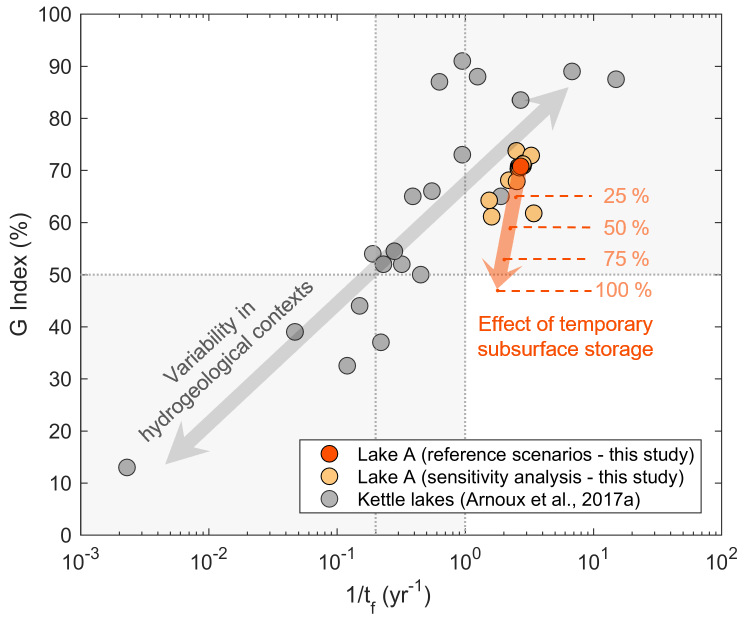
Figure 8Resilience of lakes to groundwater quantity and quality changes for lake A (this study) and kettle lakes (Arnoux et al., 2017b) in southern Quebec (Canada). The G index is the ratio of groundwater inputs to total inputs, and tf is the mean flushing time by groundwater. This representation is adapted from Arnoux et al. (2017b).
In their study, Arnoux et al. (2017b) assessed the resilience of kettle lakes (n=20), located in southern Quebec (Canada), in similar morpho-climatic contexts to lake A. The surveyed lakes were found to be characterized by a wide range of conditions, from resilient (i.e. G index < 50 % and tf>5 year) to highly sensitive to groundwater changes (i.e. G index > 50 % and tf<1 year). This is related to the variability in the hydrogeological contexts, resulting in variations in the importance of groundwater contributions and the range of mean flushing times of the lakes (see the grey arrow in Fig. 8). The majority of the lakes (i.e. 50 %) were found to be characterized by intermediate conditions (G index > 50 % and year) and, thus, were classified as being relatively resilient to both surface and groundwater changes.
Concerning lake A, studied scenarios (i.e. reference scenario A and the sensitivity analysis) yielded values for G index > 50 % and tf<1 year, i.e. indicating that lake A is highly sensitive to groundwater changes but resilient to surface pollution. Nevertheless, it was shown that temporary floodwater storage and discharge to lakes are crucial to correctly represent the G index by accounting for the origin of water fluxes (Fig. 7; Sect. 4.4). While floodwater storage lowers the G index, the tf slightly increases (see orange arrow in Fig. 8). Therefore, the studied lake receives a reduced groundwater contribution relative to the initial estimated apportionment when not accounting for floodwater storage but is still characterized by a rapid flushing time. This implies that flood-affected lakes are more likely to be characterized by an intermediate condition and, thus, are relatively resilient to groundwater quantity and quality changes. The geochemical data (Sect. 4.2) are in agreement with this interpretation. Indeed, a low mineralization and Ca-HCO3 water type at lake A is consistent with the significant floodwater contributions (to the lake and aquifer). In comparison, the neighbouring lake (i.e. lake B) does not undergo yearly recurrent flooding and was shown to be more mineralized with a Na-Cl water type, likely originating from the road salt contamination of regional groundwater (Pazouki et al., 2016). Biehler et al. (2020) similarly reported hydrological controls on the geochemistry of a shallow aquifer in an hyporheic zone, where the river stage influenced the mixing ratio between river water and the deeper aquifer.
Considering the above, it is possible to speculate about the potential future impacts of climate change on lake A. Globally, future meteorological scenarios are predicting changes in precipitation and climate extremes, including floods and droughts (Salinger, 2005). In Quebec (Canada), river stages are expected to increase across various watersheds in response to future climate scenarios (Roy et al., 2001; Dibike and Coulibaly, 2005; Minville et al., 2008). These hydrological responses could result in floods of longer duration and higher intensity (Aissia et al., 2012) and more pronounced droughts (Wheaton et al., 2007). Such changes could directly affect the quality of lake A. If flooding becomes more prevalent, enhanced floodwater input to lake A would likely occur. In this case, the surface water inputs from floods would buffer the sensitivity of lake A to groundwater quality changes originating from its watershed. On the other hand, if floods become less important and/or less frequent, we can expect that the water quality of lake A would be more dependent on regional groundwater quality. In such a case, the geochemistry of lake A could potentially shift towards that of lake B, and an increase in the salinity and the concentration of Na+, Ca2+, , and Cl− would be expected for lake A.
5.2 Implications for water management
Water budget assessments at natural lakes can serve as a tool for quantifying local human impacts (i.e. land use changes and climate changes) on water resources (Arnoux et al., 2017b). Based on the results of this study, it becomes apparent that water budget assessments at artificial lakes (such as lake A) can also be used to track human impacts on water resources. Recurring water budget assessments at a specific lake over time will serve to document changes in groundwater and surface water apportionment and can help to detect changes in local groundwater availability, and to anticipate impacts on local water supply utilities. As the response time of a lake to changes is controlled by its flushing time, the evolution of the G index will manifest at various rates. Indeed, lakes with different tf would reflect changes at different timescales. For instance, lakes with tf>5 year would be expected to respond to decadal changes, while lakes with tf<5 year would track annual or interannual variability. By analogy, we might postulate that it would be informative to study lakes with rapid response times (i.e. tf<1 year), as they will act as precursors of the evolution of nearby surface water bodies characterized by longer flushing times.
As demonstrated, isotopic approaches may be efficiently employed to solve water budget unknowns as the method can be performed at low cost and requires limited sampling and monitoring efforts for flood-affected environments which may be difficult or dangerous to monitor using traditional approaches. To enhance the effectiveness of our approach, the sampling strategy may be improved. First, surface water sampling for isotopic analyses is recommended during turnover periods (i.e. springtime and autumn) and should be combined with depth-resolved measurements of physico-chemical parameters to confirm the vertical homogeneity or stratification. Second, for long-duration flood events, monitoring of potential evolution in floodwater isotopic signatures could help to improve the accuracy and realism of the model. Groundwater-level monitoring and groundwater sampling in the vicinity of the lake could also help to strengthen the conceptual model by providing data to interpret the direction of groundwater fluxes and the variability in isotopic composition through time.
In this study, a volume-dependent transient isotopic mass balance model was developed and applied to a flood-affected lake in an ungauged basin in southern Quebec (Canada). This allowed for a better understanding of the resilience of a flood-affected lake to changes in the surface–groundwater water balance partition, for an understanding of the role of floodwater, and for predicting the resilience to groundwater quantity and quality changes for a local water supply. Given the contrasting isotopic signature of the floodwater, the isotopic mass balance model was effectively applied at the study site. We anticipate that the isotopic framework is likely to be transferable to other lake systems subject to periodic flooding, including lowland lakes fed by mountain floodwaters, river deltas, wadis, or nival (snowmelt-dominated) regimes, the latter of which dominates the high-latitude and high-altitude cold regions, including much of the Canadian landmass.
The isotopic mass balance model revealed that groundwater inputs dominated the annual water budget. To test the sensitivity, representativeness, and resilience of the model, several model scenarios were evaluated to account for uncertainty in important input variables. Despite sensitivity to some variables, all model scenarios considered in the sensitivity analysis converged on the results that lake A is mainly dependent on groundwater inputs and has a rapid (<1 year) flushing time by groundwater, suggesting that lake A would be highly sensitive to groundwater quantity and quality changes.
When taking into account potential subsurface storage, a better fit could be obtained between the modelled and depth-averaged isotopic signature of the lake, suggesting that the contribution of floodwater-like subsurface inputs is important to consider when assessing for water balance at flood-affected lakes. In fact, the increased contribution of surface water (from subsurface storage) resulted in a lower contribution from groundwater and, consequently, in an increased resilience to groundwater changes. This finding provides a basis for postulating the impact of climate change on the water quality of lake A. If the importance of floods increases, more floodwater inputs to lake A can be expected during springtime, causing increased recharge. In this case, the surface water inputs from floods would increase the resilience of flood-affected lakes to groundwater quantity and quality changes at the watershed scale. On the other hand, if floods become less severe and/or less frequent, we can expect that the water quality of flood-affected lakes becomes more dependent on regional groundwater quality. From a global perspective, performing water balance assessments at lakes with rapid flushing time (<1 year) can help to predict the evolution of other surface water bodies with longer flushing times in their vicinity and, therefore, is useful for establishing regional-scale management strategies for maintaining lake water quality.
Table A1Detailed source information and download links for the openly available geospatial data in Fig. 1. All data are openly available and are used in accordance with the Open Government Licence – Canada or the Open Data Policy, M-13-13, of the United States Census Bureau.
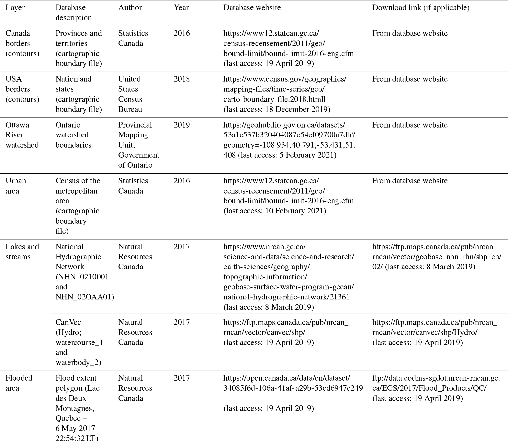
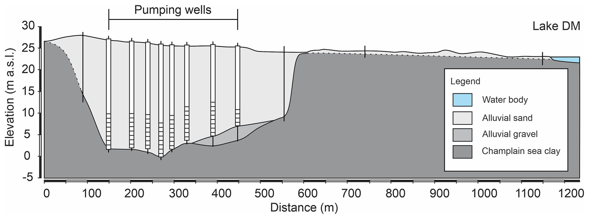
Figure A1Geological cross section along the pumping wells showing the buried valley carved into the Champlain Sea clays and filled with alluvial gravels and sands.
Computation of isotope mass balance parameters
The parameter f(u), for the estimation of E (Eq. 5), is calculated according to the area-dependent expression described by McJannet et al. (2012) as follows:
where u is the wind speed (metres per second) measured at 2 m above the ground, and A is the area (square metres) of the lake. Note that Eq. (6) was developed for land-based meteorological data.
The isotopic composition of the evaporating moisture (δE) is estimated based on the Craig and Gordon (1965) model and, as described by Gonfiantini (1986), is as follows:
where h is the relative humidity normalized to water surface temperature (in decimal fraction), δA is the isotopic composition of atmospheric moisture (described later on), ε+ is the equilibrium isotopic separation, and εK is the kinetic isotopic separation, with and (1 h). α+ is the equilibrium isotopic fractionation, θ is a transport resistance parameter, and CK is the ratio of molecular diffusivities of the heavy and light molecules. θ is expected to be close to 1 for small lakes (Gibson et al., 2015), and CK is typically fixed at 14.2 ‰ and 12.5 ‰ for δ18O and δ2H, respectively, in lake studies as these values represent fully turbulent wind conditions (Horita et al., 2008). Experimental values for α+ were used (Horita and Wesolowski, 1994) as follows:
where T is the water surface temperature (degrees Celsius), which was estimated according to the equilibrium method as described by de Bruin (1982) (see Appendix D).
The parameters m and δs, for the computation of δL (Eq. 3), are calculated as follows (Gibson, 2002):
where δ* is the limiting isotopic composition that the lake would approach as V→0 and is calculated as follows:
The isotopic composition of atmospheric moisture (δA) is estimated using the partial equilibrium model of Gibson et al. (2015) as follows:
where δP is the isotopic composition of precipitation, and k is a seasonality factor fixed at 0.5 in this study. The k value (ranging from 0.5 to 1) is selected to provide a best fit between the measured and modelled local evaporation line. In Eq. (12), δP and monthly exchange parameters (ε+, α+, and εK) are evaporation flux weighted based on daily evaporation records.
Comparison of the evaporative flux (E) estimations
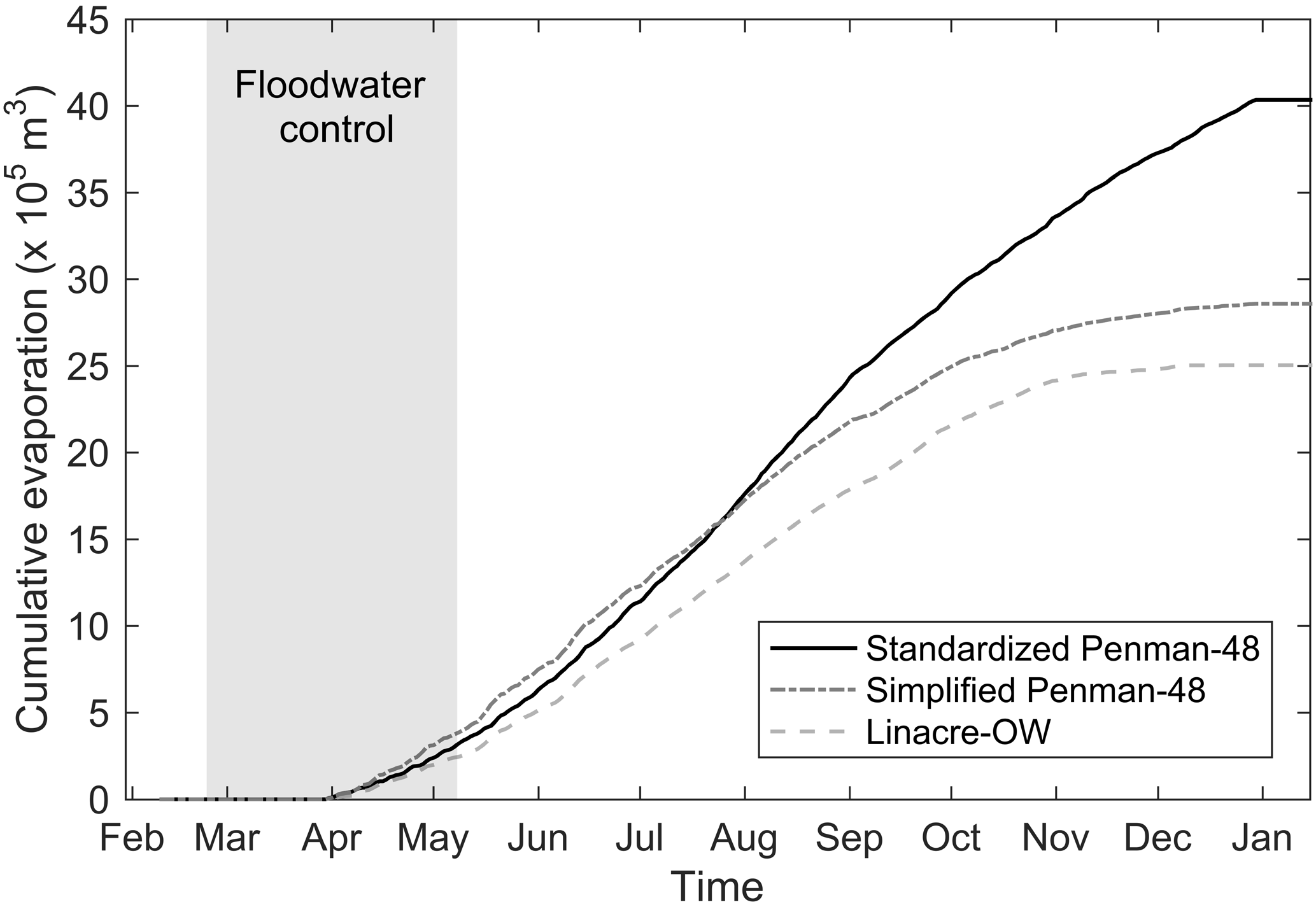
Figure C1Cumulative evaporative fluxes from lake A via the standardized Penman-48, simplified Penman-48 (Valiantzas, 2006), and Linacre-OW (Linacre, 1977) equations.
D1 Estimation of the water surface temperature based on the equilibrium method (de Bruin, 1982)
The water surface temperature (T) was estimated via the equilibrium method presented by de Bruin (1982) because no continuous measurements were available. This model is based on the assumption of a well-mixed surface body and was developed from standard land-based weather data. It was tested on two adjacent reservoirs in the Netherlands, with average depths of 5 and 15 m, respectively. Similar to de Bruin (1982), we used the 10 d mean values because we are interested in the annual variations in the water temperature. Moreover, the 10 d mean values were found to better simulate the observed water surface temperature. The difference between the observed and modelled water temperature is typically ≤1 ∘C, except in July and December where discrepancies of up to 5 ∘C were observed (Fig. D1). This is likely because lake A develops a thermal stratification over summertime and in wintertime. Potential uncertainties in isotopic mass balance models due to stratification in lakes up to 35 m were previously described and discussed by Gibson et al. (2017, 2019). They reported that sampling methods and lake stratification can lead to volume-dependent bias in the water balance partition. In this study, not accounting fully for thermal stratification will lead to overestimation of evaporation fluxes, and groundwater exchange will potentially be underestimated.
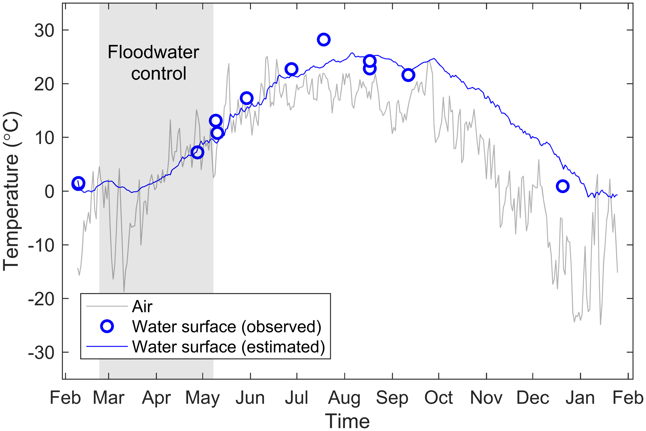
Figure D1Temporal evolution of air temperature and observed and estimated water surface temperatures at lake A. Water surface temperature estimations were computed according to the equilibrium method described by de Bruin (1982).
E1 Isotopic composition along vertical profiles in lake A
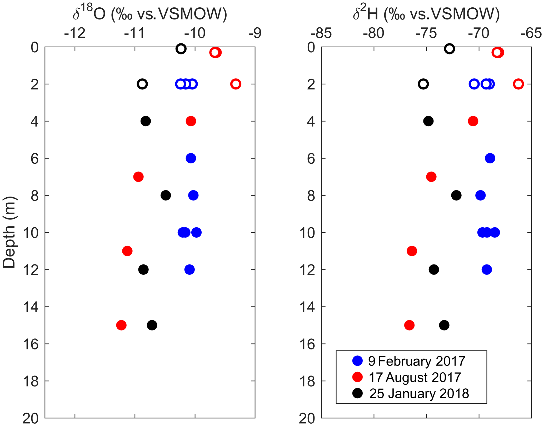
Figure E1Isotopic composition of lake A water samples against depth on 9 February 2017, 17 August 2017, and 25 January 2018. The hollow circles and solid circles represent samples collected at ≤2 and >2 m depth, respectively.
F1 Results of the sensitivity analysis for reference scenarios A and B
See Tables F1 and F2.
Table F1Sensitivity analysis on the input parameters of the isotopic mass balance model. Q is the output flux from lake A, I the input flux, and tf the mean flushing time by groundwater.
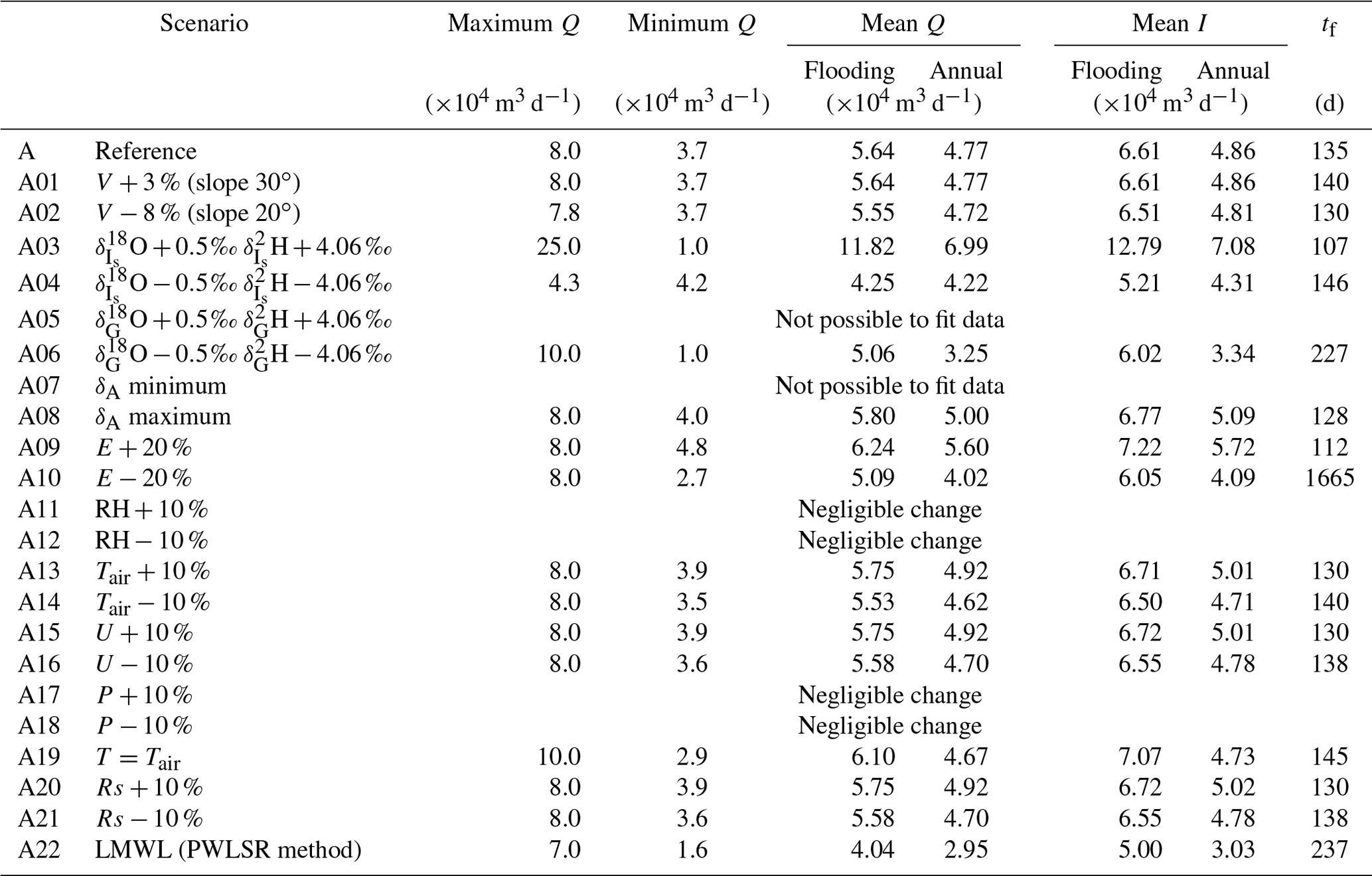
Table F2Sensitivity analysis on the input parameters of the isotopic mass balance model for the reference scenario B. Q is the output flux from lake A, I the input flux, and tf the mean flushing time by groundwater.
The code and data are available upon request to the corresponding author.
JMD, FB, and PB conceptualized the paper. JMD, FB, PB, and JG developed the methodology and contributed to the writing of the paper, with JMD writing the original draft and PB, FB, and JG reviewing and editing the paper. JMD also curated the data, led the investigation, and visualized the project. FB and PB supervised, with PB also taking responsibility for the funding acquisition and project administration.
The authors declare that they have no conflict of interest.
Publisher's note: Copernicus Publications remains neutral with regard to jurisdictional claims in published maps and institutional affiliations.
The authors are grateful to the town of Sainte-Marthe-sur-le-Lac and Gilbert Rybicki, who allowed access and water sampling on their property. Thanks go to the students (Marc Patenaude, Tom Crouzal, and Rose-Anne Farley, just to name a few) who participated in the fieldwork. We also gratefully acknowledge Jean-François Hélie and Marina Tcaci, from Geotop-UQAM, and Manon Leduc and Jérôme Leroy, from the Laboratoire de géochimie de Polytechnique Montréal. We thank Chani Welch, Bruno Hamelin, Michael Ronsen, and two anonymous reviewers for their thorough reading of the paper and their many insightful comments and suggestions which helped to improve the paper.
This research has been supported by the town of Sainte-Marthe-sur-le-Lac and the Natural Sciences and Engineering Research Council of Canada (grant nos. CRSNG-RDCPJ: 523095-17 and CRSNG-RGPIN-2016-06780).
This paper was edited by Genevieve Ali and reviewed by Bruno Hamelin, Chani Welch, and two anonymous referees.
Ageos: Drinking water supply: Application for an authorization under Section 31 of Groundwater Catchment Regulation: Hydrogeological expert report, 2010-723, volume 1 de 2, AGEOS, Brossard, QC, Canada, 2010.
Ageos: Drinking water supply: Monitoring of piezometric fluctuations in the water table and lake levels: Period from April 27, 2012 to December 17, 2015: Annual Report 2015, AGEOS, Brossard, QC, Canada, 42 pp., 2016.
Aissia, M. A. B., Chebana, F., Ouarda, T. B. M. J., Roy, L., Desrochers, G., Chartier, I., and Robichaud, É.: Multivariate analysis of flood characteristics in a climate change context of the watershed of the Baskatong reservoir, Province of Québec, Canada, Hydrol. Process., 26, 130–142, https://doi.org/10.1002/hyp.8117, 2012.
Arnoux, M., Barbecot, F., Gibert-Brunet, E., Gibson, J., and Noret, A.: Impacts of changes in groundwater recharge on the isotopic composition and geochemistry of seasonally ice-covered lakes: insights for sustainable management, Hydrol. Earth Syst. Sci., 21, 5875–5889, https://doi.org/10.5194/hess-21-5875-2017, 2017a.
Arnoux, M., Barbecot, F., Gibert-Brunet, E., Gibson, J., Rosa, E., Noret, A., and Monvoisin, G.: Geochemical and isotopic mass balances of kettle lakes in southern Quebec (Canada) as tools to document variations in groundwater quantity and quality, Environ. Earth Sci., 76, 106, https://doi.org/10.1007/s12665-017-6410-6, 2017b.
Arnoux, M., Gibert-Brunet, E., Barbecot, F., Guillon, S., Gibson, J., and Noret, A.: Interactions between groundwater and seasonally ice-covered lakes: Using water stable isotopes and radon-222 multilayer mass balance models, Hydrol. Process., 31, 2566–2581, https://doi.org/10.1002/hyp.11206, 2017c.
Barbecot, F., Guillon, S., Pili, E., Larocque, M., Gibert-Brunet, E., Hélie, J.-F., Noret, A., Plain, C., Schneider, V., Mattei, A., and Meyzonnat, G.: Using Water Stable Isotopes in the Unsaturated Zone to Quantify Recharge in Two Contrasted Infiltration Regimes, Vadose Zone J., 17, 170170, https://doi.org/10.2136/vzj2017.09.0170, 2018.
Barbecot, F., Larocque, M., and Horoi, V.: Research infrastructure on groundwater recharge, in: Isotopic composition of precipitation, Saint-Bruno, QC, Canada, 2019.
Baudron, P., Barbecot, F., Gillon, M., Aróstegui, J. L. G., Travi, Y., Leduc, C., Castillo, F. G., and Martinez-Vicente, D.: Assessing Groundwater Residence Time in a Highly Anthropized Unconfined Aquifer Using Bomb Peak 14C and Reconstructed Irrigation Water 3H, Radiocarbon, 53, 933–1006, https://doi.org/10.2458/azu_js_rc.55.16396, 2013.
Biehler, A., Chaillou, G., Buffin-Bélanger, T., and Baudron, P.: Hydrological connectivity in the aquifer–river continuum: impact of river stages on the geochemistry of groundwater floodplains, J. Hydrol., 590, 125379, https://doi.org/10.1016/j.jhydrol.2020.125379, 2020.
Bocanegra, E., Quiroz Londoño, O. M., Martínez, D. E., and Romanelli, A.: Quantification of the water balance and hydrogeological processes of groundwater–lake interactions in the Pampa Plain, Argentina, Environ. Earth Sci., 68, 2347–2357, https://doi.org/10.1007/s12665-012-1916-4, 2013.
Brock, B. E., Wolfe, B. B., and Edwards, T. W. D.: Characterizing the Hydrology of Shallow Floodplain Lakes in the Slave River Delta, NWT, Canada, Using Water Isotope Tracers, Arct. Antarct. Alp. Res., 39, 388–401, https://doi.org/10.1657/1523-0430(06-026)[BROCK]2.0.CO;2, 2007.
Centre d'Expertise Hydrique du Québec: Délimitation des bassins versants correspondant aux stations hydrométriques ouvertes et fermées, available at: https://www.cehq.gouv.qc.ca/hydrometrie/index.htm, last access: 18 December 2019.
Centre d'Expertise Hydrique du Québec: Niveau d'eau à la station 043108 (Lac des Deux Montagnes), available at: http://cehq.gouv.qc.ca/depot/historique_donnees_instantanees/043108_N_2017.txt (last access: 18 August 2019), 2020.
Clark, I.: Groundwater Geochemistry and Isotopes, CRC Press Taylor & Francis Group, Boca Raton, FL, 2015.
Craig, H. and Gordon, L. I.: Deuterium and oxygen 18 variations in the ocean and the marine atmosphere, in: Stable isotopes in oceanographic studies and paleotemperatures, edited by: Tongiorgi, E., Lab. Geologia Nucleare, Pisa, 9–130, 1965.
Cumming, G. S., Barnes, G., Perz, S., Schmink, M., Sieving, K. E., Southworth, J., Binford, M., Holt, R. D., Stickler, C., and Van Holt, T.: An Exploratory Framework for the Empirical Measurement of Resilience, Ecosystems, 8, 975–987, https://doi.org/10.1007/s10021-005-0129-z, 2005.
Cunha, D. G. F., Sabogal-Paz, L. P., and Dodds, W. K.: Land use influence on raw surface water quality and treatment costs for drinking supply in São Paulo State (Brazil), Ecol. Eng., 94, 516–524, https://doi.org/10.1016/j.ecoleng.2016.06.063, 2016.
de Bruin, H. A. R.: Temperature and energy balance of a water reservoir determined from standard weather data of a land station, J. Hydrol., 59, 261–274, https://doi.org/10.1016/0022-1694(82)90091-9, 1982.
Delpla, I., Jung, A. V., Baures, E., Clement, M., and Thomas, O.: Impacts of climate change on surface water quality in relation to drinking water production, Environ. Int., 35, 1225–1233, https://doi.org/10.1016/j.envint.2009.07.001, 2009.
Dibike, Y. B. and Coulibaly, P.: Hydrologic impact of climate change in the Saguenay watershed: comparison of downscaling methods and hydrologic models, J. Hydrol., 307, 145–163, https://doi.org/10.1016/j.jhydrol.2004.10.012, 2005.
Edwards, T. W. D., Wolfe, B. B., Gibson, J. J., and Hammarlund, D.: Use of water isotope tracers in high latitude hydrology and paleohydrology, in: Long-term environmental change in Arctic and Antarctic Lakes, developments in paleoenvironmental research, edited by: Pienitz, R., Douglas, M., and Smol, J. P., Springer, Dordrecht, the Netherlands, 187–207, 2004.
Falcone, M.: Assessing hydrological processes controlling the water balance of lakes in the Peace-Athabasca Delta, Alberta, Canada using water isotope tracers, UWSpace, University of Waterloo, Waterloo, Ontario, Canada, available at: http://hdl.handle.net/10012/3081 (last access: 14 July 2020), 2007.
Gibson, J. J.: Short-term evaporation and water budget comparisons in shallow Arctic lakes using non-steady isotope mass balance, J. Hydrol., 264, 242–261, https://doi.org/10.1016/S0022-1694(02)00091-4, 2002.
Gibson, J. J., Edwards, T. W. D., Bursey, G. G., and Prowse, T. D.: Estimating Evaporation Using Stable Isotopes: Quantitative Results and Sensitivity Analysis for Two Catchments in Northern Canada: Paper presented at the 9th Northern Res. Basin Symposium/Workshop (Whitehorse/Dawson/Inuvik, Canada – August 1992), Hydrol. Res., 24, 79–94, https://doi.org/10.2166/nh.1993.0015, 1993.
Gibson, J. J., Birks, S. J., and Yi, Y.: Stable isotope mass balance of lakes: a contemporary perspective, Quaternary Sci. Rev., 131, 316–328, https://doi.org/10.1016/j.quascirev.2015.04.013, 2015.
Gibson, J. J., Birks, S. J., Yi, Y., Moncur, M. C., and McEachern, P. M.: Stable isotope mass balance of fifty lakes in central Alberta: Assessing the role of water balance parameters in determining trophic status and lake level, J. Hydrol.: Reg. Stud., 6, 13–25, https://doi.org/10.1016/j.ejrh.2016.01.034, 2016.
Gibson, J. J., Birks, S. J., Jeffries, D., and Yi, Y.: Regional trends in evaporation loss and water yield based on stable isotope mass balance of lakes: The Ontario Precambrian Shield surveys, J. Hydrol., 544, 500–510, https://doi.org/10.1016/j.jhydrol.2016.11.016, 2017.
Gibson, J. J., Yi, Y., and Birks, S. J.: Isotopic tracing of hydrologic drivers including permafrost thaw status for lakes across Northeastern Alberta, Canada: A 16-year, 50-lake assessment, J. Hydrol.: Reg. Stud., 26, 100643, https://doi.org/10.1016/j.ejrh.2019.100643, 2019.
Gonfiantini, R.: Chapter 3 – Environmental Isotopes In Lake Studies, in: The Terrestrial Environment, B, edited by: Fritz, P. and Fontes, J. C., Elsevier, Amsterdam, 113–168, 1986.
Gran, G.: Determination of the equivalence point in potentiometric titrations. Part II, Analyst, 77, 661–671, https://doi.org/10.1039/AN9527700661, 1952.
Haig, H. A., Hayes, N. M., Simpson, G. L., Yi, Y., Wissel, B., Hodder, K. R., and Leavitt, P. R.: Comparison of isotopic mass balance and instrumental techniques as estimates of basin hydrology in seven connected lakes over 12 years, J. Hydrol., 6, 100046, https://doi.org/10.1016/j.hydroa.2019.100046, 2020.
Herczeg, A. L., Leaney, F. W., Dighton, J. C., Lamontagne, S., Schiff, S. L., Telfer, A. L., and English, M. C.: A modern isotope record of changes in water and carbon budgets in a groundwater-fed lake: Blue Lake, South Australia, Limnol. Oceanogr., 48, 2093–2105, https://doi.org/10.4319/lo.2003.48.6.2093, 2003.
Holtz, R. D. and Kovacs, W. D.: An Introduction to Geotechnical Engineering, Montreal, Canada, 832 pp., 1981.
Horita, J. and Wesolowski, D. J.: Liquid-vapor fractionation of oxygen and hydrogen isotopes of water from the freezing to the critical temperature, Geochim. Cosmochim. Ac., 58, 3425–3437, https://doi.org/10.1016/0016-7037(94)90096-5, 1994.
Horita, J., Rozanski, K., and Cohen, S.: Isotope effects in the evaporation of water: a status report of the Craig–Gordon model, Isotop. Environ. Health Stud., 44, 23–49, https://doi.org/10.1080/10256010801887174, 2008.
Hughes, C. E. and Crawford, J.: A new precipitation weighted method for determining the meteoric water line for hydrological applications demonstrated using Australian and global GNIP data, J. Hydrol., 464–465, 344–351, https://doi.org/10.1016/j.jhydrol.2012.07.029, 2012.
IAEA/WMO: Global Network of Isotopes in Precipitation, The GNIP Database, available at: https://nucleus.iaea.org/wiser (last access: 20 September 2019), 2018.
Isokangas, E., Rozanski, K., Rossi, P. M., Ronkanen, A. K., and Kløve, B.: Quantifying groundwater dependence of a sub-polar lake cluster in Finland using an isotope mass balance approach, Hydrol. Earth Syst. Sci., 19, 1247–1262, https://doi.org/10.5194/hess-19-1247-2015, 2015.
Jasechko, S., Wassenaar, L. I., and Mayer, B.: Isotopic evidence for widespread cold-season-biased groundwater recharge and young streamflow across central Canada, Hydrol. Process., 31, 2196–2209, https://doi.org/10.1002/hyp.11175, 2017.
Jeppesen, E., Meerhoff, M., Davidson, T. A., Trolle, D., Sondergaard, M., Lauridsen, T. L., Beklioglu, M., Brucet Balmaña, S., Volta, P., and González-Bergonzoni, I.: Climate change impacts on lakes: an integrated ecological perspective based on a multi-faceted approach, with special focus on shallow lakes, J. Limnol., 73, 88–111, https://doi.org/10.4081/jlimnol.2014.844, 2014.
Jones, M. D., Cuthbert, M. O., Leng, M. J., McGowan, S., Mariethoz, G., Arrowsmith, C., Sloane, H. J., Humphrey, K. K., and Cross, I.: Comparisons of observed and modelled lake δ18O variability, Quaternary Sci. Rev., 131, 329–340, https://doi.org/10.1016/j.quascirev.2015.09.012, 2016.
Kløve, B., Ala-aho, P., Bertrand, G., Boukalova, Z., Ertürk, A., Goldscheider, N., Ilmonen, J., Karakaya, N., Kupfersberger, H., Kvœrner, J., Lundberg, A., Mileusnić, M., Moszczynska, A., Muotka, T., Preda, E., Rossi, P., Siergieiev, D., Šimek, J., Wachniew, P., Angheluta, V., and Widerlund, A.: Groundwater dependent ecosystems. Part I: Hydroecological status and trends, Environ. Sci. Policy, 14, 770–781, https://doi.org/10.1016/j.envsci.2011.04.002, 2011.
Lerner, D. N. and Harris, B.: The relationship between land use and groundwater resources and quality, Land Use Policy, 26, S265–S273, https://doi.org/10.1016/j.landusepol.2009.09.005, 2009.
Linacre, E. T.: A simple formula for estimating evaporation rates in various climates, using temperature data alone, Agricult. Meteorol., 18, 409–424, https://doi.org/10.1016/0002-1571(77)90007-3, 1977.
Masse-Dufresne, J., Baudron, P., Barbecot, F., Patenaude, M., Pontoreau, C., Proteau-Bedard, F., Menou, M., Pasquier, P., Veuille, S., and Barbeau, B.: Anthropic and Meteorological Controls on the Origin and Quality of Water at a Bank Filtration Site in Canada, Water, 11, 2510, https://doi.org/10.3390/w11122510, 2019.
Masse-Dufresne, J., Baudron, P., Barbecot, F., Pasquier, P., and Barbeau, B.: Optimizing short time-step monitoring and management strategies using environmental tracers at flood-affected bank filtration sites, Sci. Total Environ., 750, 141429, https://doi.org/10.1016/j.scitotenv.2020.141429, 2021.
McJannet, D. L., Webster, I. T., and Cook, F. J.: An area-dependent wind function for estimating open water evaporation using land-based meteorological data, Environ. Model. Softw., 31, 76-83, https://doi.org/10.1016/j.envsoft.2011.11.017, 2012.
MDDELCC: Portrait sommaire du bassin versant de la rivière des Outaouais, available at: http://www.mddelcc.gouv.qc.ca/eau/bassinversant/bassins/outaouais/portrait-sommaire.pdf (last access: 5 September 2019), 2015.
Minville, M., Brissette, F., and Leconte, R.: Uncertainty of the impact of climate change on the hydrology of a nordic watershed, J. Hydrol., 358, 70–83, https://doi.org/10.1016/j.jhydrol.2008.05.033, 2008.
Monsen, N. E., Cloern, J. E., Lucas, L. V., and Monismith, S. G.: A comment on the use of flushing time, residence time, and age as transport time scales, Limnol. Oceanogr., 47, 1545–1553, https://doi.org/10.4319/lo.2002.47.5.1545, 2002.
Mueller, H., Hamilton, D. P., and Doole, G. J.: Evaluating services and damage costs of degradation of a major lake ecosystem, Ecosyst. Serv., 22, 370–380, https://doi.org/10.1016/j.ecoser.2016.02.037, 2016.
O'Neil, J. R.: Hydrogen and oxygen isotope fractionation between ice and water, J. Phys. Chem., 72, 3683–3684, https://doi.org/10.1021/j100856a060, 1968.
Patenaude, M., Baudron, P., Labelle, L., and Masse-Dufresne, J.: Evaluating Bank-Filtration Occurrence in the Province of Quebec (Canada) with a GIS Approach, Water, 12, 662, https://doi.org/10.3390/w12030662, 2020.
Pazouki, P., Prevost, M., McQuaid, N., Barbeau, B., de Boutray, M. L., Zamyadi, A., and Dorner, S.: Breakthrough of cyanobacteria in bank filtration, Water Res., 102, 170–179, https://doi.org/10.1016/j.watres.2016.06.037, 2016.
Petermann, E., Gibson, J. J., Knöller, K., Pannier, T., Weiß, H., and Schubert, M.: Determination of groundwater discharge rates and water residence time of groundwater-fed lakes by stable isotopes of water (18O, 2H) and radon (222Rn) mass balances, Hydrol. Process., 32, 805–816, https://doi.org/10.1002/hyp.11456, 2018.
Rosa, E., Hillaire-Marcel, C., Hélie, J.-F., and Myre, A.: Processes governing the stable isotope composition of water in the St. Lawrence river system, Canada, Isotop. Environ. Health Stud., 52, 370–379, https://doi.org/10.1080/10256016.2015.1135138, 2016.
Rosen, M. R.: The Influence of Hydrology on Lacustrine Sediment Contaminant Records, in: Environmental Contaminants: Using natural archives to track sources and long-term trends of pollution, edited by: Blais, J. M., Rosen, M. R., and Smol, J. P., Springer Netherlands, Dordrecht, 5–33, 2015.
Rosenberry, D. O., Lewandowski, J., Meinikmann, K., and Nützmann, G.: Groundwater – the disregarded component in lake water and nutrient budgets. Part 1: effects of groundwater on hydrology, Hydrol. Process., 29, 2895–2921, https://doi.org/10.1002/hyp.10403, 2015.
Roy, L., Leconte, R., Brissette, F. P., and Marche, C.: The impact of climate change on seasonal floods of a southern Quebec River Basin, Hydrol. Process., 15, 3167–3179, https://doi.org/10.1002/hyp.323, 2001.
Salinger, M. J.: Climate Variability and Change: Past, Present and Future – An Overview, Climatic Change, 70, 9–29, https://doi.org/10.1007/s10584-005-5936-x, 2005.
Scanlon, B. R., Reedy, R. C., Stonestrom, D. A., Prudic, D. E., and Dennehy, K. F.: Impact of land use and land cover change on groundwater recharge and quality in the southwestern US, Global Change Biol., 11, 1577–1593, https://doi.org/10.1111/j.1365-2486.2005.01026.x, 2005.
Schallenberg, M., de Winton, M. D., Verburg, P., Kelly, D. J., Hamill, K. D., and Hamilton, D. P.: Ecosystem services of lakes, in: Ecosystem services in New Zealand: conditions and trends, edited by: Dymond, J. R., Manaaki Whenua Press, Lincoln, New Zealand, 203–225, 2013.
Teufel, B., Sushama, L., Huziy, O., Diro, G. T., Jeong, D. I., Winger, K., Garnaud, C., de Elia, R., Zwiers, F. W., Matthews, H. D., and Nguyen, V. T. V.: Investigation of the mechanisms leading to the 2017 Montreal flood, Clim. Dynam., 52, 4193–4206, https://doi.org/10.1007/s00382-018-4375-0, 2019.
Turner, K. W., Wolfe, B. B., and Edwards, T. W. D.: Characterizing the role of hydrological processes on lake water balances in the Old Crow Flats, Yukon Territory, Canada, using water isotope tracers, J. Hydrol., 386, 103–117, https://doi.org/10.1016/j.jhydrol.2010.03.012, 2010.
Valiantzas, J. D.: Simplified versions for the Penman evaporation equation using routine weather data, J. Hydrol., 331, 690–702, https://doi.org/10.1016/j.jhydrol.2006.06.012, 2006.
Walsh, J. R., Carpenter, S. R., and Vander Zanden, M. J.: Invasive species triggers a massive loss of ecosystem services through a trophic cascade, P. Natl. Acad. Sci. USA, 113, 4081, https://doi.org/10.1073/pnas.1600366113, 2016.
Welch, C., Smith, A. A., and Stadnyk, T. A.: Linking physiography and evaporation using the isotopic composition of river water in 16 Canadian boreal catchments, Hydrol. Process., 32, 170–184, https://doi.org/10.1002/hyp.11396, 2018.
Wheaton, E., Koshida, G., Bonsal, B., Johnston, T., Richards, W., and Wittrock, V.: Agricultural Adaptation to Drought (ADA) in Canada: The Case of 2001 to 2002, SK Canada, Saskatoon, 1–14, 2007.
Wolfe, B. B., Karst-Riddoch, T. L., Hall, R. I., Edwards, T. W. D., English, M. C., Palmini, R., McGowan, S., Leavitt, P. R., and Vardy, S. R.: Classification of hydrological regimes of northern floodplain basins (Peace–Athabasca Delta, Canada) from analysis of stable isotopes (δ18O, δ2H) and water chemistry, Hydrol. Process., 21, 151–168, https://doi.org/10.1002/hyp.6229, 2007.
Zimmermann, U.: Determination by stable isotopes of underground inflow and outflow and evaporation of young artificial groundwater lakes, in: Isotopes in lakes studies, IAEA, Vienna, Austria, 87–94, 1979.