Using Long Short-Term Memory networks to connect water table depth anomalies to precipitation anomalies over Europe

Many European countries rely on groundwater for public and industrial water supply. Due to a scarcity of near-real-time water table depth (wtd) observations, establishing a spatially consistent groundwater monitoring system at the continental scale is a challenge. Hence, it is necessary to develop alternative methods for estimating wtd anomalies (wtd_a) using other hydrometeorological observations routinely available near real time. In this work, we explore the potential of Long Short-Term Memory (LSTM) networks for producing monthly wtd_a using monthly precipitation anomalies (pr_a) as input. LSTM networks are a special category of artificial neural networks that are useful for detecting a long-term dependency within sequences, in our case time series, which is expected in the relationship between pr_a and wtd_a. In the proposed methodology, spatiotemporally continuous data were obtained from daily terrestrial simulations of the Terrestrial Systems Modeling Platform (TSMP) over Europe (hereafter termed the TSMP-G2A data set), with a spatial resolution of 0.11^∘, ranging from the years 1996 to 2016. The data were separated into a training set (1996–2012), a validation set (2013–2014), and a test set (2015–2016) to establish local networks at selected pixels across Europe. The modeled wtd_a maps from LSTM networks agreed well with TSMP-G2A wtd_a maps on spatially distributed dry and wet events, with 2003 and 2015 constituting drought years over Europe. Moreover, we categorized the test performances of the networks based on intervals of yearly averaged wtd, evapotranspiration (ET), soil moisture (θ), snow water equivalent (S_w), soil type (S_t), and dominant plant functional type (PFT). Superior test performance was found at the pixels with wtd < 3 m, ET > 200 mm, θ>0.15 m³ m⁻³, and S_w<10 mm, revealing a significant impact of the local factors on the ability of the networks to process information. Furthermore, results of the cross-wavelet transform (XWT) showed a change in the temporal pattern between TSMP-G2A pr_a and wtd_a at some selected pixels, which can be a reason for undesired network behavior. Our results demonstrate that LSTM networks are useful for producing high-quality wtd_a based on other hydrometeorological data measured and predicted at large scales, such as pr_a. This contribution may facilitate the establishment of an effective groundwater monitoring system over Europe that is relevant to water management.

1 Introduction

Groundwater is an essential natural resource, accounting for about 30 % of the fresh water on Earth (Perlman, 2013), and sustains various domestic, agricultural, industrial, and environmental uses due to its widespread availability and limited vulnerability to pollution (Naghibi et al., 2016; Tian et al., 2016). According to the report of the European Environment Agency (EEA) in 1999, groundwater comprises over 50 % of the public water supply in most European countries (EEA, 1999). Groundwater systems are dynamic and adapt continuously to natural and anthropogenic stresses (Kenda et al., 2018). However, they have been affected in recent years as a consequence of frequent extreme weather conditions, e.g., severe droughts and human overexploitation. Thus, effective and efficient groundwater management, especially under drought conditions, is required at the European scale to maintain environmental and socioeconomic sustainability.

Drought is characterized as the costliest natural hazard worldwide, resulting in significant societal, economic, and ecological impacts (Wilhite, 2000). The report of the EEA in 2016 demonstrated that drought had become a recurrent feature of the European climate; more droughts have occurred in some European countries than in the past, and their severity has also increased (EEA, 2016). Recent severe heat wave events in Europe occurred in 2003, 2015, and 2018, which led to several drought events covering most of the European continent (Norris, 2018). Groundwater drought is a specific type of drought, impacting several important drought-sensitive sectors, such as drinking water supply and irrigation (Van Loon et al., 2017). Hence, groundwater monitoring is ultimately indispensable over the European continent.

Effective groundwater monitoring requires accurate information on groundwater dynamics in space and time. One crucial variable for characterizing groundwater dynamics is the water table depth anomaly (wtd_a), reflecting anomalies in groundwater storage (Zhao et al., 2020), which is a key variable in groundwater drought analysis. The wtd_a is the deviation of the wtd value from the climatological average for a specified time period normalized by the climatological standard deviation and can serve as a measure of groundwater drought. Commonly, wtd observations are measured in situ in observation wells. However, to date, it is still a challenge to obtain near-real-time spatially continuous wtd observations over Europe (Van Loon et al., 2017; Bloomfield et al., 2018), and available data sets often suffer from uncertainties originating from unknown well bore and well installation specifics. Therefore, an alternative (indirect) method is needed to produce reliable, area-wide wtd_a information over Europe.

Indirect methods rely on measurements of one (or more) hydrometeorological variable related to wtd via physical processes in the water cycle, such as infiltration and percolation. The precipitation anomaly (pr_a) is the most common variable used to model wtd_a, for which the calculation method is the same as wtd_a but based on precipitation (P). P is connected with groundwater via the process of percolation through soil layers. Thus, depending on evapotranspiration (ET) and the thickness of the vadose zone, a lag exists in the response of groundwater to P. A considerable number of studies linked the accumulation of pr_a over extended timescales (e.g., 6 or 12 months) to wtd_a, often applying the Standardized Precipitation Index (SPI) and the Standardized Precipitation Evapotranspiration Index (SPEI) to represent wtd_a (e.g., SPI: McKee et al., 1993; Thomas et al., 2015; SPEI: Vicente-Serrano et al., 2010; Van Loon et al., 2017). In these studies, equal weighting was assigned to the meteorological input in the derivation of the drought indices.

As an alternative, artificial neural networks (ANNs) are able to account for non-uniformly weighted, temporally lagged contributions of pr_a to wtd_a, potentially providing more robust prediction models. ANNs are one of the most widely used machine learning methods that have been inspired by biological neural systems, with many interconnected information processing units (i.e., neurons; Haykin, 2009; Ma et al., 2019). ANNs adapt learnable parameters (i.e., weights and biases) in the links between neurons to achieve an appropriate input–output mapping based on observed data; this is also for complex nonlinear relationships. ANNs are not easily affected by input noise and are able to readjust their parameters when new information is included. More importantly, compared to physically based models, they necessitate little background knowledge, reducing the requirements for human involvement and expertise, thus enabling rapid hypothesis testing (Govindaraju, 2000; Shen, 2018; Sun and Scanlon, 2019).

Feedforward neural networks (FFNNs, also termed multilayer perceptrons in some of the literature) and their variants are commonly used ANNs for groundwater level modeling in previous studies (e.g., Yang et al., 1997; Nayak et al., 2006; Adamowski and Chan, 2011; Yoon et al., 2011; Mohanty et al., 2015; Gong et al., 2016; Sun et al., 2016). One major drawback of FFNNs is that they cannot preserve previous information, resulting in inefficiencies in handling sequential data (J. Zhang et al., 2018; Supreetha et al., 2020). To leverage the performance of FFNNs, the delay time in the network response needs to be estimated in advance.

Recurrent neural networks (RNNs) are a special type of ANN mainly designed for sequential data analysis. Through loops in their hidden layers, the information generated in the past flows back to neurons as the input of new computing processes (Karim and Rivera, 1992). Due to the ability to store information traveling through, RNNs can avoid the aforementioned preprocessing step of FFNNs and can, thereby, solve sequential data problems more efficiently. However, standard RNNs suffer from the exploding and vanishing gradient issues and often fail to exploit long-term dependencies between sequences, which is expected in the response of wtd_a to pr_a. These issues can be overcome by a variant of standard RNNs named Long Short-Term Memory (LSTM) networks (Supreetha et al., 2020). Although RNNs have been employed extensively in other science fields, particularly in natural language processing (D. Zhang et al., 2018), their application in hydrology is still in its infancy and has only recently received increasing attention (e.g., Kratzert et al., 2018; Shen, 2018; J. Zhang et al., 2018; Le et al., 2019; Sahoo et al., 2019). Thus, limited studies have been conducted to estimate groundwater fluctuations using RNNs, especially with LSTM networks.

The consistency of the temporal pattern between input and target variables is a prerequisite for the good performance of ANNs, including LSTM networks. Cross-wavelet transform (XWT) is a useful tool for visualizing the pattern changes between input and target variables, aiming to extract similarities of two time series in time and frequency. The technique has been applied for time–frequency analysis in many publications (e.g., Adamowski, 2008; Prokoph and El Bilali, 2008; Banerjee and Mitra, 2014).

In this study, we utilized spatiotemporally continuous pr_a and wtd_a from integrated hydrologic simulation results of the Terrestrial Systems Modeling Platform (TSMP) over Europe (hereafter termed the TSMP-G2A data set and introduced in Sect. 2.4) in combination with LSTM networks to capture the time-varying and time-lagged relationship between pr_a and wtd_a in order to obtain reliable prediction models at the individual pixel level. The impact of local factors on the network behavior was also investigated, and the local factors studied were yearly averaged wtd, ET, soil moisture (θ), snow water equivalent (S_w), and soil type (S_t) and dominant plant functional type (PFT). In addition, we implemented XWT on both TSMP-G2A pr_a and wtd_a series for time–frequency analysis to gain insight into the internal characteristics of the obtained networks.

This paper is organized as follows: in Sect. 2 (Methodology), we first present a conceptual model of groundwater balance to theoretically derive the relationship between pr_a and wtd_a and then briefly introduce the architecture of the proposed LSTM networks and continuous and cross-wavelet transform. This is then followed by detailed information on our study area and data set, as well as a generic workflow to construct local LSTM networks at selected pixels over Europe. Section 3 (Results and discussion) shows reproduced wtd_a maps for groundwater drought analysis, discusses the impact of local factors on the network behaviors, and investigates the network performances at the local scale, before completing the paper with Sect. 4 (Summary and conclusions).

2 Methodology

LSTM networks were applied to estimate monthly wtd_a over the European continent, using monthly pr_a as input. We constructed the networks at the individual pixels and analyzed temporal patterns between TSMP-G2A pr_a and wtd_a using XWT. In this section, we briefly recall the conceptual model of groundwater balance, introduce the principle of LSTM networks and the application of XWT, and describe the study area and data set before presenting a universal workflow to establish the proposed LSTM networks locally at selected pixels.

2.1 Conceptual model of groundwater balance

The subsurface water balance can be described by a control volume that contains the vadose zone and an unconfined aquifer that is closed at the bottom (Fig. 1). Note that areas with surface water are not taken into account in this study, and the impact of anthropogenic activities such as groundwater abstraction is neglected. Flows in and out of the control volume are P and ET across the land surface and lateral flows in the subsurface. These flows are balanced by changes in the water stored in the vadose zone and the unconfined aquifer.

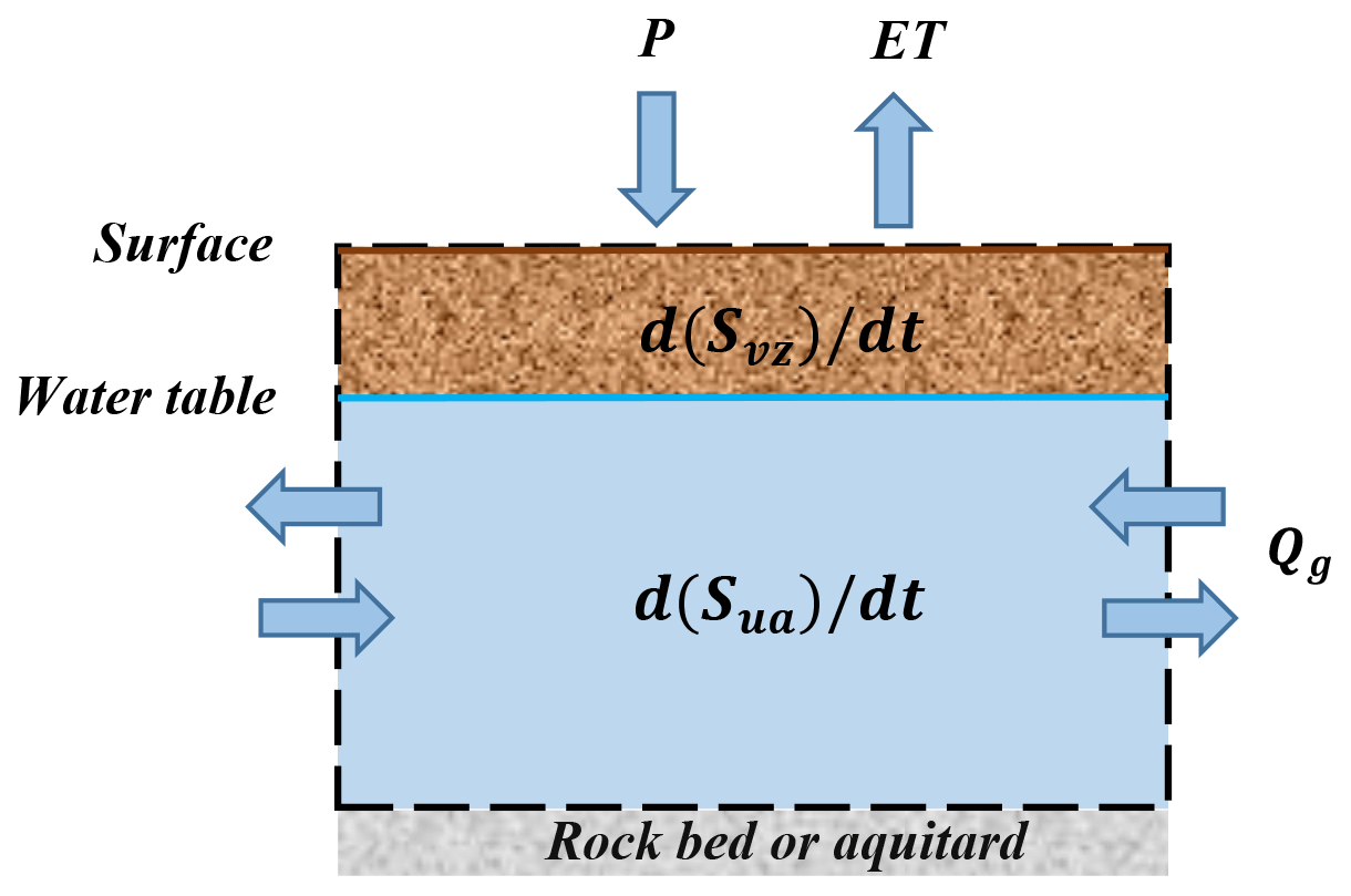
Figure 1 Conceptual model of groundwater balance over a control volume (after Maxwell, 2010). P is precipitation, ET is actual evapotranspiration, Q_g is the lateral groundwater flow, S_vz and S_ua are the water storages in the vadose zone and the unconfined aquifer, respectively, and t is time.

The groundwater balance equation for the conceptual model is given in Eq. (1) as follows:

$$\begin{array}{}\text{(1)}& \mathrm{d}\left(S_{\mathrm{vz}}\right)/\mathrm{d}t+\mathrm{d}\left(S_{\mathrm{ua}}\right)/\mathrm{d}t=P-\mathrm{ET}+{\mathit{Q}}_{\mathrm{g}}.\end{array}$$

Rearranging Eq. (1), will result in Eq. (2), as follows:

$$\begin{array}{}\text{(2)}& \mathrm{d}\left(S_{\mathrm{ua}}\right)/\mathrm{d}t=P-\mathrm{ET}+{\mathit{Q}}_{\mathrm{g}}-\mathrm{d}\left(S_{\mathrm{vz}}\right)/\mathrm{d}t,\end{array}$$

where P is precipitation (millimeters per month), ET is actual evapotranspiration (millimeters per month), and Q_g is the lateral groundwater flow (millimeters per month). S_vz and S_ua are the water storages in the vadose zone (millimeters) and the unconfined aquifer (millimeters), respectively, and t is time (months).

The term on the left-hand side and the first term on the right-hand side in Eq. (2) indicate an explicit relationship between the fluctuation of S_ua and P, providing the theoretical basis of this study. In the case of large continental watersheds (i.e., Q_g=0), the difference between P and ET is equal to the total variations in S_vz and S_ua. Note that we explicitly separated the water storage term of the vadose zone from the unconfined aquifer to highlight the transient impact of unsaturated storage on the relationship between $\mathrm{d}\left(S_{\mathrm{ua}}\right)/\mathrm{d}t$ and (P–ET).

2.2 Long Short-Term Memory networks

In this study, we employed LSTM networks with the same architecture of hidden neurons as in Gers et al. (2000), as shown in Fig. 2. As a category of RNNs, LSTM networks have loops in their hidden layers that facilitate hidden neurons to weigh not only new inputs but also earlier outputs internally for predictions. Hence, similar to other RNNs, they are considered to have memory. Compared with standard RNNs, LSTM networks add a constant error carousel (CEC) and three gates that are the input, forget, and output gates in their hidden neurons (see Fig. 2) in order to overcome the exploding and vanishing gradient issues. For a detailed description of the functions of these components, the reader is referred to Hochreiter and Schmidhuber (1997) and Gers et al. (2000). Benefiting from the interaction of these components, LSTM networks show great promise for studying long-term relationships between time series. They have the ability to capture dependencies over 1000 time steps, outperforming standard RNNs whose upper boundary of reliable performance is only 10 time steps (Hochreiter and Schmidhuber, 1997; Kratzert et al., 2018). The response of wtd_a to pr_a is expected to exhibit a long time lag, especially in case of deep aquifers, and thus, LSTM networks are an appropriate type of network to use here. In addition, compared with traditional physically based models, the proposed LSTM networks require less computational time and background knowledge to perform the simulations. Moreover, when the proposed LSTM networks are available, we only need the pr_a data to estimate wtd_a, which are available from bias-corrected operational forecasts and reanalysis data sets.

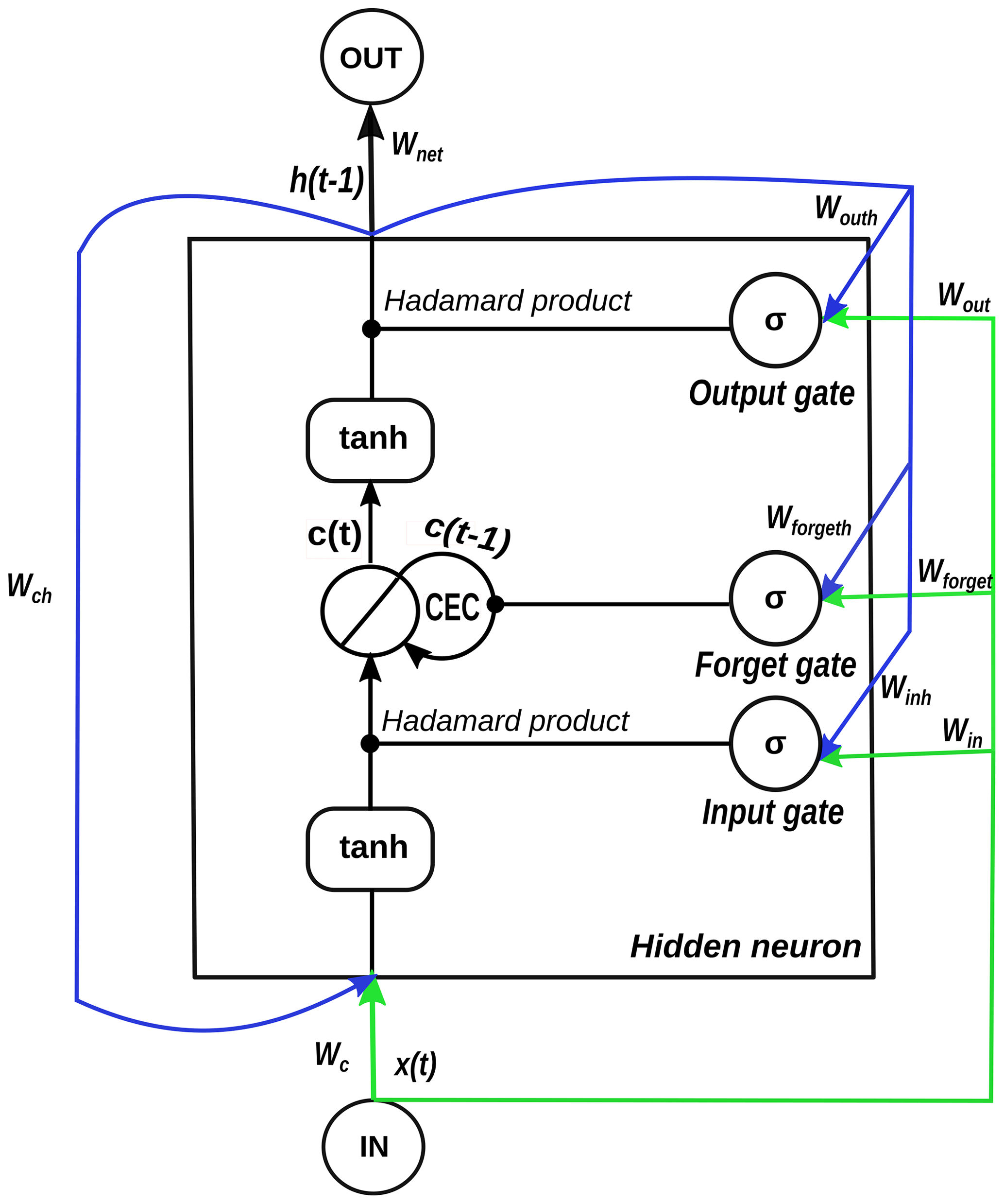
Figure 2 One hidden layer LSTM network with one hidden neuron. The green lines indicate the entry points of new inputs into the hidden neuron. The blue lines show the entry points of previous outputs into the hidden neuron, where w_* is the weight on a linkage, h(^*) is the output of the hidden neuron, x(t) is the input at the time step t, and c(^*) is the cell state of the constant error carousel (CEC). σ represents a sigmoid function of a gate, and tanh is a hyperbolic tangent function.

The procedure for processing inputs in hidden neurons of LSTM networks is as follows (Olah, 2015; Ma et al., 2019): (1) filter the information used for prediction from new inputs based on the result of the input gate, (2) filter the information to be remembered from the old CEC state according to the output of the forget gate, (3) update the CEC state using the results from the previous two steps, and (4) compute outputs of hidden neurons from the new CEC state and the results given by the output gate.

Figure 2 illustrates a one hidden layer LSTM network containing only one hidden neuron; the pseudocode is presented in Appendix A to detail how data are transferred in the given LSTM network. Owing to the limited data available at each pixel (i.e., a total of 252 time steps), we built small LSTM networks at the local scale with one input layer, one hidden layer, and one output layer. The network receives monthly pr_a from the input layer, processes it on the hidden layer, and finally generates monthly wtd_a from the output layer. The numbers of input and output neurons are determined by how many input and output variables are used in the derivation of the network. In the constructed LSTM networks, only one neuron is located on either the input or output layer, as the number of input or output variables is one. Thus, the complexity of the network only depends on the number of hidden neurons and, therefore, can vary by changing the number of hidden neurons. The architecture of a network plays an important role in its behavior when processing new data, and it can be a double-edged sword to apply a network with considerable hidden neurons. On the one hand, the bigger we allow a network to grow, the better it can learn from a given data set. On the other hand, a complex network easily captures unwanted patterns when it learns too much from the given data set, eliminating its ability to deal with previously unobserved information (Dawson and Wilby, 2001; Müller and Guido, 2017). This phenomenon is termed overfitting. Hence, it is crucial to identify the optimal number of hidden neurons and specify the appropriate structure of the network, which is the focus of the hyperparameter tuning described in Sect. 2.5.

2.3 Continuous and cross-wavelet transform

Continuous wavelet transform (CWT) is a type of wavelet transform useful for feature extraction (Grinsted et al., 2004). Given a mother wavelet ψ₀(η), with η being a dimensionless time parameter, the CWT of a time series $x_{n_{\mathrm{0}}}$ is formulated as the convolution of $x_{n_{\mathrm{0}}}$ and a scaled and translated form of ψ₀(η) as follows (Torrence and Compo, 1998):

$$\begin{array}{}\text{(3)}& W(s,n)=\sum _{n_{\mathrm{0}}=\mathrm{0}}^{N-\mathrm{1}}{x}_{n_{\mathrm{0}}}{\mathit{\psi }}^{*}\left[\left(n_{\mathrm{0}}-n\right)\mathit{\delta }t/s\right],\end{array}$$

where the asterisk (^*) signifies the complex conjugate, δt is the time step of $x_{n_{\mathrm{0}}}$, N is the total number of δt in $x_{n_{\mathrm{0}}}$, s is the wavelet scale, and n is the localized time index along which ψ₀(η) is translated. Here, the wavelet power is defined as $\left|W\right(s,n){|}^{\mathrm{2}}$.

The mother wavelet must be zero mean and localized in the time and frequency domains (Torrence and Compo, 1998). In this study, we applied the Morlet wavelet as the mother wavelet, defined as follows:

$$\begin{array}{}\text{(4)}& {\mathit{\psi }}_{\mathrm{0}}\left(\mathit{\eta }\right)={\mathit{\pi }}^{-\mathrm{1}/\mathrm{4}}{e}^{i{\mathit{\omega }}_{\mathrm{0}}\mathit{\eta }}{e}^{-{\mathit{\eta }}^{\mathrm{2}}/\mathrm{2}},\end{array}$$

where ω₀ is the dimensionless frequency, which is set as 6 here to acquire a good balance between time and frequency localization (Grinsted et al., 2004).

XWT is a method for locating common high power in the wavelet transforms of two time series. The XWT of two time series, $x_{n_{\mathrm{0}}}$ and $y_{n_{\mathrm{0}}}$, can be computed using the following (Grinsted et al., 2004):

$$\begin{array}{}\text{(5)}& W_{xy}(s,n)=W_x(s,n)W_y^{*}(s,n),\end{array}$$

where W_x(s,n) and W_y(s,n) are the CWT of the time series $x_{n_{\mathrm{0}}}$ and $y_{n_{\mathrm{0}}}$, respectively. The cross-wavelet power is calculated as $\left|W_{xy}\right(s,n\left)\right|$. However, directly using the cross-wavelet power gives biased results of the XWT analysis, so we applied $\left|W_{xy}\right(s,n\left)\right|/s$ proposed by Veleda et al. (2012) for correction. For detailed descriptions about CWT and XWT, the reader is referred to Torrence and Compo (1998), Grinsted et al. (2004), Prokoph and El Bilali (2008), and Veleda et al. (2012).

In this study, XWT is used as an independent and additional analysis tool to visualize the pattern in the pr_a–wtd_a relationship at the individual pixel level in time and frequency. In the XWT analyses, we focus on common, localized high-power frequency modes of ψ₀(η) in pr_a and wtd_a time series and the dynamics of the modes over time. Using the XWT analysis, we expect to clarify whether a changing pattern exists in the pr_a–wtd_a relationship during the study period and if it affects the network behavior. Moreover, by linking the results of the XWT analysis with the network outputs, we explore the impact of the amount and range of the frequency modes on the LSTM network performance in order to obtain insight into the internal operations of LSTM networks.

2.4 Study area and data set

We constructed the LSTM networks at individual pixels over eight hydrometeorologically different regions within Europe (Fig. 3), which are known as the PRUDENCE (Prediction of Regional scenarios and Uncertainties for Defining European Climate change risks and Effects) regions (Christensen and Christensen, 2007). Table 1 lists the region names and abbreviations, coordinates, and climatologic information. The climatology is represented by regional averages and standard deviations of yearly averaged data derived from the TSMP-G2A data set (Furusho-Percot et al., 2019) from the years 1996 to 2016, except for S_w for which data are only available from the years 2003 to 2010. The TSMP-G2A data set consists of daily averaged simulation results from TSMP over Europe, using the grid definition from the COordinated Regional Downscaling EXperiment (CORDEX) framework with a spatial resolution of 0.11^∘ (12.5 km; EUR-11). TSMP is a fully coupled atmosphere–land–surface–subsurface modeling system, giving a physically consistent representation of the terrestrial water and energy cycle from the groundwater via the land surface to the top of the atmosphere, which is unique (Keune et al., 2016; Furusho-Percot et al., 2019). The current version (version 1.1) of TSMP consists of the numerical weather prediction model of COnsortium for Small-scale MOdeling (COSMO), version 5.01, the National Center for Atmospheric Research (NCAR) Community Land Model (CLM), version 3.5, and the 3D surface–subsurface hydrologic model ParFlow, version 3.2, which are externally coupled by the Ocean Atmosphere Sea Ice Soil Model Coupling Toolkit (OASIS3–MCT) coupler (Gasper et al., 2014; Shrestha et al., 2014). TSMP has been successfully applied in many studies to simulate the terrestrial hydrological processes (e.g., Shrestha et al., 2014; Kurtz et al., 2016; Sulis et al., 2018; Keune et al., 2019). Furusho-Percot et al. (2019) showed good agreement of the hydrometeorological variability between TSMP-G2A and observed data at the regional scale in the PRUDENCE regions. They compared anomalies of temperature, P, and total column water storage from the TSMP-G2A data set with commonly used reference observational datasets (i.e., the 0.25^∘ gridded European Climate Assessment and Dataset, ECA & D E-OBS v19, and observations from the Gravity Recovery and Climate Experiment, GRACE), resulting in Pearson correlation coefficients (R) ranging from 0.73 to 0.94 for temperature anomalies and from 0.62 to 0.88 for pr_a. Similar results were obtained by Hartick et al. (2021), who compared anomalies of total column water storage from the TSMP-G2A data set with the novel GRACE-REC data set and obtained R from 0.69 to 0.89 in the different PRUDENCE regions. For details of the TSMP-G2A data set, the reader is referred to Furusho-Percot et al. (2019).

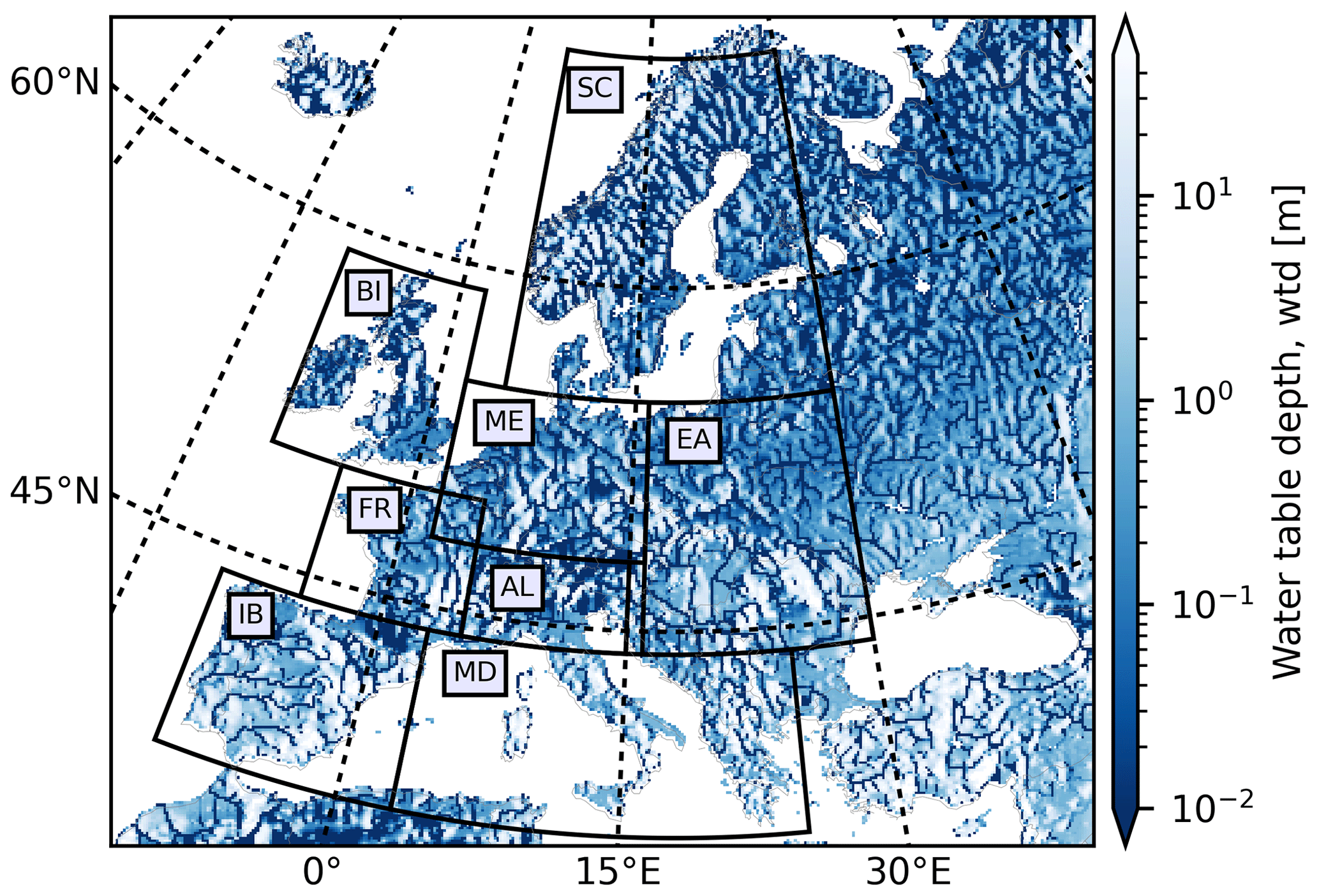
Figure 3 TSMP-G2A wtd (meters) climatology over the European continent for the time period from 1996 to 2016. Areas bounded by the thick black lines show the PRUDENCE regions (i.e., SC – Scandinavia; BI – British Isles; ME – mid-Europe; EA – Eastern Europe; FR – France; AL – Alps; IB – Iberian Peninsula; MD – Mediterranean).

Table 1 Overview of the PRUDENCE regions, including region names and abbreviations, coordinates, and climatologic information extracted from the TSMP-G2A data set (expressed as average ± standard deviation).

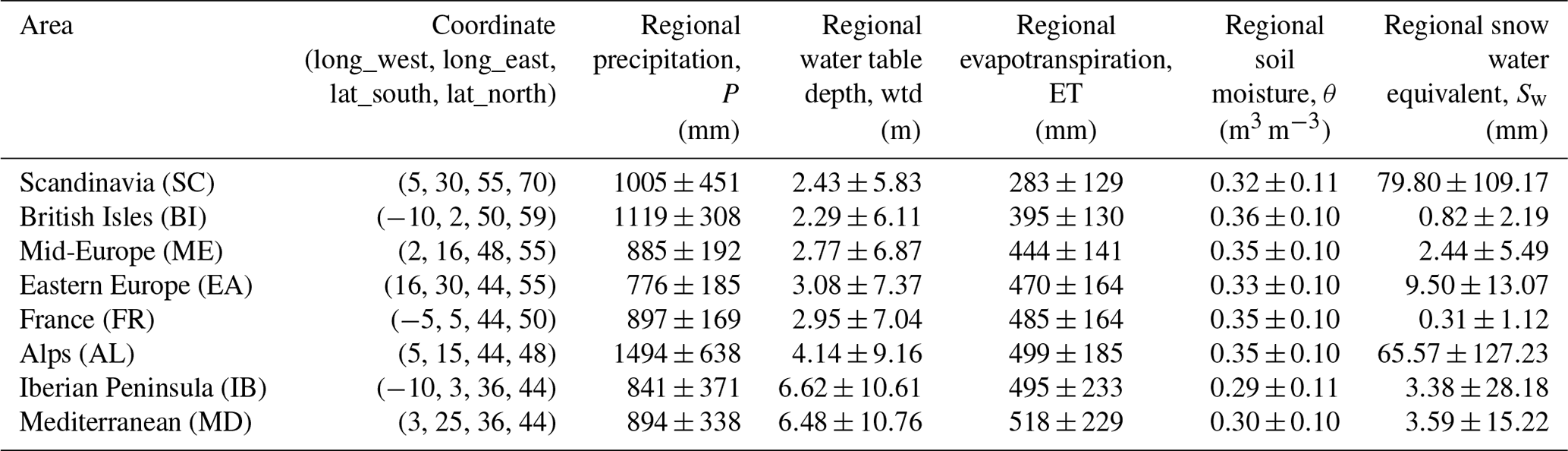
As shown by the averages in Table 1, P is heterogeneously distributed over the PRUDENCE regions, with the highest rainfall in AL (1494 mm) and the lowest in EA (776 mm). Most regional average wtd's range from 2 to 5 m, other than IB and MD (having a larger average wtd > 6 m). Within this range, AL has a relatively high average wtd (4.14 m) due to its strong relief. Higher ET is naturally observed in more arid regions, e.g., the highest regional average ET (518 mm) is recorded in MD. No significant difference is observed in regional average θ over PRUDENCE regions, and the minimal regional average θ is observed in IB (0.29 m³ m⁻³) and MD (0.30 m³ m⁻³). For S_w, large values (>60 mm) are simulated in SC and AL, while values below 10 mm are recorded in the other regions.

We utilized the TSMP-G2A data set to compute pr_a and wtd_a (Eqs. 6 and 7) at the individual pixel level over Europe, which are the input and output data of the proposed LSTM networks. The associated average and standard deviation values are based on the training set (i.e., the data within the years 1996 to 2012; described in Sect. 2.5) to guarantee that no future information leaks into the networks in the training process.

$$\begin{array}{}\text{(6)}& {\mathrm{pr}}_{\mathrm{a}}=\left({\mathrm{pr}}_{\mathrm{m}}-{\mathrm{pr}}_{\mathrm{av}}\right)/{\mathrm{pr}}_{\mathrm{sd}},\end{array}$$

where pr_m is the monthly sum P calculated from the TSMP-G2A data set, pr_av is the climatological average of pr_m (i.e., averages of pr_m in January, February, …, December), and pr_sd is the climatological standard deviation of pr_m.

$$\begin{array}{}\text{(7)}& {\mathrm{wtd}}_{\mathrm{a}}=\left({\mathrm{wtd}}_{\mathrm{m}}-{\mathrm{wtd}}_{\mathrm{av}}\right)/{\mathrm{wtd}}_{\mathrm{sd}},\end{array}$$

where wtd_m is the monthly average wtd derived from the TSMP-G2A data set, wtd_av is the climatological average of wtd_m, and wtd_sd is the climatological standard deviation of wtd_m.

The wtd_a is a measure of groundwater drought. Here we define wtd_a ≥ 2 corresponding to extreme drought, 1.5 ≤ wtd_a < 2 corresponding to severe drought, 1 ≤ wtd_a < 1.5 corresponding to moderate drought, 0 ≤ wtd_a < 1 corresponding to minor drought, and wtd_a < 0 corresponding to no drought, following McKee et al. (1993).

To identify the effect of local factors on the network behaviors, we categorized the network performances based on different intervals of yearly averaged wtd, ET, θ, S_w, and S_t and dominant PFT. The data of θ were calculated based on the information at a depth from 0 to 5 cm below the land surface. It is important to note that the data used in this study cover the years 1996 to 2016 (except for S_w data, which are only available from 2003 to 2010) to ensure that spinup effects do not impact the analyses (Furusho-Percot et al., 2019).

2.5 Experiment design

LSTM networks are employed here to detect connections between pr_a and wtd_a from the pan-European simulation results and utilize pr_a as input to predict wtd_a. At each time step, one new input enters a network, together with information stored in the network's memory (i.e., useful messages from inputs in the past) to generate outputs. Therefore, LSTM networks have the ability to handle the lagged response of wtd_a to pr_a.

Table 2 Hyperparameter settings of the proposed LSTM networks.

^* U (−0.5, 0.5) – uniform distribution bounded by −0.5 and 0.5.

Monthly anomaly time series at individual pixels were divided into three parts for network training (January 1996–December 2012), validation (January 2013–December 2014), and testing (January 2015–December 2016) containing about 80 %, 10 %, and 10 % of the total data, respectively. In training, the network is fitted to a given training set by adjusting its weights and biases. The technique of adjusting network parameters is called an optimizer that minimizes a cost function at a certain learning rate (Govindaraju, 2000). This study utilized a supervised training algorithm with a supplementary teacher signal (i.e., TSMP-G2A monthly wtd_a) to guide the training process, which is widely adopted in hydroscience in case of, e.g., stream stage modeling (Sung et al., 2017), stream discharge modeling (Zhang et al., 2015), and groundwater level modeling (Adamowski and Chan, 2011). One common challenge in the training process is overfitting. Validation is a process to address overfitting by comparing the network output with the teacher signal to obtain a validation loss (Govindaraju, 2000; Liong et al., 2000). Provided that the network has gained sufficient knowledge from the training set, training ceases when the number of epochs (i.e., an iteration when the whole training set travels through the network forward and backward once) is ≥50, and the validation loss starts increasing. The strategy to stop training based on validation losses is termed early stopping.

Moreover, the validation losses were applied to tune hyperparameters of the LSTM networks whose architecture was introduced in Sect. 2.2. To simplify the procedure of hyperparameter tuning, we only focused on the optimization of the number of hidden neurons in this study and set other hyperparameters to be constant (Table 2). The networks with hidden neurons from 1 to 100 were trained at individual pixels, and the best three of them were selected for testing based on the validation losses.

Finally, during testing, the optimally trained networks were provided with a previously unknown data set, originating from the same source as the training set. The difference between generated and target values during testing is called the generalization error, representing the ability of a network to perform on previously unobserved data. The average of the three optimal network results was utilized for evaluation in order to moderately eliminate the individual deficiencies of the selected networks, thereby improving the quality of the final results (Goodfellow et al., 2017; Brownlee, 2018). The metrics to assess network performance in this study are the root mean square error (RMSE), the coefficient of determination (R²), and the bias from R (α), as shown in Eqs. (8)–(10), respectively. α indicates systematic additive and multiplicative biases in the generated values, with a value between 0 and 1, where α=1 means no bias (Duveiller et al., 2016).

$$\begin{array}{}\text{(8)}& {\displaystyle }\mathrm{RMSE}=\sqrt{\sum _{i=\mathrm{1}}^N{\left(y_{\exp }-y_{\mathrm{gene}}\right)}^{\mathrm{2}}/N},\text{(9)}& {\displaystyle }{R}^{\mathrm{2}}=\mathrm{1}-\sum _{i=\mathrm{1}}^N{\left(y_{\exp }-y_{\mathrm{gene}}\right)}^{\mathrm{2}}/\sum _{i=\mathrm{1}}^N{\left(y_{\exp }-\stackrel{\mathrm{‾}}{y_{\exp }}\right)}^{\mathrm{2}},\text{(10)}& {\displaystyle }\begin{array}{rl}\mathit{\alpha }=& \mathrm{2}/\left[{\mathit{\sigma }}_{y_{\exp }}/{\mathit{\sigma }}_{y_{\mathrm{gene}}}+{\mathit{\sigma }}_{y_{\mathrm{gene}}}/{\mathit{\sigma }}_{y_{\exp }}+{\left(\stackrel{\mathrm{‾}}{y_{\exp }}-\stackrel{\mathrm{‾}}{y_{\mathrm{gene}}}\right)}^{\mathrm{2}}/\right.\\ & \left.\left({\mathit{\sigma }}_{y_{\exp }}{\mathit{\sigma }}_{y_{\mathrm{gene}}}\right)\right]\end{array},\end{array}$$

where y_exp, $\stackrel{\mathrm{‾}}{y_{\exp }}$, and ${\mathit{\sigma }}_{y_{\exp }}$ are the expected value, the average of the expected values, and the standard deviation of the expected values, respectively. y_gene, $\stackrel{\mathrm{‾}}{y_{\mathrm{gene}}}$, and ${\mathit{\sigma }}_{y_{\mathrm{gene}}}$ are the generated value, the average of the generated values, and the standard deviation of the generated values, respectively. N is the number of time steps in the given time series.

Repeating the above network training, validation, and testing processes (right panel of Fig. 4), we constructed the proposed LSTM networks locally at ≤200 px randomly selected in each group in order to save computing time. As described in Sect. 2.4, climatologic differences occur not only between different PRUDENCE regions but also at certain pixels in the same region, which potentially explains varying network performances at individual pixels. To analyze the network reaction to local factors, we categorized the pixels into groups based on various intervals of yearly averaged wtd, ET, θ, S_w, and S_t and dominant PFT (Table 3), and the analysis results will be presented in Sect. 3.2. Figure 4 gives a generic workflow of this study to establish the LSTM networks at the local scale and analyze their output.

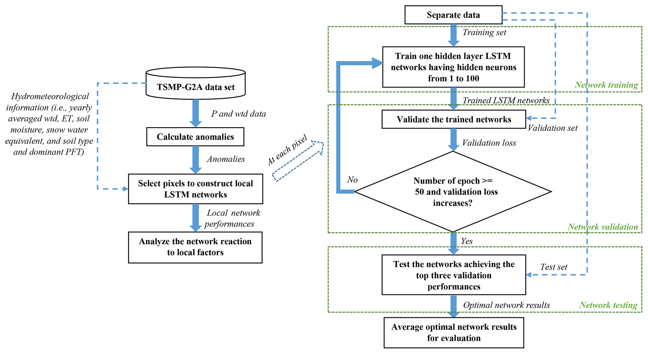
Figure 4 Workflow for LSTM network setup over the European CORDEX domain. The left section represents the overall processes of the network setup, whereas the right section shows how to apply LSTM networks at a selected pixel. The blue dashed lines with arrows indicate additional data transmission paths.

Table 3 Intervals of yearly averaged wtd, ET, θ, S_w, and S_t and dominant PFT for categorization.

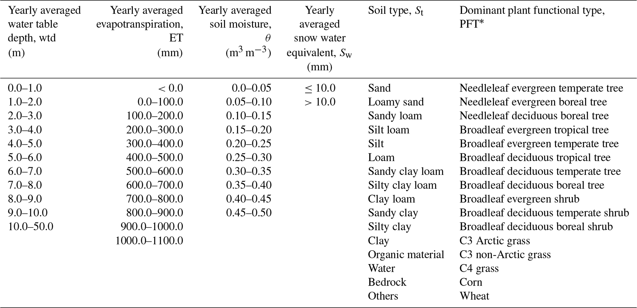
^* Dominant PFT – the PFT of which the percentage is ≥50 % at 1 px.

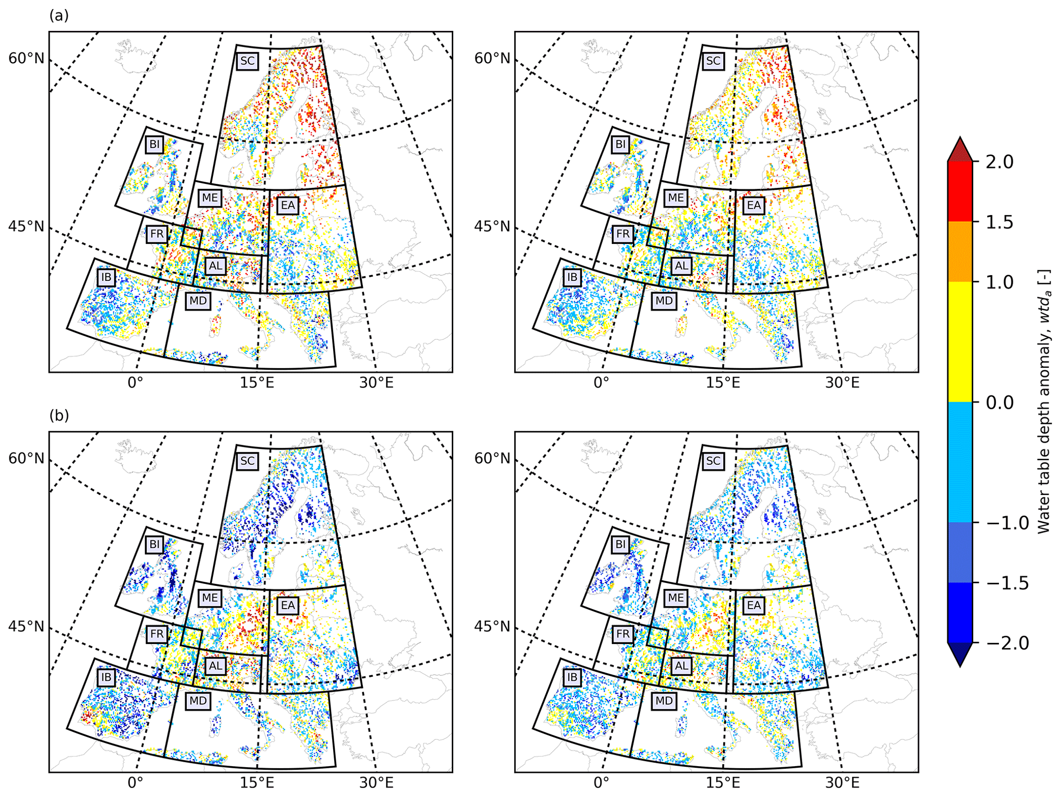
Figure 5 European wtd_a maps for (a) August 2003 (i.e., in the training period) and (b) August 2015 (i.e., in the testing period) derived from the TSMP-G2A data set (left) and the results from LSTM networks (right).

3 Results and discussion

3.1 Water table depth anomaly maps in 2003 and 2015 reproduced by the LSTM network results

We employed the outputs of the proposed LSTM networks to reproduce wtd_a over the European continent in 2003 and 2015, constituting drought years (Van Loon et al., 2017). Here, we displayed the wtd_a from the TSMP-G2A data set and the networks (hereafter called LSTM wtd_a) for August 2003 (in the training period; Fig. 5a) and August 2015 (in the testing period; Fig. 5b) with respect to strength. We focused on areas where wtd_a ≥ 1.5 (i.e., a strong drought) and studied the consistency between the TSMP-G2A and the LSTM wtd_a results on the distribution of groundwater drought. As the LSTM networks performed well at most pixels during the training period, the LSTM wtd_a map appears almost identical to the TSMP-G2A wtd_a map for August 2003 (see Fig. 5a), showing severe groundwater drought in most parts of Europe, which is in good agreement with previous studies (Andersen et al., 2005; Van Loon et al., 2017). Moreover, in the simulations and LSTM results, there is increased groundwater storage over central Germany, central Britain, southeastern France, the western Iberian Peninsula, and several parts of Eastern Europe, illustrating the strong spatial heterogeneity of the anomalies, which is expected. In contrast, due to decreased network performance during testing, the LSTM wtd_a map shows less agreement with the TSMP-G2A wtd_a map for August 2015 (see Fig. 5b) with respect to the severity of drought. Extremes in wet and dry anomalies (i.e., |wtd_a| ≥ 2) were especially underestimated, suggesting that the training set contains too little information on extreme events and, thus, is too short. Yet overall, a visual inspection of Fig. 5b shows that the LSTM wtd_a map agrees well with the TSMP-G2A wtd_a map on the spatial distribution of dry and wet events. In both maps, we identified severe drought in mid-Europe, the Alps, and the northwest of Eastern Europe, lending confidence in the trained networks to predict wtd_a from pr_a information. Additional European wtd_a maps for the second half of 2003 and 2015 are shown in Appendix B, leading to similar conclusions regarding the ability of the LSTM results to reproduce TSMP-G2A wtd_a.

3.2 Impact of local factors on the network performance

In each PRUDENCE region, we computed the averages and standard deviations of the test R² scores and RMSEs for the categories based on different intervals (Table 3) of yearly averaged wtd, ET, θ, S_w, and S_t and dominant PFT (Fig. 6) to study dependents of the network test performances on different local factors. For statistical significance, we only considered categories with ≥50 px. In addition, negative R² values at the pixel level were set to zero in the calculation of averages and standard deviations.

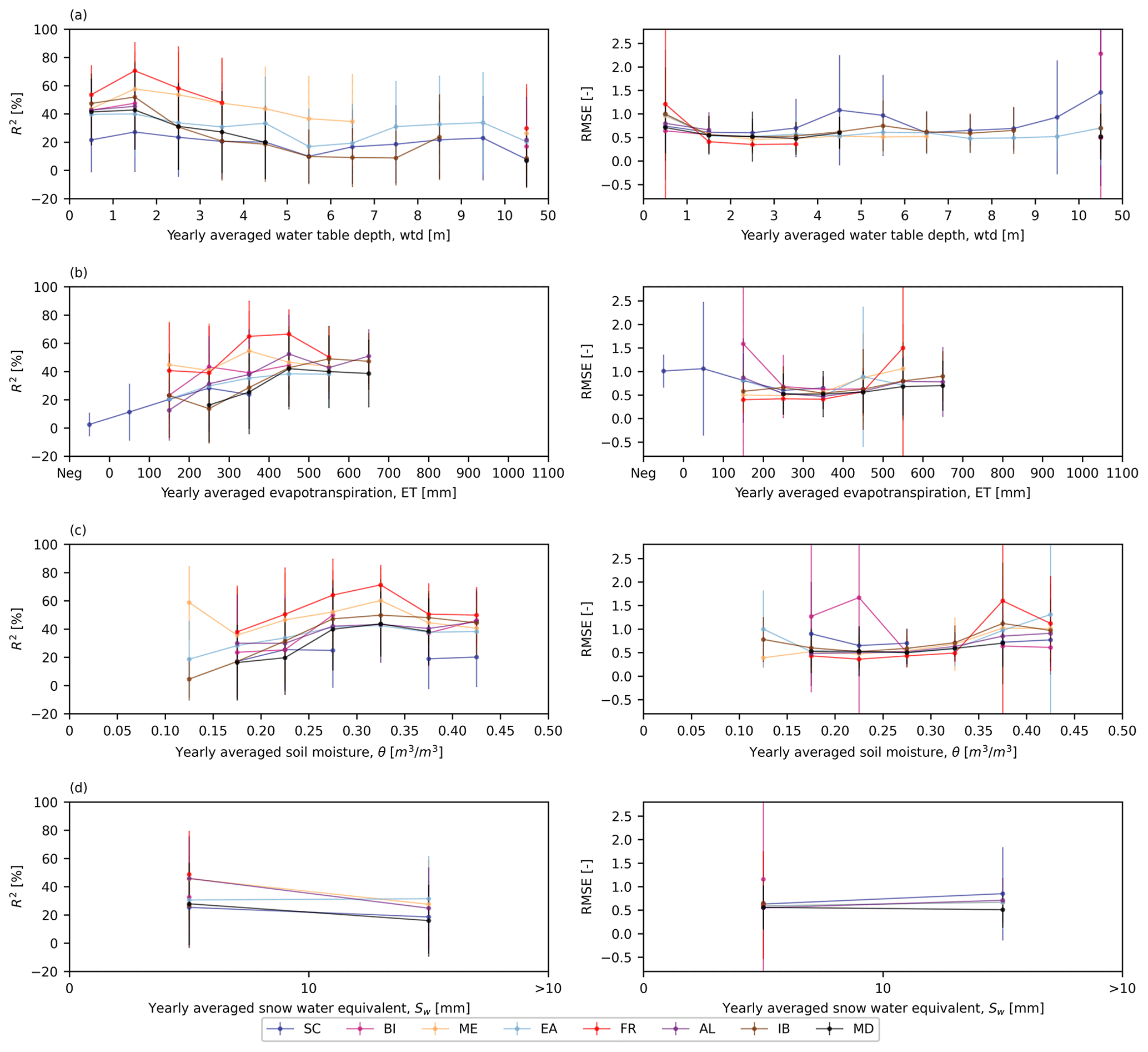
Figure 6 Averages and standard deviations of the test R² scores (left) and RMSEs (right) over the categorized results. Shown are the yearly averaged (a) wtd, (b) ET, (c) θ, and (d) S_w. The averages are indicated as dots, while the bars indicate standard deviations. The different colors reflect test results in different PRUDENCE regions.

There was no significant influence of S_t and dominant PFT on the scores (not shown here). In general, the performance decreased with increasing yearly averaged wtd, which was manifested by decreasing average R² scores and growing average RMSEs (Fig. 6a). This type of network behavior can be attributed to a stronger connection of groundwater to P in shallow aquifers, which is intuitive. In contrast to the impact of yearly averaged wtd on the test performance, the performance was positively correlated to yearly averaged ET and θ. With increasing yearly averaged ET (Fig. 6b) or θ (Fig. 6c), there was an increase in average R² scores and a decrease in average RMSEs. We can explain this phenomenon by the overlap between low-wtd and high-ET (or high-θ) areas over Europe. We also discovered that yearly averaged S_w played an important role in the network test performance. In most PRUDENCE regions, the performance decreased in the case of increasing S_w, leading to smaller average R² scores and larger average RMSEs presented in Fig. 6d. The reason is that snow accumulation resulted in complex feedback with groundwater processes that cannot be captured well by the networks without including additional input information. Overall, in the same region, most of the proposed LSTM networks achieved a relatively good test performance at the pixels with yearly averaged wtd <3 m, ET > 200 mm, θ>0.15 m³ m⁻³ and S_w<10 mm, where a stronger relationship exists between pr_a and wtd_a.

As mentioned in Sect. 2.4, we only used the training set to calculate the climatological average and standard deviation in order to prevent the networks from incorporating future information in the training process. However, some extreme values in the validation and test sets may exceed the range of the training set, resulting in decreased validation and test performances and suggesting that a varying pattern may exist between pr_a and wtd_a over the study period (see discussion in Sect. 3.3). This can also be a potential reason for large standard deviations in the test RMSEs in Fig. 6.

Figure 6 also reveals different regional network test performances. In the same interval of yearly averaged wtd, the difference in yearly average R² scores between two PRUDENCE regions can be more than 40 %. FR exhibits the overall best network performance during testing. As shown in Table 1, the regional average wtd, ET, θ, and S_w of FR are 2.95 m (<3 m), 485 mm (>200 mm), 0.35 m³ m⁻³ (>0.15 m³ m⁻³), and 0.31 mm (<10 mm), respectively. Hence, there was a close connection between pr_a and wtd_a at most pixels in FR, resulting in good network test performance.

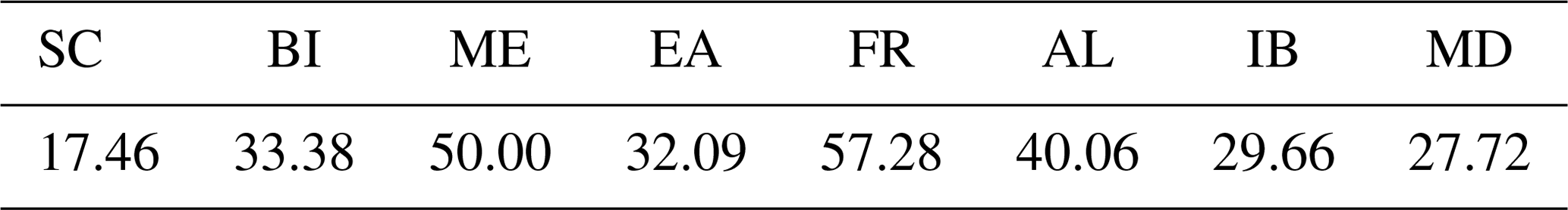
To further analyze the network test performances in different PRUDENCE regions, Fig. 7 and Table 4 provide test R² scores over Europe and percentages of the selected pixels with test R²≥50 %, respectively. FR outperformed the other regions on test R² scores, which is consistent with the finding from Fig. 6. In BI, ME, EA, and AL, the proposed LSTM networks behaved well during testing (i.e., having test R²≥50 %) at more than 30 % of the selected pixels (colored in blue in Fig. 7). However, we also found low percentages of the selected pixels with test R²≥50 % in SC, IB, and MD, which are 17.46 %, 29.66 %, and 27.72 %, respectively. In Table 1, SC is characterized as the region with the largest regional average S_w (79.80 mm) and the smallest regional average ET (283 mm), and as shown in Fig. 6, the networks tended to perform poorly during testing in the areas with large S_w and small ET. The pixels in IB and MD (regional average wtd > 6 m) generally have larger wtd than the other regions, resulting in a more lagged and weaker connection between pr_a and wtd_a, which is intuitive. Therefore, the network behavior in IB and MD was relatively poor.

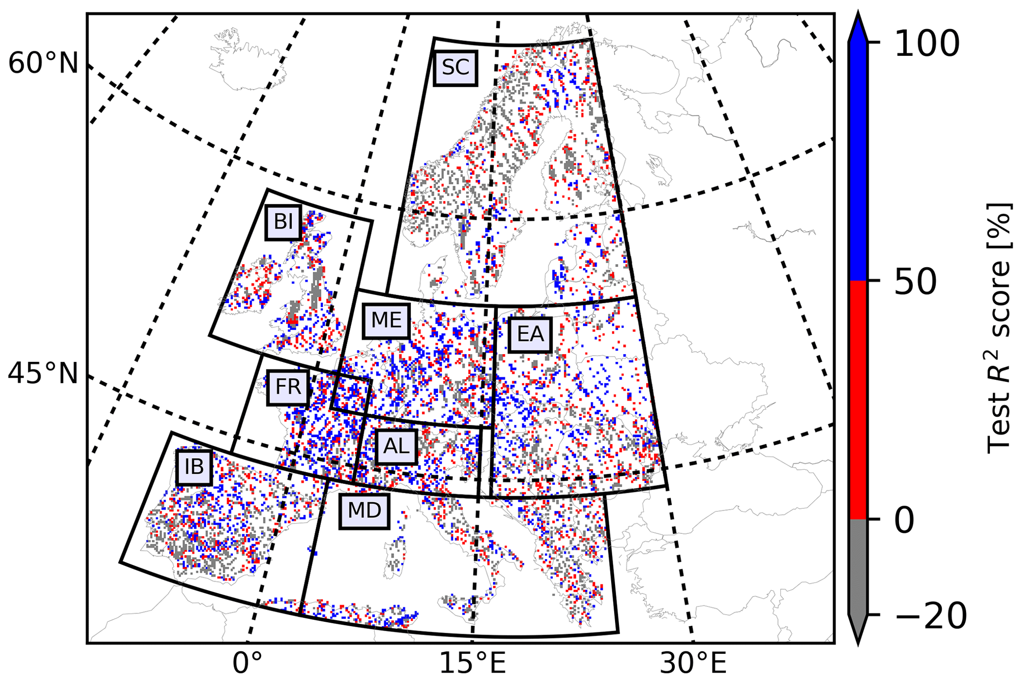
Figure 7 Map of test R² scores achieved by the proposed LSTM networks in the PRUDENCE regions.

Table 4 Percentages of the selected pixels with a test R² score ≥ 50 % in the PRUDENCE regions (percent).

We extended the scope of the analyses to the entire study period and found that the performance of individual networks generally followed two combinations with respect to training and test scores, which are as follows:

• C1 – training R² score ≥ 50 %; test R² score ≥ 50 %

• C2 – training R² score ≥ 50 %; test R² score ≤ 0 %.

The data distribution in the training and test sets was expected to be analogous, and if the networks did not encounter overfitting during training, their test performance increased by the improvement of the training performance and vice versa. C1 is the expected network behavior with both satisfactory training and test scores. C2 is an exception in which the networks that performed well on the training set failed to handle the test set. Significantly reduced test performance in C2 can be attributed to the hypothesis that the pattern between pr_a and wtd_a varied over the study period.

Figure 8 shows the percentages of the pixels where the network performance followed C1 (Fig. 8a) and C2 (Fig. 8b) in different PRUDENCE regions and intervals of wtd, ET, θ, and S_w. For statistical significance, only the regions and the intervals of wtd, ET, θ, and S_w with ≥50 selected pixels were considered. Here, we focused on the regions and the intervals with high percentages (>30 %; above the black dashed lines in Fig. 8) to identify common hydrometeorological characteristics of a pixel where the network performance followed C1 or C2. For C1, high percentages were found in regions except for SC, IB, and MD and in areas with wtd ≤ 3 m, ET ≥ 200 mm, θ≤0.10 m³ m⁻³ and θ≥0.20 m³ m⁻³, and S_w≤10 mm, which are in good agreement with our previous findings. In contrast, for C2, the percentages are high in SC, EA, IB, and MD and in areas with wtd ≥2 m, ET ≤ 300 mm, and 0.10 m³ m⁻³ < θ≤0.25 m³ m⁻³. The distribution of C2 is not very sensitive to S_w, and the percentages are large in both areas, with S_w≤10 mm and S_w>10 mm. Moreover, in areas with negative ET, there is no pixel where the network performances followed C1, and C2 is the dominant network performance combination. We explain negative ET by pronounced freezing and sublimation processes in these areas, which significantly affect the response of wtd_a to pr_a.

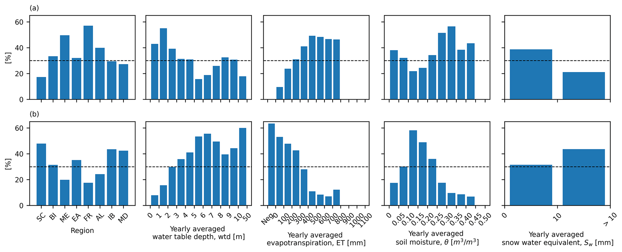
Figure 8 Bar plots showing the percentages of pixels where the network performance followed the combinations (a) C1, (b) C2 in different regions and intervals of yearly averaged wtd, ET, θ, and S_w, from left to right, respectively. Black dashed lines indicate percentages equal to 30 %.

3.3 Cross-wavelet transform (XWT) analysis

In the previous section, we posed the hypothesis that the temporal pattern between pr_a and wtd_a during training, validation, and testing was different at a number of pixels over the European continent. XWT was employed here for hypothesis testing at the individual, representative pixels (Table 5), which were randomly selected based on the hydrometeorological characteristics of C1 and C2 summarized in Fig. 8. XWT showed the time–frequency pattern in the pr_a and wtd_a time series derived from the TSMP-G2A data set (i.e., TSMP-G2A pr_a and wtd_a) at these pixels and highlighted the common high power of the frequency components in the time series (Fig. 9). The α values (Eq. 10) of pixel 1 were generally suggesting that smaller biases existed in the results of the LSTM networks. In addition, we found different α values for pixel 2, with small biases in the training and large biases in the validation and testing.

Table 5 Pixel characteristics in the XWT analysis (pixels 1–2).

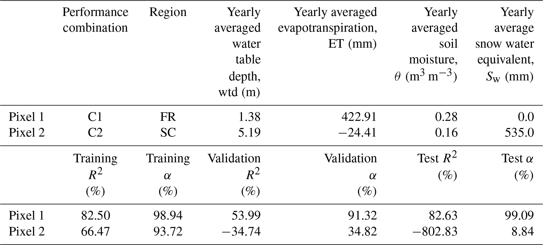
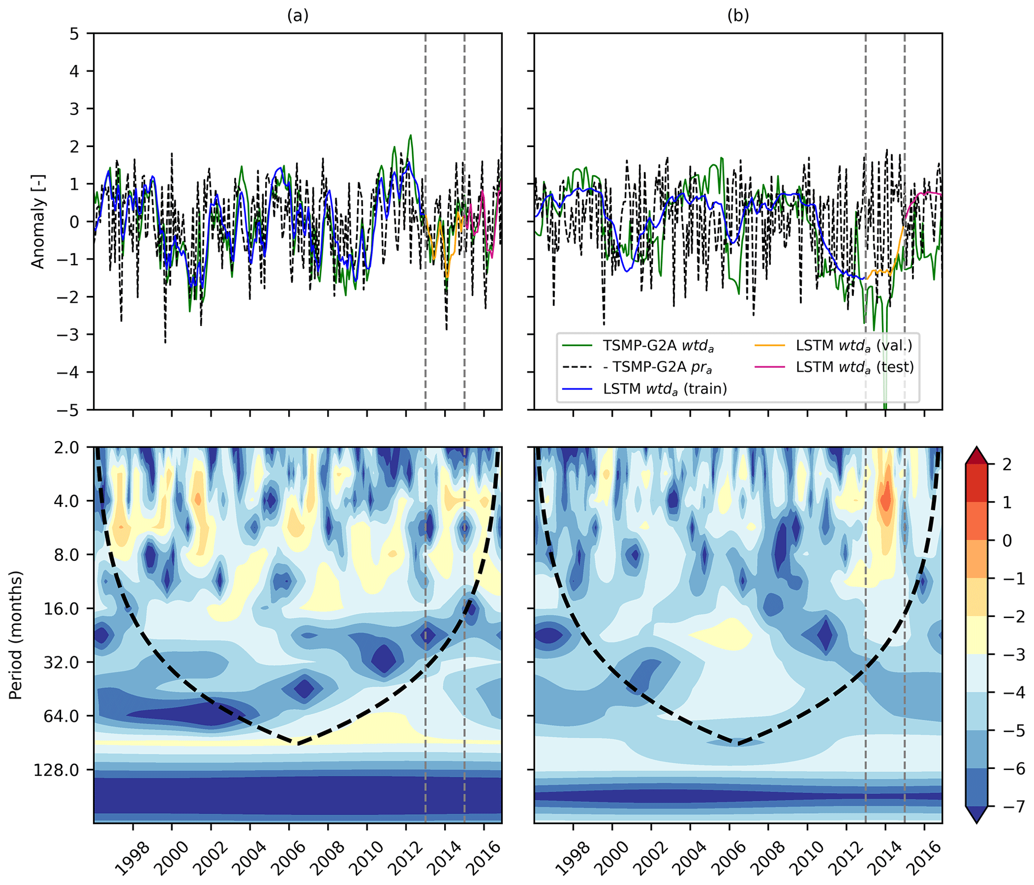
Figure 9 TSMP-G2A pr_a, TSMP-G2A wtd_a, and LSTM wtd_a time series (top), as well as cross-wavelet spectra for TSMP-G2A pr_a and wtd_a series (bottom), at a representative pixel of the performance combination (a) C1 and (b) C2. In the cross-wavelet spectra, the black dashed line marks the boundary of the cone of influence. The color bar presents log ₂(power/scale). In all plots, the two gray dashed lines separate the study period into the training, validation, and testing periods.

Figure 9 shows the results of the XWT analyses of the selected pixels in combination with the corresponding TSMP-G2A pr_a and wtd_a time series. Inspecting the results of the XWT analyses (bottom panel of Fig. 9), the concentration period of power was inconsistent in the area without edge effects (i.e., the area within the black dashed line) at pixel 2 from the time period 1996 to 2016, indicating a time-varying pattern between pr_a and wtd_a at the pixel, thus supporting our hypothesis. It also explores the high sensitivity of LSTM networks to outliers, which is a drawback of data-driven models.

The high power in the XWT results at the representative pixel of C1 (pixel 1; Fig. 9a) was consistently located in a certain period (i.e., below 64 months), indicating a consistent pattern between pr_a and wtd_a throughout the whole study period, which is the prerequisite of good network performances. At the pixel, we found that most of the high power in the XWT results was consistently concentrated in the period from 2 to 16 months during the study period (see Fig. 9a). The plot in Appendix C (Fig. C1a) showed similar phenomena as above. Therefore, we speculate that LSTM networks might be frequency aware and work well to capture the pr_a–wtd_a relationship at the monthly, seasonal, and annual periods.

4 Summary and conclusions

In this study, we proposed LSTM networks as an indirect method to model monthly wtd_a over the European continent, using monthly pr_a as input. Local LSTM networks were constructed at individual pixels randomly selected over Europe to capture the time-varying and time-lagged relationship between pr_a and wtd_a from integrated hydrologic simulation (TSMP-G2A) results covering the 1996 to 2016 episode. The monthly anomaly series derived from the TSMP-G2A data set were divided into three sections at each pixel for network training, validation, and testing. Using the output of the LSTM networks, we successfully reproduced TSMP-G2A wtd_a maps over Europe for drought months in both the training and testing period (e.g., August 2003 and August 2015) in terms of the spatial distribution of dry and wet events. The good agreement between the TSMP-G2A and LSTM wtd_a maps demonstrated the ability of the trained networks to model wtd_a from pr_a data. The results highlighted the impact of local factors on the network test performance, as manifested by R² scores and RMSEs. Most of the networks attained high test R² scores at the pixels with wtd < 3 m, ET > 200 mm, θ>0.15 m³ m⁻³, and S_w<10 mm, where a stronger connection existed between pr_a and wtd_a. Also, the various hydrometeorological characteristics in each PRUDENCE region resulted in regional differences in the test performance of the proposed networks, with FR showing the overall best network performance. In some regions, test performance deteriorated due to changing temporal patterns in the pr_a–wtd_a relationship, approved by XWT analyses. According to the results of the XWT analyses, we hypothesize that LSTM networks have frequency awareness and tend to perform well to capture the pr_a–wtd_a relationship at the monthly, seasonal, and annual periods.

We also recognized that the limited amount of data in the training introduces uncertainties in the network performances. Any potential extension of training data may lead to a significant improvement in the quality of the derived networks. In addition, hyperparameters of the proposed LSTM networks may be further tuned at the individual pixel level to improve network performance. Due to a lack of spatiotemporally continuous wtd observations over Europe, this study presents a methodology for deriving a LSTM network model for wtd_a from pr_a based on simulation results from a terrestrial model (i.e., the TSMP-G2A data set). As demonstrated in Furusho-Percot et al. (2019) and Hartick et al. (2021), the TSMP-G2A data set shows a good agreement with hydrometeorological and GRACE observations in different European regions. Therefore, we argue that the TSMP-G2A data set is a good reference data set to establish the methodology. The results suggest that LSTM networks are useful for estimating wtd_a time series based on other hydrometeorological variables which are routinely measured and, therefore, are more easily available from, e.g., atmospheric reanalyses and forecast data sets and observations than groundwater level measurements. After training, LSTM networks could provide fast and reliable predictions of wtd_a only based on the data of input variables, which is impossible for traditional, physically based models such as TSMP. The proposed methodology may be transferred into a real-time monitoring and forecasting workflow for wtd_a at the continental scale.

Appendix A: Pseudocode of the LSTM network (displayed in Fig. 2)

The pseudocode, shown below, is of the one hidden layer LSTM networks illustrated in Fig. 2, which is modified from Gers et al. (2000). Variables were defined in the caption of Fig. 2. Note that, in order to simplify the code, the biases are not shown here.

Appendix B: Additional European water table depth anomaly maps

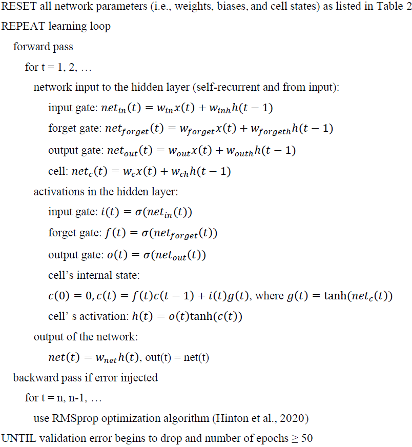
Figure B1 European wtd_a maps for (a) July 2003 (i.e., in the training period) and (b) July 2015 (i.e., in the testing period) derived from the TSMP-G2A data set (left) and the results from LSTM networks (right).

Figure B2 European wtd_a maps for (a) December 2003 (i.e., in the training period) and (b) December 2015 (i.e., in the testing period) derived from the TSMP-G2A data set (left) and the results from LSTM networks (right).

Appendix C: Results of the cross-wavelet transform (XWT) analysis at additional pixels

Table C1 Pixel characteristics in the XWT analysis (pixels 3–4).

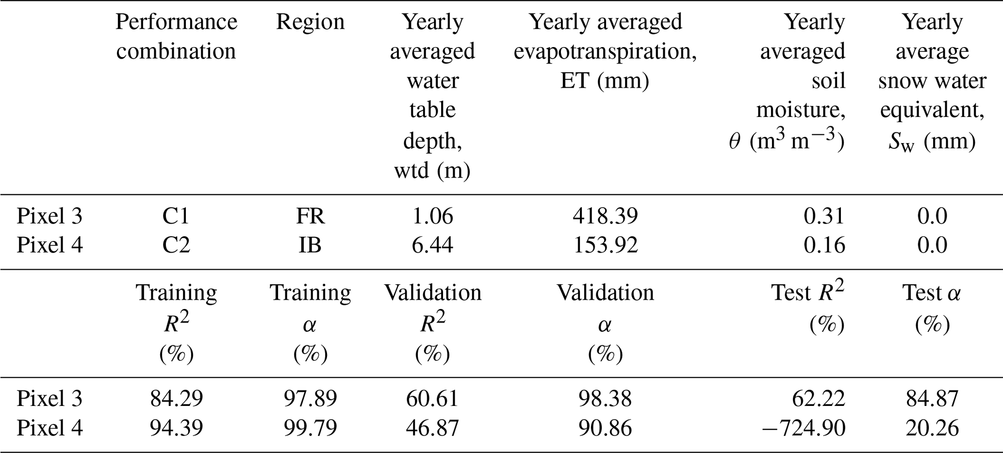
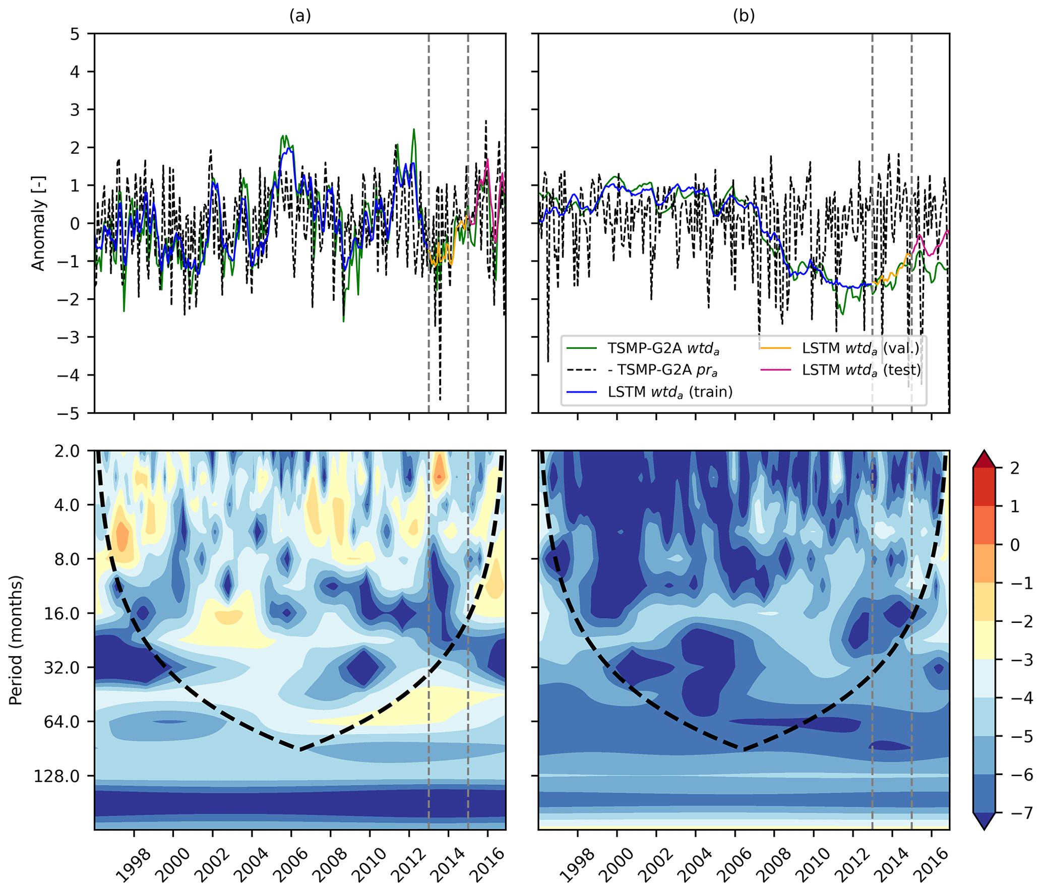
Figure C1 TSMP-G2A pr_a, TSMP-G2A wtd_a, and LSTM wtd_a time series (top), as well as cross-wavelet spectra for TSMP-G2A pr_a and wtd_a series (bottom), at (a) pixel 3 and (b) pixel 4. The lines have the same definitions as in Fig. 9.