Technical Note: Sequential ensemble data assimilation in convergent and divergent systems

Data assimilation methods are used throughout the geosciences to combine information from uncertain models and uncertain measurement data. However, the characteristics of geophysical systems differ and may be distinguished between divergent and convergent systems. In divergent systems initially nearby states will drift apart, while they will coalesce in convergent systems. This difference has implications for the application of sequential ensemble data assimilation methods. This study explores these implications on two exemplary systems, i.e., the divergent Lorenz 96 model and the convergent description of soil water movement by the Richards equation. The results show that sequential ensemble data assimilation methods require a sufficient divergent component. This makes the transfer of the methods from divergent to convergent systems challenging. We demonstrate, through a set of case studies, that it is imperative to represent model errors adequately and incorporate parameter uncertainties in ensemble data assimilation in convergent systems.

1 Introduction

Information on physical systems is often available in two forms; on the one hand, it is available from observations and on the other hand through mathematical models describing the system's dynamics. The combination of both can lead to an improved description of the system. This is the aim of data assimilation, typically with a focus on state estimation.

Data assimilation has broad applications throughout the geosciences and can be already seen as an independent discipline (Carrassi et al., 2018). It is typically used to estimate states but is also used for parameters, i.e., in weather forecasting (Houtekamer and Zhang, 2016; Ruiz et al., 2013), for atmospheric chemical transport (Carmichael et al., 2008; Zhang et al., 2012) also coupled to meteorology (Bocquet et al., 2015), in oceanography, including biogeochemical processes (Stammer et al., 2016; Edwards et al., 2015), and in hydrology for flow, transport, and reaction in terrestrial surface and subsurface systems (Liu et al., 2012). Data assimilation is also increasingly applied in ecology, with applications ranging from the spread of infectious diseases and wildfires to population dynamics and the terrestrial carbon cycle (Niu et al., 2014; Luo et al., 2011).

In this study, we distinguish between geophysical systems that are divergent or convergent systems, depending on the development of two initial nearby states (Fig. 1). In a divergent system, initially close states will inevitably drift apart, even if the system is described by a perfect model (Kalnay, 2003). This leads to an upper limit for the predictability in divergent systems (Lorenz, 1982). In a convergent system, nearby trajectories will coalesce. If the model to describe such a convergent system is perfect, this results in a high predictability (Lorenz, 1996). An error in the initial state will decay towards the truth after some transient phase. However, this is only true for perfect models, which is usually not the case for geophysical systems. This can lead to a bias with convergence to a wrong state.

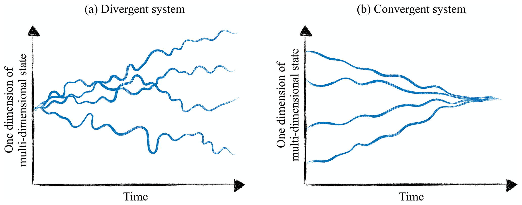
Figure 1 Dynamics of a generic divergent and convergent dynamic system with different initial states. Both panels show a single state dimension of a multi-dimensional system. In the divergent system, initially infinitesimally close states drift apart, while in the convergent system initially separate states converge.

Many recent advances in data assimilation methods have been developed in the context of weather forecasting (van Leeuwen et al., 2015). They are, therefore, designed to meet the challenges in the atmosphere – a predominantly divergent system. Due to the fundamental limit for long time predictions from uncertain initial conditions in divergent systems, data assimilation in operational weather forecasting primarily focuses on state estimation (Reichle, 2008; van Leeuwen et al., 2015).

While weather forecasting or oceanography are divergent systems, several geophysical systems, such as soil hydrology or chemical transport, are convergent systems. In ensemble data assimilation methods, if uncertainties are only represented through an ensemble of states, convergent systems lead to decreasing uncertainties over time, which favors filter degeneration. This difference to divergent systems, where the ensemble spread increases exponentially, makes the direct transfer of data assimilation methods from divergent systems to convergent systems challenging and often requires adaptations to prevent filter degeneracy. The application of data assimilation when coupling a divergent and a convergent model, for example, in coupled chemistry meteorology models, may potentially lead to new difficulties (Bocquet et al., 2015).

The largest uncertainties in convergent systems typically do not reside in uncertain initial conditions but rather in boundary conditions, which include external forcings, the representation of sub-scale physics through parameterizations, and unrepresented physics in the model equations. These uncertainties should then be addressed in an integrated manner (Liu and Gupta, 2007). Therefore, data assimilation methods have been used to not only estimate states but also parameters to reduce these uncertainties. The combined estimation of states and parameters is thought to be a solution for reducing the impact of model errors on parameter estimation (Liu et al., 2012). Estimating parameters in ensemble data assimilation methods through an augmented state requires a forward model for the parameters as well. This model is typically assumed to be constant, which is neither divergent nor convergent. However, the filter will gradually reduce the uncertainty in the parameters, which is not increased through a divergent forward model, and challenges similar to convergent systems can arise. This is sometimes alleviated by assigning a random walk as the forward model to the parameters, which then requires to determine an appropriate step size.

A challenge for sequential ensemble data assimilation in convergent systems is to maintain a sufficient ensemble spread. This would require an adequate representation of all uncertainties, including unrepresented physics in the model equations. In real-world systems, this is often difficult or impossible. Therefore, practical alternatives are necessary, which are often heuristic and may interfere with basic assumptions in the data assimilation methods. One possibility is inflation methods, which counteract the coalescing tendency. Unfortunately, there exists no universal method to accomplish this, and a range of approaches are followed. One example is the increase in the ensemble spread of parameters to a threshold value, as soon as the parameter uncertainty drops below this value. This approach was introduced for a sea breeze model (Aksoy et al., 2006) and has been used in hydrology as well (e.g., Shi et al., 2014; Rasmussen et al., 2015). A modification to this, also applied in hydrology, is to keep the parameter uncertainty entirely constant (Han et al., 2014; Zhang et al., 2017). This ensures a sufficient ensemble spread in the state itself but can impact the accuracy of the estimation. A widely used adjustment to limit the reduction in an ensemble spread in hydrology is the use of a damping factor (Hendricks Franssen and Kinzelbach, 2008). In soil hydrology, a multiplicative inflation method was proposed and specifically adjusted to the needs of the system (Bauser et al., 2018). Similarly, Constantinescu et al. (2007) showed that an atmospheric chemical transport model required much stronger inflation than reported in the meteorological literature and showed better results for a model-specific inflation, where the key parameters are perturbed to achieve an increased spread in the state. Consequently, a better understanding and control over errors has been recognized as a major challenge in chemical data assimilation as well (Zhang et al., 2012).

Although plenty of knowledge and experience are available in the different communities on how to handle data assimilation methods in their specific models, we are not aware of a fundamental analysis of the difference between divergent and convergent models with respect to their utilization within ensemble data assimilation frameworks. We investigate and demonstrate the different challenges that illustrate, for example, the different requirements for inflation methods, using the ensemble Kalman filter (Evensen, 1994; Burgers et al., 1998). The divergent case is illustrated using the Lorenz 96 model (Lorenz, 1996), while for the convergent case, a soil hydrological system described by Richards' equation is used. Naturally, these are highly simplified models compared to real-world applications. Still, they demonstrate key aspects that also have to be addressed in more complicated situations. The specific adjustments applied there depend on the particular model. Our focus here is on the fundamentals and not on the wide range of specifics.

2 Data assimilation method

For this study we chose the ensemble Kalman filter (EnKF), a sequential data assimilation method, based on Bayes' theorem and the assumption of unbiased Gaussian error distributions. It was introduced as an extension of the Kalman filter (Kalman, 1960) for nonlinear models (Evensen, 1994; Burgers et al., 1998) and approximates the Gaussian distributions by an ensemble of states ψ_i, where the subscript i denotes the ensemble member.

To sequentially assimilate new observations, the EnKF alternates between a forecast (subscript “f”) and an analysis step (subscript “a”). In the forecast, the ensemble is propagated using the nonlinear model f(⋅) as follows:

$$\begin{array}{}\text{(1)}& {\mathit{\psi }}_{\mathrm{f},i}^k=f\left({\mathit{\psi }}_{\mathrm{f},i}^{k-\mathrm{1}}\right)+{\mathit{\beta }}^k,\end{array}$$

where β^k is a stochastic model error and k is a discrete time.

In the following, the analysis state ψ_a is calculated by applying the Kalman gain:

$$\begin{array}{}\text{(2)}& {\mathbf{K}}^k={\mathbf{P}}_{\mathrm{f}}^k{\mathbf{H}}^{\mathit{⊺}}{\left({\mathbf{HP}}_{\mathrm{f}}^k{\mathbf{H}}^{\mathit{⊺}}+{\mathbf{R}}^k\right)}^{-\mathrm{1}},\end{array}$$

to every ensemble member. The Kalman gain weights the forecast error covariance P with the observation error covariance R. The observation operator H maps the state from state space to observation space. The forecast error covariance P is calculated using the forecast ensemble as follows:

$$\begin{array}{}\text{(3)}& {\mathbf{P}}_{\mathrm{f}}^k=\stackrel{\mathrm{‾}}{\left({\mathit{\psi }}_{\mathrm{f}}^k-\stackrel{\mathrm{‾}}{{\mathit{\psi }}_{\mathrm{f}}^k}\right){\left({\mathit{\psi }}_{\mathrm{f}}^k-\stackrel{\mathrm{‾}}{{\mathit{\psi }}_{\mathrm{f}}^k}\right)}^{\mathit{⊺}}}.\end{array}$$

It is necessary to add a realization of the observation error to the observation for each ensemble member (Burgers et al., 1998). The resulting analysis state is as follows:

$$\begin{array}{}\text{(4)}& {\mathit{\psi }}_{\mathrm{a},i}^k={\mathit{\psi }}_{\mathrm{f},i}^k+{\mathbf{K}}^k\left({\mathbf{d}}^k-\mathbf{H}{\mathit{\psi }}_{\mathrm{f},i}^k+{\mathit{ϵ}}_i^k\right),{\mathit{ϵ}}_i^k\propto \mathcal{N}\left(\mathbf{0},{\mathbf{R}}^k\right).\end{array}$$

By combining the information from the measurement and the model, the uncertainty in the analysis ensemble is decreased. For sequential data assimilation, the process of forecast and analysis is iterated for every new observation.

The joint estimation of states and parameters can be realized through state augmentation. The original state ψ is extended with the parameters p to an augmented state, as follows:

$$\begin{array}{}\text{(5)}& {\displaystyle }\mathit{u}=\left(\begin{array}{c}\mathit{\psi }\\ \mathbf{p}\end{array}\right).\end{array}$$

The model equation (Eq. 1) changes to the following:

$$\begin{array}{}\text{(6)}& {\displaystyle }{\mathbf{u}}^k=\left(\begin{array}{c}{\mathit{\psi }}^k\\ {\mathbf{p}}^k\end{array}\right)=\left(\begin{array}{c}{f}_{\mathit{\psi }}\left({\mathit{\psi }}^{k-\mathrm{1}},{\mathbf{p}}^{k-\mathrm{1}}\right)+{\mathit{\beta }}_{\mathit{\psi }}^k\\ f_{\mathbf{p}}\left({\mathbf{p}}^{k-\mathrm{1}}\right)+{\mathit{\beta }}_{\mathbf{p}}\end{array}\right),\end{array}$$

with the models for the state f_ψ(⋅) and for the parameters f_p(⋅), as well as the corresponding model errors β_ψ and β_p. The model for the state is typically nonlinear, while the parameters are often assumed constant $f_{\mathbf{p}}\left({\mathbf{p}}^{k-\mathrm{1}}\right)={\mathbf{p}}^{k-\mathrm{1}}$.

In this study, we set both stochastic model errors in Eq. (6) to zero. The EnKF is used without any extensions, and an ensemble size of N=100 was chosen for all cases.

3 Divergent system

This section demonstrates the data assimilation behavior for a divergent system on the example of the 40-dimensional Lorenz 96 model, which has been widely used to test data assimilation methods in atmospheric sciences (e.g., Li et al., 2009). We first introduce the model before we look into four characteristically different cases.

3.1 Lorenz 96

The Lorenz 96 model (Lorenz, 1996) is an artificial model and cannot be derived from any dynamic equation (Lorenz, 2005). It can be interpreted as an unspecified scalar quantity x in a one-dimensional atmosphere on a latitude circle and was defined in a study on predictability (Lorenz, 1996).

The governing equations are a set of coupled ordinary differential equations as follows:

$$\begin{array}{}\text{(7)}& {\displaystyle \frac{\mathrm{d}{x}_i}{\mathrm{d}t}}=\left(x_{i+\mathrm{1}}-x_{i-\mathrm{2}}\right)x_{i-\mathrm{1}}-x_i+F,i\in [\mathrm{1},\mathrm{2},\mathrm{\dots },J],\end{array}$$

with constant forcing F, periodic boundaries ($x_{J+\mathrm{1}}=x_{\mathrm{1}}$), and dimension J. The dimension is often chosen as J=40, which we also do in this study. Even though the system is not derived from physical principles, it shares certain properties of large atmospheric models (Lorenz and Emanuel, 1998). The quadratic terms represent advection and conserve the total energy, while the linear term decreases the total energy comparable to dissipation. The constant F represents external forcing and prevents the system's total energy from decaying to zero. The value is often chosen as F=8 (Lorenz and Emanuel, 1998).

The Lyapunov exponent quantifies how fast two initially infinitesimally close trajectories will separate. Analyzing the leading Lyapunov exponent for F=8 shows a doubling time of τ_d=0.42 units for the distance between two initially infinitesimally close neighboring states (Lorenz and Emanuel, 1998). Increasing the forcing leads to a more divergent system, for instance, τ_d=0.3 for F=10 (Lorenz, 1996). With τ_d decreasing, so does the predictability of the system.

3.2 Characteristic cases

The behavior of the EnKF on a divergent system is investigated through four different cases (DC1–4), which are purposely designed in a simple manner to illustrate the behavior concisely. For all cases, the model is solved using a fourth-order Runge–Kutta method with a time step of Δt=0.01.

The initial condition for the synthetic truth for all cases is generated by running the model until time 2000 from an initial state $x_i=\mathrm{4.0}\forall i\in [\mathrm{1},\mathrm{2},\mathrm{\dots },\mathrm{39}]$ and x₄₀=4.001, with the typical value F=8 for the forcing parameter. The final state of this run is used as the synthetic true initial state for all cases. This ensures that the state is on the attractor without the initial transient phase. The initial ensemble for the data assimilation runs is generated by perturbing the true initial state with a Gaussian distribution 𝒩(0,1).

Synthetic observations are generated in all 40 dimensions by a forward run until time 4, using the true value and perturbing it with a Gaussian distribution with a zero mean and a standard deviation of σ_obs=1.0. For cases DC1 and DC2, observations are generated at eight different times with an observation interval of Δt_Obs=0.5. This observation interval is chosen to be rather large to ensure a large divergence of the system. For cases DC3 and DC4, observations are generated at 80 different times with an observation interval of Δt_Obs=0.05. This interval is often used in other studies (e.g., Nakano et al., 2007; van Leeuwen, 2010; Poterjoy, 2016).

3.2.1 Divergent case 1 (DC1) – state estimation and true parameter

In this case, the ensemble is propagated with the same parameter (F=8) as the synthetic truth. Uncertainty only stems from the uncertainty in the initial condition. Figure 2a shows the time development of one state dimension of the Lorenz 96 model (upper plot) and the ensemble variance of this state dimension ${\mathit{\sigma }}_{\dim }^{\mathrm{2}}$, together with the mean variance over all dimensions σ² (lower plot). Due to the divergent nature of the model, the ensemble spread increases between observations, and the ensemble has a sufficient spread, such that the EnKF is able to correct the states to follow the truth.

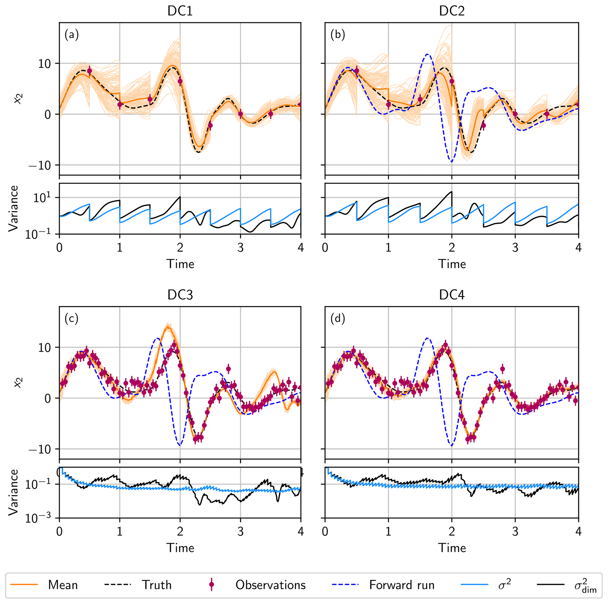
Figure 2 State estimation in a divergent system. (a) Divergent case 1 (DC1), where the ensemble is propagated with the same parameter as the truth (F=8). (b) Divergent case 2 (DC2), where the ensemble is propagated with F=10 instead. (c) Divergent case 3 (DC3), where the ensemble is propagated with F=10, and the observation interval is reduced to Δt_Obs=0.05. (d) Divergent case 4 (DC4), where the parameter error is represented by the ensemble, using 𝒩(10,2²) for the reduced observation interval of Δt_Obs=0.05. In the upper plots (a–d), the ensemble mean (orange line) and the ensemble (light orange lines) in the data assimilation run for state dimension 2 x₂, together with the observations (purple) generated from the truth (black dashed line). Panels (b–d) additionally show a single forward run (blue dashed line) using a wrong parameter F=10 starting from the true initial condition. In the lower plots (a–d), the mean variance σ² of the ensemble over all dimensions (light blue line) and variance ${\mathit{\sigma }}_{\dim }^{\mathrm{2}}$ of state dimension 2 (black line).

The mean ensemble spread σ² increases exponentially between two observations. At each observation, the EnKF updates the ensemble, and the variance decreases correspondingly.

The behavior of ${\mathit{\sigma }}_{\dim }^{\mathrm{2}}$ differs from the behavior of σ². During the forecast, ${\mathit{\sigma }}_{\dim }^{\mathrm{2}}$ sometimes increases, decreases, or stays approximately constant. This occurs because the Lorenz 96 model is bounded and has, therefore, convergent and divergent directions.

3.2.2 Divergent case 2 (DC2) – state estimation and wrong parameter

In this case, in order to investigate the impact of an unrepresented model error, the ensemble is propagated with a wrong parameter of F=10 instead of F=8 (Fig. 2b), which was used to generate the observations. Therefore, the ensemble is propagated with a model that is more divergent than the synthetic truth.

Compared to DC1 (Fig. 2a; lower plot), σ² and ${\mathit{\sigma }}_{\dim }^{\mathrm{2}}$ increase faster, and the ensemble spread reaches higher values, which shows the increased divergence of the system. Propagating the ensemble with this different model leads to a larger deviation in the ensemble mean from the truth (see Fig. 2b; upper plot) than in DC1. However, the divergent nature of the model ensures a sufficient ensemble spread so that the state can be corrected towards the truth, and the wrong parameter is compensated. This leads to a worsened, but still good, estimation of the truth without filter divergence.

3.2.3 Divergent case 3 (DC3) – state estimation, small observation interval, and wrong parameter

The case is similar to DC2, except that the observation interval is reduced to Δt_Obs=0.05. The high frequency of analysis steps, where the Kalman update reduces the variance in the ensemble, prevents the Lorenz 96 model from developing enough divergence to increase the ensemble spread sufficiently in the short time intervals in between (see Fig. 2c; lower plot). Although the ensemble is propagated with a more divergent model (F=10), the divergence is not sufficient enough to encompass the model error due to the wrong parameter, and the filter can degenerate (see Fig. 2c; upper plot). This is in contrast to DC2, where the Kalman filter can successfully estimate the state. However, the comparison with a forward run of the true initial state using the wrong parameter shows that the EnKF is able to improve the state significantly.

3.2.4 Divergent case 4 (DC4) – state estimation, small observation interval, and represented error

In divergent case 4 (DC4), the observation interval is, as in DC3, reduced to Δt_Obs=0.05. The parameter error is represented by the ensemble by assigning each ensemble member a different parameter F. The forcing parameter F is drawn from a Gaussian distribution 𝒩(10,2²), such that the true value lies within 1 standard deviation.

Representing the error increases σ² only slightly (Fig. 2d; lower plot) compared to DC3, but the minimal variance of ${\mathit{\sigma }}_{\dim }^{\mathrm{2}}$ has higher values. This increase is sufficient enough to help the filter so that it does not degenerate (Fig. 2d; upper plot). Representing the parameter error in the ensemble in the case of frequent observations can prevent filter degeneracy.

4 Convergent system

This section demonstrates the data assimilation behavior for a convergent system on the example of soil water flow. We, again, first introduce the model before we look into four characteristic cases.

4.1 Soil water flow

Water flow in an unsaturated porous medium can be described by the Richards equation as follows:

$$\begin{array}{}\text{(8)}& {\partial }_t\mathit{\theta }-\mathrm{\nabla }\cdot \left[K\left(\mathit{\theta }\right)\left[\mathrm{\nabla }{h}_{\mathrm{m}}\left(\mathit{\theta }\right)-\mathrm{1}\right]\right]=\mathrm{0},\end{array}$$

where θ (–) is the volumetric water content, K (L T⁻¹) is the isotropic hydraulic conductivity, and h_m (L) is the matric head.

To close Eq. (8), soil hydraulic material properties, which specify the dependency of the matric head and the hydraulic conductivity on the water content, are necessary. We use the Mualem–van Genuchten parameterization (Mualem, 1976; Van Genuchten, 1980) in its simplified form, as follows:

$$\begin{array}{}\text{(9)}& {\displaystyle }& {\displaystyle }K\left(\mathrm{\Theta }\right)=K_{\mathrm{w}}{\mathrm{\Theta }}^{\mathit{\tau }}{\left[\mathrm{1}-{\left[\mathrm{1}-{\mathrm{\Theta }}^{n/[n-\mathrm{1}]}\right]}^{\mathrm{1}-\mathrm{1}/n}\right]}^{\mathrm{2}},\text{(10)}& {\displaystyle }& {\displaystyle }{h}_{\mathrm{m}}\left(\mathrm{\Theta }\right)={\displaystyle \frac{\mathrm{1}}{\mathit{\alpha }}}{\left[{\mathrm{\Theta }}^{-n/[n-\mathrm{1}]}-\mathrm{1}\right]}^{\mathrm{1}-\mathrm{1}/n},\end{array}$$

with the saturation Θ (–) as follows:

$$\begin{array}{}\text{(11)}& \mathrm{\Theta }:={\displaystyle \frac{\mathit{\theta }-{\mathit{\theta }}_{\mathrm{r}}}{{\mathit{\theta }}_{\mathrm{s}}-{\mathit{\theta }}_{\mathrm{r}}}}.\end{array}$$

The parameter θ_s (–) is the saturated water content, and θ_r (–) is the residual water content. The matric head h_m is scaled with the parameter α (L⁻¹) that can be related to the inverse air entry value. The parameter K_w  (L T⁻¹) is the saturated hydraulic conductivity, τ (–) is a tortuosity factor, and n (–) is a shape parameter. Equations (9) and (10) describe the sub-scale physics with six parameters for a homogeneous soil.

4.2 Characteristic cases

The behavior of the EnKF on a convergent system is investigated through four different cases (CC1–4). For the case studies, a one-dimensional homogeneous soil is used with an extent of 1 m. The Richards equation is solved using the muPhi model (Ippisch et al., 2006), with a spatial resolution of 1 cm, which results in a 100-dimensional water content state.

For the true trajectories and the observations, the following parameters for a loamy sand by Carsel and Parrish (1988) are used: θ_s=0.41, θ_r=0.057, τ=0.5, n=2.28, $\mathit{\alpha }=-\mathrm{12.4}$ m⁻¹, and $K_{\mathrm{w}}=\mathrm{4.00}\times {\mathrm{10}}^{-\mathrm{5}}$ m s⁻¹. For the lower boundary, a Dirichlet condition with zero potential (groundwater table) is set, and for the upper boundary, a constant infiltration over the whole observation time with a flux of $\mathrm{5}\times {\mathrm{10}}^{-\mathrm{7}}$ m s⁻¹ is used.

Initially, the system is in hydraulic equilibrium. The infiltration boundary condition leads to a downward-propagating infiltration front that increases the water content. Time domain reflectometry (TDR)-like water content observations are generated equidistantly at four different depths of 0.2, 0.4, 0.6, and 0.8 m. The observation error is chosen to be σ_Obs=0.007 (e.g., Jaumann and Roth, 2017). Observations are taken hourly for a duration of 30 h.

To generate the initial ensemble, the ensemble mean of the water content state is perturbed by a correlated multivariate Gaussian distribution, using a Cholesky decomposition to create an ensemble that corresponds to a predefined covariance matrix (e.g., Berg et al., 2019). The main diagonal of this covariance matrix of the ensemble is 0.003². The off-diagonal entries are determined by multiplying the variance on the main diagonal with the fifth-order piecewise rational function by Gaspari and Cohn (1999), using a length scale of c=10 cm. This ensures a spatially correlated initial state, which increases the diversity of the ensemble. If, instead, uncorrelated Gaussian random numbers with a zero mean were used, the dissipative component of the system would lead to a fast vanishing of the perturbation in space for each individual ensemble member.

4.2.1 Convergent case 1 (CC1) – no estimation

In this case, no data assimilation is used, and the ensemble is propagated with the true model. The initial conditions for the ensemble members are based on the linearly interpolated observations at time zero. This approximated state is used as the ensemble mean for the EnKF. This state is then perturbed by a correlated multivariate Gaussian distribution so that the spread of the initial ensemble is sufficient to represent the uncertainty of the water content in most parts.

The temporal development of the water content at 20 cm depth, the position of the uppermost observation, is shown in Fig. 3a (upper plot). Due to the convergent behavior of the model in combination with the true representation, the initially broad ensemble converges to the truth, even though the initial condition was not represented accurately.

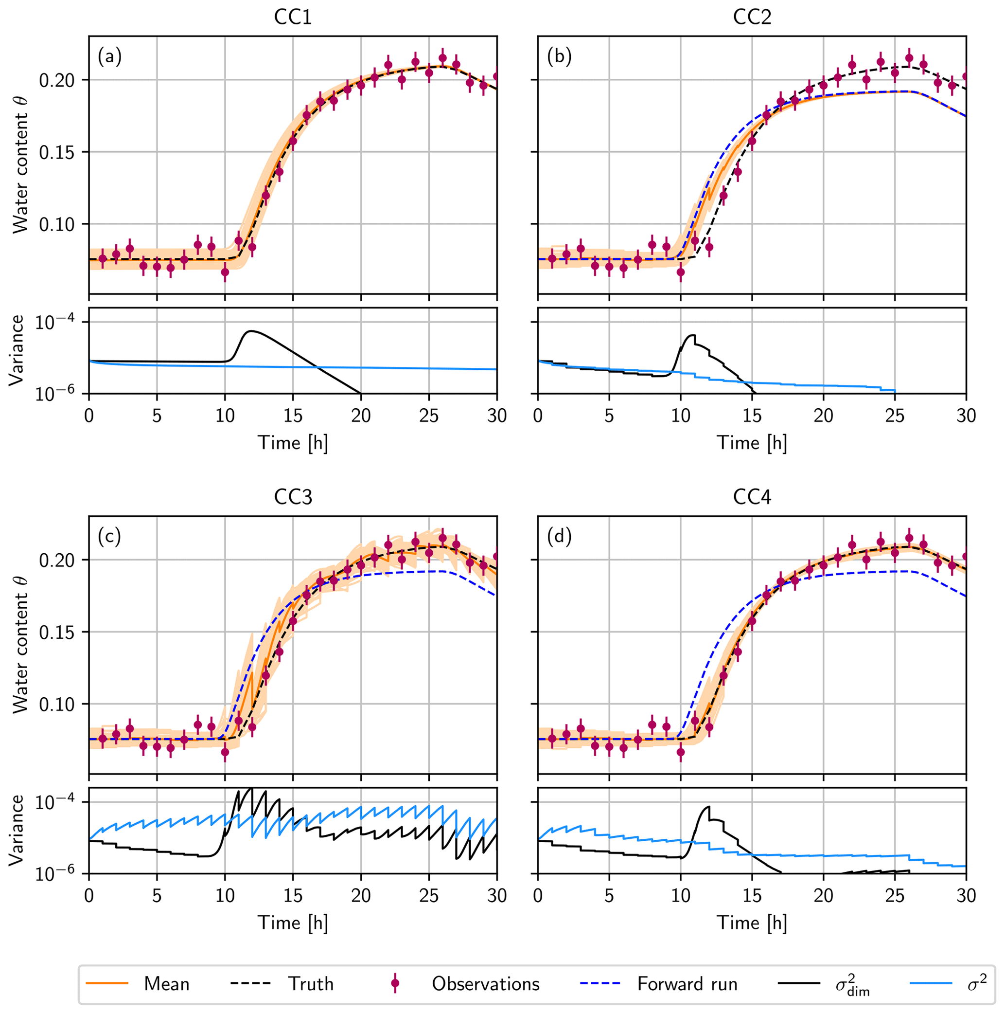
Figure 3 (a) Convergent case 1 (CC1) is the forward run without data assimilation, using an interpolated initial condition. In the other three cases, the truth is used to generate the initial ensemble. (b) Convergent case 2 (CC2), where the ensemble is propagated with n=2.68 instead of n_true=2.28, and the state is estimated. (c) Convergent case 3 (CC3), where the parameter error is represented by the ensemble, using 𝒩(2.68,0.4²), and the state is estimated. (d) Convergent case 4 (CC4) with the simultaneous state and parameter estimation. In the upper plots (a–d), the ensemble mean (orange) and the ensemble (light orange lines) during the forward run at the depth of the uppermost observation (20 cm). The truth, which is used to generate the observations (purple), is shown as a black dashed line. Panels (b–d) additionally show a single forward run (blue dashed line), using a wrong parameter n=2.68, starting from the true initial condition. In the lower plots (a–d), the mean variance σ² of the ensemble over all dimensions (light blue line) and variance ${\mathit{\sigma }}_{\dim }^{\mathrm{2}}$ at the depth of 20 cm (black line).

The ensemble variance at this depth ${\mathit{\sigma }}_{\dim }^{\mathrm{2}}$ increases when the infiltration front reaches 20 cm. Because of the nonlinear conductivity function (Eq. 9), the different initial water contents lead to a different arrival time of the infiltration front at the first observation position. This leads to an increase in the ensemble spread.

After the increase in the water content, the ensemble collapses fast since the hydraulic conductivity increases with the water content, which leads to a fast convergence of the different ensemble members to the truth due the convergent nature of the model. The variance over all dimensions σ² decreases slowly and approaches zero over time. If the system is started with a higher water content instead of equilibrium, this collapse will occur faster.

This case shows that a perfectly convergent system is predictable for all times. This is in contrast with divergent systems that only have a finite limit of predictability, even if the model, including boundary conditions, is perfectly known. After a transient phase, the states converge to the truth (Kalnay, 2003). A perfect model is not what we encounter in reality, however.

4.2.2 Convergent case 2 (CC2) – state estimation and wrong parameter

In this case, the state is estimated with the EnKF, but the ensemble is propagated with a wrong parameter. Instead of n_true=2.28, n=2.68 is chosen. The mean for the initial state is chosen as the true initial water content.

In Fig. 3b (upper plot) the temporal development of the water content at the depth of the uppermost observation (20 cm) is shown. A larger n results in an earlier arrival of the infiltration front at the depth of 20 cm for the ensemble than for the truth. The EnKF tries to correct the ensemble but fails because its variance is too small and cannot represent the truth. Due to the convergent system, σ² decreases constantly, while ${\mathit{\sigma }}_{\dim }^{\mathrm{2}}$ decreases fast to zero after the infiltration front reaches the depth of 20 cm (see Fig. 3b; lower plot). This convergence leads to a false trust in the model, and the filter degenerates. Compared to a forward run without data assimilation, the EnKF can only improve the state estimation for a short time when the water content rises due to the infiltration front. Soon after, the ensemble coincides with the free forward run, and the estimated state shows no advantage any more.

This case illustrates that a wrong parameter in a convergent system can lead to filter degeneration. This is in direct contrast to DC2 (Fig. 2b), where the filter is still able to estimate the state. The behavior also differs from DC3 (Fig. 2c), where the observation interval in the Lorenz 96 model is too short, meaning that it cannot develop its full divergent behavior. There the filter can also degenerate for a wrong parameter, but the data assimilation is still able to improve the estimation compared to a free forward run since the ensemble never collapses entirely.

4.2.3 Convergent case 3 (CC3) – state estimation and represented error

In this case, the parameter error is represented with the ensemble, but the parameter is not estimated. Each ensemble member has a different parameter n. The parameters are Gaussian distributed with 𝒩(2.68,0.4²) so that the truth lies within 1 standard deviation. Since the model error is known in this synthetic case, we can create an ensemble that represents the model error adequately. Note that this is more difficult, or even impossible, in a real-world system. The mean for the initial state is chosen as the true initial water content.

Figure 3c (upper plot) shows the temporal development of the water content at a depth of 20 cm. The infiltration front reaches this depth at different times due to the different parameter n for each ensemble member. This increases the variance in the ensemble, both at this depth and overall (see Fig. 3c; lower plot). The variance increases rapidly between the observations, similar to the divergent cases. In this way, the ensemble spread stays large enough so that the EnKF can correct the states. The ensemble can follow and represent the truth. This behavior can also be observed for the divergent case DC4 with a short observation interval (Fig. 2d).

Representing the model error adds a divergent component to the ensemble for a convergent model. This allows the EnKF to correct the state and follow the truth. However, the predictability of the system decreases since each ensemble member converges to a different fixed point apart from the truth. To increase the predictability, parameter estimation is necessary.

4.2.4 Convergent case 4 (CC4) – state and parameter estimation

In this case, the error in the parameter n is not only represented but also estimated using the state augmentation method. The initial parameter set is, as in CC3, Gaussian distributed with 𝒩(2.68,0.4²) so that the truth is located within 1 standard deviation. Again, the mean for the initial state is chosen as the true initial water content.

The estimation of n is shown in Fig. 4. The ensemble converges rapidly to the truth because only one parameter is estimated, so every deviation from the truth is mainly caused by this parameter.

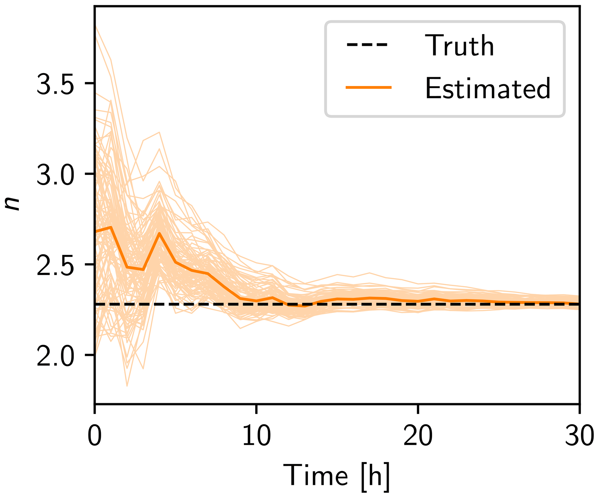
Figure 4 Estimation of parameter n in convergent case 4 (CC4). The ensemble mean is shown in orange and the ensemble in light orange. The truth is a black dashed line.

The mean variance σ² increases initially (Fig. 3d; lower plot) because, at the beginning, the parameter has not been sufficiently improved, and the ensemble members still have different n. This leads to a divergent ensemble in state space during the infiltration, which is similar to CC3. While the parameter is estimated, the variance of the ensemble decreases fast, and the convergent property of the system becomes dominant.

The temporal development of the water content at a depth of 20 cm is shown in Fig. 3d (upper plot). In contrast to CC3, the corrections of the EnKF to the state are much smaller. The mean of the parameter n comes close to the true value, and the uncertainty of n decreases. This causes the forward propagation to come close to the true model as well. The propagation with an almost correct model supports the state estimation due to the convergent nature of the system, which forces the state to the true value.

5 Discussion

For the divergent Lorenz 96 system, the EnKF is able to estimate the state for the true model as well as for the case with a wrong parameter. In a divergent system, the volume of the prior distribution in the state space increases during forward propagation (Evensen, 1994). For the EnKF, this is directly connected to the ensemble spread, which increases rapidly between the observations. This prevents a collapse of the ensemble even in the presence of an unrepresented parameter error. However, if the observation interval is too small relative to the characteristic time for divergence, the EnKF leads to a decrease in the ensemble spread such that the filter degenerates in the case of an unrepresented parameter error. Nevertheless, the divergent behavior of the model prevents a complete collapse of the ensemble so that the filter is still able to improve the state in a limited way.

In the convergent soil hydrological system, the volume of the prior distribution decreases during forward propagation such that the prior becomes more certain, even without an observation and data assimilation. For a perfect model, the predictability and state estimation in a convergent model are trivial. The initial ensemble will converge to the truth after some time, even with a rough initial approximation. In this case, data assimilation is not necessary.

In the case of model errors, in our study realized through a wrong parameter, the situation is different. The ensemble converges to a wrong state, the filter degenerates, and data assimilation fails. Increasing the ensemble size can only improve the performance marginally since all ensemble members converge to the same fixed point.

Representing the parameter error by assigning each ensemble member a different parameter increases the divergence of the system, and the filter is able to estimate the state again. Between the observations, the ensemble spread increases rapidly because the ensemble members diverge to different fixed points apart from the truth. This results in a finite predictability. By representing the parameter error, the Richards equation gains a divergent part similar to the Lorenz 96 model. In the case of a convergent system, it is necessary to represent the parameter error, otherwise the ensemble collapses.

To increase the predictability of the system again, it is necessary to not only represent but also to reduce the parameter uncertainty. In synthetic cases without model structural errors, the convergent property of the system supports the state estimation, and the predictability increases if the parameter estimation is successful. This shows the importance of parameter estimation for convergent systems. For divergent systems, parameter estimation also increases the predictability but only up to a point because predictability is limited by the system's dynamics.

For the application of data assimilation to real data, model errors typically cannot be attributed to unknown parameters or uncertainties in boundary conditions alone but also stem from model structural errors, like a simplified representation of sub-scale physics or unrepresented processes in the dynamics. Uncertainties in parameters and boundary conditions can be represented in an ensemble, but representing model structural errors is challenging or can be impossible. For example, in hydrology, the model errors are typically ill-known (Li and Ren, 2011) and can vary both in space and time, which then can lead to filter degeneracy and biased parameter estimation (Berg et al., 2019). While divergent models can alleviate the effect of an unrepresented error within certain bounds, in a convergent system it is necessary to represent all relevant model errors sufficiently to prevent filter degeneracy and enable an optimal state and parameter estimation. Since this is challenging or even impossible, heuristic ways to address filter degeneracy are necessary.

A practical alternative to increase the ensemble spread and avoid filter degeneracy is to use inflation methods. For example, keeping a constant ensemble spread for the parameters can provide a sufficient spread in state space (Zhang et al., 2017). The advantage is that this approach is a model-specific inflation and avoids the over-amplification of spurious correlations (Constantinescu et al., 2007). The disadvantage is that the EnKF is prevented from reducing the prediction uncertainty. This behavior is also shown in CC3. In this case, the ensemble spread in the parameter space adds a divergent component to the ensemble that results in an increased ensemble spread in state space and prevents filter degeneracy.

Multiplicative inflation increases the ensemble spread through an inflation factor (Anderson and Anderson, 1999). In a divergent system a small multiplicative inflation is sufficient to increase the existing ensemble spread. In a convergent system this requires a larger inflation and can lead to the over-inflation of spurious correlations (Constantinescu et al., 2007). To avoid this and to cope with spatial and temporal varying model errors, the use of more sophisticated adaptive inflation methods (e.g. Bauser et al., 2018; Gharamti, 2018) may be necessary in convergent systems.

Heuristic inflation methods cannot fully replace the representation of model errors and, hence, must be used judiciously. They can lead to the over-inflation of spurious correlations and can lead to biases in the estimation of parameters. If unrepresented model errors can be identified and are limited in space or time, these biases can be prevented by using a closed-eye period for the extent of the unrepresented model errors. In the closed-eye period, parameters are kept constant, and only the state is estimated, which can require inflation methods for a successful state estimation. This enables an improved parameter estimation without compensating for the unrepresented model dynamics though biased parameters outside of the closed-eye period, when and where uncertainties can be represented. The use of the closed-eye period in combination with the representation of relevant uncertainties has already been demonstrated in hydrology (Bauser et al., 2016).

6 Conclusions

We demonstrated the differences in and challenges of ensemble data assimilation for divergent and convergent systems on the example of the EnKF applied to the divergent Lorenz 96 model and a convergent soil water movement model based on the Richards equation.

Sequential ensemble data assimilation methods require a sufficient divergent part in the ensemble to maintain an adequate ensemble spread and prevent filter degeneration. In divergent systems, this is inherent to the system, provided that observation intervals and divergence times match. In convergent systems, relevant model errors must be represented to increase the ensemble spread and to, thereby, add a divergent part to the ensemble to avoid filter degeneracy. If errors stem from unknown parameters, estimating the parameters improves state estimation. However, this will reduce the ensemble spread again and require the remaining relevant model errors to be represented. Since this can be challenging, increasing the model errors artificially, by limiting the reduction of parameter uncertainty or through inflation methods, can be required in convergent systems.

This paper highlights the challenges when transferring sequential ensemble data assimilation methods from divergent systems to convergent systems, which must be considered when applying data assimilation.