Technical Note: Improved partial wavelet coherency for understanding scale-specific and localized bivariate relationships in geosciences

Bivariate wavelet coherency is a measure of correlation between two variables in the location–scale (spatial data) or time–frequency (time series) domain. It is particularly suited to geoscience, where relationships between multiple variables differ with locations (times) and/or scales (frequencies) because of the various processes involved. However, it is well-known that bivariate relationships can be misleading when both variables are dependent on other variables. Partial wavelet coherency (PWC) has been proposed to detect scale-specific and localized bivariate relationships by excluding the effects of other variables but is limited to one excluding variable and provides no phase information. We aim to develop a new PWC method that can deal with multiple excluding variables and provide phase information. Both stationary and non-stationary artificial datasets with the response variable being the sum of five cosine waves at 256 locations are used to test the method. The new method was also applied to a free water evaporation dataset. Our results verified the advantages of the new method in capturing phase information and dealing with multiple excluding variables. Where there is one excluding variable, the new PWC implementation produces higher and more accurate PWC values than the previously published PWC implementation that mistakenly considered bivariate real coherence rather than bivariate complex coherence. We suggest the PWC method is used to untangle scale-specific and localized bivariate relationships after removing the effects of other variables in geosciences. The PWC implementations were coded with Matlab and are freely accessible (https://figshare.com/s/bc97956f43fe5734c784, last access: 14 January 2021).

1 Introduction

Geoscience data, such as the spatial distribution of soil moisture in undulating terrains and time series of climatic variables, usually consist of a variety of transient processes with different scales or frequencies that may be localized in space or time (Torrence and Compo, 1998; Si, 2008; Graf et al., 2014). For example, time series of air temperature usually fluctuate periodically at different scales (e.g., daily and yearly), but abrupt changes in air temperature (e.g., extremely high or low) may occur at certain time points as a result of extreme weather and climate events (e.g., heat and rain). Wavelet methods are widely used to detect localized features of geoscience data.

Wavelet analyses are based on the wavelet transform using the mother wavelet function, which expands spatial data (or time series) into location–scale (or time–frequency) space for identification of localized intermittent scales (or frequencies). For convenience, we will mainly refer to location and scale irrespective of spatial or time series data unless otherwise mentioned. Bivariate wavelet coherency (BWC) is widely accepted as a tool for detecting scale-specific and localized bivariate relationships in a range of areas in geoscience (Lakshmi et al., 2004; Si and Zeleke, 2005; Das and Mohanty, 2008; Polansky et al., 2010; Biswas and Si, 2011). The BWC partitions correlation between two variables into different locations and scales, which are different from the overall relationships at the sampling scale as shown by the traditional correlation coefficient. For example, BWC analysis indicated that soil water content of a hummocky landscape in the Canadian Prairies was negatively correlated with soil organic carbon content at a slope scale (50 m), but they were positively correlated at a watershed scale (120 m) in summer because of the different processes involved at different scales (Hu et al., 2017b). Because the positive correlation may cancel out with the negative one at different scales and/or locations, the traditional correlation coefficient between soil water content and soil organic carbon content does not differ significantly from zero, which can be misleading.

Recently, Hu and Si (2016) extended BWC to multiple wavelet coherence (MWC) that can be used to untangle multivariate (≥3 variables) relationships in multiple location–scale domains. This method has been successfully used in hydrology (Hu et al., 2017b; Nalley et al., 2019; Su et al., 2019; Gu et al., 2020; Mares et al., 2020) and other areas such as soil science (Centeno et al., 2020), environmental science (Zhao et al., 2018), meteorology (Song et al., 2020), and economics (Sen and Choudhury, 2020). The MWC application has shown that an increased number of predictor variables does not necessarily explain more variations in the response variable, partly because predictor variables are usually cross-correlated (Hu and Si, 2016). For the same reason, bivariate relationships can be misleading if the predictor variable is correlated with other variables that control the response variable. Partial correlation analysis is one such method to avoid the misleading relationships resulting from the interdependence between predictor and other variables (Kenney and Keeping, 1939). For example, soil water content of the root zone was found to be positively related to grass yield throughout the year in a small watershed on the Chinese Loess Plateau (Hu et al., 2017a). This was because higher grass yield usually coincided with finer soils that usually have higher water-holding capacity. After removing the effects of other factors including sand content, partial correlation analysis indicated that soil water content was negatively affected by grass yield during growing seasons and not affected by grass yield during non-growing seasons as expected. The study of Hu et al. (2017a) clearly demonstrated that partial correlation analysis can be an effective method to avoid misleading relationships between response (e.g., soil water content) and predictor variables (e.g., grass yield) when the latter was interdependent with other variables (e.g., sand content). However, the extension of partial correlation to the multiple location–scale domain is limited. In order to better understand the bivariate relationships at various scales and locations, BWC needs to be extended to partial wavelet coherency (PWC) by eliminating the effects of other variables.

BWC was extended to PWC by Mihanoviæ et al. (2009). Their method has been widely used in the areas of marine science (Ng and Chan, 2012a, b), meteorology (Tan et al., 2016; Rathinasamy et al., 2017), and economics (Aloui et al., 2018; Altarturi et al., 2018; Wu et al., 2020), as well as in the study of greenhouse gas emissions (Jia et al., 2018; Li et al., 2018; Mutascu and Sokic, 2020), among others. For example, PWC analysis indicated that the Southern Oscillation Index and Pacific Decadal Oscillation did not affect precipitation across India, while this was misinterpreted by the BWC analysis because of their interdependence on Niño 3.4, which affects precipitation (Rathinasamy et al., 2017). Unfortunately, the PWC implementation in many previous studies (Ng and Chan, 2012b; Rathinasamy et al., 2017; Aloui et al., 2018; Altarturi et al., 2018; Jia et al., 2018; Li et al., 2018; Mutascu and Sokic, 2020; Wu et al., 2020) was based on an incorrect Matlab code developed by Ng and Chan (2012a), who might have misinterpreted the equation of Mihanoviæ et al. (2009) and mistakenly used bivariate real coherence rather than bivariate complex coherence for calculating PWC. Moreover, Mihanoviæ et al. (2009) considered only one excluding variable (i.e., the variable that influences the response variable is excluded) and did not include the phase angle difference between response and predictor variables. The PWC values between response and predictor variables can still be misleading if more than one variable is interdependent with the predictor variable. This is especially true if these variables are correlated with the predictor variable at different locations and/or scales. Without phase information, it is hard to tell whether the correlation at a location and scale is positive or negative.

As an extension of previous studies (Mihanoviæ et al., 2009; Hu and Si, 2016), this paper aims to develop a PWC method that considers more than one excluding variable and provides phase information. This new method reveals the magnitude and type of bivariate relationships after removing the effects from all potentially interdependent variables. We expect that the new method will produce more accurate PWC values than the implementation of Ng and Chan (2012a), where there is one excluding variable. The new method is an extension of the multivariate partial coherency in the frequency (scale) domain (Koopmans, 1974). The proposed method is first tested with artificial datasets following Yan and Gao (2007) and Hu and Si (2016) to demonstrate its capability of capturing the known relationships of the artificial data. Then it is applied to a real dataset, i.e., time series of free water evaporation at the Changwu site in China (Hu and Si, 2016). Finally, the advantages and weaknesses of the new method are discussed by comparing it with the previous PWC method (Mihanoviæ et al., 2009) and implementation (Ng and Chan, 2012a).

2 Theory

Wavelet analysis is based on the wavelet transform, which includes continuous wavelet transform and discrete wavelet transform. While the discrete wavelet transform is mainly used for data compression and noise reduction, the continuous wavelet transform is widely used for extracting scale-specific and localized features, as in the case of this study (Grinsted et al., 2004). The wavelet transform decomposes the spatial data (or time series) into a set of location- and scale-specific wavelet coefficients, which are scaled (contracted or expanded) and shifted versions of mother wavelets. Different mother wavelets are available for wavelet transform, among which the Morlet wavelet, composed of a complex exponential multiplied by a Gaussian window, provides a good balance between location and scale localization. Therefore, continuous wavelet transform with the Morlet wavelet is suitable for transforming spatial data (or time series) into a location–scale (or time–frequency) domain, which allows us to identify both location-specific amplitude and phase information of wavelet coefficients at different scales (Torrence and Compo, 1998). Wavelet coefficients and their complex conjugates are used to calculate auto-wavelet power spectra and cross-wavelet power spectra. BWC is calculated as the ratio of smoothed cross-wavelet power spectra of two variables to the product of their auto-wavelet power spectra (Grinsted et al., 2004). Hu and Si (2016) extended wavelet coherence from two to multiple (≥3) variables and developed MWC. Detailed information on the calculations of wavelet coefficients, auto- and cross-wavelet power spectra, BWC, and MWC based on the continuous wavelet transform can be found in previous studies (e.g., Torrence and Compo, 1998; Grinsted et al., 2004; Si and Farrell, 2004; Si, 2008; Hu and Si, 2016; Hu et al., 2017b). Here, we will only introduce the theory and calculation that are most relevant to PWC.

Similarly to BWC and MWC, PWC is calculated from auto- and cross-wavelet power spectra, for the response variable y, predictor variable x, and excluding variables Z ($Z=\left\{Z_{\mathrm{1}},Z_{\mathrm{2}},\mathrm{\dots },Z_q\right\})$. Koopmans (1974) developed the multivariate complex PWC in the frequency (scale) domain. Here, we extend the Koopmans (1974) method from the frequency (scale) domain to the time–frequency (location–scale) domain. Therefore, the complex PWC between y and x after excluding variables Z at scale s and location τ, ${\mathit{\gamma }}_{y,x\cdot Z}(s,\mathit{\tau })$, can be written as

$$\begin{array}{}\text{(1)}& {\mathit{\gamma }}_{y,x\cdot Z}(s,\mathit{\tau })={\displaystyle \frac{\left(\mathrm{1}-R_{y,x,Z}^{\mathrm{2}}(s,\mathit{\tau })\right){\mathit{\gamma }}_{y,x}(s,\mathit{\tau })}{\sqrt{\left(\mathrm{1}-R_{y,Z}^{\mathrm{2}}(s,\mathit{\tau })\right)\left(\mathrm{1}-R_{x,Z}^{\mathrm{2}}(s,\mathit{\tau })\right)}}},\end{array}$$

where symbol ⋅ is the notation for excluding variables; $R_{y,x,Z}^{\mathrm{2}}(s,\mathit{\tau })$, $R_{y,Z}^{\mathrm{2}}(s,\mathit{\tau })$, and $R_{x,Z}^{\mathrm{2}}(s,\mathit{\tau })$ can be calculated by following Hu and Si (2016) as

$$\begin{array}{}\text{(2)}& {\displaystyle }{R}_{y,x,Z}^{\mathrm{2}}(s,\mathit{\tau })={\displaystyle \frac{{\overleftrightarrow{w}}^{y,Z}(s,\mathit{\tau }){\overleftrightarrow{w}}^{Z,Z}(s,\mathit{\tau }{)}^{-\mathrm{1}}\stackrel{\mathrm{‾}}{{\overleftrightarrow{w}}^{x,Z}(s,\mathit{\tau })}}{{\overleftrightarrow{w}}^{y,x}(s,\mathit{\tau })}},\text{(3)}& {\displaystyle }{R}_{y,Z}^{\mathrm{2}}(s,\mathit{\tau })={\displaystyle \frac{{\overleftrightarrow{w}}^{y,Z}(s,\mathit{\tau }){\overleftrightarrow{w}}^{Z,Z}(s,\mathit{\tau }{)}^{-\mathrm{1}}\stackrel{\mathrm{‾}}{{\overleftrightarrow{w}}^{y,Z}(s,\mathit{\tau })}}{{\overleftrightarrow{w}}^{y,y}(s,\mathit{\tau })}},\text{(4)}& {\displaystyle }{R}_{x,Z}^{\mathrm{2}}(s,\mathit{\tau })={\displaystyle \frac{{\overleftrightarrow{w}}^{x,Z}(s,\mathit{\tau }){\overleftrightarrow{w}}^{Z,Z}(s,\mathit{\tau }{)}^{-\mathrm{1}}\stackrel{\mathrm{‾}}{{\overleftrightarrow{w}}^{x,Z}(s,\mathit{\tau })}}{{\overleftrightarrow{w}}^{x,x}(s,\mathit{\tau })}}.\end{array}$$

Equation (1) can also be derived analogously from the complex partial spectrum for the frequency domain according to the definition of complex coherence between two variables in the time–frequency domain (see Sect. S1 in the Supplement for the derivation process). Note that $R_{y,x,Z}^{\mathrm{2}}(s,\mathit{\tau })$ is a matrix with complex values, while $R_{y,Z}^{\mathrm{2}}(s,\mathit{\tau })$ and $R_{x,Z}^{\mathrm{2}}(s,\mathit{\tau })$ are matrices with real numbers. ${\mathit{\gamma }}_{y,x}(s,\mathit{\tau })$ is the complex wavelet coherence between y and x, which can be written as

$$\begin{array}{}\text{(5)}& {\mathit{\gamma }}_{y,x}(s,\mathit{\tau })={\displaystyle \frac{{\overleftrightarrow{w}}^{y,x}(s,\mathit{\tau })}{\sqrt{\left({\overleftrightarrow{w}}^{y,y}(s,\mathit{\tau }){\overleftrightarrow{w}}^{x,x}(s,\mathit{\tau })\right)}}},\end{array}$$

where $\overleftrightarrow{\left(\right)}$ is the smoothing operator, $\stackrel{\mathrm{‾}}{\left(\right)}$ is the complex conjugate operator, ( )⁻¹ indicates the inverse of the matrix, and

$$\begin{array}{}\text{(6)}& {\displaystyle }{\overleftrightarrow{w}}^{y,Z}(s,\mathit{\tau })& {\displaystyle }=\left[{\overleftrightarrow{w}}^{y,Z_{\mathrm{1}}}(s,\mathit{\tau }){\overleftrightarrow{w}}^{y,Z_{\mathrm{2}}}(s,\mathit{\tau })\mathrm{\dots }{\overleftrightarrow{w}}^{y,Z_q}(s,\mathit{\tau })\right],\text{(7)}& {\displaystyle }{\overleftrightarrow{w}}^{x,Z}(s,\mathit{\tau })& {\displaystyle }=\left[{\overleftrightarrow{w}}^{x,Z_{\mathrm{1}}}(s,\mathit{\tau }){\overleftrightarrow{w}}^{x,Z_{\mathrm{2}}}(s,\mathit{\tau })\mathrm{\dots }{\overleftrightarrow{w}}^{x,Z_q}(s,\mathit{\tau })\right],\text{(8)}& {\displaystyle }{\overleftrightarrow{w}}^{Z,Z}(s,\mathit{\tau })& {\displaystyle }=\left[\begin{array}{ccc}{\overleftrightarrow{w}}^{Z_{\mathrm{1}},Z_{\mathrm{1}}}(s,\mathit{\tau })& \mathrm{\cdots }& {\overleftrightarrow{w}}^{Z_{\mathrm{1}},Z_q}(s,\mathit{\tau })\\ \mathrm{⋮}& \mathrm{\ddots }& \mathrm{⋮}\\ {\overleftrightarrow{w}}^{Z_q,Z_{\mathrm{1}}}(s,\mathit{\tau })& \mathrm{\cdots }& {\overleftrightarrow{w}}^{Z_q,Z_q}(s,\mathit{\tau })\end{array}\right],\end{array}$$

where ${\overleftrightarrow{w}}^{A,B}(s,\mathit{\tau })$ is the smoothed auto-wavelet power spectra (when A=B) or cross-wavelet power spectra (when A≠B) at scale s and location τ, respectively.

The squared PWC (hereinafter referred to as PWC) at scale s and location τ, ${\mathit{\rho }}_{y,x\cdot Z}^{\mathrm{2}}$, can be written as

$$\begin{array}{}\text{(9)}& {\mathit{\rho }}_{y,x\cdot Z}^{\mathrm{2}}={\displaystyle \frac{{\left|\mathrm{1}-R_{y,x,Z}^{\mathrm{2}}(s,\mathit{\tau })\right|}^{\mathrm{2}}{R}_{y,x}^{\mathrm{2}}(s,\mathit{\tau })}{\left(\mathrm{1}-R_{y,Z}^{\mathrm{2}}(s,\mathit{\tau })\right)\left(\mathrm{1}-R_{x,Z}^{\mathrm{2}}(s,\mathit{\tau })\right)}},\end{array}$$

where $R_{y,x}^{\mathrm{2}}(s,\mathit{\tau })$ is squared BWC between y and x, which can be expressed as

$$\begin{array}{}\text{(10)}& R_{y,x}^{\mathrm{2}}(s,\mathit{\tau })={\displaystyle \frac{{\overleftrightarrow{w}}^{y,x}(s,\mathit{\tau })\stackrel{\mathrm{‾}}{{\overleftrightarrow{w}}^{y,x}(s,\mathit{\tau })}}{{\overleftrightarrow{w}}^{y,y}(s,\mathit{\tau }){\overleftrightarrow{w}}^{x,x}(s,\mathit{\tau })}}.\end{array}$$

The phase angle (i.e., angle between two complex numbers) between y and x after the excluding effect of Z is

$$\begin{array}{}\text{(11)}& {\mathit{\vartheta }}_{y,x\cdot Z}(s,\mathit{\tau })={\mathit{\phi }}_{y,x\cdot Z}(s,\mathit{\tau })+{\mathit{\vartheta }}_{y,x}(s,\mathit{\tau }),\end{array}$$

where

$$\begin{array}{}\text{(12)}& {\mathit{\phi }}_{y,x\cdot Z}(s,\mathit{\tau })=\text{arg}\left(\mathrm{1}-R_{y,x,Z}^{\mathrm{2}}(s,\mathit{\tau })\right),\end{array}$$

and ${\mathit{\vartheta }}_{y,x}(s,\mathit{\tau })$ is the wavelet phase between y and x, which can be expressed as

$$\begin{array}{}\text{(13)}& {\mathit{\vartheta }}_{y,x}(s,\mathit{\tau })={\tan }^{-\mathrm{1}}\left(\text{Im}\left(W^{y,x}(s,\mathit{\tau })\right)/\text{Re}\left(W^{y,x}(s,\mathit{\tau })\right)\right),\end{array}$$

where arg denotes the argument of the complex number and $W^{y,x}(s,\mathit{\tau })$ is the cross-wavelet power spectrum between y and x at scale s and location τ; Im and Re denote the imaginary and real parts of $W^{y,x}(s,\mathit{\tau })$, respectively.

When only one variable (e.g., Z₁) is excluded, Eq. (9) can be written as (see Sect. S2 in the Supplement for the derivation process)

$$\begin{array}{}\text{(14)}& {\mathit{\rho }}_{y,x\cdot Z_{\mathrm{1}}}^{\mathrm{2}}={\displaystyle \frac{{\left|{\mathit{\gamma }}_{y,x}(s,\mathit{\tau })-{\mathit{\gamma }}_{y,Z_{\mathrm{1}}}(s,\mathit{\tau })\stackrel{\mathrm{‾}}{{\mathit{\gamma }}_{x,Z_{\mathrm{1}}}(s,\mathit{\tau })}\right|}^{\mathrm{2}}}{\left(\mathrm{1}-R_{y,Z_{\mathrm{1}}}^{\mathrm{2}}(s,\mathit{\tau })\right)\left(\mathrm{1}-R_{x,Z_{\mathrm{1}}}^{\mathrm{2}}(s,\mathit{\tau })\right)}}.\end{array}$$

The widely used Monte Carlo method (Torrence and Compo, 1998; Grinsted et al., 2004; Si and Farrell, 2004) is used to calculate PWC at the 95 % confidence level. In brief, the PWC calculation is repeated for a sufficient number (i.e., minimum number required) of times using data generated by Monte Carlo simulations based on the first-order autocorrelation coefficient (r1). The first-order autoregressive model (AR(1)) is chosen because most geoscience data can be effectively simulated by it (Wendroth et al., 1992; Grinsted et al., 2004; Si and Farrell, 2004), although we recognize that a time series with long-range dependence is also common in many areas such as hydrology (Szolgayová et al., 2014). Different combinations of r1 values (i.e., 0.0, 0.5, and 0.9) were used to generate 10 to 10 000 AR(1) series with three, four, and five variables. Our results indicate that the noise combination has little impact on the PWC values at the 95 % confidence level as also found by Grinsted et al. (2004) for the BWC case (data not shown). The relative difference of PWC at the 95 % confidence level compared with that calculated from the 10 000 AR(1) series decreases with the increase in number of AR(1) series (Fig. S1 of Sect. S3 in the Supplement). When the number of AR(1) is above 300, a very low maximum relative difference (e.g., <2 %) is observed. Therefore, a repeating number of 300 seems to be sufficient for a significance test. However, if calculation time is not a barrier, a higher repeating number, such as ≥1000, is recommended. The 95th percentile of PWCs of all simulations at each scale represents PWC at the 95 % confidence level. The average PWC, percent area of significant coherence (PASC) relative to the whole wavelet location–scale domain (Hu and Si, 2016), and average value of significant PWC (PWC_sig) are also calculated for different location–scale domains.

In the case of one excluding variable (Z={Z₁}), Mihanoviæ et al. (2009) suggested that PWC can be calculated by an equation analogous to the traditional partial correlation squared (Kenney and Keeping, 1939) without giving a detailed derivation process. Their equation is the same as Eq. (14). Unfortunately, Ng and Chan (2012a) might have misinterpreted the equation of Mihanoviæ et al. (2009) and developed Matlab code for calculating PWC using the equation expressed as

$$\begin{array}{}\text{(15)}& {\mathit{\rho }}_{y,x\cdot Z_{\mathrm{1}}}^{\mathrm{2}}={\displaystyle \frac{{\left|R_{y,x}(s,\mathit{\tau })-R_{y,Z_{\mathrm{1}}}(s,\mathit{\tau })R_{x,Z_{\mathrm{1}}}(s,\mathit{\tau })\right|}^{\mathrm{2}}}{\left(\mathrm{1}-R_{y,Z_{\mathrm{1}}}^{\mathrm{2}}(s,\mathit{\tau })\right)\left(\mathrm{1}-R_{x,Z_{\mathrm{1}}}^{\mathrm{2}}(s,\mathit{\tau })\right)}},\end{array}$$

where $R_{y,x}(s,\mathit{\tau })$, $R_{y,Z_{\mathrm{1}}}(s,\mathit{\tau })$, and $R_{x,Z_{\mathrm{1}}}(s,\mathit{\tau })$ are the square roots of $R_{y,x}^{\mathrm{2}}(s,\mathit{\tau })$, $R_{y,Z_{\mathrm{1}}}^{\mathrm{2}}(s,\mathit{\tau })$, and $R_{x,Z_{\mathrm{1}}}^{\mathrm{2}}(s,\mathit{\tau })$, respectively. $R_{y,Z_{\mathrm{1}}}^{\mathrm{2}}(s,\mathit{\tau })$ and $R_{x,Z_{\mathrm{1}}}^{\mathrm{2}}(s,\mathit{\tau })$ can be calculated from Eq. (10) by replacing y and x with their corresponding variables. Equation (15) has been widely used to calculate PWC in the case of one excluding variable (Ng and Chan, 2012b; Rathinasamy et al., 2017; Aloui et al., 2018; Altarturi et al., 2018; Jia et al., 2018; Li et al., 2018; Mutascu and Sokic, 2020; Wu et al., 2020). Note that complex coherence and real coherence are involved in the numerators of Eqs. (14) and (15), respectively, while the denominators are exactly the same. Further comparison indicates that Eq. (15) underestimates PWC value relative to Eq. (14) unless ${\mathit{\gamma }}_{y,x}(s,\mathit{\tau })$ and ${\mathit{\gamma }}_{y,Z_{\mathrm{1}}}(s,\mathit{\tau })\stackrel{\mathrm{‾}}{{\mathit{\gamma }}_{x,Z_{\mathrm{1}}}(s,\mathit{\tau })}$ in Eq. (14) are collinear (i.e., their arguments are identical) under which the two equations produce the same PWC values. Differences between Eqs. (14) and (15) will be discussed further using both artificial data and a real dataset. For comparison purposes, we refer to Eqs. (14) and (15) as the new implementation and the classical implementation, respectively.

3 Method test using artificial data

3.1 Artificial data and analysis

PWC is first tested using the cosine-like artificial dataset produced following Yan and Gao (2007). The cosine-like artificial datasets are suitable for testing the new method because they mimic many spatial or time series data in geoscience such as climatic variables, hydrologic fluxes, seismic signals, El Niño–Southern Oscillation, land surface topography, ocean waves, and soil moisture. The procedures to test PWC are largely based on Hu and Si (2016), where the same dataset has been used to test the MWC method (refer to Hu and Si, 2016, for a detailed description of the artificial dataset). The response variable (y and z for the stationary and non-stationary cases, respectively) is the sum of five cosine waves (y₁ to y₅ and z₁ to z₅ for the stationary and non-stationary cases, respectively) at 256 locations (Hu and Si, 2016). For y₁ to y₅, they have consistent dimensionless scales of 4, 8, 16, 32, and 64, respectively, across the series. From z₁ to z₅, the dimensionless scales gradually change with location, with the maximum dimensionless scales of 4, 8, 16, 32, and 64, respectively. The variance of the response variables y and z is 2.5. All other variables are orthogonal to each other with equal variance of 0.5. The predictor and excluding variables (Fig. S2 of Sect. S3 in the Supplement) are selected from two of the five cosine waves (i.e., y₂ and y₄ or z₂ and z₄) and/or their derivatives. The exact variables and procedures to test the new PWC method are explained below.

First, PWC between response variable y (or z) and predictor variable, i.e., y₂ (or z₂), is calculated after excluding the effect of one variable. Four types of excluding variable are involved (Fig. S2 of Sect. S3 in the Supplement): (a) original series of y₄ (or z₄); (b) second halves of the original series of y₂ (or z₂) are replaced by 0 to simulate abrupt changes (i.e., transient and localized feature) in the spatial data. They are referred to as y_2,h0 (or z_2,h0); (c) white noises with zero-mean and standard deviations of 0.3 (weak noise), 1 (moderate noise), and 4 (high noise) are added to y₂ (or z₂) as suggested by Hu and Si (2016) to simulate non-perfect cyclic patterns of the excluding variables. They are referred to as y_2,w (or z_2,w), y_2,m (or z_2,m), and y_2,s (or z_2,s), respectively; and (d) a combination of type b and type c. They are referred to as $y_{\mathrm{2},\mathrm{w},\mathrm{h}\mathrm{0}}$ (or $z_{\mathrm{2},\mathrm{w},\mathrm{h}\mathrm{0}})$, $y_{\mathrm{2},\mathrm{m},\mathrm{h}\mathrm{0}}$ (or $z_{\mathrm{2},\mathrm{m},\mathrm{h}\mathrm{0}}$), and $y_{\mathrm{2},\mathrm{s},\mathrm{h}\mathrm{0}}$ (or $z_{\mathrm{2},\mathrm{s},\mathrm{h}\mathrm{0}}$), respectively.

Second, PWC between response variable y (or z) and predictor variable, i.e., y₂₄ (sum of y₂ and y₄) for the stationary case or z₂₄ (sum of z₂ and z₄) for the non-stationary case, is calculated with two excluding variables, which is a combination of y₄ (or z₄) and y₂ (or z₂) or its noised series (y_2,w or z_2,w, y_2,m or z_2,m, and y_2,s or z_2,s).

The merit of the artificial data is that we know the exact scale-specific and localized bivariate relationships after the effect of excluding variables is removed. Theoretically, we expect that (a) PWC is 1 at scales corresponding to the relative complement of excluding variable scales in predictor variable scales and 0 at other scales. For example, PWC between y and y₂₄ after excluding the effect of y₄ is expected to be 1 at the scale of 8, which is the relative complement of scale of excluding variable y₄ (32) in scales of predictor variable y₂₄ (8 and 32), and 0 at other scales; (b) PWC remains 1 in the second half of series, where spatial series is replaced by 0, and is 0 at the first half of the original series. For example, PWC between y and y₂ after excluding the effect of y_2,h0 is expected to be 0 and 1 in the first and second halves of series, respectively, at the scale of 8; and (c) PWC increases as more noises are included in the excluding variables. For example, PWC between y and y₂ after excluding the effect of noised series of y₂ is expected to increase with increasing noises in an order of $y_{\mathrm{2},\mathrm{w}}<y_{\mathrm{2},\mathrm{m}}<y_{\mathrm{2},\mathrm{s}}$ at the scale of 8.

3.2 PWC with artificial data

3.2.1 PWC with one excluding variable using the new method

Figure 1 shows PWC between response variable y (or z) and predictor variable y₂ (or z₂) by excluding one variable. For the stationary case, there is one horizontal band (red color) representing an in-phase high PWC value at scales around 8 for all locations after eliminating the effect of y₄ (Fig. 1a). Note that the PWC values between y and y₂ after excluding the effect of y₄ are not exactly 1 as would be expected at all location–scale domains, because of the effect of smoothing along locations and scales. However, the PWC values at the center of the significance band, which corresponds to the predictor variable y₂ at exactly the scale of 8, are very close to 1 (0.996), and the mean PWC_sig values are very high (i.e., 0.96). The result is similar to the BWC between y and y₂ (data not shown). This is understandable because y₄ is orthogonal to y₂, and excluding the effect of y₄ does not affect the relationship between y and y₂ at all.

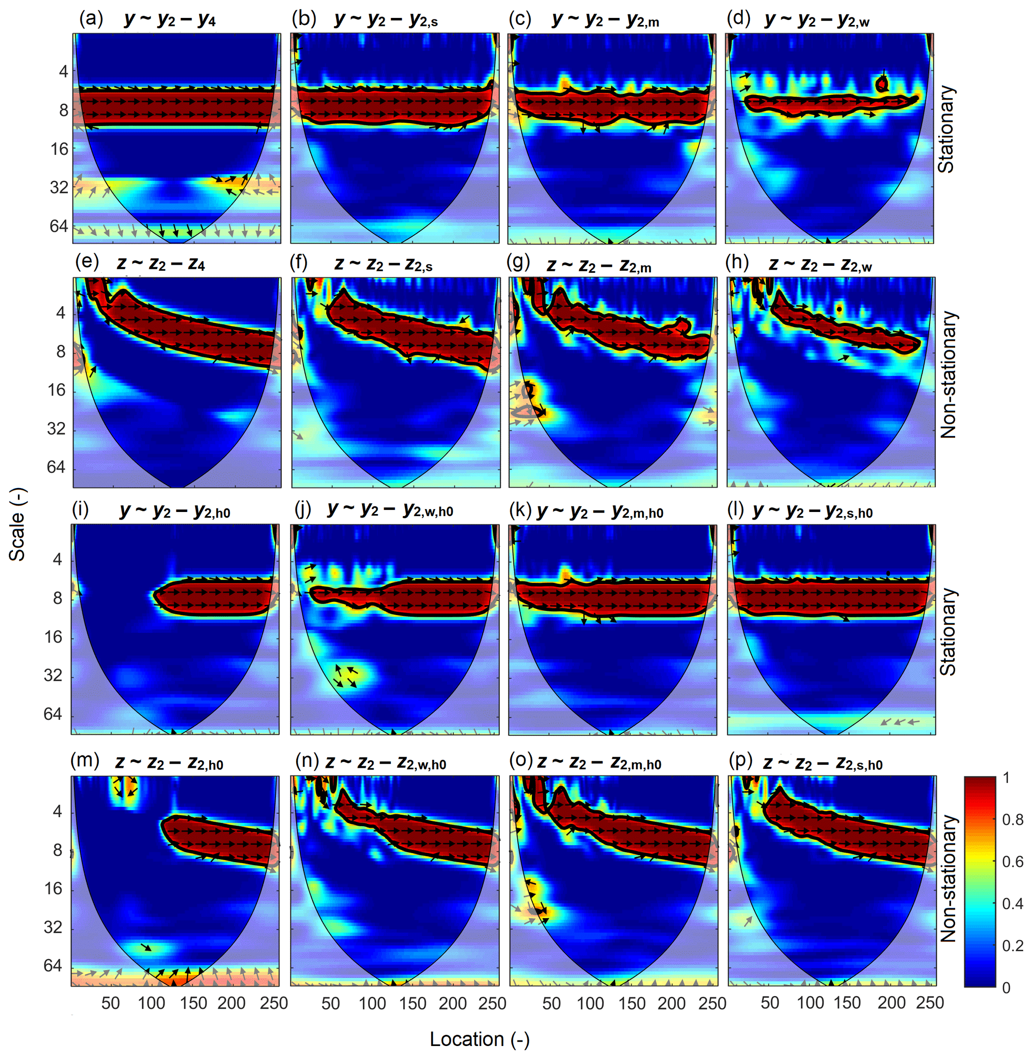
Figure 1 Partial wavelet coherency (PWC) between response variable y (or z) and predictor variable y₂ (or z₂) after excluding the effect of variables y₄ (or z₄), y_2,s (or z_2,s), y_2,m (or z_2,m), y_2,w (or z_2,w), y_2,h0 (or z_2,h0), $y_{\mathrm{2},\mathrm{w},\mathrm{h}\mathrm{0}}$ (or $z_{\mathrm{2},\mathrm{w},\mathrm{h}\mathrm{0}}$), $y_{\mathrm{2},\mathrm{m},\mathrm{h}\mathrm{0}}$ (or $z_{\mathrm{2},\mathrm{m},\mathrm{h}\mathrm{0}}$), and $y_{\mathrm{2},\mathrm{s},\mathrm{h}\mathrm{0}}$ (or $z_{\mathrm{2},\mathrm{s},\mathrm{h}\mathrm{0}}$) for the stationary (or non-stationary) case using the new method. Arrows represent the phase angles of the cross-wavelet power spectra between two variables after eliminating the effect of excluding variables. Arrows pointing to the right (left) indicate positive (negative) correlations. Thin and thick solid lines show the cones of influence and the 95 % confidence levels, respectively. All variables were generated by following Yan and Gao (2007) and Hu and Si (2016) and are explained in Sect 3.1 and shown in Fig. S2 of Sect. S3 in the Supplement.

Compared with the case of the excluding variable of y₄ (Fig. 1a), excluding the effect of y_2,s (Fig. 1b) results in a slightly narrower band of significant PWC and slightly reduced mean PWC_sig (0.94 versus 0.96). When less noise is included in the excluding variables (i.e., y_2,m and y_2,w) (Fig. 1c and d), the significant PWC band becomes narrower. The PASC values are 86 %, 77 %, and 32 % for excluding y_2,s, y_2,m, and y_2,w, respectively, at scales of 6–10. Moreover, the mean PWC_sig decreases from 0.94 (y_2,s) to 0.93 (y_2,m) and 0.89 (y_2,w) when progressively less noise is added (Fig. 1b–d). For the non-stationary case, similar results are obtained (Fig. 1e–h). The only difference is that the scales with significant PWC values change with location, as is found for MWC (Hu and Si, 2016).

When the second half of the excluding variable series is replaced by 0, the PWC values in that half are close to 1, while those in the first half of the data series are 0 at scales corresponding to the predictor variable (Fig. 1i and m). For the stationary case, after excluding the effect of y_2,h0, the PWC values are close to 1 (0.98) and 0 in the second and first halves of the data series, respectively, at the dimensionless scale of 8 (Fig. 1i). Similar results are observed for the non-stationary case (Fig. 1m). This is anticipated because the series of 0s is independent of the predictor variable and hence has no effect on the correlations between response and predictor variables at these locations. If different magnitudes of noises are added to the first half of the excluding variables (y₂ or z₂), the significant PWC band in the first half becomes wider as the magnitude of noises increases, while the significant PWC band in the second half remains almost unchanged (Fig. 1j–l and n–p). In the stationary case, for example, the PASC values at scales of 6–10 are 40 % ($y_{\mathrm{2},\mathrm{w},\mathrm{h}\mathrm{0}}$), 74 % ($y_{\mathrm{2},\mathrm{m},\mathrm{h}\mathrm{0}}$), and 86 % ($y_{\mathrm{2},\mathrm{s},\mathrm{h}\mathrm{0}}$) in the first half, while those values vary from 86 % to 90 % in the second half (Fig. 1j–l). Meanwhile, the mean PWC_sig in the first half at scales of 6–10 increases from 0.91 to 0.94 in both the stationary (Fig. 1j–l) and non-stationary (Fig. 1n–p) cases as more noises are added to the excluding variables y₂ or z₂. This indicates that the new PWC method can also capture the abrupt changes (Fig. 1i and m) in the data series and has the ability to deal with localized relationships.

3.2.2 PWC with two excluding variables using the new method

When both y₂ and y₄ (or z₂ and z₄) are considered in the predictor variables, there are two bands of wavelet coherence of 1 between y (or z) and y₂₄ (or z₂₄) (Hu and Si, 2016), which correspond to the scales of two predictor variables. However, after the effect of y₄ (or z₄) is removed, only one band with PWC of around 1 occurs at the scale of the predictor variable y₂ (or z₂) (Fig. 2a and f). After both predictor variables y₂ and y₄ (or z₂ and z₄) are excluded (Fig. 2b and g), PWC between y (or z) and y₂₄ (or z₂₄) is 0 at all location–scale domains as expected. When one of the excluding variables y₂ (or z₂) is added with noises, the relationship between response variable y (or z) and predictor variable y₂₄ (or z₂₄) becomes significant at scales of the excluding variable y₂ (or z₂) (Fig. 2c and h). Similar to the case of one excluding variable (Fig. 1), less noise in the excluding variable of y₂ (or z₂) results in a narrower significant PWC band and reduced mean PWC_sig values, e.g., from 0.96 (y_2,s) to 0.90 (y_2,w) in the stationary case (Fig. 2c–e) and from 0.95 (z_2,s) to 0.92 (z_2,w) in the non-stationary case (Fig. 2h–j).

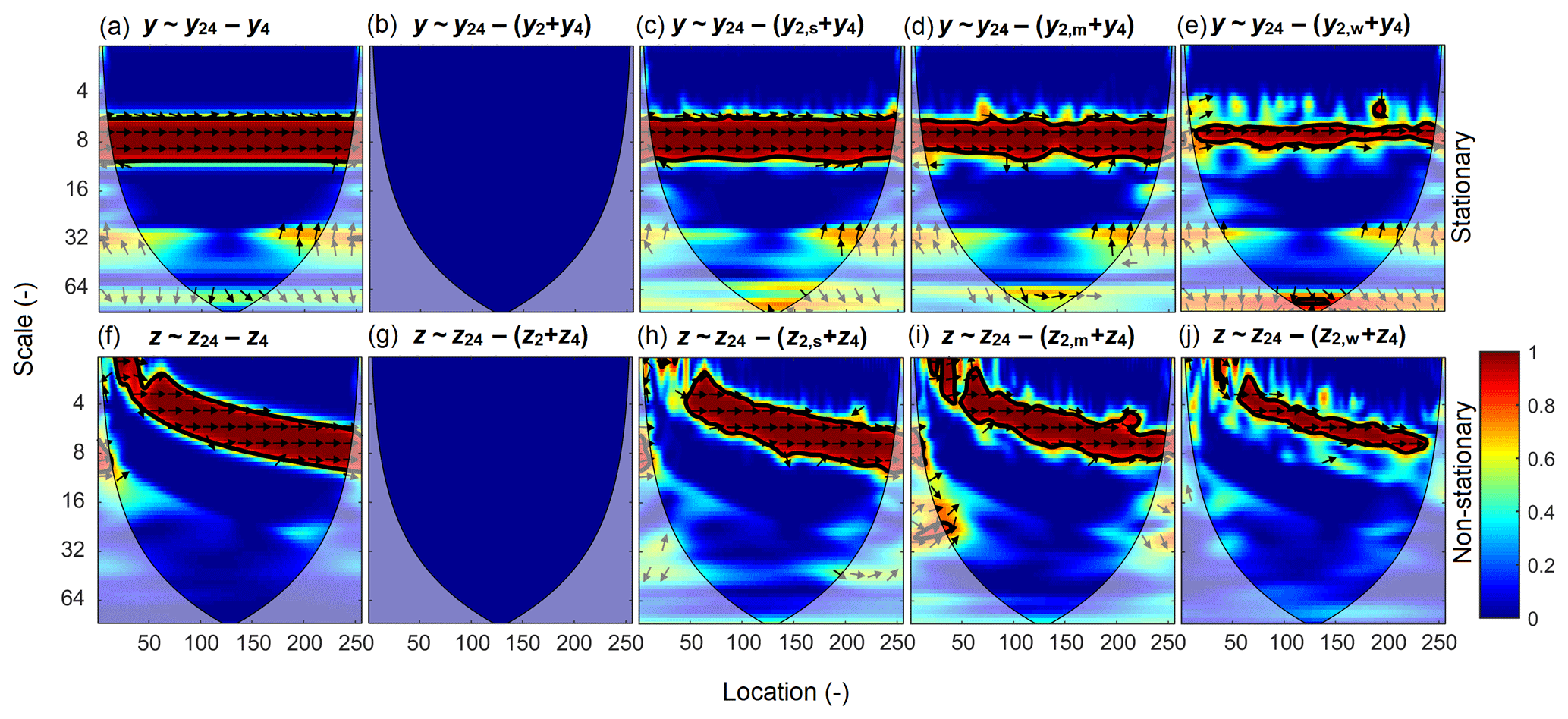
Figure 2 PWC between response variable y (or z) and predictor variable y₂₄ (or z₂₄) after excluding the effect of variables y₄ (or z₄), y₂+y₄ (or z₂+z₄), $y_{\mathrm{2},\mathrm{s}}+y_{\mathrm{4}}$ (or $z_{\mathrm{2},\mathrm{s}}+z_{\mathrm{4}}$), $y_{\mathrm{2},\mathrm{m}}+y_{\mathrm{4}}$ (or $z_{\mathrm{2},\mathrm{m}}+z_{\mathrm{4}}$), and $y_{\mathrm{2},\mathrm{w}}+y_{\mathrm{4}}$ (or $z_{\mathrm{2},\mathrm{w}}+z_{\mathrm{4}}$) for the stationary (or non-stationary) case using the new method. All variables were generated by following Yan and Gao (2007) and Hu and Si (2016) and are explained in Sect. 3.1 and shown in Fig. S2 of Sect. S3.

4 Method application with the real dataset

4.1 Description of the free water evaporation dataset

The free water evaporation dataset was used to test MWC (Hu and Si, 2016). In brief, this dataset includes monthly free water evaporation (E), mean temperature (T), relative humidity (RH), sun hours (SH), and wind speed (WS) between January 1979 and December 2013 at the Changwu site in Shaanxi province provided by the China Meteorological Administration. During this period, the average daily temperature was 9.4 ^∘C, the average annual rainfall was 571 mm, and annual potential evapotranspiration was 883 mm. Because of its location between semi-arid and subhumid climates, agricultural production at the Changwu site is constrained by water availability. Results of the wavelet power spectrum of E and BWC between every two variables are shown in Figs. S3 and S4 (Sect. S3 in the Supplement), respectively.

4.2 PWC with the free water evaporation dataset

The PWC analysis indicates that the correlations between E and T after excluding the effect of each of the other three variables (RH, SH, and WS) were almost the same as those indicated by BWC (Figs. 3a–c and S4 of Sect. S3 in the Supplement). For example, E and T, after excluding the effect of RH, were positively correlated at the medium scales (8–32 months). The PASC was 61 % and the mean PWC_sig value was 0.94. No significant correlations between E and T from 1979 to 1992 were found at scales around 64 months after eliminating the influence of RH (Fig. 3a–c). This implies that the influence of mean temperature on E at these scales and years may be associated with the negative influence of RH on both E and T (Fig. S4 of Sect. S3 in the Supplement).

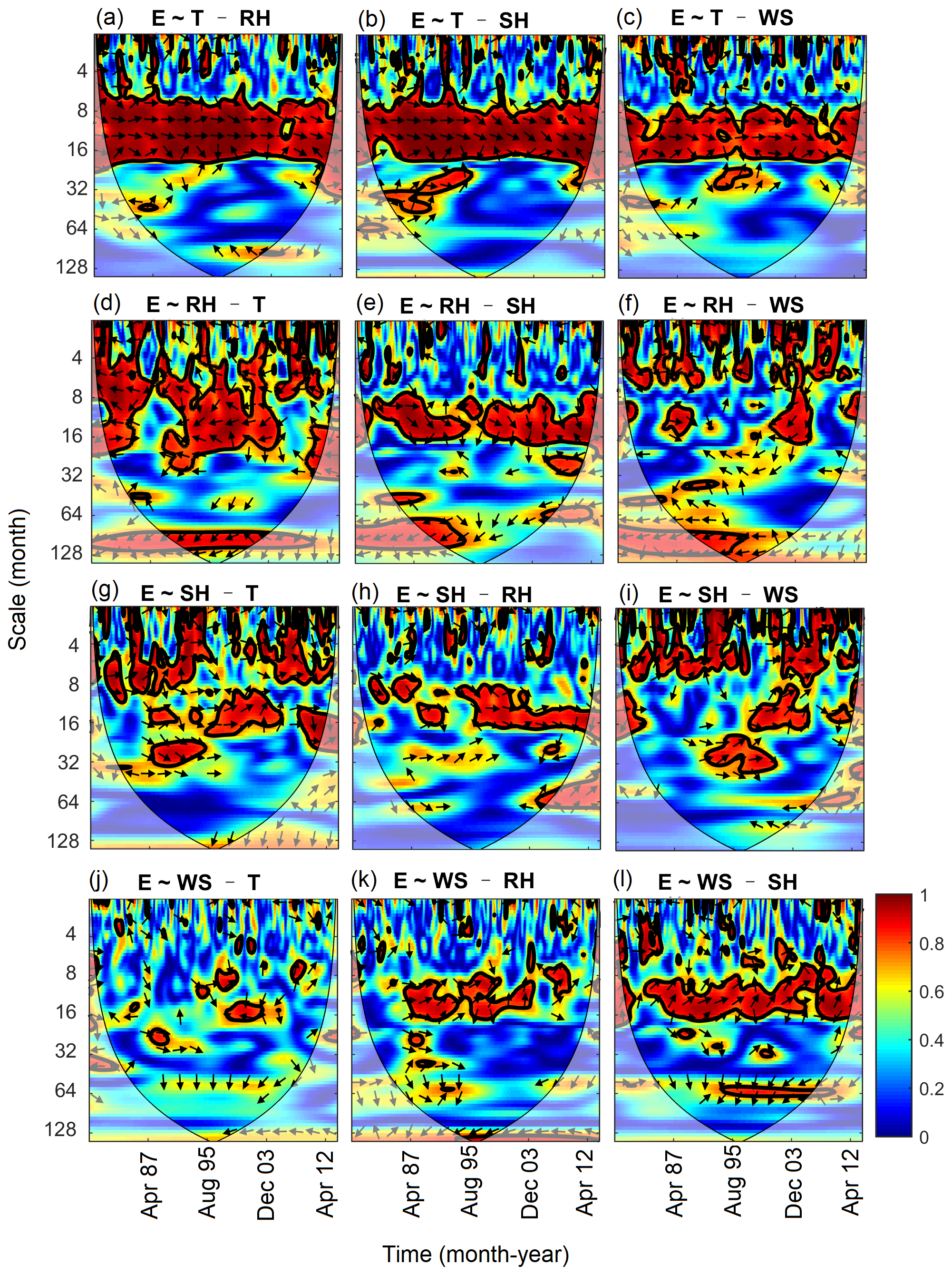
Figure 3 PWC between evaporation (E) and each meteorological factor (T, mean temperature; RH, relative humidity; SH, sun hours; WS, wind speed) after excluding the effect of each of the other three meteorological factors.

PWC between E and RH depended on the excluding variable and scale (Fig. 3d–f). The mean PWC and PASC between E and RH after excluding T were 0.60 and 34 %, respectively, which are comparable with the mean BWC (0.62) and PASC (40 %) between E and RH. The corresponding values after excluding SH and WS were 0.50 and 0.53 (PWC) and 22 % and 21 % (PASC), respectively. In addition, compared with the BWC between E and RH (Fig. S4 of Sect. S3), correlations between E and RH were weak at small scales (<8 months) and medium scales (8–32 months) after eliminating the influence of SH and WS (Fig. 3e–f), respectively. Therefore, excluding the variable of T had less influence on the coherence between E and RH compared with excluding the variables of SH and WS. This is mainly because RH and T are correlated with E at different scales (Fig. S4 of Sect. S3), i.e., mean temperature affected E mainly at medium scales, while RH affected E across all scales. However, the domain where SH and WS were correlated with E was a subset of that where RH and E were correlated (Fig. S4 of Sect. S3).

The relationships between E and SH after excluding the other three factors were less consistent (Fig. 3g–h). The areas with significant corrections were scattered over the whole location–scale domain but differed with excluding factor. The PASC varied from 12 % (excluding RH) to 20 % (excluding T and WS), which is much lower than the PASC (28 %) in the case of BWC. The significant relationships between E and WS were only limited to very small areas except for the case of SH being excluded, where E and WS were positively correlated at scales of 8–16 months most of the time (Fig. 3j–l).

In general, PASC decreased after excluding the effects of more factors (data not shown). The correlations between E and each variable after eliminating the effects of all other variables are shown in Fig. 4. The correlations between E and T were still significant at the medium scales (8–32 months) (Fig. 4a), where PASC value was 52 % with a mean PWC_sig of 0.92. The E was still correlated with RH at large scales (>85 months) (Fig. 4b), where PASC value was 35 % with a mean PWC_sig of 0.96. Interestingly, the domain with significant correlation between E and SH and WS was very limited (Fig. 4c–d). This indicates that the influences of SH and WS on E have already been covered by RH and T. This is in agreement with the MWC results that RH and T were best for explaining E variations at all scales (Hu and Si, 2016). Although the RH had the greatest mean wavelet coherence and PASC in the entire location–scale domains, the PWC analysis seems to support mean temperature being the most dominating factor for free water evaporation at the 1-year cycle (8–16 months), which is the dominant scale of E variation (Fig. S3 of Sect. S3).

Figure 4 PWC between evaporation (E) and each meteorological factor (T, mean temperature; RH, relative humidity; SH, sun hours; WS, wind speed) after excluding the effects of all three other factors.

5 Discussion on the advantages and weaknesses of the new method

5.1 Advantages

We extend the partial coherence method from the frequency (scale) domain (Koopmans, 1974) to the time–frequency (location–scale) domain. The new method is an extension of previous work on PWC and MWC (Mihanoviæ et al., 2009; Hu and Si, 2016). The method test and application have verified that it has the advantage of dealing with more than one excluding variable and providing the phase information associated with PWC. In the case of one excluding variable, Mihanoviæ et al. (2009) have suggested calculating PWC by using an equation analogous to the traditional partial correlation squared (Eq. 14), which can be derived from our Eq. (9). However, their equation was, unfortunately, widely used by replacing the complex coherence in Eq. (14) with real coherence as expressed in Eq. (15) (Ng and Chan, 2012b, a; Rathinasamy et al., 2017; Aloui et al., 2018; Altarturi et al., 2018; Jia et al., 2018; Li et al., 2018; Mutascu and Sokic, 2020; Wu et al., 2020). This mistake is corrected in this paper.

The differences between the new (Eq. 14) and classical (Eq. 15) implementations are compared in the case of one excluding variable using both the artificial and real datasets. Except for the phase information, the two implementations generally produce comparable coherence for the artificial dataset (Fig. S5 of Sect. S3 in the Supplement). However, the new implementation produces consistently and slightly higher coherence than the classical implementation. For example, their mean PWCs between y and y₂ at the scale of 8 after excluding the effect of y₄ are 1.00 and 0.97, respectively. This indicates that the new implementation produces coherence between y and y₂ at the scale (i.e., 8) of y₂, closer to 1 as we expect. While the classical implementation produces similar PWC between E and other meteorological factors in most cases, especially for the coherence between E and T after excluding the effects of others (Fig. S6 of Sect. S3 in the Supplement), large differences between these two implementations can also be observed. For example, while the new implementation recognizes the strong coherence between E and RH after excluding the effect of T at scales of around 1 year (Fig. 3d), this coherence was negligible by the classical implementation (Fig. 5a). Mean PWC values by the new implementation were consistently higher than the classical implementation, and the differences ranged from 0.4 to 0.6 around the scale of 1 year (Fig. 5b). Considering the real coherence (Eq. 15) rather than complex coherence (Eq. 14) between every two variables in the numerators can potentially result in large underestimation of the partial wavelet coherence. Therefore, the ability of the new method and implementation to produce more accurate results than the classical implementation is one of its advantages.

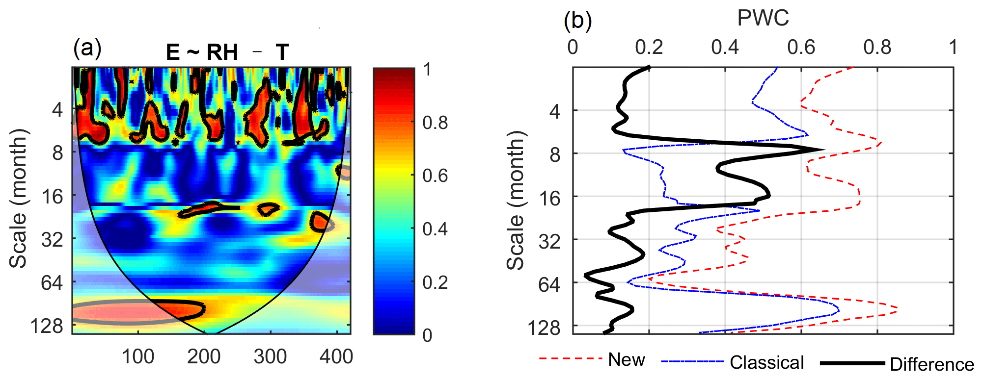
Figure 5 PWC between evaporation (E) and relative humidity (RH) after excluding the effect of mean temperature (T) using the classical implementation (Eq. 15) (a) and differences in PWC between the new (Eq. 14) and classical implementations as a function of scale (b).

Compared with the Mihanoviæ et al. (2009) method, the additional phase information from the new PWC is another advantage of this new method. This is because phase information is directly related to the type of correlation, i.e., in-phase and out-of-phase indicating positive and negative correlation, respectively. Different types of correlations were usually found at different locations and scales (Hu et al., 2017b). The phase information helps understand the differences in associated mechanisms or processes at different locations and scales. In addition, the phase information will allow us to detect the changes in not only the degree of correlation (i.e., coherence), but also the type of correlation after excluding the effect of other variables. For example, E and RH were positively correlated at the 1-year cycle (8–16 months) from years 1979 to 1995. This is because higher evaporation usually occurs in summer when high T coincides with high RH as influenced by the monsoon climate in the study area (Fig. S4 of Sect. S3). Interestingly, after excluding the effect of T, E was negatively correlated with RH at the scale of 1 year as we expect (Fig. 3d).

Moreover, our new PWC method applies to cases with more than one excluding variable, which is a knowledge gap. When multiple variables are correlated with both the predictor and response variables, the correlations between predictor and response variables may be misleading if the effects of all these multiple variables were not removed. For example, at the dominant scale (i.e., 1 year) of E variation, contrasting effects of RH on E existed after excluding the effects of T (negative) or SH (positive) (Fig. 3d and e). However, after the effects of all other variables were excluded, there were negligible effects of RH on E at this scale (Fig. 4b). In this case, the relationship between E and RH at the scale of 1 year can be misleading after removing the effects of only one variable. In addition, the dominant role of mean temperature in driving free water evaporation at the 1-year cycle was proved by removing the effects of all other meteorological factors (Fig. 4a). This also further verifies the suitability of the Hargreaves model (only air temperature and incident solar radiation required) (Hargreaves, 1989) for estimating potential evapotranspiration on the Chinese Loess Plateau (Li, 2012).

5.2 Weaknesses

The new method has the risk of producing spurious high correlations after excluding the effect from other variables. Take the artificial dataset for example: at the scale of 32, PWC values between y and y₂ after excluding y₄ are not significant but relatively high, partly because of small octaves per scale (octave refers to the scaled distance between two scales, with one scale being twice or half of the other, default of 1/12). This spurious unexpected high PWC is caused by low values in both the numerator (partly associated with the low coherence between response y and predictor variables y₂ at the scale of 32) and denominator (partly associated with the high coherence between response y and excluding variable y₄ at the scale of 32) in Eq. (9). The same problem also exists in the classical implementation (Fig. S5 of Sect. S3). So, caution should be taken to interpret those results. However, it seems that the domain with spurious correlation calculated by the new method is very limited, and it is located mainly outside of the cones of influence. Moreover, the unexpected results can be easily ruled out with knowledge of BWC between response and predictor variables. It is expected that the correlation between two variables should not increase after excluding one or more variables. Therefore, BWC analysis is suggested for better interpretation of the PWC results.

Similar to BWC and MWC, the confidence level of PWC calculated from the Monte Carlo simulation is based on a single hypothesis testing, but in reality, the confidence level of PWC values at all locations and scales needs to be tested simultaneously. Therefore, the significance test has the problem of multiple testing; i.e., more than one individual hypothesis is tested simultaneously (Schaefli et al., 2007; Schulte et al., 2015). The new method may benefit from a better statistical significance testing method. Options for multiple testing can be the Bonferroni adjusted p test (Westfall and Young, 1993) or false discovery rate (Abramovich and Benjamini, 1996; Shen et al., 2002), which is less stringent than the former. The AR(1) model was used to generate noise series for testing the confidence level of PWC. High-order autoregressive models rather than AR(1) may be beneficial for a significance test where spatial data (or time series) are characterized by long-range dependence (Szolgayová et al., 2014).

6 Conclusions

Partial wavelet coherency (PWC) is improved to investigate scale-specific and localized bivariate relationships after excluding the effect of one or more variables in geoscience. Method tests using stationary and non-stationary artificial datasets verified the known scale and localized bivariate relationships after eliminating the effects of other variables. Compared with the previous PWC method, the new PWC method has the advantage of dealing with more than one excluding variable and providing the phase information (i.e., correlation type) associated with PWC. In the case of one excluding variable, the PWC implementation provided here (in the paper and the published code) produces more accurate coherence than the previously published PWC implementation that considered wrongly real coherence rather than complex coherence between every two variables. Application of the new method to the real dataset has further proved its robustness in untangling the bivariate relationships after removing the effects of all other variables in multiple location–scale domains. The new method provides a much needed data-driven tool for unraveling underlying mechanisms in both temporal and spatial data. Thus, combined with wavelet transform, BWC, and MWC, the new PWC method can be used to analyze various processes in geoscience, such as streamflow, droughts, greenhouse gas emissions (e.g., N₂O, CO₂, and CH₄), atmospheric circulation, and oceanic processes (e.g., El Niño–Southern Oscillation).