the Creative Commons Attribution 4.0 License.
the Creative Commons Attribution 4.0 License.
 | 31 May 2021
Variations in surface roughness of heterogeneous surfaces in the Nagqu area of the Tibetan Plateau
Maoshan Li
Xiaoran Liu
Lei Shu
Shucheng Yin
Lingzhi Wang
Wei Fu
Yaoming Ma
Yaoxian Yang
Fanglin Sun
Temporal and spatial variations of the surface aerodynamic roughness lengths (Z0 m) in the Nagqu area of the northern Tibetan Plateau were analysed in 2008, 2010 and 2012 using MODIS satellite data and in situ atmospheric turbulence observations. Surface aerodynamic roughness lengths were calculated from turbulent observations by a single-height ultrasonic anemometer and retrieved by the Massman model. The results showed that Z0 m has an apparent characteristic of seasonal variation. From February to August, Z0 m increased with snow ablation and vegetation growth, and the maximum value reached 4–5 cm at the BJ site. From September to February, Z0 m gradually decreased and reached its minimum values of about 1–2 cm. Snowfall in abnormal years was the main reason for the significantly lower Z0 m compared with that in normal conditions. The underlying surface can be divided into four categories according to the different values of Z0 m: snow and ice, sparse grassland, lush grassland and town. Among them, lush grassland and sparse grassland accounted for 62.49 % and 33.74 %, and they have an annual variation of Z0 m between 1–4 and 2–6 cm, respectively. The two methods were positively correlated, and the retrieved values were lower than the measured results due to the heterogeneity of the underlying surface. These results are substituted into the Noah-MP (multi-parameterisation) model to replace the original parameter design numerical simulation experiment. After replacing the model surface roughness, the sensible heat flux and latent heat flux were simulated with a better diurnal dynamics.
- Article
(12273 KB) - Full-text XML
- BibTeX
- EndNote


Known as the “third pole” of Earth (Jane, 2008), the Tibetan Plateau (TP) has an average altitude of over 4000 m and accounts for a quarter of China's territory. It is located in southwestern China adjacent to the subtropical tropics in the south, and it reaches the mid-latitudes in the north, making it the highest plateau in the world. Due to its special geographical location and geomorphic characteristics, it plays an important role in the global climate system as well as the formation, outbreak, duration and intensity of the Asian monsoon (Yang and Yao, 1998; Zhang and Wu, 1998; Wu and Zhang, 1998, 1999; Wu et al., 2004, 2005; Ye and Wu, 1998; Tao et al., 1998). Many studies (Wu et al., 2013; Wang, 1999; Ma et al., 2002) have shown that the land–atmosphere interaction on the TP plays an important role in the regional and global climate. Over the past 47 years, the Tibetan Plateau has shown a significant warming trend and increased precipitation (Li et al., 2010). The thermal effects of the Tibetan Plateau not only have an important impact on the Asian monsoon and precipitation variability but also affect the atmospheric circulation and climate in North America, Europe and the southern Indian Ocean by inducing large-scale teleconnections similar to the Asian–Pacific Oscillation (Zhou et al., 2009).
The various thermal and dynamic effects of the Tibetan Plateau on the atmosphere affect the free atmosphere via the atmospheric boundary layer. Therefore, it is particularly important to analyse the micrometeorological characteristics of the atmospheric boundary layer of the Tibetan Plateau, especially the near-surface layer (Li et al., 2000). Affected by the unique underlying surface conditions of the Tibetan Plateau, local heating shows interannual and interdecadal variability (Zhou et al., 2009). Different underlying surfaces have differing diversities, complex compositions and uneven distributions, which also makes the land surface that they constitute diverse and has a certain degree of complexity. As the main input factor for atmospheric energy, the surface greatly affects the various interactions between the ground and the atmosphere and even plays a key role in local areas or specific times (Guan et al., 2009). The surface characteristic parameters (dynamic roughness, thermodynamic roughness, etc.) play an important role in the land surface process and are important factors in causing climate change (Jia et al., 2000). The underlying surface of the Tibetan Plateau presents different degrees of fluctuation, which introduces certain obstacles to understanding the land–atmosphere interaction of the Tibetan Plateau. The fluctuating surface may alter the arrangement of roughness elements on the surface and cause changes in surface roughness. Changes in roughness can also affect changes in the characteristics of other surface turbulent transportation, which may also result in changes in surface fluxes. Chen et al. (2015) presented a practical approach for determining the aerodynamic roughness length at fine temporal and spatial resolutions over the landscape by combining remote-sensing and ground measurements. Surface roughness is an important parameter in land surface models and climate models. Its size controls the exchange, transmission intensity and interactions between the near-surface airflow and the underlying surface to some extent (Liu et al., 2007; Irannejad and Shao, 1998; Shao, 2000; Zhang and Lv, 2003). Zhou et al. (2012) demonstrated that simulated sensible heat flux compared with measurement was significantly improved using a time-dependent Z0 m parameter. Therefore, the primary objective of this study is to calculate the surface roughness and its variation characteristics to further understand the land–atmosphere interactions on the central Tibetan Plateau.
Through the study of surface roughness, it is beneficial to obtain the land surface characteristics in the region, provide the ground truth value for model inputs, improve land surface simulations in the Tibetan Plateau and deepen the understanding of land–atmosphere interaction processes. Simulation of surface fluxes has made considerable progress in recent years, especially in the improvement of parameterisation schemes (Smirnova et al., 2016). Luo et al. (2009) used the land surface model CoLM to conduct a single-point numerical simulation at the BJ station and successfully simulated the energy exchange process in the Nagqu area. Zhang et al. (2017) evaluated the surface physical process parameterisation schemes of the Noah LSM (land surface model) and Noah-MP (multi-parameterisation) model in the entire East Asia region and evaluated the simulation of the surface heat flux of the Tibetan Plateau. Xie et al. (2017) explored the simulation effect of the land surface model CLM4.5 in the alpine meadow area of the Qinghai-Tibet Plateau. Xu et al. (2018) studied the applicability of different parameterisation schemes in the Weather Research and Forecasting (WRF) model when simulating boundary layer characteristics in the Nagqu area. Comparative analyses have been performed of the meteorological elements simulated by different land surface process schemes in the WRF model in the Yellow River source region (Zhang et al., 2020). However, the applicability of the model in the Tibetan Plateau needs further study. The terrain of the Tibetan Plateau is complex, the underlying surface is very uneven and the area has high spatial heterogeneity. Because the condition of the underlying surface has a very significant impact on the surface flux, obtaining information on the surface vegetation status of a certain area is very helpful for analysing the spatial representation of the surface flux.
In this study, satellite data were obtained by MODerate-resolution Imaging Spectroradiometer (MODIS), and the normalised difference vegetation index (NDVI) in the Nagqu area was used to study the dynamic surface roughness length. Atmospheric turbulence observation data in 2008, 2010 and 2012 and observation data from automatic weather stations were collected at three observation stations. The measured values of the average wind speed and turbulent flux of a single-height ultrasonic anemometer were used to determine the surface dynamic roughness Z0 m (Chen et al., 1993). The timescale dynamics of Z0 m and the results of different underlying surfaces were analysed. Through a comparison of the calculation results to the observation data, we studied whether the surface roughness values retrieved by satellites were reliable to provide accurate surface characteristic parameters. Then we used the retrieved surface roughness to replace the surface roughness in the original model for numerical simulation experiments, and evaluated the model simulation results. This research will be helpful for the study of land–atmosphere interactions in the plateau area and improvement of the theoretical research of the near-surface layer on the Tibetan Plateau. In the following section, we describe the case study area, the MODIS remote-sensing data, the ground observations and the land cover map used to drive the revised Massman model (Massman, 1997; Massman and Weil, 1999). In Sect. 3, we present the results and then a validation based on flux measurements at Nagqu station. Finally, we provide some concluding remarks on the variation characteristics of aerodynamic roughness lengths and numerical simulation of the surface turbulent flux in the Nagqu area of the central Tibetan Plateau.
2.1 Study area and data
The area selected in this study is a 200×200 km2 area centred on the Nagqu Station of Plateau Climate and Environment of the Northwest Institute of Ecology and Environmental Resources, Chinese Academy of Sciences.
In this area, three meteorological observatory stations are located: North Pam (Portable Automated Meso-net) Automatic Meteorological Observatory (NPAM), Nam Co Station for Multisphere Observation and Research, Chinese Academy of Sciences (NAMC) and BJ station (Fig. 1). The underlying surface around the observation site is relatively flat on a small spatial scale, and a certain undulation is observed at a large spatial scale. The data used included observations from atmospheric turbulence and automatic meteorological stations.
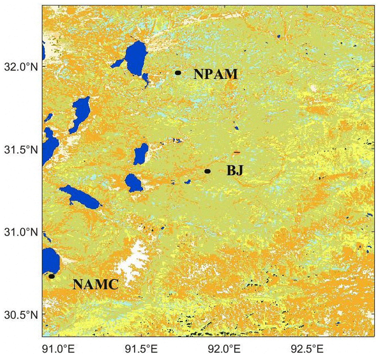
Figure 1Location of sites and the land cover on the northern Tibetan Plateau. The black solid circle “•” indicates the location of the sites.
The BJ station is located at coordinates 31.37∘ N, 91.90∘ E and has an altitude of 4509 m a.s.l. The BJ observation site is located in the seasonal frozen soil area, and the vegetation is alpine grassland. The site measurement equipment includes an ultrasonic anemometer (CAST3, Campbell, Inc.), infrared open path analyser (LI 7500), and an automatic meteorological observation system (Ma et al., 2006). This study uses the BJ station data from 2008 and 2012. The NPAM station is located at 31∘56′ N, 91∘43′ E and has an altitude of approximately 4700 m. The ground of the experimental field is flat, and the area is wide. The ground is covered by a plateau meadow that grows 15 cm high in summer. The experimental station observation equipment includes an ultrasonic wind thermometer and humidity probe pulsator and includes data on temperature and humidity, air pressure, average wind speed, average wind direction, surface radiative temperature, soil heat flux, soil moisture and temperature and radiation (Ma et al., 2006). The NAMC station is located at 30∘46.44′ N, 90∘59.31′ E and has an altitude of 4730 m. It is located on the southeastern shore of Nam Co lake in Namuqin Township, Dangxiong County, Tibet Autonomous Region. It is backed by the Nyainqêntanglha mountain range, and the underlying surface is an alpine meadow. This study uses NPAM station data for the whole year of 2012 and NAMC station data for the whole year of 2010.
The land cover data used in this study are GLC2009 (Arino et al., 2010) data from the Envisat satellite in 2009, and the spatial resolution is 300 m. The classification standard is the land cover classification system (LCCS), and it divides the global surface into 23 different types, with the study area including 14 of these types. The actual situation in the selected area does not match the data part of GLC2009 because of the lack of an underlying surface, such as farmland, in the selected area. Therefore, according to the actual land cover types obtained by Chu et al. (2010), the categories irrigated farmland, dry farmland, mixed farmland vegetation, mixed multi-vegetation land, closed grassland and open grassland are replaced with six grasslands, shrub meadows, mountain meadows, alpine grasslands, alpine meadows and sparse vegetation in the mountains. Since the proportion of the underlying surface of the tree as a whole is only 0.36 %, the underlying surface types evergreen coniferous forest, mixed forest, multi-forest grassland mix and multi-grass forestland mix will no longer be studied.
The MODerate-resolution Imaging Spectroradiometer (MODIS) is a sensor on board the satellites TERRA and AQUA launched by the US Earth Observing System Program. The band of the MODIS sensor covers the full spectrum from visible light to thermal infrared; thus, this sensor can detect surface and atmospheric conditions, such as surface temperature, surface vegetation cover, atmospheric precipitation and cloud top temperature. The finest spatial resolution is 250 m. The normalised vegetation index obtained by MODIS is the MYD13Q1 product, which provides a global resolution of 250 m per 16 d. This study selects 73 data files for 2008, 2010 and 2012 in Nagqu.
2.2 Methodology
2.2.1 Method for calculating surface roughness by observation data
Using the measured values of the average wind speed and turbulent flux of a single-height ultrasonic anemometer, the calculation scheme of surface roughness proposed by Chen et al. (1993) was selected, and the dynamic variation in the surface roughness was obtained.
According to the Monin–Obukhov similarity theory (Monin and Obhukov, 1954), the wind profile formula with the stratification stability correction function (Panosky and Dutton, 1984) is as follows:
where ; Z0 m is the dynamic surface roughness length; z is the height of wind observation; d is zero plane displacement, (Stanhill, 1969), h is the vegetation height. h takes 0 in winter, 0.020 in spring, 0.0450 in summer and 0.030 in autumn in this study; U is the average wind speed; k is the Karman constant, which is set to 0.40 (Högström, 1996); is the Monin–Obukhov length (Monin and Obhukov, 1954); ; and is the atmospheric stability parameter. Available from Eq. (1),
Using Eq. (2)–(4), Z0 m can be determined by fitting ζ and observing a single height .
2.2.2 Method for calculating surface roughness by satellite data
For a fully covered uniform canopy, Brutsaert (1982) suggested that Z0 m=0.13hv. For a canopy with proportional coverage (partial coverage), Raupach (1994) indicated that Z0 m varies with the leaf area index (LAI). However, Pierce et al. (1992) pointed out that for all kinds of biological groups, the leaf area index can be obtained from the NDVI, and the fractional cover of vegetation can be related to the NDVI. Asrar et al. (1992) pointed out that a mutual relationship occurred among the LAI, NDVI and ground cover through the study of physical models. The study by Moran et al. (1994) provides another method that uses the function of the relationship between NDVI and Z0 m in the growing season of alfalfa.
Considering that the main underlying surface of the study area is grassland, this study selects the Massman model (Massman, 1997; Massman and Weil, 1999). to calculate the Z0 m in the Nagqu area of the central Tibetan Plateau. The Massman model is calculated as follows:
where C1=0.32, C2=0.26 and C3=15.1 are constants in the model and related to the surface drag coefficient; LAI is the leaf area index; Cd=0.2 is the drag coefficient of the foliage elements; nec is the wind speed profile coefficient of fluctuation in the vegetation canopy; and h is the vegetation height. In many earlier studies, the high-altitude environment of the Tibetan Plateau was correlated with a low temperature in the study area and shown to affect the height and sparseness of the vegetation. Based on previous research, this study considers that the vegetation height in northern Tibet is related to the normalised difference vegetation index (NDVI) and altitude (Chen et al., 2013) and introduces the altitude correction factor on the original basis. The following is the calculation formula:
where hmin and hmax are the minimum and maximum vegetation height observed at the observation station, respectively, NDVImax and NDVImin are the maximum and minimum NDVI of the observation station, respectively; H is based on the assumption that the vegetation height is directly proportional to the NDVI; x is the altitude, which is obtained from ASTER's digital elevation model (DEM) products; and acf is the altitude correction factor (Chen et al., 2013), which is used to characterise the effect of elevation on the height of vegetation in northern Tibet. The acf parameter has the following form:
The LAI used in this study is calculated by the NDVI of MODIS (Su, 1996). The calculation formula is as follows:
3.1 Variation characteristics of surface roughness based on measured data
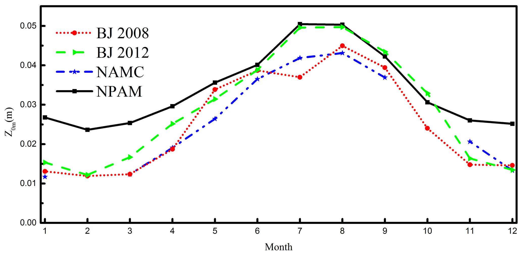
Figure 2 shows the temporal variation characteristics of the surface roughness of sites in different years in the Nagqu area. The Z0 m value has continued to increase since February to reach a maximum in July and August. The results for the BJ and NPAM stations in 2012 show that July has slightly larger ones than August, and the results for the NAMC station in 2010 and BJ station in 2008 show that August has larger values than July. After August, the Z0 m value began to decrease, and in December, the value was approximately the same as the value in January. In general, the change in the Z0 m degree of each station increases from spring to summer and decreases month by month from summer to winter.
3.2 Spatio-temporal variation characteristics of surface roughness length retrieved by MODIS data
Figure 3 shows a plot of the surface roughness distribution of 200×200 km2 around the BJ site in 2008. In February, the Z0 m decreased from January, which may have been due to snowfall or temperature, etc., resulting in a small Z0 m that continued to decrease. Due to the rising temperature and snow melting, Z0 m showed a slowly increasing trend from February to May and a rapid increase from June to August. From June onwards, a large number of surface textures were observed, indicating the complexity of the underlying surface. Whether the bulk surface or vegetation had a more important impact on Z0 m is not clear. From May to August, obvious changes in humidity, temperature and pressure caused by the plateau summer monsoon led to an increase in the height and coverage of surface vegetation, and Z0 m peaked in August. In particular, the change from May to June was very significant, which may have been related to the beginning of the summer monsoon in June, the corresponding increase in precipitation that accelerated the growth of vegetation and the rapid rise of Z0 m. In June, July and August, continuous precipitation and rising temperatures led to vigorous vegetation growth, although changes were not observed after the vegetation reached maturity. The corresponding maximum value of Z0 m in the figure remains unchanged, although due to high values in these 3 months, the area with high Z0 m values gradually expanded and reached the maximum range in August. From September to December, as the plateau summer monsoon retreated, the temperature and humidity gradually decreased. Compared with the plateau summer monsoon, the conditions were no longer suitable for vegetation growth; thus, the contribution of vegetation to Z0 m was weakened, the surface vegetation height gradually decreased and Z0 m continued to decrease. Moreover, the area with high Z0 m value also gradually decreased.
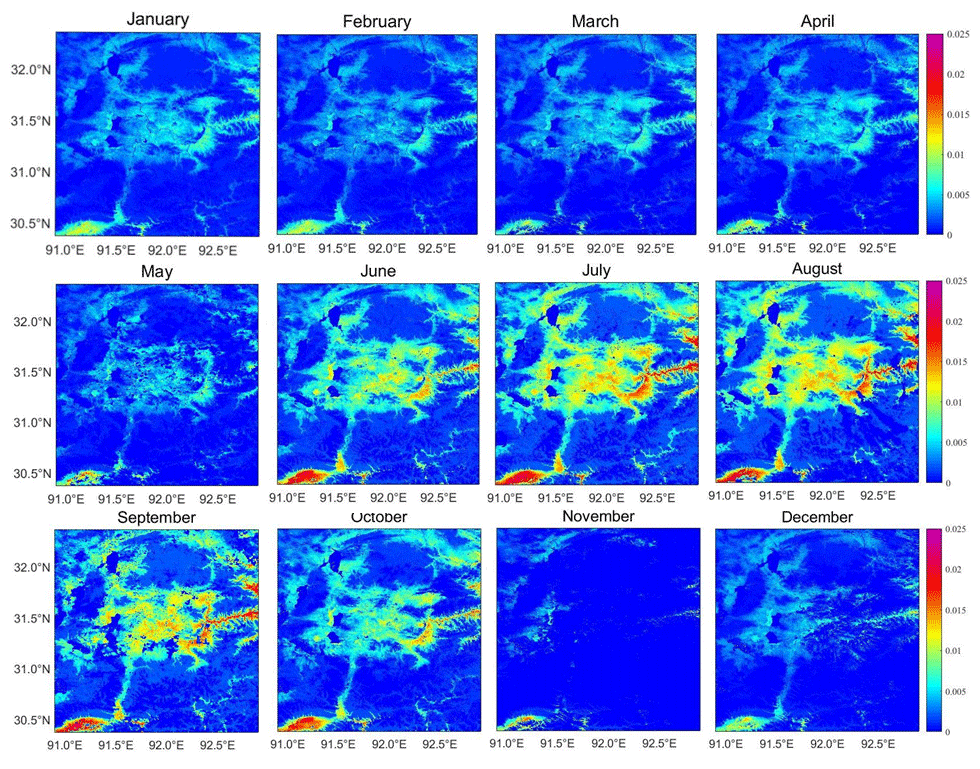
Figure 3Surface roughness length on the northern Tibetan Plateau in 2008.
Figures 4 and 5 show the retrieved monthly surface roughness values in the BJ area in 2010 and 2012, respectively. Moreover, Z0 m also showed a decrease from January to February in the Nagqu area in 2010 and 2012. Starting in February, Z0 m increased. Starting in June, Z0 m increased rapidly and reached the peak of the whole year in August. Subsequently, Z0 m began to decrease.
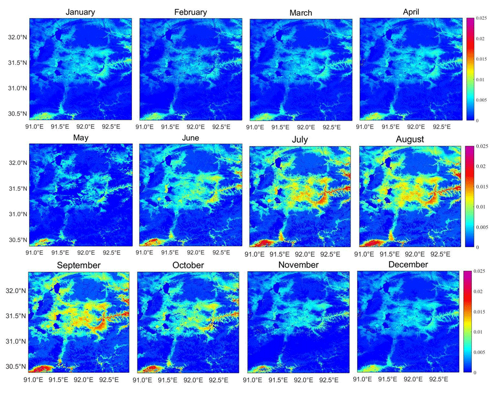
Figure 4Surface roughness length on the northern Tibetan Plateau in 2010.
Figures 3–5 show that Z0 m changes with the spatial and temporal scale. Z0 m shows different trends on different underlying surfaces. In November 2008, the Z0 m in the Nagqu area was small overall and generally as low as 1 cm. Historical data show that there is a large-scale snowfall process in the Nagqu area at this time. Snowfall over the meadow causes the underlying surface of the meadow to be homogeneous and flat, and after the snowfall falls, it is easy to form a block with a scattered and discontinuous underlying surface. We subsequently determined that the surface roughness of the area with ice and snow as the underlying surface is not more than 1 cm, which is consistent with historical weather processes. Therefore, we think that snowfall caused the Z0 m in November to be very small. From November to December, Z0 m showed a growing trend, which may be due to temperature, unfrozen soil or other reasons that resulted in the melting of snow, and then the surface roughness showed a growing trend (Zhou et al., 2017).
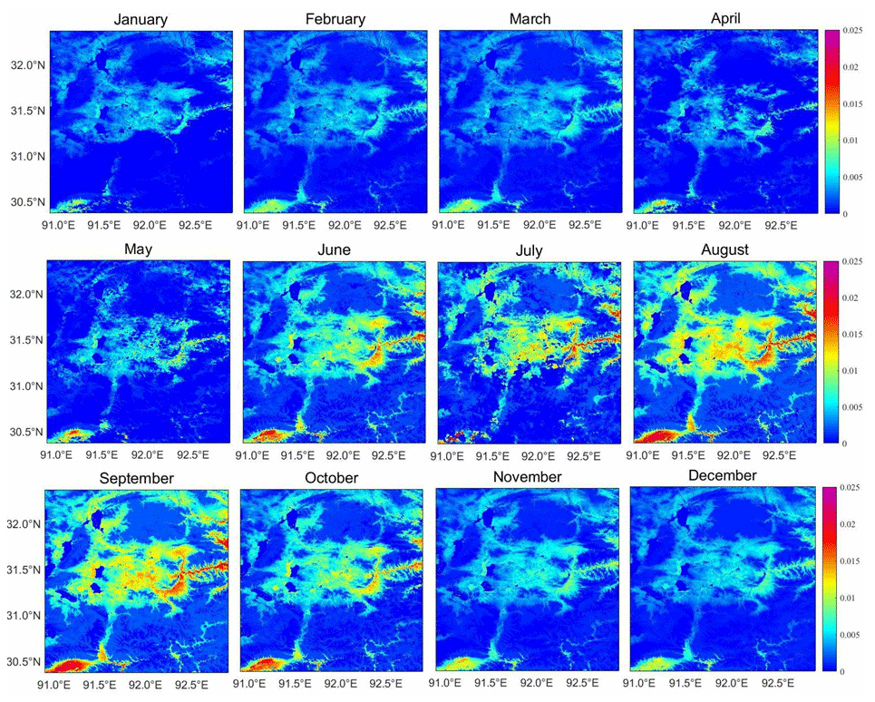
Figure 5Surface roughness length on the northern Tibetan Plateau in 2012.
3.3 Evaluation of satellite-data-retrieved results
The underlying surfaces of the three sites selected in this study are all alpine meadows. In Fig. 6, the NPAM site data calculation results are larger than the satellite-data-retrieved results throughout the year. Only the values in September and October are very close, and the trends are similar. The maximum value of the site data calculation is 5 cm, and the satellite-data-retrieved result is 4.5 cm. The maximum difference is in May at 1.7 cm. The NAMC station data calculation results are very close to the satellite-data-retrieved results from April to November, although the satellite-data-retrieved results are significantly larger than the site data calculation results in January, March and December. The largest difference occurs in January, and the difference value reaches 1.5 cm. In 2008, the calculation results of the BJ station data were larger than the satellite-data-retrieved results throughout the year. The calculation results of the site data were very close to the satellite-data-retrieved results from January to April and July to November, although a large difference was observed in May, June and December, with the largest difference occurring in May at 1.8 cm. In 2012, the BJ site data calculation results were consistent with the satellite-data-retrieved results for the whole year, although the site data calculation results were larger than the satellite-data-retrieved results from March to June, and the station data calculation results were smaller than the satellite-data-retrieved at other times. As a result, the largest difference occurred in June at 1.1 cm. Figure 6 shows that for the overall situation, the seasonal variation trend of the site data calculation results is consistent with the satellite-data-retrieved results in January, February, March, November and December. However, the site data calculation results from April to October are greater than the satellite-data-retrieved results. From Fig. 6, the Z0 m calculated from the site observation data is larger than that of the satellite data, which may be because of the average smoothing effect. From February to July, the single-point Z0 m value was significantly increased according to the independent method of determining the surface roughness, while the results obtained using the satellite data did not increase significantly. The satellite results show that the values from January to May, November and December are basically stable below 2 cm and only change from June to October, which is related to non-uniformity of the underlying surface in Massman model. In general, the results calculated by the station are generally larger than those obtained by satellite retrieval.

Figure 6Comparison of the surface roughness length by site observations and satellite-remote-sensing-retrieved data.
The Z0 m scatter plot is shown in Fig. 7. A significant positive correlation is observed between the satellite retrieval and the surface roughness calculated from the site data. The correlation coefficients between the observation result and the retrieved result are large, except for at the NAMC station in 2010 in Fig. 7g. The average results of the underlying surface were consistent with the underlying surface results in different regions, further indicating that the satellite-retrieved results are consistent with the site calculation results. However, the results of the NAMC site are different from those of the other sites. The correlation coefficient with the average results of the underlying surface is 0.83, and the correlation coefficient with the satellite-retrieved results is 0.62. Because the NAMC observation station is closer to the lake (1 km), it is more affected by local microclimates, such as lake and land winds. The results in Fig. 7 all passed the F test of P=0.05, which indicates that there is no significant difference between the site data calculation results and the satellite-data-retrieved results.
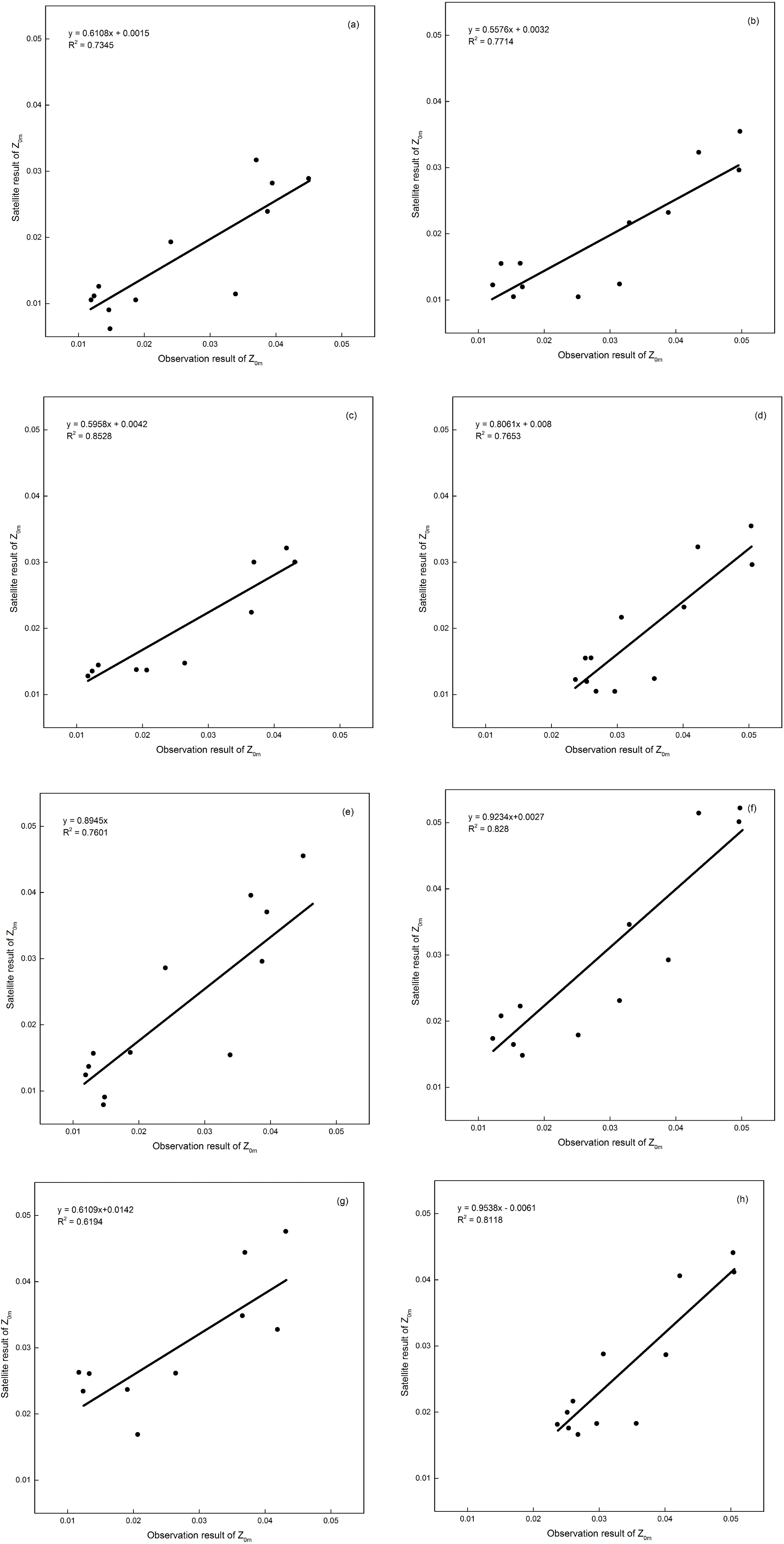
Figure 7Scatter plots of the retrieved and calculated surface roughness lengths at four sites.
According to the vegetation dataset GLC2009, combined with actual local conditions, the 200×200 km2 area of Nagqu was divided into 10 different underlying surfaces (Arino et al., 2010): mountain grassland, shrub meadow, mountain meadow, alpine grasslands, alpine meadows, sparse vegetation lap, urban land, bare land, water bodies, ice sheets and snow cover.
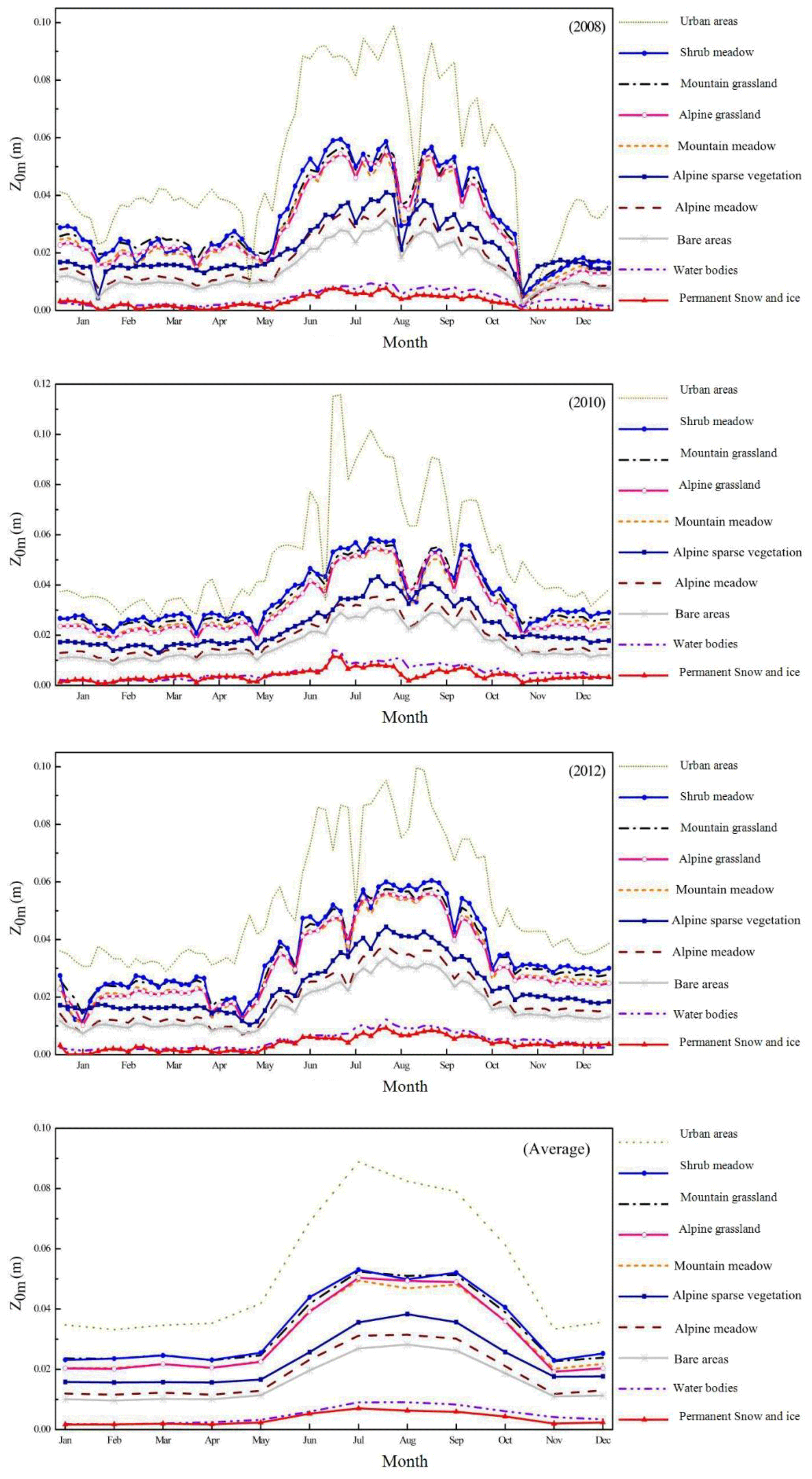
The monthly variation in Z0 m in different underlying surfaces in the Nagqu area is shown in Fig. 8, which indicates that 14 different underlying surfaces (Table 1) in the Nagqu area can be divided into four categories. The first category is urban land, which accounts for 0.07 % of the whole study area. The Z0 m of this type of underlying surface is greater than that of other types throughout the year, and the change in Z0 m is very large, which is probably due to the irregular changes in the underground areas of the selected areas and the irregularities caused by human activities. The second category is lush grassland, including shrub meadows, mountain grasslands, alpine grasslands and mountain meadows, which accounts for 62.49 % of the area. The variation curves of Z0 m of the four underlying surfaces are similar, and the Z0 m of the urban land is only smaller than that of other underlying surfaces. The third category is sparse grassland, including alpine sparse vegetation, alpine meadows and bare land, and it accounts for 33.74 % of the area. The Z0 m values of the three underlying surfaces are similar at a medium height. The Z0 m of the bare soil is at the lowest point of these underlying surface Z0 m, and the Z0 m of the alpine meadow is relatively stable and less affected by the outside vegetation. The fourth category is ice and snow, including ice surfaces and snow cover and water bodies, which are two kinds of underlying surfaces, accounting for 3.7 % of the area. The Z0 m of these three underlying surfaces presents another phenomenon. The variation range of the whole year is relatively small, and the Z0 m of these underlying surfaces is also small. It is more than 1 cm in mid-June and less than 1 cm at other times. Figure 8d shows the multi-year average seasonal variation in Z0 m. The figure clearly shows that the underlying surface can be divided into four categories due to the difference in surface roughness. The change from January to May Z0 m is very small, peaking from May to August and then down to the previous January to May level in November and December. The snowfall in November 2008 may have led to the low level of November in Fig. 8d. Table 2 shows that the winter albedo at the BJ station and NAMC station is higher than that in other seasons, and it is the smallest in the summer. The surface albedo at both stations in November 2008 was significantly higher than that in November of the other 2 years. In fact, the surface roughness in November should be higher than that in December in former years.
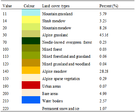
Table 2The observed albedo of the sites (BJ and NAMC) on the northern Tibetan Plateau.
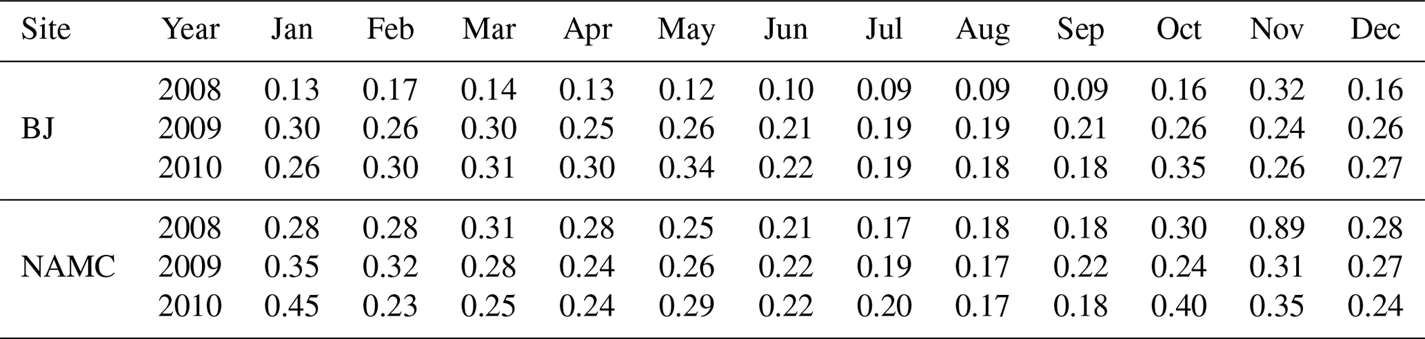
Figure 8 also shows that in the Nagqu area, except for the area of the fourth type of underlying surface, the Z0 m change in other areas decreases from January to February and begins to increase after February, reaching a peak in August and then starting to decrease. However, Fig. 6 clearly shows that there are several stages in which Z0 m changes significantly, in early April, mid-May, early July, late August and late September. The change at the end of August was the most obvious. At each of the underlying surfaces, Z0 m changes by more than 2 cm on average. The extent of the change in late September was also large, with an average change of more than 1.5 cm. Moreover, the change in early July was special because the change resulted in a significant increase in the Z0 m of water bodies and ice.
Certain factors, such as cloud cover in May, August and November 2008, August and September 2010, and April and July 2012, caused significant changes in the overall Z0 m, which resulted in two very significant changes in the 3-year average for August and November. In November, the change was caused by snowfall based on other meteorological data. In August 2008 and 2010, the changes were caused by precipitation based on an analysis of the sudden increase in the Z0 m of the water body and ice and snow surface. Combined with several changes in Z0 m, precipitation, snowfall and snow accumulation will make the underlying surface more uniform and flatter, which will lead to relative reductions in Z0 m.
5.1 Model setup
According to the surface roughness variation characteristics retrieved from satellite data, the underlying surface of Nagqu area can be divided into four types. They are urban, lush grass, sparse grass and ice and snow. Among them, urban accounts for 0.07 %, and its Z0 m is up to 9 cm; lush grassland accounts for 62.49 % of the area, and its Z0 m can reach up to 6 cm; sparse grassland accounts for up to 33.74 %, and its Z0 m can reach up to about 4 cm; and ice and snow accounts for 3.7 % of the area, and the Z0 m does not exceed 1 cm. These results are substituted into Noah-MP to replace the original parameter design numerical simulation experiment. The model after replacing the surface roughness is set as a sensitivity experiment, and the original model is set as a control experiment. The selection of other parameterisation schemes suitable for numerical simulation in the Nagqu area is shown in Table 3. The simulation time is from 1 to 31 July 2008, and the spin-up time is 9 d. The forcing field dataset is a Chinese meteorological forcing dataset (He et al., 2020), jointly developed by the Tibetan Plateau Data Assimilation and Modelling Centre and the Institute of Tibetan Plateau Research of the Chinese Academy of Sciences (ITPCAS).
5.2 Evaluation of the simulated single-point heat flux
Figure 9a shows that the sensible heat flux simulated by the sensitivity experiment is closer to the measured value than the control experiment at the BJ site. In the daytime, the results of sensitivity experiment were in general smaller than those of the control experiment. At night, the results of the two models were close to each other before 21 July, and the sensitivity experiment results were significantly improved after 21 July. Figure 9b shows that the sensitivity experiment results are basically consistent with the control experiment results at the BJ site, which are maintained at about 0 W m−2, and there is no improvement at night. Before 19 July, the latent hear fluxes for the two experiments remained at about 200 W m−2, which was less than the observed latent heat flux, and the simulated maximum value of the sensitivity experiment was greater than that of the control experiment. After 19 July, the two experiments simulation results began to increase and reached about 400 W m−2, consistent with the observed latent heat flux, indicating that the simulation effect was improved to some extent. Similarly, it can be found from the maximum value that the sensitivity experiment results were slightly greater than the control experiment results. The simulated values of sensible heat fluxes at NAMC and NPAM sites (Fig. 9c and e) are significantly larger than the observation results, but the sensitivity experiment results are better than the control experiments, while latent heat flux in the sensitivity experiment is greater than that in the control experiment and is close to the observation results at NPAM site (Fig. 9f). It also shows that improving the accuracy of surface roughness can improve the simulation effect of latent heat flux.
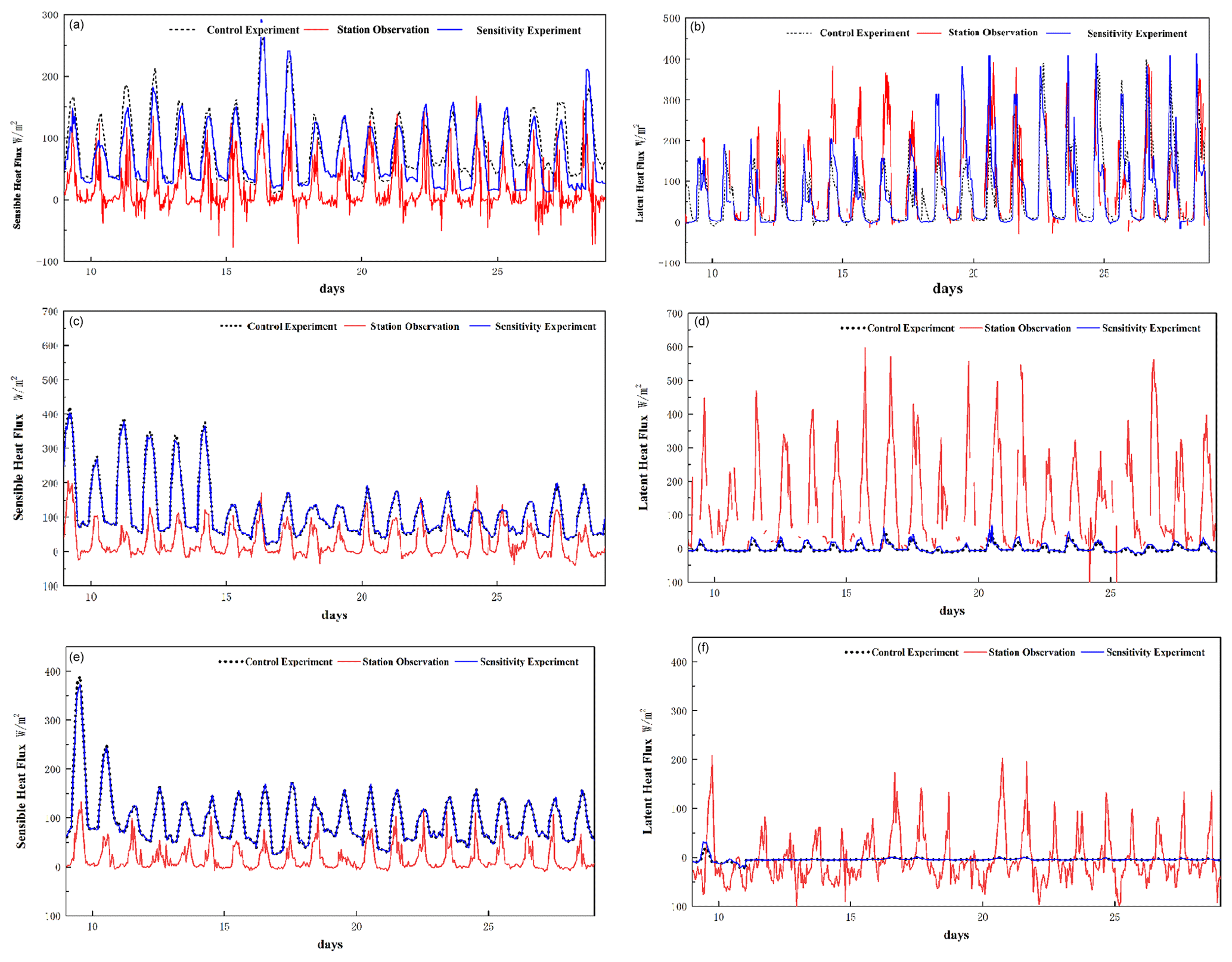
Figure 9Comparison of simulated and observed sensible heat flux (a, c, e) and latent heat flux (b, d, f) at BJ, NAMC and NPAM sites.
5.3 Evaluation of regional heat flux simulation results
In order to compare the changes of sensible heat flux and latent heat flux before and after improvement, the sensitivity simulations are used to subtract the control model simulation results. By subtracting the sensible heat flux of control from sensitivity experiment, the results are shown in Fig. 10. It can also be seen from Fig. 10a that the difference of sensible heat flux is basically negative in the daytime, indicating that the sensible heat flux after improvement is smaller than that before improvement. The above results show that the modified surface roughness can improve the simulation effect of sensible heat flux in daytime. The results in Fig. 10c are basically positive in the daytime, indicating that the latent heat flux after improvement is larger than that before improvement, about 15 W m−2. The above results show that the model simulation results are generally less than the actual observation results, so it can be considered that the improvement of surface roughness in the daytime can improve the simulation of heat fluxes. Figure 10 also shows that the improvement of night-time latent heat flux is not significant, which is basically maintained at 0 W m−2.
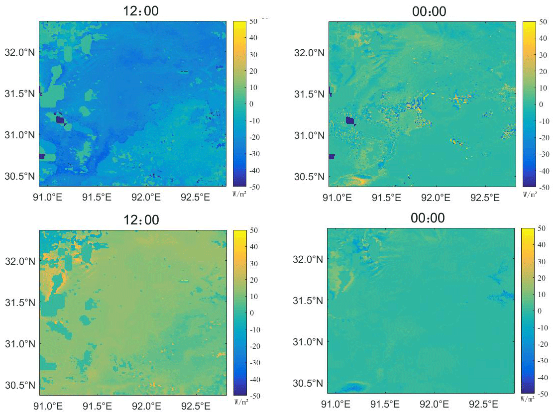
Figure 10The difference of the control and sensitivity experiments simulated regional sensible heat flux at (a) 12:00 LT and (b) 00:00 LT and latent heat flux at (c) 12:00 LT and (d) 00:00 LT.
Through the calculation and analysis of the surface roughness of the Nagqu area in the central Tibetan Plateau and comparing the retrieved satellite data with the calculation results of the observational data, the main conclusions attained are as follows.
-
The retrieved results of the satellite data are basically consistent with the calculated results of the measured data. Both results indicate that the surface roughness continued to increase from February to August, began to decrease after reaching a peak in August and reached the lowest value in February of the following year. A strong connection is observed between the monthly variation in surface roughness and the changes in meteorological elements brought by the plateau summer monsoon. Among them, the satellite surface retrieval results in a slow increase in surface roughness from February to May.
-
Through the characteristics of surface roughness variation retrieved by satellite data, the underlying surface can be divided into four categories according to the surface roughness (from large to small): urban, lush grassland, sparse grassland and ice and snow. Among them, lush grassland accounts for 62.49 %, and the Z0 m can reach 6 cm; sparse grassland accounts for 33.74 %, and the Z0 m can reach up to 4 cm; and ice and snow accounts for 3.7 %, and the Z0 m does not exceed 1 cm.
-
Comparing satellite-retrieved results and measured data shows that the results are positively correlated, and the satellite-retrieved results fit the measured results better. Due to the average sliding effect of the retrieved data, the satellite-retrieved data are smaller than the measured results. This method can be used to calculate the surface roughness results for a region and provide a true value for the model for simulation.
-
The accuracy of ground–air flux simulation can be improved after adjusting the surface roughness in the Nagqu area. After replacing the model surface roughness, the sensible heat flux has improved by 20 W m−2 during the daytime. The improvement for the simulation of sensible heat flux is poor at night, about 0.15 W m−2. The improvement of latent heat flux is not obvious, and there is an improvement within 15 W m−2 during the daytime.
This study uses remote-sensing images and an aerodynamic roughness remote-sensing-retrieved model to estimate the spatial scale of aerodynamic roughness conditions in northern Tibet, and this method will provide parameter and parameterisation scheme improvements for model simulations to study the spatial distribution of the surface flux in the Tibetan Plateau. Air thermodynamics surface roughness (Z0 h) is affected by shortwave and longwave radiation (the latter for deriving surface temperature), air temperature, wind speed, precipitation and snowfall. The relationship between air thermodynamics surface roughness and these other variables and how to parameterise them in the Massman model will be studied in the future.
The surface roughness length code used in this article is available online at https://doi.org/10.5281/zenodo.4797701 (Li and Liu, 2021).
The surface energy fluxes data used in this article are available online at https://doi.org/10.11888/Meteoro.tpdc.270910 (Ma, 2020).
ML, XL, LS and YY mainly wrote the manuscript and were responsible for the research design, data preparation and analysis. YM and ML supervised the research, including methodology development, as well as manuscript structure, writing and revision. ML drafted the manuscript. FS, SY, LW and WF prepared the data and wrote this paper.
The authors declare that they have no conflict of interest.
This article is part of the special issue “Data acquisition and modelling of hydrological, hydrogeological and ecohydrological processes in arid and semi-arid regions”. It is not associated with a conference.
This work was financially supported by the Second Tibetan Plateau Scientific Expedition and Research (STEP) program (grant no. 2019QZKK0103), the National Natural Science Foundation of China (grant nos. 41675106 and 41805009), the National Key Research and Development Program of China (grant no. 2017YFC1505702) and the Scientific Research Project of Chengdu University of Information Technology (grant no. KYTZ201721).
This research has been supported by the Second Tibetan Plateau Scientific Expedition and Research (STEP) program (grant no. 2019QZKK0103).
This paper was edited by Philip Brunner and reviewed by three anonymous referees.
Arino, O., Ramos, J., Kalogirou, V., Defourny, P., and Achard, F.: Glob Cover 2009, in: Proceedings of the living planet Symposium, Edinburgh, UK, 686–689, available at: http://hdl.handle.net/2078.1/74498 (last access: 18 February 2011), 2010.
Asrar, G., Myneni, R. B., and Choudhury, B. J. : Spatial heterogeneity in vegetation canopies and remote sensing of absorbed photosynthetically active radiation: A modelling study, Remote Sens. Environ., 41, 85–103, https://doi.org/10.1016/0034-4257(92)90070-Z, 1992.
Brutsaert, W. A.: Evaporation into the Atmosphere, D. Reidel Publishing Company, Dordrecht, the Netherlands, 113–121, https://doi.org/10.1007/978-94-017-1497-6, 1982.
Chen, J., Wang, J., and Mitsuaki, H.: An independent method to determine the surface roughness length, Chin. J. Atmos. Sci., 17, 21–26, https://doi.org/10.3878/j.issn.1006-9895.1993.01.03, 1993.
Chen, Q. T., Jia, L., Hutjes, R., and Menenti, M.: Estimation of Aerodynamic Roughness Length over Oasis in the Heihe River Basin by Utilizing Remote Sensing and Ground Data, Remote Sens., 7, 3690–3709, https://doi.org/10.3390/rs70403690, 2015.
Chen, X., Su, Z., Ma, Y., Yang, K., Wen, J., and Zhang, Y.: An improvement of roughness height parameterization of the Surface Energy Balance System (SEBS) over the Tibetan Plateau, J. Appl. Meteorol. Clim., 52, 607–622, https://doi.org/10.1175/JAMC-D-12-056.1, 2013.
Chu, D., Basabta, S., Wang, W., Zhang, Y. L., Liu, L. S., and Shushil, P.: Land Cover Mapping in the Tibet Plateau Using MODIS Imagery, Resour. Sci., 32, 2152–2159, 2010.
Guan, X. D., Huang, J. P., Guo, N., Bi, J. R., and Wang, G. Y.: Variability of soil moisture and its relationship with surface albedo and soil thermal parameters over the Loess Plateau, Adv. Atmos. Sci., 26, 692–700, https://doi.org/10.1007/s00376-009-8198-0, 2009.
He, J., Yang, K., Tang, W., Lu, H., Qin, J., and Chen, Y.: The first high-resolution meteorological forcing dataset for land process studies over China, Scient. Data, 7, 25, https://doi.org/10.1038/s41597-020-0369-y, 2020.
Högström, U.: Review of Some Characteristics of the Atmospheric Surface Layer, Bound.-Lay. Meteorol., 78, 215–246, https://doi.org/10.1007/BF00120937, 1996.
Irannejad, P. and Shao, Y. P.: Description and validation of the atmosphere-land-surface interaction scheme (ALSIS) with HAPEX and Cabauw data, Global Planet. Change, 19, 87–114, https://doi.org/10.1016/S0921-8181(98)00043-5, 1998.
Jane, Q.: The third pole, Nature, 454, 393–396, 2008.
Jia, L.: The Characteristics of Roughness Length for Heat and Its Influence on Determination of Sensible Heat Flux in Arid Zone, Plateau Meteorol., 19, 495–503, 2000.
Li, J. L., Hong, Z. X., and Sun, S. F.: An Observational Experiment on the Atmospheric Boundary Layer in Gerze Area of the Tibetan Plateau, Chin. J. Atmos. Sci., 24, 301–312, https://doi.org/10.1007/s10011-000-0335-3, 2000.
Li, L., Chen, X. G., Wang, Z. Y., Xu, W. X., and Tang, H. Y.: Climate Change and Its Regional Differences over the Tibetan Plateau, Adv. Clim. Change Res., 6, 181–186, https://doi.org/10.3969/j.issn.1673-1719.2010.03.005, 2010.
Li, M., and Liu, X.: code_for calculate z0m in Matlab, Zenodo, https://doi.org/10.5281/zenodo.4797701, 2021.
Liu, J., Zhou, M., and Hu, Y.: Discussion on the Terrain Aerodynamic Roughness, Ecol. Environ., 16, 1829–1836, 2007.
Luo, S., Lü, S., and Yu, Z.: Development and validation of the frozen soil parameterization scheme in Common Land Model, Cold Reg. Sci. Technol., 55, 130–140, 2009.
Ma, Y.: A long-term dataset of integrated land-atmosphere interaction observations on the Tibetan Plateau (2005–2016), National Tibetan Plateau Data Center, https://doi.org/10.11888/Meteoro.tpdc.270910, 2020.
Ma, Y. and Wang, J. M.: Analysis of Aerodynamic and Thermodynamic Parameters on the Grassy Marshland Surface of Tibetan Plateau, Prog. Nat. Sci., 12, 36–40, 2002.
Ma, Y., Tsukamoto, O., Wang, J. M., Ishikawa, H., and Tamagawa, I.: Analysis of aerodynamic and thermodynamic parameters on the grassy marshland surface of Tibetan Plateau, Prog. Nat. Sci., 12, 36–40, 2002.
Ma, Y., Yao, T., Wang, J., and Hu, Z.: The Study on the Land Surface Heat Fluxes over Heterogeneous Landscape of the Tibetan Plateau, Adv. Earth Sci., 21, 1215–1223, 2006.
Massman, W.: An analytical one-dimensional model of momentum transfer by vegetation of arbitrary structure, Bound.-Lay. Meteorol., 83, 407–421, https://doi.org/10.1023/A:1000234813011, 1997.
Massman, W. and Weil, J. C.: An analytical one-dimensional second-order closure model of turbulence statistics and the Lagrangian time scale within and above plant canopies of arbitrary structure, Bound.-Lay. Meteorol., 91, 81–107, https://doi.org/10.1023/A:1001810204560, 1999.
Monin, A. and Obukhov A.: Basic laws of turbulent mixing in the atmosphere near the ground, Tr. Akad. Nauk SSSR Geofiz. Inst., 24, 163–187, 1954.
Moran, M . S., Clarke, T. H., Inone, Y., and Vidal, A.: Estimating crop water deficit using the relation between surface-air temperature and spectral vegetation index, Remeot Sens. Environ., 49, 246–263, https://doi.org/10.1016/0034-4257(94)90020-5, 1994.
Panosky, H. A. and Dutton, J. A.: Atmospheric Turbulence: Models and Methods for Engineering Applications, John Wiley, New York, 1–399, 1984.
Pierce, L. L., Walker, J., and Downling, T. I.: Ecological change in the Murry-Darling Basin – III: A simulation of regional hydrological changes, J. Appl. Ecol., 30, 283–294, 1992.
Raupach, M. R.: Simplified expressions for vegetation roughness lengh and zero-plane displacement as functions of canopy height and area index, Bound.-Lay. Meteorol., 71, 211–216, 1994.
Shao, Y.: Phtsics and Modeling of Wind Erosion, Kluwer Academic Publishers, London, 1–452, 2000.
Smirnova, T. G., Brown, J. M., Benjamin, S. G., and Kenyon, J. S.: Modifications to the rapid update cycle land surface model (RUC LSM) available in the weather research and forecasting (WRF) model, Mon. Weather Rev., 144, 1851–1865, https://doi.org/10.1175/MWR-D-15-0198.1, 2016.
Stanhill, G.: A simple instrument for the field measurement of turbulent diffusion flux, J. Appl. Meteorol., 8, 509–513, 1969.
Su, Z.: Remote Sensing Applied to Hydrology: The Sauer River Basin Study, PhD Thesis, Wageningen University and Research, Wageningen, the Netherlands, 1996
Tao, S. Y., Chen, L. S., and Xu, X. D.: Progresses of the Theoretical Study in the Second Tibetan Plateau Experiment of Atmospheric Sciences (Part I), China Meteorological Press, Beijing, 1–348, 1998.
Wang, J.: Land Surface Process Experiments and Interaction Study in China – from HEIFE to Imgrass and GAME-TIBET/TIPEX, Plateau Meteorol., 18, 280–294, 1999.
Wu, G. and Zhang, Y.: Tibetan Plateau forcing and timing of the Mon-soon onset over south Asia and the south China sea, Mon. Weather Rev., 4, 913–927, 1998.
Wu, G. and Zhang, Y.: Thermal and Mechanical Forcing of the Tibetan Plateau and Asian Monsoon Onset Part: Timing of the Onset, Chin. J. Atmos. Sci., 23, 52–62, https://doi.org/10.1016/S0013-4686(02)00731-4, 1999.
Wu, G. X., Mao, J. Y., and Duan, A. M.: Recent progress in the study on the impact of Tibetan Plateau on Asian summer climate, Acta Meteorol. Sin., 62, 528–540, 2004.
Wu, G. X., Liu, Y. M., Liu, X., Duan, A. M., and Liang, X. Y.: How the heating over the Tibetan Plateau affects the Asian climate in summer, Chin. J. Atmos. Sci., 29, 47–56, https://doi.org/10.1360/gs050303, 2005.
Wu, X. M., Ma, W. Q., and Ma, Y. M.: Observation and Simulation Analyses on Characteristics of Land Surface Heat Flux in Noethern TibetanPlateau in Summer, Plateau Meteorol., 32, 1246–1252, 2013.
Xie, Z. P., Hu, Z. Y., Liu, H. L., Sun, G. H., Yang, Y., Lin, Y., and Huang, F. F.: Evaluation of the Surface Energy Exchange Simulations of Land Surface Model CLM4.5 in Alpine Meadow over the Qinghai-Xizang Plateau, Plateau Meteorol., 36, 1–12, 2017.
Xu, L. J., Liu, H. Z., Xu X. D., Du, Q., and Wang, L.: Applicability of WRF model to the simulation of atmospheric boundary layer in Nagqu area of Tibetan Plateau, Acta Meteorol. Sin., 76, 955–967, 2018.
Yang M. X., and Yao T. D.: A Review of the Study on the Impact of Snow Cover in the Tibetan Plateau on Asian Monsoon, J. Glaciol. Geocryl., 20, 90–95, 1998.
Ye, D. Z. and Wu, G. X.: The role of heat source of the Tibetan Plateau in the general circulation, Meteorol. Atmos. Phys., 67, 181–198, https://doi.org/10.1007/BF01277509, 1998.
Zhang, G., Zhou, G. S., and Chen, F.: Analysis of Parameter Sensitivity on Surface Heat Exchange in the Noah Land Surface Model at a Temperate Desert Steppe Site in China, Acta Meteorol. Sin., 31, 1167–1182, https://doi.org/10.1007/s13351-017-7050-1, 2017.
Zhang, Q. and Lv, S. H.: The Determination of Roughness Length over City Surface, Plateau Meteorol., 22, 24–32, 2003.
Zhang, Y., Yan, D., Wen, X., Li, D., Zheng, Z., Zhu, X., Wang, B., Wang, C., and Wang, L.: Comparative analysis of the meteorological elements simulated by different land surface process schemes in the WRF model in the Yellow River source region, Theor. Appl. Climatol., 139, 145–162, 2020.
Zhang, Y. S. and Wu, G. X.: Diasnostic Investigations of Mechanism of Onset of Asian Summer Monsoon and Abrupt Seasonal Transitions Over Northern Hemisphere PartI, Acta Meteorol. Sin., 56, 2–17, https://doi.org/10.11676/qxxb1998.047, 1998.
Zhou, X. J., Zhao, P., Chen, J. M., Chen, L. X., and Li, W. L.: Impacts of Thermodynamic Processes over the Tibetan Plateau on the Northern Hemispheric Climate, Sci. China Ser. D, 52, 1679–1693, https://doi.org/10.1007/s11430-009-0194-9, 2009.
Zhou, Y. L., Ju, W., Sun, X., Wen, X. F., and Guan, D.: Significant decrease of uncertainties in sensible heat flux simulation using temporally variable aerodynamic roughness in two typical forest ecosystems of China, J. Appl. Meteorol. Clim., 51, 1099–1110, https://doi.org/10.1175/JAMC-D-11-0243.1, 2012.
Zhou, Y., Xu, W., Bai, A., Zhang, J., Liu, X., and Ouyang, J. F.: Dynamic Snow-melting Process and its Relationship with Air Temperature in Tuotuohe, TibetanPlateau, Plateau Meteorol., 36, 24–32, 2017.
- Abstract
- Introduction
- Study area, data and methods
- Results analysis
- Variation characteristics of the surface roughness of different underlying surfaces
- Simulation and evaluation of the impact of surface roughness on turbulent fluxes using the Noah-MP model
- Conclusions and discussion
- Code availability
- Data availability
- Author contributions
- Competing interests
- Special issue statement
- Acknowledgements
- Financial support
- Review statement
- References