the Creative Commons Attribution 4.0 License.
the Creative Commons Attribution 4.0 License.
 | 25 May 2021
Advances in soil moisture retrieval from multispectral remote sensing using unoccupied aircraft systems and machine learning techniques
Anna Fryjoff-Hung
Andreas Anderson
Joshua H. Viers
Teamrat A. Ghezzehei
This study investigates the ability of machine learning models to retrieve the surface soil moisture of a grassland area from multispectral remote sensing carried out using an unoccupied aircraft system (UAS). In addition to multispectral images, we use terrain attributes derived from a digital elevation model and hydrological variables of precipitation and potential evapotranspiration as covariates to predict surface soil moisture. We tested four different machine learning algorithms and interrogated the models to rank the importance of different variables and to understand their relationship with surface soil moisture. All the machine learning algorithms we tested were able to predict soil moisture with good accuracy. The boosted regression tree algorithm was marginally the best, with a mean absolute error of 3.8 % volumetric moisture content. Variable importance analysis revealed that the four most important variables were precipitation, reflectance in the red wavelengths, potential evapotranspiration, and topographic position indices (TPI). Our results demonstrate that the dynamics of soil water status across heterogeneous terrain may be adequately described and predicted by UAS remote sensing and machine learning. Our modeling approach and the variable importance and relationships we have assessed in this study should be useful for management and environmental modeling tasks where spatially explicit soil moisture information is important.
- Article
(16080 KB) - Full-text XML
-
Supplement
(1226 KB) - BibTeX
- EndNote


The relatively small quantity of water stored in the upper layers of the soil plays a key role in terrestrial biology, biogeochemistry, and atmospheric water and energy fluxes. More than half of the solar energy absorbed by the land surface is used to evaporate water (Trenberth et al., 2009), and about 60 % of terrestrial precipitation is returned to the atmosphere by evapotranspiration (Seneviratne et al., 2010).
In most environments, soil water storage mainly depends on precipitation and evapotranspiration (Hillel, 1998; Rana and Katerji, 2000), but the distribution of water in the soil is also dependent on soil hydraulic properties, topography, and other environmental and belowground conditions (Korres et al., 2015; Vereecken et al., 2014; Western et al., 1999). Because of the complex interplay of these variables, it is a challenge to accurately estimate soil water. It is typically impractical to acquire data on soil water dynamics by direct measurement on scales larger than a small experimental plot, and there is no robust approach to predict it. The scarcity of soil moisture data is often cited as a major impediment for the investigation of soil moisture–climate interaction. Modern techniques for large-scale measurement of soil moisture include the cosmic-ray soil moisture observing system (COSMOS)- and the global positioning system interferometric reflectometry (GPS-IR)-based methods. The COSMOS employs a network of probes across the United States that estimate soil moisture by measuring cosmic-ray neutron radiation intensity above the land surface (Zreda et al., 2012). GPS-based methods are also able to estimate soil moisture of a few square meters using a GPS signal reflected from the soil. These techniques, while very promising, still need to be refined for routine use (Ochsner et al., 2013).
Remote sensing methods of retrieving soil moisture provide an alternative to conventional methods of soil moisture measurement, which are impractical at large scales. Several remote sensing methods, particularly from spaceborne deployment, have been developed to retrieve soil moisture using optical, thermal infrared, and microwave sensors. Remote sensing methods enable spatially distributed and frequent observations over a large area, which is difficult to achieve when using conventional field measurements (Barrett and Petropoulos, 2014; Petropoulos et al., 2015). A critical challenge to the current remote sensing methods of retrieving soil moisture is the lack of imagery with optimum spatial resolutions appropriate for field-scale soil moisture studies and the low revisit frequency of satellites (Barrett and Petropoulos, 2014; Das and Mohanty, 2006). Alternatives based on occupied airborne platforms are limited due to their high operational costs. Another persistent challenge to soil moisture remote sensing is the difficulty of estimating root zone soil moisture from the surface observations (Nichols et al., 2011; Ochsner et al., 2013).
Water is one of the most significant chromophores in soils, and studies have shown that narrow band spectral information in the visible (0.4–0.7 µm), near-infrared (0.7–1.1 µm), and shortwave infrared (1.1–2.5 µm) regions can be used to estimate surface soil moisture (Ben-Dor et al., 2009; Malley et al., 2004). Soil reflectance in the visible to shortwave infrared spectral region generally decreases with an increase in soil moisture, with some parts of the spectrum showing a more pronounced decrease than others (Haubrock et al., 2008; Weidong et al., 2002). The hydroxide bond is the strongest absorber in the near-infrared region, and free water in soil pores has strong absorption at around the 1.4 and 1.9 µm wavebands (Malley et al., 2004). Several hyperspectral techniques for estimating soil moisture content have been developed, such as the soil moisture Gaussian model (SMGM; Whiting et al., 2004) and the normalized soil moisture index (NSMI; Haubrock et al., 2008).
In the presence of vegetation cover, however, the ability to use soil reflectance to measure soil moisture is limited (Muller and Décamps, 2000). In addition, the reflectance of solar radiation from soil surface represents only about 50 µm of the upper soil. This makes it challenging to estimate the moisture conditions beneath thin surface layers (Malley et al., 2004). Most soil moisture remote sensing approaches operating in the optical range rely on developing an empirical spectral vegetation index (Barrett and Petropoulos, 2014). Several soil moisture measurement methods based on vegetation index proxies have been suggested as vegetation indexes are extremely sensitive to water stress, and they allow indirect estimates of soil moisture (Zhang and Zhou, 2016). Many studies have focused on deriving surface soil moisture content from the synergistic use of remote sensing data acquired simultaneously in the optical and thermal infrared spectrum. The so-called universal triangular relationship is a widely used method for estimating soil moisture (Nichols et al., 2011; Sobrino et al., 2014).
Retrieval of information from remote sensing measurements is based on the principle that changes in the chemical, physical, and/or structural characteristics of a target determine the variations in its electromagnetic response (Schanda, 1986). The task of retrieving information from remote sensing is complicated by several factors. Ali et al. (2015) summarize the retrieval challenges as being (i) the often complex and nonlinear relation between remote sensing measurement and target variables of interest; (ii) the ill-posed nature of the retrieval problem in that electromagnetic response of a target is typically the result of contributions from multiple target variables, and similar electromagnetic responses may be associated with different physical variables; (iii) the mixed contribution of multiple objects represented within elementary resolution cell; and (iv) the influence of external disturbing factors such as noise, radiation components coming from surrounding of the investigated area, and the atmosphere.
Soil moisture retrieval from remote sensing has traditionally been done by either empirical approaches or approaches based on an inversion of physical models. More recently, the use of machine learning techniques has gained increased attention because of their ability to tackle many of the limitations with the empirical approaches and physical-model-based approaches.
Physical-model-based approaches depend on an understanding of the mechanisms involving the interaction of electromagnetic radiation and the target variable. A wide variety of analytic electromagnetic models have been proposed in the literature. The thermal inertia approach (Price, 1977) is one such method that is most commonly used for soil moisture retrieval using thermal infrared (wavelengths between 3.5 and 14 µm) observation (Barrett and Petropoulos, 2014; Zhang and Zhou, 2016). Many new soil thermal inertia estimation methods continue to be developed (Price, 1985; Tian et al., 2015; Zhang and Zhou, 2016). The advantages of such physically based models are that they can operate in more general scenarios that are difficult to represent through the collection of in situ measurements. However, such models rely on simplifying the representation of a real phenomenon, which can reduce reliability. A major drawback of analytical models is their complexity and requirement for a large number of input parameters (Zhang and Zhou, 2016).
Empirical modeling approaches, on the other hand, employ statistical regression techniques to develop a mapping function based on in situ measurements of the target variable and corresponding remote sensing measurement. The advantage of empirical relationships is that they are typically fast to derive and require fewer inputs. However, such models require a higher-quality ground measurement, which could be time consuming and expensive, and the derived relationship is typically site and sensor dependent, which limits the possibility of extending their use readily in a different area (Ali et al., 2015).
Specific drawbacks to soil moisture remote sensing, using the optical and thermal infrared spectrum, are their shallow soil penetration ability and the cloud-free atmospheric condition requirement. Many of the optical and thermal infrared synergistic approaches require a wide range of both vegetation index and soil moisture conditions within a study region, which cannot always be satisfied (Barrett and Petropoulos, 2014).
The advantages of machine learning techniques in remote sensing are their ability to learn and approximate complex nonlinear mappings and the fact that no assumptions need to be made about data distribution. They can, thus, integrate data from different sources with poorly defined or unknown probability density functions and have often been shown to outperform other parametric approaches (Ali et al., 2015; Paloscia et al., 2008). Some of the limitations of machine learning methods are the need for a large number of training data, which require extensive ground truth data sets, and that machine learning methods are black boxes, and only limited inference can be made about the relationships of different inputs.
Remote sensing from unoccupied aircraft systems (UAS) has the potential to address several limitations of traditional remote sensing. The most attractive feature is their high spatial resolution, frequent or on-demand image acquisition, and low operating costs (Anderson and Gaston, 2013; Berni et al., 2009; Colomina and Molina, 2014; Elarab, 2016; Manfreda et al., 2018; Tmušić et al., 2020). UAS is an umbrella term that refers to the unoccupied aircraft and the complementary ground control and communication systems necessary for air surveys (Singh and Frazier, 2018).
1.1 Objectives
The purpose of this research was to advance soil moisture change measurement, process understanding, and prediction using remote sensing products from UAS and machine learning methods. In this study, the spatial and temporal scale limitations were addressed by deploying multispectral remote sensing with small UAS and surface soil moisture changes were retrieved using machine learning.
The specific goals of this study were as follows: (1) to develop an adaptable method for retrieving information on surface soil moisture from small UAS remote sensing products and machine learning methods, (2) to identify important reflectance and surface characteristics for the prediction of soil moisture changes, (3) to identify appropriate spatial resolutions of reflectance images and terrain variables for estimating soil moisture, and (4) to explore the relation of soil moisture with surface properties.
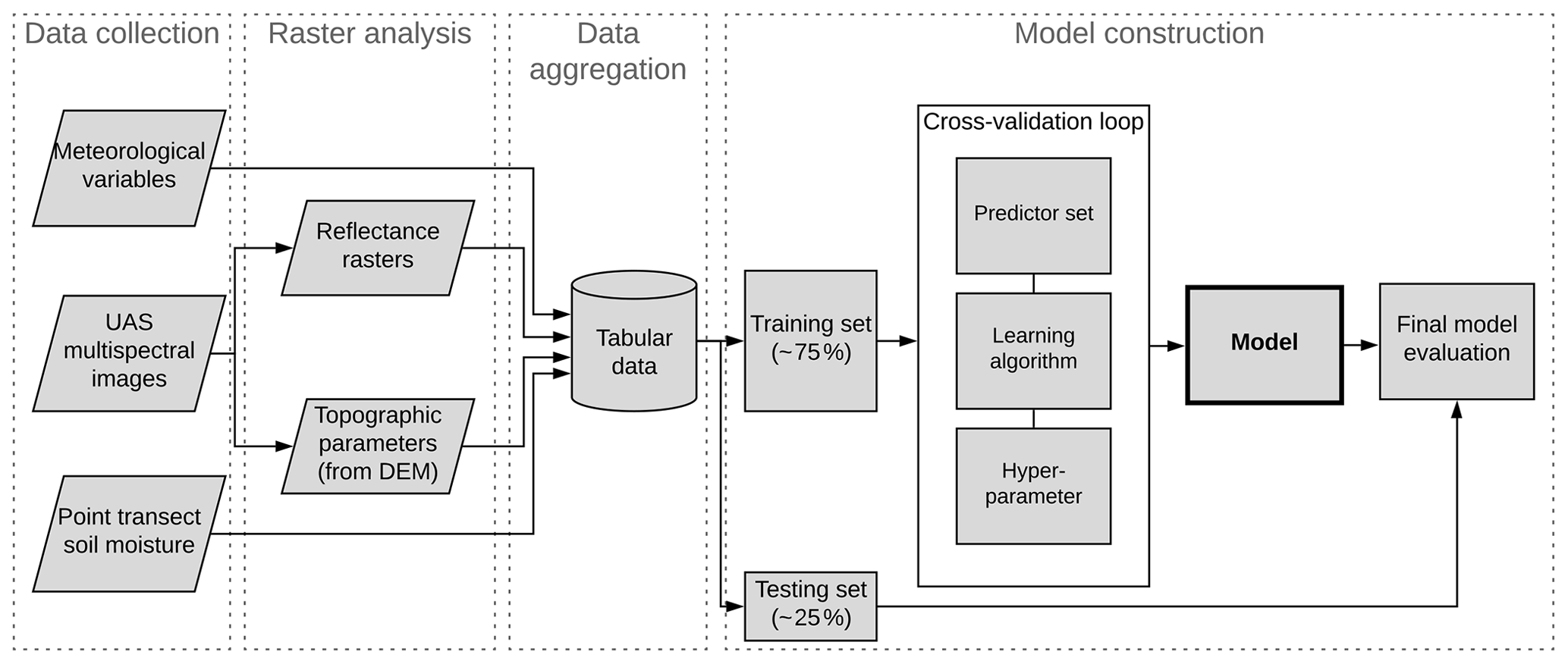
Multispectral images of the study area were collected on 6 different days throughout the 2018 water year using a UAS equipped with a multispectral camera. A high-resolution, centimeter-scale digital elevation model (DEM) was generated from the stereo images using photogrammetric software, and multiple sets of terrain variables were calculated. Concurrently with the image acquisition flights, the moisture content of the top 3.8 cm of soil was measured at predefined sampling locations. The ground soil moisture measurements, multispectral reflectance, terrain variables, and rainfall and potential evapotranspiration (PET) data were then aggregated into a data table and used to train a machine learning model to predict the soil moisture. Figure 1 shows the model building process.
2.1 Study site
The study was conducted in a small grassland catchment at the Merced Vernal Pools and Grassland Reserve located about 5 km northeast of the city of Merced, California. The grassland is used for livestock grazing; it has a Mediterranean climate with hot, dry summers and cool, wet winters, with an average annual precipitation of 330 mm (Wong, 2014).
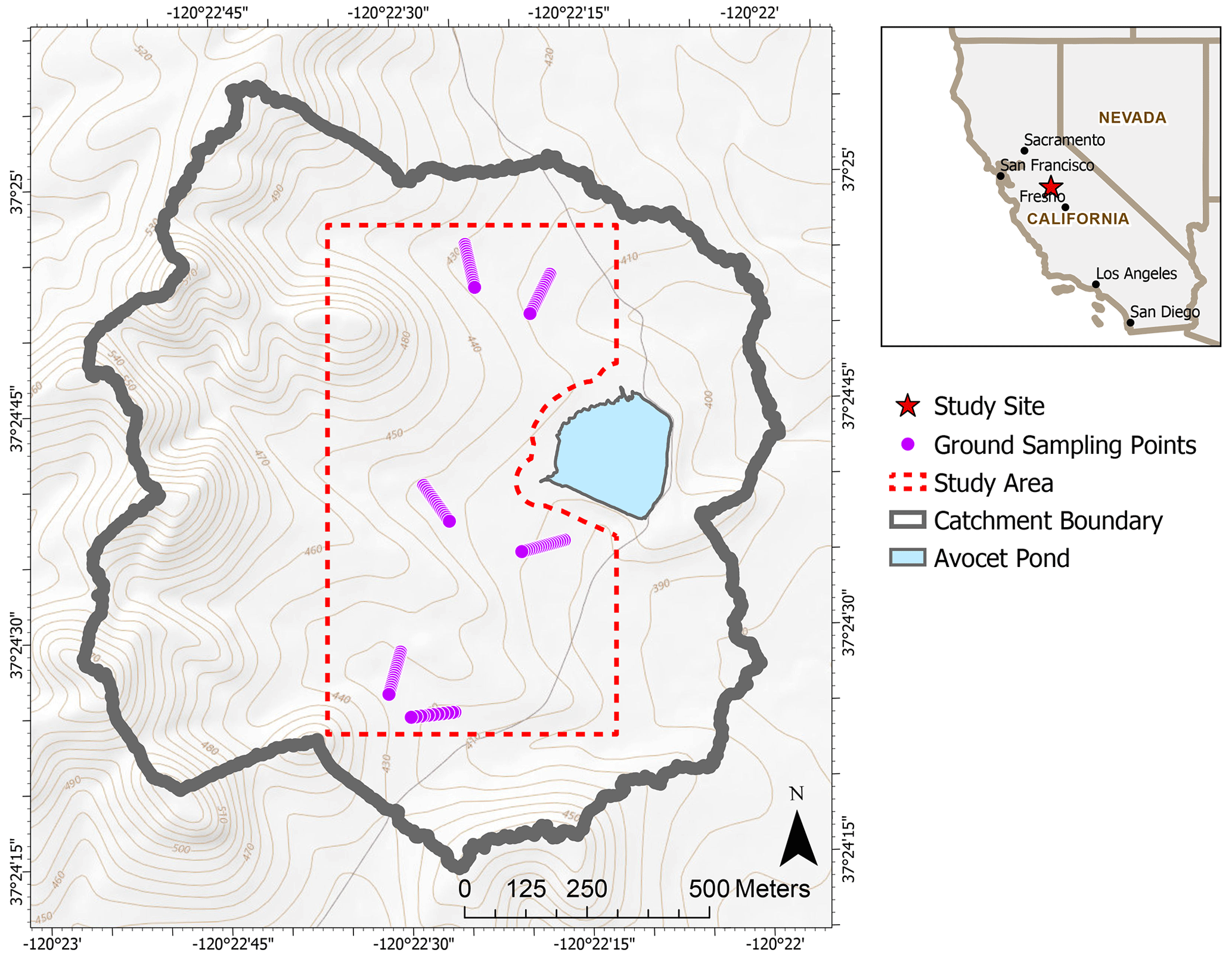
Figure 2Map of the Avocet Pond catchment showing the footprint of the study area, ground sampling points, and elevation contours in meters. Inset shows the location of the study site in California.
Our study site is a 0.6 km2 area of land located within a subcatchment that contributes to the Avocet Pond, a large stock pond located in the northeastern corner of the reserve (Fig. 2). The catchment was selected because of an extensive hydrologic modeling study that was being conducted on the site at the time (Fryjoff-Hung, 2018).
The study area soils are dominated by Redding gravelly loam (fine, mixed, active, thermic Abruptic Durixeralfs) soils. The elevation of the study area ranges from 118 to 162 m above sea level, and the slope ranges from 0 to 31∘. The distributions of elevation and slope are shown in Fig. S1 in the Supplement.

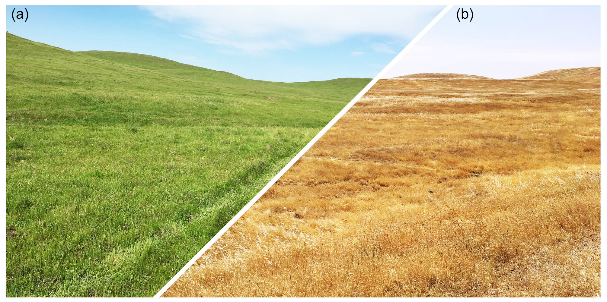
The vernal pool's ecology is predominantly controlled by large seasonal shifts and high spatial variability in hydrology; this makes the study site attractive for our study. UAS remote sensing has the potential to provide information at appropriate spatial and temporal scales for vernal pool studies (Stark et al., 2015). The annual seasonal cycle of the study site is shown in Fig. 3.
2.2 Data collection and preparation
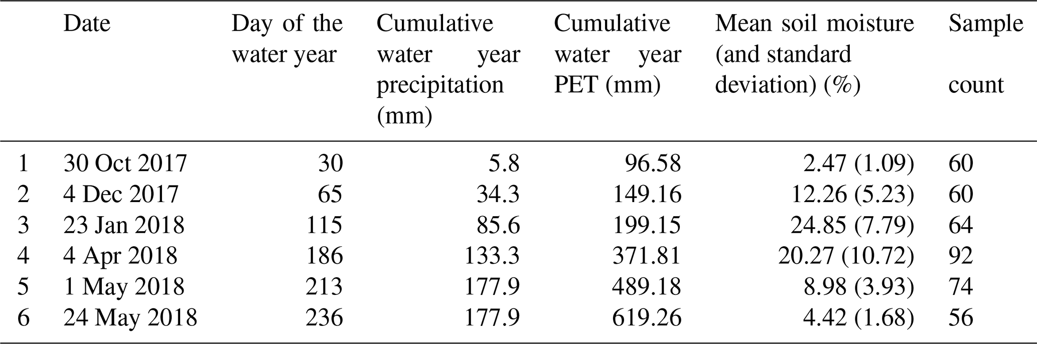
The imagery was acquired on 6 d during the 2018 water year green-up and brown-down, using a fixed-wing UAS with a multispectral camera onboard (see Table 3). Figure 4 shows a typical scene of the study site during the wet and dry seasons. Point soil moisture measurements (top 4 cm) were collected with a time domain reflectometry (TDR) probe across precise sampling transects identified with a real-time kinematic (RTK) positioning survey. Daily rainfall and PET values were acquired from nearby weather stations.
2.2.1 Image acquisition and processing
Multispectral images were acquired using a Parrot Sequoia sensor (Parrot SA, Paris, France) equipped with a sunshine sensor that measured irradiance at the sensor spectral wavebands for radiometric normalization. The camera is deployed on a fixed-wing unoccupied aircraft (Finwing Sabre; Finwing Technology) with an average flight height of 120 m above ground level. Images of a calibrated reflectance panel (MicaSense, Inc., Seattle, WA) were taken before each flight and used in the radiometric calibration of the images. The UAS remote sensing flights were conducted between late mornings and early afternoons during clear weather conditions. A single remote sensing–soil moisture collection campaign takes between 3 and 4 h. Images were acquired between 10:00 and 14:00 local time (LT).
The Parrot Sequoia sensor captures four separable bands in the green, red, red edge, and near-infrared bands, with a focal length of 3.98 mm and resolution of 1280 × 960 pixels. A fifth channel captures a high-resolution image in the visible spectrum, with a focal length of 4.88 mm and a resolution of 4608 × 3456. Images for the study area were captured with a minimum of 85 % overlap and a ground pixel resolution of 10 to 15 cm. Images were scaled to a uniform 15 cm pixel resolution during post-processing. Image processing was done using Pix4D photogrammetry software (Pix4D, Lausanne, Switzerland). A DEM was photogrammetrically generated from the overlapping stereo images, and images were orthorectified and radiometrically calibrated.
Geometric and radiometric corrections
Between seven and nine ground control point (GCP) targets, with precise locations identified by RTK survey, were used for photo alignment. The mean georeferencing root mean square errors (RMSEs) of the GCPs ranged from 0.6 to 2 cm, and the mean reprojection errors ranged from 0.1 to 0.2 px, based on the bundle block adjustment error assessment report. DEM was generated using the structure-from-motion technique; noise filtering and mild surface smoothing (sharp smoothing) were applied to correct for the noisy and erroneous points of the point cloud. The inverse distance weighting algorithm was used to interpolate between points to create the raster DEM.
Radiometric calibration by the Pix4D software considers the positional data, solar irradiance measurements, and gain and exposure data from the camera to convert raw digital numbers into sensor reflectance values. Sensor reflectance represents the ratio of the reflected light to the incoming solar radiation and provides a standardized measure that is directly comparable between images. Finally, surface reflectance is calculated in post-processing, taking into account the camera's orientation, the angle of the Sun, and the known reflectance values of the calibration panel.
2.2.2 In situ soil moisture measurement
The moisture content of the top 4 cm of soil was measured simultaneously with UAS remote sensing flights using a FieldScout TDR 300 soil moisture meter equipped with a 3.8 cm probe (Spectrum Technologies Inc., IL, USA). The FieldScout TDR 300 measures volumetric water content, using time domain reflectometry, with a resolution of 0.1 % and an accuracy of ± 3 %.
Accurate geolocation of the in situ soil moisture measurement points is critical for an overlay analysis of the ground measurements with remote sensing products. To ensure accurate geolocations of the ground measurements, we identified six 90 m long sampling transects and recorded the survey grade geolocation of the transect ends using the RTK positioning survey. The transect ends were marked with a metal peg hammered into the ground. During each soil moisture measurement campaign, a 90 m tape measure was temporarily affixed between the two ends of the transect, and soil moisture measurements were taken about every 10 m, noting the exact distance of the sampling point from the transect ends.
The sampling transects were laid out in a way that ensured that they run over a variety of topographic variables in terms of flow accumulation, topographic wetness index, and stream networks. Furthermore, each sampling transect fell in a separate subbasin within the Avocet basin.
2.2.3 Hydrological variables
Daily precipitation data were retrieved from the University of California, Merced, weather station located approximately 6 km southwest of the study site (California Department of Water Resources, 2018). Daily reference evapotranspiration data were retrieved from the California Irrigation Management Information System's (CIMIS) Merced station located approximately 10 km south of the study site (California Irrigation Management Information System, 2018). The reference evapotranspiration is evapotranspiration from standardized grass calculated using the modified Penman (CIMIS Penman) and Penman–Monteith equations (California Irrigation Management Information System, n.d.). In this study, we will refer to the reference evapotranspiration as the potential evapotranspiration (PET).
2.3 Data processing
To prepare the data for machine learning, we compiled all the information into a table with the measured soil moisture from each sampling point and date organized into one column. Each row contained the accompanying information for that sampling point and time.
Table 1Measured and calculated data used for machine learning. All topographic variables are computed from the digital elevation model. Descriptions and significance of topographic variables are adapted from Wilson and Gallant (2000).
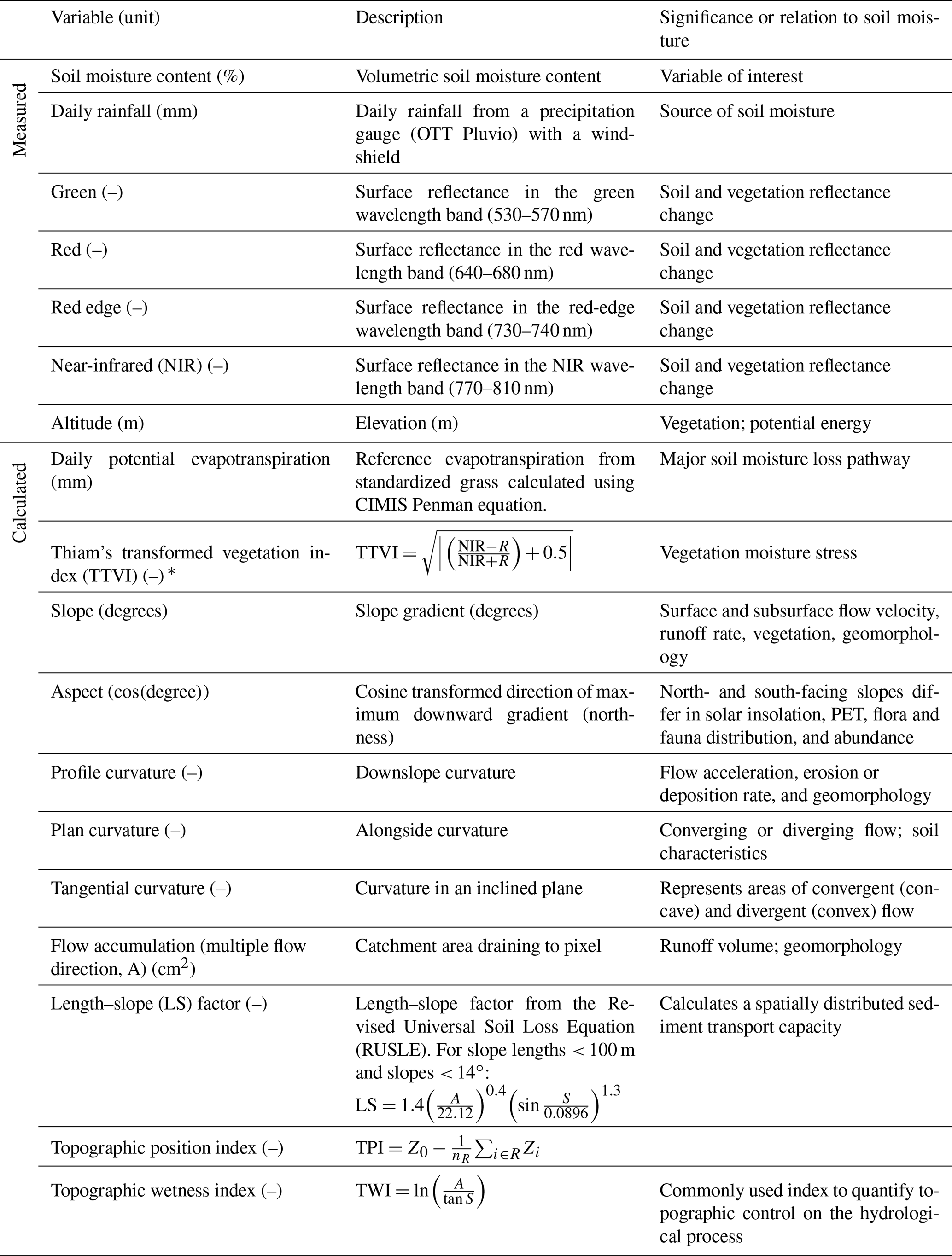
* The TTVI is a transformation of the commonly used normalized difference vegetation index (NDVI). The reason for choosing the TTVI transformation is that it eliminates negative values and often transforms NDVI histograms into a more normal distribution. Normalizing machine learning inputs is considered good practice and aids models in converging faster.
2.3.1 Feature engineering
We calculated several variables based on the multispectral reflectance, terrain, and hydrological data to be used to train a machine learning model as predictor variables. A list of all the measured and calculated variables used in modeling soil moisture are given in Table 1.
Topographic variables derived from DEM are scale dependent; to account for this, we calculated all topographic variables on six DEMs with different resolutions. Prior to calculating topographic variables, we upscaled the DEM to 15, 30, 60, 100, 300, and 500 cm cell resolutions and then calculated topographic variables for all the resolutions. The calculation of the topographic position index (TPI) is a special case since it does not only depend on DEM resolution but also on the definition of the inner and out radii of the annulus (see Eq. 1).
We calculated the TPI for different neighborhood sizes using the ArcGIS 10.5 Land Facet Corridor tool (Jenness et al., 2013). We calculated the TPI on three DEM resolutions (100, 300, and 500 cm), with two inner radii (1 and 3 cells) and three outer radii (3, 5, and 7 cells). A map of selected topographic variables is provided in Fig. S2.
Precipitation and PET are two important drivers of surface soil moisture. To account for antecedent conditions, we used the cumulative water year precipitation and PET and rolling sums of both variables with different time windows before the measurement dates. We calculated cumulative precipitation and PET for 1, 2, 3, 7, 15, and 30 d before the sampling dates and used those rolling sums as input.
2.3.2 Variable selection
The total number of soil moisture measurements was 406, that is, the total number of rows. For each soil moisture point, we added columns with the corresponding date, reflectance, topographic, and hydrological variables. The reflectance and topographic variables were extracted from the raster images using the raster-to-point data extraction tool in ArcGIS software, taking the average value of a 1 m diameter buffer around the points. The hydrological variables were taken to be the same for the entire study area and only changed based on the measurement days.
The data preparation resulted in 138 variables. We employed variable selection (or feature selections) methods to identify a subset of relevant variables (features) from the larger set of potential predictors. The benefits of variable selection include improvement of model performance, reducing training and utilization times, and facilitating data understanding (Guyon and Elisseeff, 2003; Weston et al., 2003). We employed the following three methods of variable selection: tests of linear correlation and linear dependencies among variables and recursive feature elimination. Recursive feature elimination involves removing the least important features whose omission has the least effect on training errors (Chen and Jeong, 2007; Guyon et al., 2002). We implemented a recursive feature elimination procedure during the coarse tuning of the boosted regression tree (BRT), random forest (RF), artificial neural networks (ANNs), and support vector regression (SVR) algorithm models.
Table 2Predictor variables used for machine learning models.
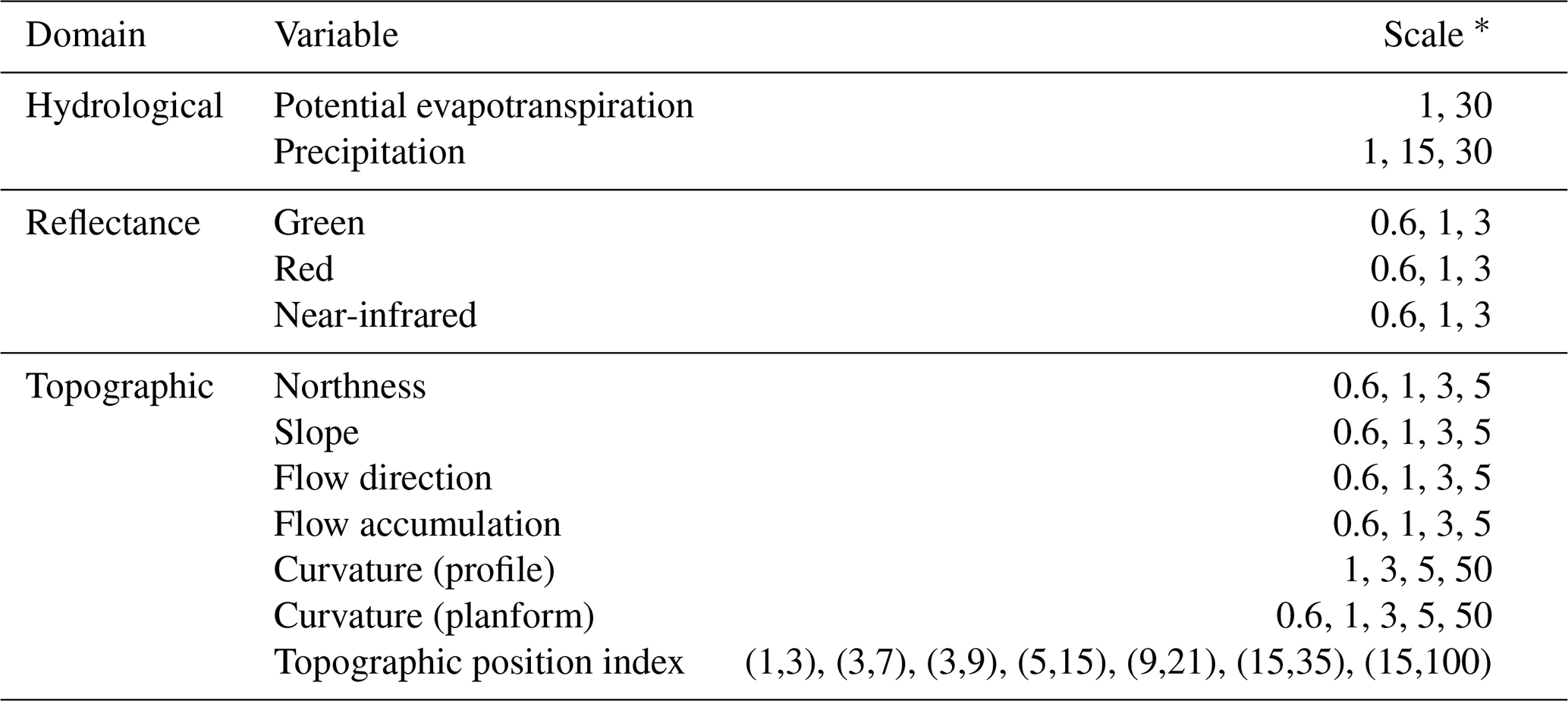
* Scale for raster products is pixel resolution in meters and cumulative days for the hydrological variables. Topographic position index scale is a combination of the inner and outer diameters in meters (see Eq. 1).
Following the variable selection procedure, of the 138 variables, 76 variables were removed based on linear correlation and linear dependencies among variables. An additional 16 were removed following the recursive feature elimination procedure. The final data used for building the models had 46 variables (Table 2), of which five are hydrological, nine are reflectance, and 32 are topographic variables. Variable categories that had no importance included the topographic wetness index (TWI), the reflectance in the red-edge band, and normalized difference vegetation index (NDVI).
2.4 Data description
The 6 data collection days in the 2018 water year and summary site statistics are given in Table 3. Cumulative and 30 d rolling sums of precipitation and PET for the 2018 water year are shown in Figs. S3 and S4.

Figure 5Measured soil moisture and vegetation index of the ground sampling locations from 1 m resolution raster.
Figure 5 shows the distribution of soil moisture and Thiam's transformed vegetation index (TTVI) during the 6 measurement days. The soil moisture measurement followed the general precipitation patterns but was also influenced by immediate rainfall events; the highest soil moisture occurred on the only measurement day on which it had rained the day before (23 January 2018). The vegetation greenness, as measured with TTVI, followed the 15 d cumulative rainfall well, with maximum greenness occurring on 4 April 2018 (day of water year 186) and sharply decreasing in the following 2 months (Fig. 5).
Figure S5 shows the distribution of some terrain variables associated with the soil moisture sampling points and correlations between variables. The terrain variables for the ground sampling points show a reasonable distribution of values, while the distribution of elevation shows a bimodal distribution with ranges from 120 to 130 m; most of the other variables show a close to normal distribution. The only variables with Person's correlation above 0.5 are between TPI and curvature (Pearson's correlation is equal to 0.67). The distribution of some variables in the data is shown in Fig. S6.
2.5 Machine learning procedure
The overall machine learning procedure is illustrated in Fig. 1. The computationally demanding steps of model training and testing were run at the Multi-Environment Research Computer for Exploration and Discovery (MERCED) high-performance computing cluster at the University of California, Merced. The caret R package (v6.0-78; Kuhn, 2008) was used to handle training and tuning procedures. The SVR and relevance vector regression (RVR) algorithms were implemented using the kernlab package (v0.9-26; Karatzoglou et al., 2004), RF algorithm was implemented using the randomForest package (v4.6-12; Liaw and Wiener, 2002), and the BRT algorithm was implemented using the xgboost package (v0.6.4.1; Chen and Guestrin, 2016).
Prior to model training, all the predictor variables were standardized by centering to mean zero and scaling by the variable's standard deviation (Eq. 2) as follows:
where x′ is the centered and scaled value of variable x, and and σx are the arithmetic mean and standard deviation of the variable. Standardizing variables prior to model training is a good practice that minimizes issues of scale among input variables and often leads to better and faster training (Brownlee, 2020).
2.5.1 Machine learning algorithms used
Several machine learning algorithms exist for multivariate regression modeling. Artificial neural networks (ANNs) are among the most commonly used algorithms for the retrieval of soil moisture from remote sensing (e.g., Hassan-Esfahani et al., 2015; Paloscia et al., 2008). In recent years, the support vector machine (SVM) and the similar support vector regression (SVR) algorithms have become popular in the retrieval of soil moisture (e.g., Ahmad et al., 2010; Zaman and Mckee, 2014; Zaman et al., 2012). Other popular machine learning algorithms include tree-based models such as the random forest (RF) and boosted regression trees (BRTs).
Artificial neural network (ANN)
ANN models have been widely used in the development of pedotransfer models (Matei et al., 2017; Pachepsky et al., 1996; Schaap et al., 2001; Zhang et al., 2018; Zhang and Schaap, 2017). ANNs are universal approximators that can approximate any nonlinear mapping. The feed-forward neural network is a popular variant of ANN. In this study, we implemented the feed-forward neural network with a single hidden layer, which is considered sufficient for the majority of problems (Reed and Marks II, 1999).
Support vector regression (SVR)
SVR is an adaptation of the support vector machine (SVM) for regression problems (Cortes and Vapnik, 1995; Drucker et al., 1997). The SVM learning is a generalization of a maximal margin classifier. The algorithm first maps the input variables into a high-dimensional space using a fixed mapping function, i.e., a kernel function. The algorithm then constructs hyperplanes, which can be used for classification or, in the case of SVR, for regression. In this study, we use the radial basis function kernel, which is one of the most-used kernels in SVR. Some advantages of SVR include the fact that they do not suffer from the problem of local minima, and that they have few parameters to tune when training the model.
Relevance vector regression (RVR)
Like SVM, the RVR was originally introduced as a classification machine (Tipping, 2000). RVR is a Bayesian treatment of the SVM prediction function which avoids some of the limitations of SVM algorithms, such as reducing the use of basis functions and the need for optimizing the cost and the insensitivity parameters (Ben-Shimon and Shmilovici, 2006). Torres-Rua et al. (2016) successfully used the RVR algorithm to estimate surface soil moisture from satellite images and energy balance products.
Random forest (RF)
RFs are popular models that are relatively simple to train and tune (Hastie et al., 2009). They apply ensemble techniques by averaging a large number of individual decision-tree-based models. Tree models are grown by searching for a predictor that ensures the best split that results in the smallest model error. The individual trees in the RF ensemble are built on a bootstrapped training sample, and only a small group of predictor variables are considered at each split; this ensures that trees are decorrelated with each other (Breiman, 2001; James et al., 2013).
Boosted regression trees (BRTs)
BRT is another form of the decision tree model ensemble enhanced by the gradient boosting approach. The gradient boosting algorithm constructs additive regression models by sequentially fitting simple base learner functions (i.e., decision trees) to current pseudo-residuals at each iteration (Friedman, 2002). These pseudo-residuals are the gradient of the loss function being minimized. BRT models have shown considerable success and often outperform other machine learning algorithms in many situations (Elith et al., 2008; Natekin and Knoll, 2013). BRT models are also particularly suitable for less-than-clean data (Friedman, 2001), which makes them particularly attractive in our work where the training data are compiled from various sources and different measurement methods, making them prone to some inconsistencies.
Tree-based models, both the RF and BRT, have the advantage of being able to rank the predictor variable's relative importance. In these models, the approximate relative influence of a single predictor variable is calculated as the empirical improvement of predictions by splitting on that predictor at each node and then averaging the relative influence of the variable across all trees of the model (Ridgeway, 2012).
2.5.2 Training–testing set splits
The data was split into training and testing sets of approximately 75 %–25 %, respectively (i.e., approximately 300 and 100 records). The testing set was a hold-out set used only to evaluate final trained models.
The training–testing set splitting was done based on a random selection of the transect. For the testing set, two transects are randomly selected on four randomly selected sampling dates, and one transect is randomly selected on the remaining two sampling dates. To minimize the bias that may result from the training–testing set split, we generated 30 unique training–testing set splits and trained 30 separate models based on each separate training set. The performance of each model was assessed on its respective testing set. Similar performance of the individual models would indicate that bias due to the training–testing set split is minimal. The justification for this subsetting procedure is as follows: (1) the selection of entire transects as testing sets avoids possible data leakage between the training and testing sets due to spatial autocorrelation since samples in a transect are located close to each other – a simple random splitting would not avoid this potential problem; (2) all six sampling dates are represented in the training set – models are trained on the entire range of time and soil moisture changes; and (3) the testing set is between 25 % and 30 % of the data (between 100 and 125 samples).
The distribution of samples across the sampling dates and transects for the training and testing sets is shown in Figs. S7 and S8, respectively. On average, the training–testing split was 294 samples in the training sets and 113 samples in the testing sets. All the training sets have samples from all the six sampling dates and transects. While all sampling dates are represented in each testing set, on average, there are five transects in each testing set.
2.5.3 Cross-validation procedure
The selection of optimal model parameters in the model training process was done by the cross-validation method. Cross validation is done to estimate the test error rate by holding out a subset of the training data (i.e., a validation set) from the fitting process and then applying the fitted model to predict the validation subset. A 30-fold cross-validation set was generated by randomly splitting the training data into 80 %–20 % training–validation split by randomly selecting a single transect every day. Optimum model parameters were selected using a comprehensive grid search method.
2.5.4 Model assessment
Performance
The final performance of models was assessed on the separate hold-out test data set that was not used in the model training. The performance of models is measured in terms of mean absolute error (MAE), mean bias error (MBE), and the coefficient of determination (R2) determined as follows:
where N is the number of observations, y is the measured value, is the predicted value, and is the mean of measured values.
The MAE indicates the average deviation of predictions from the measured value, with smaller values indicating better performance. The MBE measures the average systematic bias, and positive or negative values indicate the average tendency of the predicted values to be larger or smaller than the measured values, respectively. The R2 measures the correspondence between predicted and measured data, with higher values indicating stronger correspondence. The MAE was chosen over RMSE as it is a more appropriate measure when averaging (Willmott and Matsuura, 2005).
Variable importance
The predictor variable importance is the statistical significance of each predictor variable with respect to its effect on the generated model. For the tree-based models, RF and BRT, variable importance is calculated internally within the model algorithm. For the rest of the machine learning models, we calculated the predictor variable importance by the recursive feature elimination method, which is done by recursively removing predictors before training a model and evaluating the change in model performance. In this method, to account for possible bias in variable subset selection (Ambroise and McLachlan, 2002; Hastie et al., 2009), we included a separate layer of 10-fold cross validation in the entire sequence modeling steps.
Effect of predictor variables
The relationship between the predictor variables and outputs for a black box model can be analyzed using model-independent methods such as partial dependence plots or accumulated local effects (ALEs) plots (Apley and Zhu, 2020; Greenwell, 2017). These plots help to explain the relationship between the outcome of the black-box-supervised machine learning models and the predictors of interest. We use the ALE plots to analyze the effect of selected predictor variables. Although similar, the ALE plots are preferred over partial dependence plots for their speed and their ability to produce unbiased plots when variables are correlated (Apley and Zhu, 2020). The value of the ALE is centered so that the mean effect is zero; it can be interpreted as being the effect of the variable on the outcome at a certain value compared to the average prediction of the data. For example, if an ALE estimate of −2 occurs when a variable of interest has a value of 3, then the prediction is lower by 2 compared to the average prediction (Molnar, 2019).
3.1 Model performance
All the tested machine learning algorithms were able to predict soil moisture with good accuracy. Both BRT and RF algorithms, however, had a slightly better performance with a MAE of less than 4 % soil moisture content. Figure 6 shows the performances of the five machine learning algorithms in the testing set. The relatively better performance of BRT and RF models is consistent with other studies that find that ensemble decision-tree-based regression models perform better than many other machine learning algorithms (Caruana and Niculescu-Mizil, 2006), particularly in terrain and soil spatial predictions (Hengl et al., 2017, 2018; Keskin et al., 2019; Nussbaum et al., 2018; Szabó et al., 2019). Of the two best algorithms, BRT performs marginally better, and we present variable importance and predictor effect analysis done with the BRT model. Despite being marginally inferior to BRT, the RF model has several advantages over BRT and the other algorithms. RF is much easier and faster to train compared to the other machine learning algorithms used. Since the ensemble trees are independent in the RF model, the forest can be grown simultaneously, which dramatically increases the processing efficiency in parallel computing. In addition, the RF model has few hyperparameters to tune. In contrast, the ensemble trees in the BRT algorithm must be grown sequentially since each new tree is dependent on the previous ensemble (which makes parallel processing challenging). Training a BRT model requires tuning multiple hyperparameters – seven in our implementation of the BRT model compared to two for the RF model. The performance of individual models across the 30 different training–testing splits was comparable and seems consistent with minimum bias resulting from testing set selection. The performances of the individual 30 tuned BRT models on their respective testing sets are shown in Fig. S9.
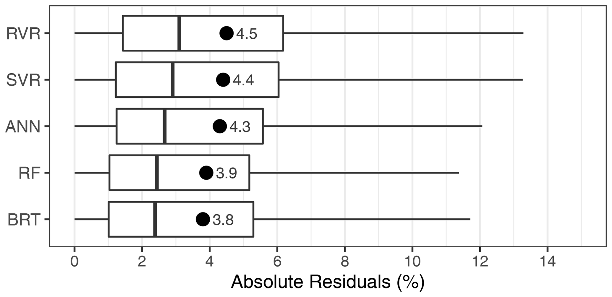
Figure 6Distribution of residuals and MAE on the testing set by the type of machine learning algorithm. Filled circles and values to the right indicate the average MAE.
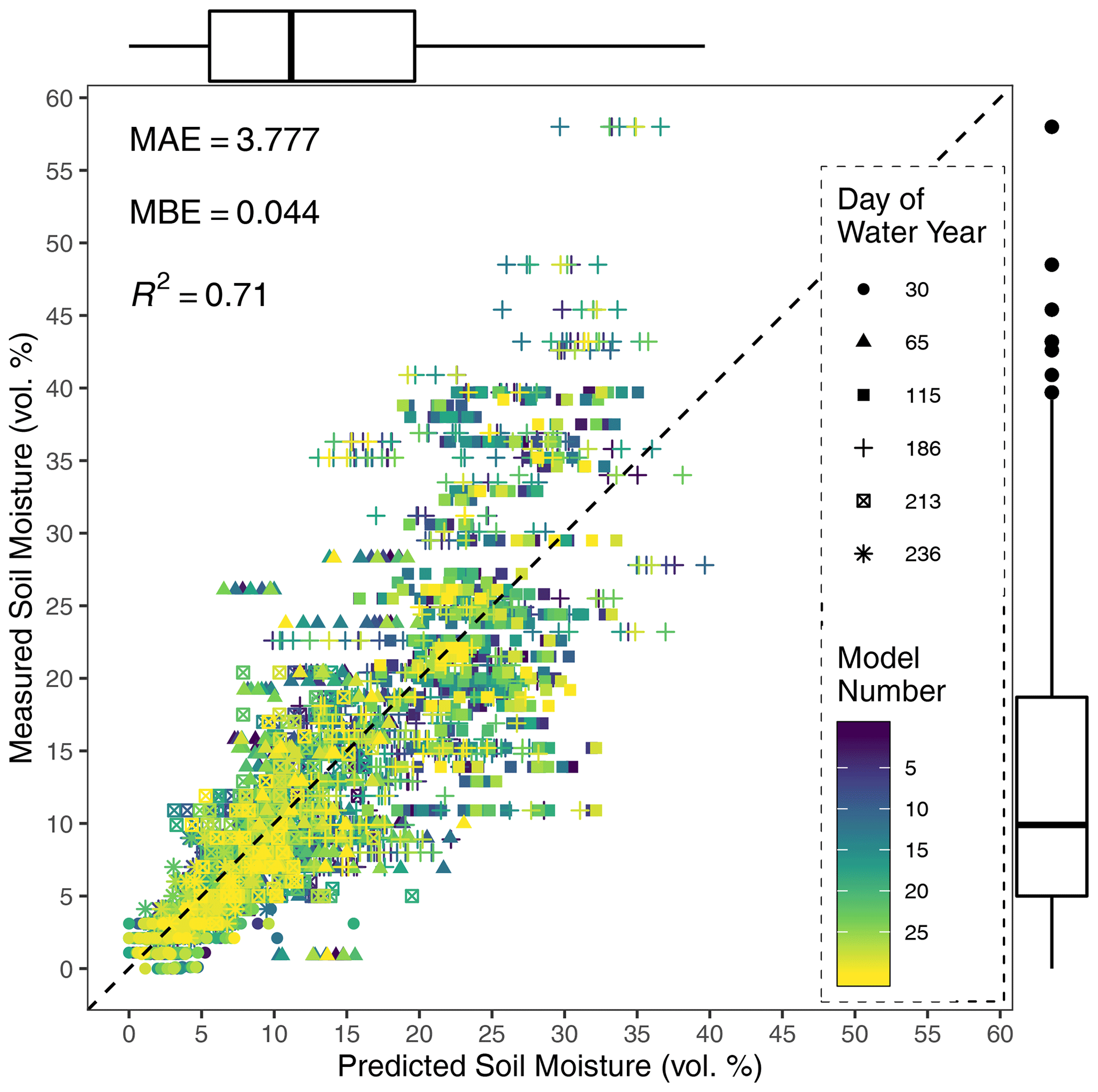
Figure 7Scatterplot of the measured vs. predicted soil moisture content for the testing sets. Marginal box plots show the distributions of measured and predicted values. MAE, MBE, and R2 are averaged across the 30 models.
Measured vs. model-predicted soil moisture contents for the testing data sets are plotted in Fig. 7. The one-to-one comparison in Fig. 7 shows the individual predictions by all 30 models. The plot shows a general increase in error at higher soil moisture levels. In addition, the model prediction appears capped at around 40 % soil moisture content; this is likely the result of a lack of training data points with values above that soil moisture (see Fig. 5). The marginal box plot on the y axis of Fig. 7 illustrates this point as values above a 40 % soil moisture content are over 1.5 times the interquartile range above the upper quartile and are plotted as outliers.
3.2 Predictor variable importance
Precipitation and PET were among the top variables in terms of predictive importance. This is to be expected, given that these two variables represent the major source and loss pathway for surface soil moisture. Reflectance in the red band was by far the most important of all the reflectance bands. Following these three variables, topographic variables – TPI and curvature in particular – were most important in most models. Topography has a strong control on soil moisture distribution at landscape scales (Sørensen et al., 2006), while the TPI was the most important topographic variable in determining soil moisture. A surprising finding was that TWI was found not to be an important predictor despite numerous studies finding it important in explaining surface soil moisture (e.g. Moore et al., 1988; Western et al., 1999) Despite calculating TWI in multiple ways and at multiple scales, it consistently failed the variable selection procedure for all algorithms we tested. The reasons for this could be that TWI is of little significance when explaining soil moisture distribution at a small scale. Upon observing a similar lack of correlation between TWI and soil moisture, Famigliettiet et al. (1998) suggest that TWI is more appropriate for predicting the soil moisture of an entire unsaturated zone profile and not just the surface layer. Yet another reason could be that since slope and flow accumulation, i.e., the constituent parts of TWI, are already included in the models, it was deemed redundant (not providing unique information) to the models. This would be consistent with the models not finding NDVI important when the constituent bands (red and NIR bands) were found to be important.
When considering the importance of variables, it is worth noting that different variables may have different degrees of importance depend on how wet or dry the soil condition is. Western et al. (1999), for example, found that flow accumulation was the best predictor for soil moisture distribution during wet conditions, while the potential solar radiation index was a better predictor during dry conditions.
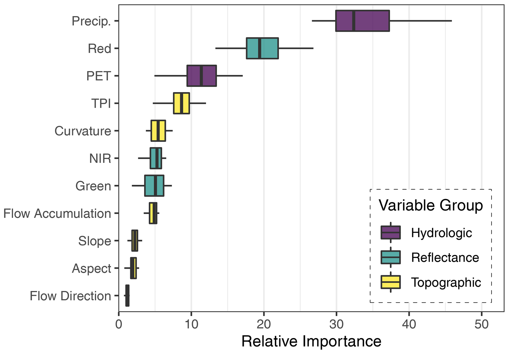
Figure 8Relative variable importance distribution of the 30 BRT models aggregated by variable type.
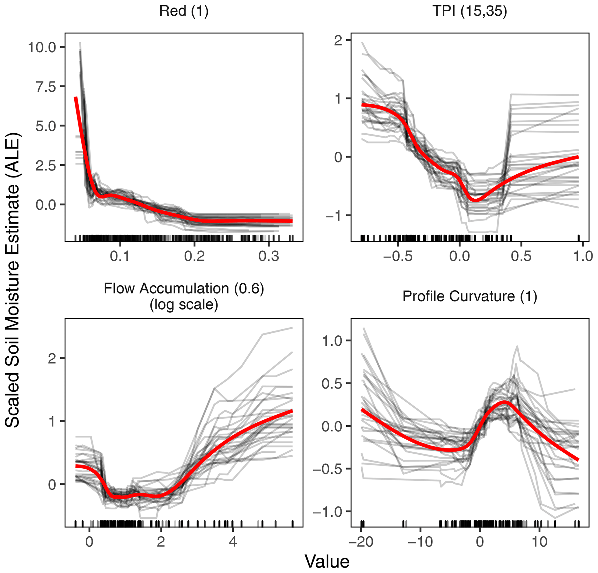
Figure 9ALE plots for four selected high-importance predictor variables. The black curves represent the individual effects of the 30 models, and red curves are smoothed trend lines over all individual models. Marks along the x axis show the distribution of the data in the model training set.
The relative importance of predictors for the BRT model is shown in Fig. 8. The predictors have been grouped by variable type (lumping the same variables regardless of variable specifications, such as summation window for precipitation or pixel resolution for the raster). The only temporally dynamic variables in our model are the hydrological and reflectance variables; the topographic variables are not time dependent, and their variables need only be generated once for a study area. A more detailed variable importance plot is provided in Fig. S10.
3.3 Effect of predictor variables
We used the ALE plots to investigate the nature of the relationship between the predictor variables and soil moisture. Figure 9 shows the partial effect of red reflectance and three of the most important topographic variables, i.e., TPI, profile curvature, and flow accumulation. Given the high importance of these topographic variables, it is useful to understand how these variables relate to soil moisture and identify possible thresholds of significant changes. Predicted soil moisture generally increased with flow accumulation across all scales.
The relationship of curvature to soil moisture is a little more complex; soil moisture tends to decrease as surfaces became less convex. However, the trend reverses, and soil moisture increases as surface curvature transitions from convex to concave (approximately between profile curvature values −5 and +5) before the effect reverses again at higher concavity surfaces. A possible explanation for this behavior might be that more flat surfaces (with a near-zero curvature value) are associated with higher slope areas, such as those immediately following a ridgetop which is of higher convexity. The decreasing trend of soil moisture at increasing concavity (profile curvature value above +5) is harder to explain. However, at lower scales (3 and 5 m resolution DEM), soil moisture did peak at the convex to concave transition (near zero) but there was almost no noticeable decreasing pattern at higher curvature (concavity) values (not presented in this paper). At the lowest resolution (50 m DEM), soil moisture continuously increases with an increase in concavity of surface.
Of all the topographic variables we calculated, perhaps TPI is the most scale-dependent variable. Surprisingly, TPI across all scales had a similar relation with soil moisture. Negative TPI values indicate a surface that trends towards valleys, and zero values indicate flat areas, if the slope of the surface is shallow, or mid-slope areas. For areas with significant slopes, positive TPI values indicate surfaces that trend towards ridgetops (Jenness et al., 2013). Across all scales, there was a U-shaped relation between TPI and soil moisture, with soil moisture decreasing as negative TPI values moved towards zero and soil moisture increasing as TPI moved from zero to positive values. This pattern is consistent with valleys and ridgetops being wetter than mid-slope areas. We computed TPI at several scales, and across all machine learning algorithms, TPI with 15 and 35 m inner and outer diameters, i.e., TPI(15,35), had the highest variable importance among all topographic variables.
Although the machine learning models are considered non-spatial models, as they do not consider sampling location information and spatial autocorrelations (Georganos et al., 2019; Hengl et al., 2018), the inclusion of spatially dependent variables (specifically curvature, flow accumulation, and TPI) as predictors means that the models do account for a significant amount of spatial information. The inclusion of such variables should make the predictions more spatially relevant.
The red band was the most predictive of the three bands, and the red-edge band was found not to be an important predictor. The two spectral vegetation indices we tested, i.e., NDVI and TTVI, were found not to be important, but their constituent bands, the red and NIR, were important. The lower importance of NIR compared to the red band in the prediction of surface soil moisture was particularly surprising, given the higher sensitivity of the NIR band to plant moisture stress and the fact that our study area was almost entirely covered with vegetation.

Figure 10Predicted soil moisture content (percent) over the study area for the 6 d sampled. Days of the water year 30, 65, 115, 186, 213, and 236 are 30 October 2017, 4 December 2017, 23 January 2018, 4 April 2018, 1 May 2018, and 24 May 2018, respectively).
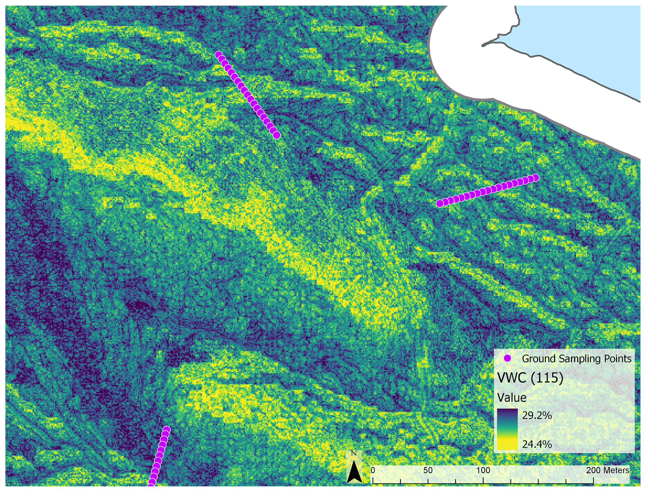
Figure 11Magnified map of predicted soil moisture content (percent) map for water year day 115 (23 January 2018).
3.4 Spatial prediction of soil moisture
The final utility of training a machine learning model was to be able to produce a spatially resolved soil moisture map. In Fig. 10, we have predicted surface soil moisture for the 6 sampling days for which we had multispectral images. Ideally, in the future, the only new inputs required to produce a soil moisture prediction map for our study site is UAV-based multispectral images and hydrologic variables of precipitation and PET which are available from nearby weather stations. As can be seen in Fig. 10, while the mean moisture content was largely driven by the day (which, in turn, is controlled by antecedent precipitation and PET), the distribution appears to closely follow topographic attributes. This is particularly visible in a magnified map (Fig. 11). Ridges appear drier, while valleys appear wetter; furthermore, northern-facing ridges appear slightly drier than south-facing slopes, which is probably due to slightly higher vegetation cover. Density plots showing the distribution of soil moisture predictions over the test area for each of the 6 d is provided in Fig. S11.
A magnified map of the soil moisture prediction for 23 January 2018 is shown in Fig. 11 and shows that soil moisture varies considerably with topography. Tracks made by the repeated passage of vehicles are, for example, clearly identifiable as areas of low soil moisture in the magnified map.
Our study addressed the following questions: how effectively can machine learning methods be employed to retrieve soil moisture from a combination of topographic and UAV remote sensing data? What are the most important predictors of surface soil moisture in our study area? And what is the nature of the relationship between predictor variables and soil moisture? Our approach can be summarized as follows: we took multispectral images of grassland in the visible near-infrared range using a UAS. Using a photogrammetric analysis of the images, we produced a high-resolution digital elevation model of the study site, which we used to calculate several topographic variables at different scales. Simultaneously with the UAS imaging flights, we took about 400 in situ surface soil moisture measurements. Using those ground truth measurements, we trained machine learning models to predict soil moisture from the multispectral images, topographic variables, and precipitation and evapotranspiration data. We finally interrogated the machine learning models to understand the importance of the different variables and elucidate the nature of the relationship between variables and soil moisture.
What makes our study stand out is that we used UAS-based remote sensing to investigate soil water outside of the relatively homogenous farm plots. Our study site had uneven topography and an ecology dominated by large seasonal shifts in moisture. The fact that it is neither bare nor a monoculture makes the interpretation of multispectral images challenging and necessitates the use of machine learning methods that are able to generalize complex relationships. This research serves as a proof of concept that surface soil moisture can be interpreted with reasonable accuracy from multispectral UAS remote sensing using machine learning methods.
Based on our findings, we conclude that all the popular machine learning algorithms we tested (ANN, SVR, RVR, RF, and BRT) are acceptable for modeling surface soil moisture with the conditions of our study. We particularly found that decision-tree-based methods, especially RF, make for a versatile algorithm. Even though its prediction accuracy is only marginally better than the other machine learning algorithms we tested, RF has the advantage of being particularly simple to train and requiring the least amount of computational resources.
Analysis of the models revealed that hydrologic variables of precipitation and evapotranspiration are the most important predictor variables for surface soil moisture. However, spatial distribution of soil moisture is highly dependent on topographic variables. Topographic variables, such as flow accumulation and TPI, are particularly important in ameliorating the non-spatial nature of such machine learning models by including spatial variables. Based on our study, a DEM of about 1 m horizontal resolution is sufficient. Although we had resolution as high as 15 cm, we found that excluding such high-resolution topographic variables did not substantially reduce the model performances.
A partial dependence analysis of how the input variables relate to soil moisture is important for an understanding of the mechanisms that control soil moisture over the landscape. Using a type of partial dependency plot, we were able to investigate the nature of the relationships. Surface curvature showed a complex relationship with soil moisture. Curvature showed a negative relationship with soil moisture as convex surfaces became less convex. This relationship reverses as the convex surfaces transition to concave, with increases in concavity being positively related with soil moisture. This relation reverses again at higher concavities, indicating that the partial effect of the curvature variable is such that the mildly concave surfaces tend to be wetter than more concave surfaces. However, the magnitude of soil moisture changes associated with curvature are small. TPI was the most important of the topographic variables. The partial dependency plots in the form of ALE (Fig. 9) show that it affects soil moisture at a relatively higher magnitude. The general nature of the TPI–soil moisture relation indicates that valleys and ridgetops tend to be wetter surfaces compared to the areas in between. Furthermore, valleys tend to be wetter than ridgetops.
As a data mining technique, machine learning model performance and reliability are closely tied to the quantity of data. Although the number and spatial coverage of ground sampling points were reasonable for the purposes of our research, future studies would benefit from significantly increasing the number of ground measurements and flight frequency. Multi-year studies are eventually needed to ensure that the model can be used reliably for future predictions. As data-based methods, machine learning methods are highly unreliable if used to forecast situations that they have not been trained on.
Another important consideration for future studies is to move beyond surface soil moisture to deeper layers. Although more challenging to implement, studies of root zone soil moisture are generally more ecologically relevant. Expanding the reflectance information beyond multispectral bands could lead to important improvements in soil moisture prediction. Although lightweight thermal or hyperspectral sensors are currently very expensive and may not be financially feasible for routine applications, the market trend is optimistic that those technologies will become more affordable in the future. Another interesting avenue worth investigating is the possibility of using the high-resolution topographic variables from UAS along with cheaper and more widely available satellite images.
Although the machine learning models used in this study have many advantages, one drawback is that they are non-spatial models and, as such, do not consider sampling location information and spatial autocorrelations. This potentially weakens these models' ability to appropriately address spatial heterogeneities (Georganos et al., 2019; Hengl et al., 2018). Hengl et al. (2018) introduce a novel method for incorporating spatial information into a non-spatial machine learning model by including distances between sampling points as predictor variables, and they show that this method (although still in its formative stage) has comparable accuracy to kriging methods. The potential to improve soil moisture predictions by using such spatially integrated methods should be considered in future research.
| ALEs | Accumulated local effects |
| ANN | Artificial neural network |
| BRTs | Boosted regression trees |
| DEM | Digital elevation model |
| MAE | Mean absolute error |
| MBE | Mean bias error |
| NDVI | Normalized difference vegetation index |
| NIR | Near-infrared |
| PET | Potential evapotranspiration |
| RF | Random forest |
| RMSE | Root mean square error |
| RVR | Relevance vector regression |
| SVR | Support vector regression |
| TDR | Time domain reflectometry |
| TPI | Topographic position index |
| TTVI | Thiam's transformed vegetation index |
| UAS | Unoccupied aircraft systems |
The underlying code used in this article is available online at https://doi.org/10.5281/zenodo.4743238 (Araya, 2021).
The underlying data used in this article are available online at https://doi.org/10.5281/zenodo.4743238 (Araya, 2021).
The supplement related to this article is available online at: https://doi.org/10.5194/hess-25-2739-2021-supplement.
SA, TA, and JV contributed to the study design. The ground measurement site survey and setup was done by SA and AF. The ground measurement was conducted by SA. UAS remote sensing and image preprocessing were done by AA and SA. Image analysis and model building were done by SA, with supervision from TA and JV. SA prepared the paper with contributions from all coauthors.
The authors declare that they have no conflict of interest.
We would like to thank Monique Kolster and the University of California, Merced Vernal Pools, and Grassland Reserve of the Natural Reserve Systems. We also thank Francesca Cannizzo of the University of California, Merced, Physical and Environmental Planning team. We gratefully acknowledge the computing time on the Multi-Environment Computer for Exploration and Discovery (MERCED) cluster at the University of California, Merced, which was funded by National Science Foundation (grant no. ACI-1429783).
This research has been supported by the US Fish and Wildlife Service Agreement (grant no. P1740401).
This paper was edited by Giuliano Di Baldassarre and reviewed by Salvatore Manfreda and one anonymous referee.
Ahmad, S., Kalra, A., and Stephen, H.: Estimating soil moisture using remote sensing data: A machine learning approach, Adv. Water Resour., 33, 69–80, https://doi.org/10.1016/j.advwatres.2009.10.008, 2010.
Ali, I., Greifeneder, F., Stamenkovic, J., Neumann, M., and Notarnicola, C.: Review of Machine Learning Approaches for Biomass and Soil Moisture Retrievals from Remote Sensing Data, Remote Sens.-Basel, 7, 16398–16421, https://doi.org/10.3390/rs71215841, 2015.
Ambroise, C. and McLachlan, G. J.: Selection bias in gene extraction on the basis of microarray gene-expression data, P. Natl. Acad. Sci. USA, 99, 6562–6566, https://doi.org/10.1073/pnas.102102699, 2002.
Anderson, K. and Gaston, K. J.: Lightweight unmanned aerial vehicles will revolutionize spatial ecology, Front. Ecol. Environ., 11, 138–146, https://doi.org/10.1890/120150, 2013.
Apley, D. W. and Zhu, J.: Visualizing the effects of predictor variables in black box supervised learning models, Roy. Stat. Soc. B, 82, 1059–1086, https://doi.org/10.1111/rssb.12377, 2020.
Araya, S. N.: saraya209/uas-soil-moisture: First release of uas-soil-moisture code and data, Zenodo, https://doi.org/10.5281/zenodo.4743238, 2021.
Barrett, B. W. and Petropoulos, G. P.: Satellite Remote Sensing of Surface Soil Moisture, in: Remote Sensing of Energy Fluxes and Soil Moisture Content, edited by: Petropoulos, G. P., CRC Press, Boca Raton, FL, 85–120, 2014.
Ben-Dor, E., Chabrillat, S., Demattê, J. A. M., Taylor, G. R., Hill, J., Whiting, M. L., and Sommer, S.: Using Imaging Spectroscopy to study soil properties, Remote Sens. Environ., 113 (Suppl. 1), S38–S55, https://doi.org/10.1016/j.rse.2008.09.019, 2009.
Ben-Shimon, D. and Shmilovici, A.: Kernels for the Relevance Vector Machine – An Empirical Study, in: Advances in Web Intelligence and Data Mining, edited by: Last, M., Szczepaniak, P. S., Volkovich, Z., and Kandel, A., Springer-Verlag GmbH, Berlin, Heidelberg, 253–263, 2006.
Berni, J. A. J., Zarco-Tejada, P. J., Suárez, L., González-Dugo, V., and Fereres, E.: Remote sensing of vegetation from UAV platforms using lightweight multispectral and thermal imaging sensors, Int. Arch. Photogramm., 38, 6, https://doi.org/10.1007/s11032-006-9022-5, 2009.
Breiman, L.: Random Forest, Mach. Learn., 45, 5–32, https://doi.org/10.1023/A:1010933404324, 2001.
Brownlee, J.: Better Deep Learning Train Faster, Reduce Overfitting, and Make Better Predictions, 1.8., Machine Learning Mastery Pty., available at: https://machinelearningmastery.com/better-deep-learning/ (last access: 7 May 2021), 2020.
California Department of Water Resources: UC Merced Weather Station, available at: http://cdec.water.ca.gov/dynamicapp/staMeta?station_id=UCM (last access: 1 February 2019), 2018.
California Irrigation Management Information System: CIMIS Station Report, available at: https://cimis.water.ca.gov/WSNReportCriteria.aspx (last access: 1 February 2019), 2018.
California Irrigation Management Information System: Data Overview, available at: https://cimis.water.ca.gov/Resources.aspx, last access: 19 April 2019.
Caruana, R. and Niculescu-Mizil, A.: An empirical comparison of supervised learning algorithms, in: Proceedings of the 23rd international conference on Machine learning – ICML '06, ACM Press, New York, USA, 161–168, 2006.
Chen, T. and Guestrin, C.: XGBoost: A Scalable Tree Boosting System, in: Proceedings of the 22nd ACM SIGKDD International Conference on Knowledge Discovery and Data Mining - KDD '16, ACM Press, New York, USA, 785–794, 2016.
Chen, X. and Jeong, J. C.: Enhanced Recursive Feature Elimination, in: Proc. – 6th Int. Conf. Mach. Learn. Appl. ICMLA 2007, 13–15 December 2007, Cincinnati, OH, USA, 330–335, https://doi.org/10.1109/ICMLA.2007.35, 2007.
Colomina, I. and Molina, P.: Unmanned aerial systems for photogrammetry and remote sensing: A review, ISPRS J. Photogramm., 92, 79–97, https://doi.org/10.1016/j.isprsjprs.2014.02.013, 2014.
Cortes, C. and Vapnik, V. N.: Support-Vector Networks, Mach. Learn., 20, 273–297, https://doi.org/10.1023/A:1022627411411, 1995.
Das, N. N. and Mohanty, B. P.: Root Zone Soil Moisture Assessment Using Remote Sensing and Vadose Zone Modeling, Vadose Zone J., 5, 296, https://doi.org/10.2136/vzj2005.0033, 2006.
Drucker, H., Burges, C. J. C., Kaufman, L., Smola, A., and Vapnik, V. N.: Support vector regression machines, in: Advances in Neural Information Processing Systems 9: Proceedings of the 1996 Conference, edited by: Mozer, M. C., Jordan, M. I., and Petsche, T., MIT Press, Cambridge, Massachusetts, 155–161, 1997.
Elarab, M.: The Application of Unmanned Aerial Vehicle to Precision Agriculture: Chlorophyll, Nitrogen, and Evapotranspiration Estimation, Utah State University, Utah, 2016.
Elith, J., Leathwick, J. R., and Hastie, T.: A working guide to boosted regression trees, J. Anim. Ecol., 77, 802–813, https://doi.org/10.1111/j.1365-2656.2008.01390.x, 2008.
Famiglietti, J. S., Rudnicki, J. W., and Rodell, M.: Variability in surface moisture content along a hillslope transect: Rattlesnake Hill, Texas, J. Hydrol., 210, 259–281, https://doi.org/10.1016/S0022-1694(98)00187-5, 1998.
Friedman, J. H.: Greedy Function Approximation: A Gradient Boosting Machine, Ann. Stat., 29, 1189–1232, https://doi.org/10.1017/CBO9781107415324.004, 2001.
Friedman, J. H.: Stochastic gradient boosting, Comput. Stat. Data An., 38, 367–378, https://doi.org/10.1016/S0167-9473(01)00065-2, 2002.
Fryjoff-Hung, A. F.: 2D Hydrodynamic Modeling for Evaluating Restoration Potential of a Vernal Pool Complex, University of California, Merced, 2018.
Georganos, S., Grippa, T., Gadiaga, A. N., Linard, C., Lennert, M., Vanhuysse, S., Mboga, N. O., Wolff, E., and Kalogirou, S.: Geographical Random Forests: A Spatial Extension of the Random Forest Algorithm to Address Spatial Heterogeneity in Remote Sensing and Population Modelling, Geocarto Int., 36, 121–136, https://doi.org/10.1080/10106049.2019.1595177, 2019.
Greenwell, B. M.: pdp: An R Package for Constructing Partial Dependence Plots, R J., 9, available at: https://github.com/bgreenwell/pdp/issues (last access: 13 June 2019), 2017.
Guyon, I. and Elisseeff, A.: An Introduction to Variable and Feature Selection, J. Mach. Learn. Res., 3, 1157–1182, 2003.
Guyon, I., Weston, J., Barnhill, S., and Vapnik, V.: Gene selection for cancer classification using support vector machines, Mach. Learn., 46, 389–422, https://doi.org/10.1023/A:1012487302797, 2002.
Hassan-Esfahani, L., Torres-Rua, A., Jensen, A., and McKee, M.: Assessment of surface soil moisture using high-resolution multi-spectral imagery and artificial neural networks, Remote Sens.-Basel, 7, 2627–2646, https://doi.org/10.3390/rs70302627, 2015.
Hastie, T., Tibshirani, R., and Friedman, J.: The Elements of Statistical Learning: Data Mining, Inference, and Prediction, 2nd edn., Springer New York, New York, NY, 2009.
Haubrock, S.-N., Chabrillat, S., Lemmnitz, C., and Kaufmann, H.: Surface soil moisture quantification models from reflectance data under field conditions, Int. J. Remote Sens., 29, 3–29, https://doi.org/10.1080/01431160701294695, 2008.
Hengl, T., Mendes de Jesus, J., Heuvelink, G. B. M., Ruiperez Gonzalez, M., Kilibarda, M., Blagotić, A., Shangguan, W., Wright, M. N., Geng, X., Bauer-Marschallinger, B., Guevara, M. A., Vargas, R., MacMillan, R. A., Batjes, N. H., Leenaars, J. G. B., Ribeiro, E., Wheeler, I., Mantel, S., and Kempen, B.: SoilGrids250m: Global gridded soil information based on machine learning, edited by: Bond-Lamberty, B., PLoS One, 12, e0169748, https://doi.org/10.1371/journal.pone.0169748, 2017.
Hengl, T., Nussbaum, M., Wright, M. N., Heuvelink, G. B. M., and Gräler, B.: Random forest as a generic framework for predictive modeling of spatial and spatio-temporal variables, PeerJl, 6, e5518, https://doi.org/10.7717/peerj.5518, 2018.
Hillel, D.: Environmental Soil Physics, Academic Press, San Diego, CA, 1998.
James, G., Witten, D., Hastie, T., and Tibshirani, R.: An Introduction to Statistical Learning, Springer New York, New York, NY, 2013.
Jenness, J., Brost, B., and Beier, P.: Land Facet Corridor Designer, available at: http://www.corridordesign.org (last access: 13 June 2019), 2013.
Karatzoglou, A., Smola, A., Hornik, K., and Zeileis, A.: kernlab – An S4 Package for Kernel Methods in R, J. Stat. Softw., 11, 1–20, https://doi.org/10.18637/jss.v011.i09, 2004.
Keskin, H., Grunwald, S., and Harris, W. G.: Digital mapping of soil carbon fractions with machine learning, Geoderma, 339, 40–58, https://doi.org/10.1016/j.geoderma.2018.12.037, 2019.
Korres, W., Reichenau, T. G., Fiener, P., Koyama, C. N., Bogena, H. R., Cornelissen, T., Baatz, R., Herbst, M., Diekkrüger, B., Vereecken, H., and Schneider, K.: Spatio-temporal soil moisture patterns – A meta-analysis using plot to catchment scale data, J. Hydrol., 520, 326–341, https://doi.org/10.1016/j.jhydrol.2014.11.042, 2015.
Kuhn, M.: Building Predictive Models in R Using the caret Package, J. Stat. Softw., 28, 1–26, https://doi.org/10.18637/jss.v028.i05, 2008.
Liaw, A. and Wiener, M.: Classification and Regression by randomForest, R News, 2, 18–22, 2002.
Malley, D. F., Martin, P. D., and Ben-Dor, E.: Application in Analysis of Soils, in: Near-Infrared Spectroscopy in Agriculture, edited by: Craig, R., Windham, R., and Workman, J., American Society of Agronomy, Crop Science Society of America, Soil Science Society of America, Madison, WI, USA, 729–784, 2004.
Manfreda, S., McCabe, M., Miller, P., Lucas, R., Pajuelo Madrigal, V., Mallinis, G., Ben Dor, E., Helman, D., Estes, L., Ciraolo, G., Müllerová, J., Tauro, F., de Lima, M., de Lima, J., Maltese, A., Frances, F., Caylor, K., Kohv, M., Perks, M., Ruiz-Pérez, G., Su, Z., Vico, G., and Toth, B.: On the Use of Unmanned Aerial Systems for Environmental Monitoring, Remote Sens.-Basel, 10, 641, https://doi.org/10.3390/rs10040641, 2018.
Matei, O., Rusu, T., Petrovan, A., and Mihuţ, G.: A Data Mining System for Real Time Soil Moisture Prediction, Procedia Engineer., 181, 837–844, https://doi.org/10.1016/j.proeng.2017.02.475, 2017.
Molnar, C.: Interpretable Machine Learning: A Guide for Making Black Box Models Explainable, Git Hub, available at: https://christophm.github.io/interpretable-ml-book/, last access: 13 June 2019.
Moore, I. D., Burch, G. J., and Mackenzie, D. H.: Topographic Effects on the Distribution of Surface Soil Water and the Location of Ephemeral Gullies, T. ASAE, 31, 1098–1107, https://doi.org/10.13031/2013.30829, 1988.
Muller, E. and Décamps, H.: Modeling soil moisture–reflectance, Remote Sens. Environ., 76, 173–180, https://doi.org/10.1016/S0034-4257(00)00198-X, 2000.
Natekin, A. and Knoll, A.: Gradient boosting machines, a tutorial, Front. Neurorobotics, 7, 1–11, https://doi.org/10.3389/fnbot.2013.00021, 2013.
Nichols, S., Zhang, Y., and Ahmad, A.: Review and evaluation of remote sensing methods for soil-moisture estimation, J. Photon. Energy, 2, 028001, https://doi.org/10.1117/1.3534910, 2011.
Nussbaum, M., Spiess, K., Baltensweiler, A., Grob, U., Keller, A., Greiner, L., Schaepman, M. E., and Papritz, A.: Evaluation of digital soil mapping approaches with large sets of environmental covariates, SOIL, 4, 1–22, https://doi.org/10.5194/soil-4-1-2018, 2018.
Ochsner, T. E., Cosh, M. H., Cuenca, R. H., Dorigo, W. A., Draper, C. S., Hagimoto, Y., Kerr, Y. H., Njoku, E. G., Small, E. E., and Zreda, M.: State of the Art in Large-Scale Soil Moisture Monitoring, Soil Sci. Soc. Am. J., 77, 1888, https://doi.org/10.2136/sssaj2013.03.0093, 2013.
Pachepsky, Y. A., Timlin, D., and Varallyay, G.: Artificial Neural Networks to Estimate Soil Water Retention from Easily Measurable Data, Soil Sci. Soc. Am. J., 60, 727–733, https://doi.org/10.2136/sssaj1996.03615995006000030007x, 1996.
Paloscia, S., Pampaloni, P., Pettinato, S., and Santi, E.: A Comparison of Algorithms for Retrieving Soil Moisture from ENVISAT/ASAR Images, IEEE T. Geosci. Remote, 46, 3274–3284, https://doi.org/10.1109/TGRS.2008.920370, 2008.
Petropoulos, G. P., Ireland, G., and Barrett, B. W.: Surface soil moisture retrievals from remote sensing: Current status, products & future trends, Phys. Chem. Earth, 83–84, 36–56, https://doi.org/10.1016/j.pce.2015.02.009, 2015.
Price, J. C.: Thermal inertia mapping: A new view of the earth, J. Geophys. Res., 82, 2582–2590, 1977.
Price, J. C.: On the analysis of thermal infrared imagery: The limited utility of apparent thermal inertia, Remote Sens. Environ., 18, 59–73, https://doi.org/10.1016/0034-4257(85)90038-0, 1985.
Rana, G. and Katerji, N.: Measurement and estimation of actual evapotranspiration in the field under Mediterranean climate: a review, Eur. J. Agron., 13, 125–153, https://doi.org/10.1016/S1161-0301(00)00070-8, 2000.
Reed, R. and Marks II, R. J.: Neural Smithing: Supervised Learning in Feedforward Artificial Neural Networks, MIT Press, Cambridge, Massachusetts, 1999.
Ridgeway, G.: Generalized Boosted Models: A guide to the gbm package, available at: https://cran.r-project.org/web/packages/gbm/vignettes/gbm.pdf (last access: 1 January 2018) 2012.
Schaap, M. G., Leij, F. J., and van Genuchten, M. T.: Rosetta: A computer program for estimating soil hydraulic parameters with hierarchical pedotransfer functions, J. Hydrol., 251, 163–176, https://doi.org/10.1016/S0022-1694(01)00466-8, 2001.
Schanda, E.: Physical Fundamentals of Remote Sensing, Springer-Verlag, Berlin, Germany, 1986.
Seneviratne, S. I., Corti, T., Davin, E. L., Hirschi, M., Jaeger, E. B., Lehner, I., Orlowsky, B., and Teuling, A. J.: Investigating soil moisture-climate interactions in a changing climate: A review, Earth-Sci. Rev., 99, 125–161, https://doi.org/10.1016/j.earscirev.2010.02.004, 2010.
Singh, K. K. and Frazier, A. E.: A meta-analysis and review of unmanned aircraft system (UAS) imagery for terrestrial applications, Int. J. Remote Sens., 39, 5078–5098, https://doi.org/10.1080/01431161.2017.1420941, 2018.
Sobrino, J., Mattar, C., Jiménez-Muñoz, J. C., Franch, B., and Corbari, C.: On the Synergy between Optical and TIR Observations for the Retrieval of Soil Moisture Content, in: Remote Sensing of Energy Fluxes and Soil Moisture Content, edited by: Petropoulos, G. P., CRC Press, Boca Raton, FL, 363–390, 2014.
Sørensen, R., Zinko, U., and Seibert, J.: On the calculation of the topographic wetness index: evaluation of different methods based on field observations, Hydrol. Earth Syst. Sci., 10, 101–112, https://doi.org/10.5194/hess-10-101-2006, 2006.
Stark, B., McGee, M., and Chen, Y.: Short wave infrared (SWIR) imaging systems using small Unmanned Aerial Systems (sUAS), in: IEEE 2015 International Conference on Unmanned Aircraft Systems (ICUAS), 9–12 June 2015, Denver, CO, 495–501, 2015.
Szabó, B., Szatmári, G., Takács, K., Laborczi, A., Makó, A., Rajkai, K., and Pásztor, L.: Mapping soil hydraulic properties using random-forest-based pedotransfer functions and geostatistics, Hydrol. Earth Syst. Sci., 23, 2615–2635, https://doi.org/10.5194/hess-23-2615-2019, 2019.
Tian, J., Su, H., He, H., and Sun, X.: An Empirical Method of Estimating Soil Thermal Inertia, Adv. Meteorol., 2015, 1–9, https://doi.org/10.1155/2015/428525, 2015.
Tipping, M. E.: The Relevance Vector Machine, in: Advances in Neural Information Processing Systems 12, edited by: Solla, S. A., Leen, T. K., and Muller, K., MIT Press, Cambridge, MA, 652–658, 2000.
Tmušić, G., Manfreda, S., Aasen, H., James, M. R., Gonçalves, G., Ben-Dor, E., Brook, A., Polinova, M., Arranz, J. J., Mészáros, J., Zhuang, R., Johansen, K., Malbeteau, Y., de Lima, I. P., Davids, C., Herban, S., and McCabe, M. F.: Current Practices in UAS-based Environmental Monitoring, Remote Sens.-Basel, 12, 1001, https://doi.org/10.3390/rs12061001, 2020.
Torres-Rua, A., Ticlavilca, A., Bachour, R., and McKee, M.: Estimation of Surface Soil Moisture in Irrigated Lands by Assimilation of Landsat Vegetation Indices, Surface Energy Balance Products, and Relevance Vector Machines, Water, 8, 167, https://doi.org/10.3390/w8040167, 2016.
Trenberth, K. E., Fasullo, J. T., and Kiehl, J.: Earth's Global Energy Budget, B. Am. Meteorol. Soc., 90, 311–323, https://doi.org/10.1175/2008BAMS2634.1, 2009.
Vereecken, H., Huisman, J. A., Pachepsky, Y. A., Montzka, C., van der Kruk, J., Bogena, H., Weihermüller, L., Herbst, M., Martinez, G., and Vanderborght, J.: On the spatio-temporal dynamics of soil moisture at the field scale, J. Hydrol., 516, 76–96, https://doi.org/10.1016/j.jhydrol.2013.11.061, 2014.
Weidong, L., Baret, F., Xingfa, G., Qingxi, T., Lanfen, Z., and Bing, Z.: Relating soil surface moisture to reflectance, Remote Sens. Environ., 81, 238–246, https://doi.org/10.1016/S0034-4257(01)00347-9, 2002.
Western, A. W., Grayson, R. B., Blöschl, G., Willgoose, G. R., and McMahon, T. A.: Observed spatial organization of soil moisture and its relation to terrain indices, Water Resour. Res., 35, 797–810, https://doi.org/10.1029/1998WR900065, 1999.
Weston, J., Elisseeff, A., Schölkopf, B., and Tipping, M.: Use of the Zero-Norm with Linear Models and Kernel Methods, J. Mach. Learn. Res., 3, 1439–1461, 2003.
Whiting, M. L., Li, L., and Ustin, S. L.: Predicting water content using Gaussian model on soil spectra, Remote Sens. Environ., 89, 535–552, https://doi.org/10.1016/j.rse.2003.11.009, 2004.
Willmott, C. and Matsuura, K.: Advantages of the mean absolute error (MAE) over the root mean square error (RMSE) in assessing average model performance, Clim. Res., 30, 79–82, https://doi.org/10.3354/cr030079, 2005.
Wilson, J. P. and Gallant, J. C.: Digital Terrain Analysis, in: Terrain Analysis: principles and applications, edited by: Wilson, J. P. and Gallant, J. C., John Wiley & Sons, Inc, New York, NY, 1–21, 2000.
Wong, K.: Merced Vernal Pools Joins Natural Reserve System, Univ. Calif. News, 22 January 2014, available at: http://universityofcalifornia.edu/news/merced-vernal-pools-join-natural-reserve-system (last access: 5 August 2020), 2014.
Zaman, B. and Mckee, M.: Spatio-Temporal Prediction of Root Zone Soil Moisture Using Multivariate Relevance Vector Machines, Open J. Mod. Hydrol., 4, 80–90, https://doi.org/10.4236/ojmh.2014.43007, 2014.
Zaman, B., McKee, M., and Neale, C. M. U.: Fusion of remotely sensed data for soil moisture estimation using relevance vector and support vector machines, Int. J. Remote Sens., 33, 6516–6552, https://doi.org/10.1080/01431161.2012.690540, 2012.
Zhang, D. and Zhou, G.: Estimation of Soil Moisture from Optical and Thermal Remote Sensing: A Review, Sensors, 16, 1308, https://doi.org/10.3390/s16081308, 2016.
Zhang, Y. and Schaap, M. G.: Weighted recalibration of the Rosetta pedotransfer model with improved estimates of hydraulic parameter distributions and summary statistics (Rosetta3), J. Hydrol., 547, 39–53, https://doi.org/10.1016/j.jhydrol.2017.01.004, 2017.
Zhang, Y., Schaap, M. G., and Zha, Y.: A High-Resolution Global Map of Soil Hydraulic Properties Produced by a Hierarchical Parameterization of a Physically Based Water Retention Model, Water Resour. Res., 54, 9774–9790, https://doi.org/10.1029/2018WR023539, 2018.
Zreda, M., Shuttleworth, W. J., Zeng, X., Zweck, C., Desilets, D., Franz, T., and Rosolem, R.: COSMOS: the COsmic-ray Soil Moisture Observing System, Hydrol. Earth Syst. Sci., 16, 4079–4099, https://doi.org/10.5194/hess-16-4079-2012, 2012.