the Creative Commons Attribution 4.0 License.
the Creative Commons Attribution 4.0 License.
 | 20 May 2021
A Bayesian approach to understanding the key factors influencing temporal variability in stream water quality – a case study in the Great Barrier Reef catchments
Dongryeol Ryu
J. Angus Webb
Anna Lintern
Danlu Guo
David Waters
Andrew W. Western
Stream water quality is highly variable both across space and time. Water quality monitoring programmes have collected a large amount of data that provide a good basis for investigating the key drivers of spatial and temporal variability. Event-based water quality monitoring data in the Great Barrier Reef catchments in northern Australia provide an opportunity to further our understanding of water quality dynamics in subtropical and tropical regions. This study investigated nine water quality constituents, including sediments, nutrients and salinity, with the aim of (1) identifying the influential environmental drivers of temporal variation in flow event concentrations and (2) developing a modelling framework to predict the temporal variation in water quality at multiple sites simultaneously. This study used a hierarchical Bayesian model averaging framework to explore the relationship between event concentration and catchment-scale environmental variables (e.g. runoff, rainfall and groundcover conditions). Key factors affecting the temporal changes in water quality varied among constituent concentrations and between catchments. Catchment rainfall and runoff affected in-stream particulate constituents, while catchment wetness and vegetation cover had more impact on dissolved nutrient concentration and salinity. In addition, in large dry catchments, antecedent catchment soil moisture and vegetation had a large influence on dissolved nutrients, which highlights the important effect of catchment hydrological connectivity on pollutant mobilisation and delivery.
- Article
(10659 KB) - Full-text XML
-
Supplement
(2259 KB) - BibTeX
- EndNote


In-stream water quality plays a vital role in influencing the health of freshwater ecosystems (Pérez-Gutiérrez et al., 2017), which in turn underpins environmental, social and economic sustainability (McGrane, 2016; Ustaoğlu et al., 2020). Pollution derived from agricultural land and urban development has led to water quality degradation in streams and lakes in many regions of the world (Ren et al., 2003). Among these water quality issues, coastal regions with high agricultural production have been delivering large amounts of pollutants to the ocean, where marine ecosystems are vulnerable to the evaluated levels of nutrients and sediments (Gorman et al., 2009). It is estimated that 60 % of coastal rivers in the USA have been moderately to severely degraded (Gorman et al., 2009; Howarth et al., 2002). Therefore, to protect both freshwater and marine ecosystems, better management of catchment-derived pollutants is needed.
Surface water quality is highly variable across spatial and temporal scales (Guo et al., 2019; Lintern et al., 2018a). These spatial and temporal variations are the result of complex interactions between four key pollutant processes in catchments, namely, sources (e.g. atmospheric deposition or anthropogenic inputs), mobilisation (e.g. detachment from the sources), delivery (e.g. transport from sources to receiving waters) and transformation (e.g. biogeochemical processes; Granger et al., 2010; Harris, 2001; Lintern et al., 2018a). Across different catchments, spatial differences in water quality concentration can vary markedly due, in part, to heterogeneity of natural landscapes in catchments (e.g. geology, topography and climate) and human-induced activities (e.g. agricultural and urban development; Liu et al., 2018; Mainali et al., 2019). At a site, water quality concentrations can also exhibit significant daily, event, seasonal and annual variability driven by variations in climatic conditions, in-stream biogeochemical processes and hydrological transport (Thompson et al., 2011). Thus, it can be challenging to design effective catchment water quality management strategies without a sound understanding of the spatial and temporal variation in water quality and the associated driving factors.
While it has been acknowledged that both spatial and temporal variations in water quality are of great importance for effective water resources management (Guo et al., 2020), this study focused on identifying key drivers of the temporal variability in water quality. It follows our previous study investigating spatial variation in water quality in the same region (Liu et al., 2018). A wide range of environmental factors may affect temporal changes in water quality. Runoff and rainfall have been considered as important factors and the most commonly used explanatory variables to describe temporal variation in water quality (Deletic and Maksimovic, 1998), for example, early work by Hem (1948) and Walling (1984). Studies considering hydrometeorological drivers have been typically related to the mobilisation and delivery of pollutants. Catchment soil moisture and evapotranspiration can also have an important role in determining the hydrological cycle (e.g. runoff generation), such as sediments (Bieger et al., 2014), nutrients (Lam et al., 2010) and salinity (Brevik et al., 2006; Tweed et al., 2007), thereby affecting the surface water quality. In addition, riverine water quality has been found to be strongly influenced by seasonal changes in vegetation cover (de Mello et al., 2018; Griffith et al., 2002; Shi et al., 2017). For instance, satellite-derived vegetation indices have provided an opportunity to explore the relationship between land cover and water quality temporal dynamics (Griffith, 2002; Singh et al., 2013). Even though significant research efforts have been made to explore the relationship between water quality and these environmental conditions, a comprehensive understanding of their relative importance in diverse environments and at large scales is still lacking.
Process-based and statistical modelling approaches have been widely used to investigate water quality temporal dynamics in response to changes in the above-mentioned environmental factors (Fu et al., 2019; Wellen et al., 2015). Process-based water quality models use complex mass balance structures describing the water quality source, mobilisation and transport processes (Abbott et al., 1986; Merritt et al., 2003). They are typically based on hydrological and biogeochemical processes that can affect the generation and transport of pollutants into receiving waters. These models (e.g. Soil and Water Assessment Tool – SWAT – and source catchments) have been applied to assess the impact of land use management and climate on sediment and pollutant concentrations (Arnold and Fohrer, 2005; Francesconi et al., 2016; Qi et al., 2018), optimise water management and delivery for agriculture, industry and environmental uses (Ly et al., 2019), and estimate pollutant generation, loss and transport processes (Jayakrishnan et al., 2005; McCloskey et al., 2021). However, the complexity of process-based models results in intensive data and calibration requirements, and large-scale application has been limited (Abbaspour et al., 2015; Arnold and Fohrer, 2005). These models may also have large uncertainties in the interpretability of the parameters and their characterisation of the effects of specific processes (Wade et al., 2002), such as denitrification in streams (Filoso et al., 2004).
On the other hand, statistical water quality models have a relatively simple mathematical structure, an ability to quantify predictive uncertainty (Kasiviswanathan and Sudheer, 2013; Srivastav et al., 2007) and low requirement for a priori information on distinct processes (Letcher et al., 2002; Mainali et al., 2019; Schwarz et al., 2006). However, existing statistical water quality modelling studies have limitations. First, water quality monitoring data have often been limited to low sampling frequencies, typically using monthly grab samples. This can result in a lack of information on water quality dynamics over runoff and/or storm events, which is when a significant proportion of nutrients and sediment loads are transported (Lloyd et al., 2016; Sherriff et al., 2015). Second, most studies on statistical water quality modelling have only investigated the relationship between water quality and explanatory variables in a single or limited number of catchments in small regions (Chang et al., 2015; Khan et al., 2020; Koci et al., 2020). Few studies have investigated water quality at multiple locations using the same modelling framework. Lastly, studies have usually relied on a single best model with an assumption that it best approximated the true drivers of water quality (Paliwal et al., 2007; Zhang et al., 2009). This ignores the issue of selection uncertainty. Furthermore, relying on a single model structure might result in misleading conclusions or overconfidence in the results (Wintle et al., 2003).
This study attempted to address these knowledge gaps in statistical water quality models, taking advantages of event-based water quality monitoring data from the Great Barrier Reef (GBR) catchments in northern Australia, where land-derived pollutants have posed threats to ecosystem health of the GBR lagoon (Brodie et al., 2012; McKergow et al., 2005b). We address the limitations in statistical water quality models by using the following: (1) Bayesian hierarchical modelling was used to investigate water quality temporal variation, which allowed the prediction of water quality in multiple catchments and, simultaneously, quantified parameter uncertainty (Gelman et al., 2013; Rode et al., 2010; Webb and King, 2009); and (2) Bayesian model averaging (BMA) approaches were used to identify the relative importance of the different environmental factors and provide multi-model weighted predictions, which have been shown to better quantify the uncertainty arising from model selection (Höge et al., 2019; Raftery et al., 1997; Wang et al., 2012). We targeted nine common water quality indicators, including sediments, nutrients and salinity. This is a subset of the constituents that have been monitored in the GBR water quality monitoring programme. Our analyses are conducted on constituents that are of great concern to the coral reef ecosystem (McCloskey et al., 2017) and could provide a useful comprehensive picture on the overall water quality status. Finally, we have constrained the variables to only the real parameters that can be directly measured (with the exception of NOx), which helps to understand full sediment and nutrient loads being exported to the GBR lagoon. Overall, this study aimed to (1) identify the key drivers of temporal variation in water quality and (2) predict water quality temporal variation using a Bayesian multi-model approach.
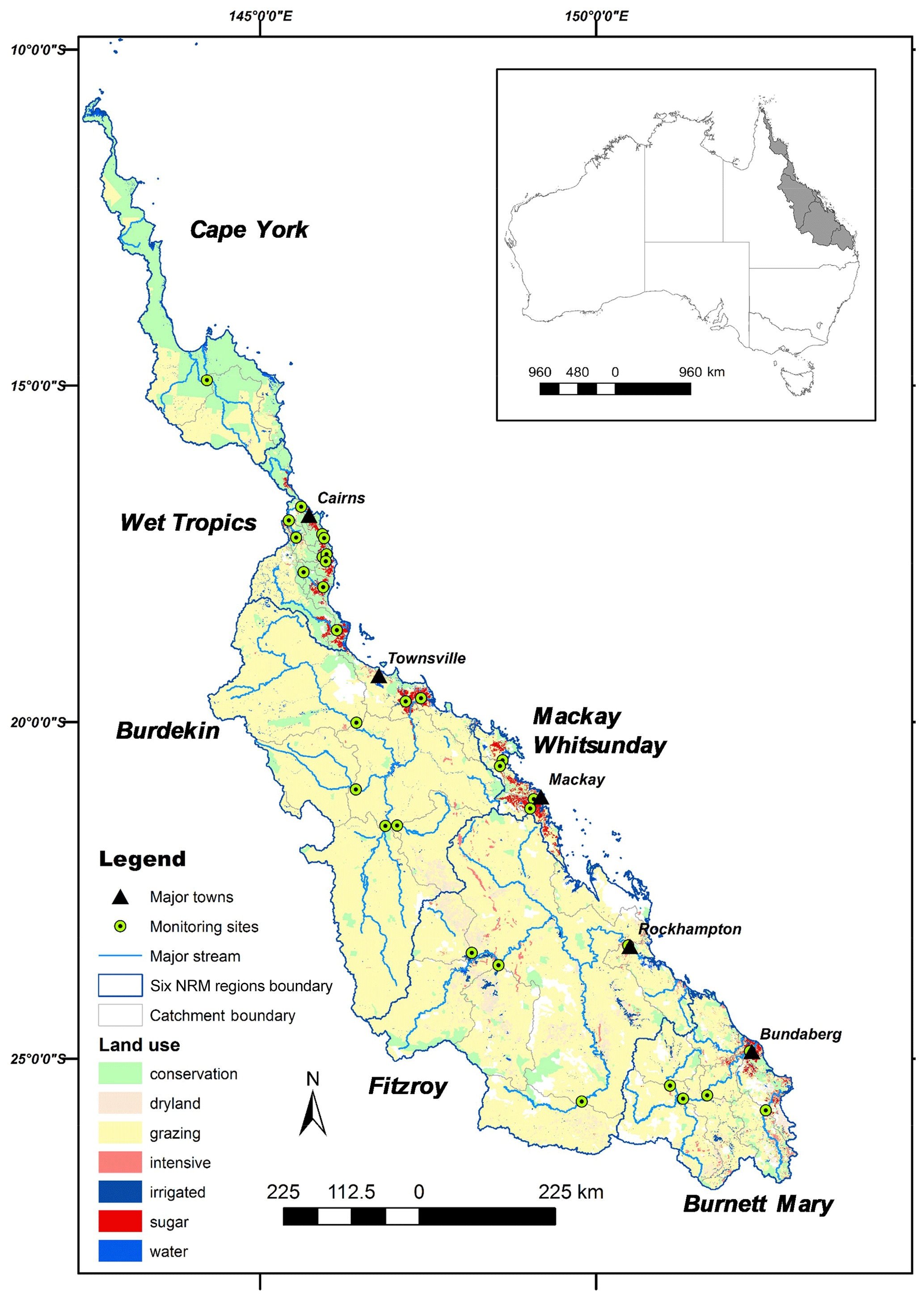
Figure 1The Great Barrier Reef (GBR) catchments, monitoring sites, land uses and the six natural resource management (NRM) regions. Land uses have the following characteristics: (1) conservation (forest, woodland, savannah, etc., for conservation purposes), (2) dryland (rainfed agriculture, including cereals but excluding grazing and sugar cane), (3) grazing (primarily cattle grazing of native and introduced vegetation), (4) intensive (urban areas, roads, etc.); (5) irrigated (irrigated cropping, excluding sugar cane); (6) sugar (rainfed and irrigated sugar cane) and (7) water (water bodies, including lake, river and marsh/wetland).

Figure 2Spatial information of the GBR catchments northeastern Australia. (a) Site locations showing two groups based on the clustering analysis of spatial variability in time-averaged water quality (Liu et al., 2018). (b) Topographic elevation (250 m resolution; Geoscience Australia, 2008). (c) Annual average rainfall (Atkinson et al., 2008, 2012). (d) Updated Köppen–Geiger climate zone classification (Peel et al., 2007).
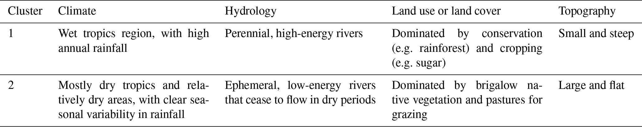
Table 1Summary of differences in landscape characteristics between the two clusters of sites (Liu et al., 2018).
2.1 Study area
The GBR catchments, situated in northeastern Australia (Fig. 1), consist of six natural resource management regions whose streams and rivers discharge into the Great Barrier Reef lagoon. These catchments cover a 437 354 km2, approximately a quarter of the state of Queensland, and exhibit significant diversity in climatic, geological and topographical landscape characteristics, as well as in land use and land management (Bartley et al., 2018; Gilbert and Brodie, 2001). The GBR catchments range from small, steep, high-energy streams in the wet tropics, which are dominated by sugarcane crops and rainforest, to large inland catchments used for savannah grazing and crops (e.g. grain) and with extensive low-energy floodplains in the dry tropics (Table 1; Davis et al., 2017; Koci et al., 2019; McKergow et al., 2005a). Spatial and temporal variations in rainfall in the GBR catchments are a major cause of the diversity in land use patterns. Annual rainfall ranges from less than 500 mm in the southwest to more than 8000 mm in the northeast (Fig. 2c; Davis et al., 2017; Kuhnert et al., 2009). Distinct wet (November to April) and dry (May to October) seasons result in high seasonal variation in runoff, and the El Niño–Southern Oscillation (ENSO) leads to high interannual variability (Day and McKeon, 2018). In the dry tropics, a few large events in the wet season contribute the majority of annual runoff, and constant low flow dominates during the dry season (Jarihani et al., 2017).
A total of 32 sites within the GBR catchments were selected as case study catchments (Fig. 1 and Table S1 in the Supplement). Previous multivariate analysis of the patterns of time-averaged concentrations indicated that there were two groups of sites (Table 1 and Fig. 2a). We found that differences in geographic and/or hydroclimatic catchment characteristics (Fig. 2b–d) are the key factors that distinguished the two clusters of sites (e.g. small wet areas, i.e. cluster 1, near the coast where topography, or orography, plays an important role in rainfall generation; Liu et al., 2018). Such geographic differences also lead to more dispersed sites in the drier area (cluster 2).
2.2 Data collection and preparation
2.2.1 Water quality data
The nine studied constituents were total suspended solids (TSSs), particulate nitrogen (PN), oxidised nitrogen (NOx), ammonium nitrogen (NH4), dissolved organic nitrogen (DON), filterable reactive phosphorus (FRP), dissolved organic phosphorus (DOP), particulate phosphorus (PP), and electrical conductivity (EC). Water quality monitoring data collected for the 32 GBR catchments over the 11-year period of 2006 to 2016 were obtained from the loads monitoring programme (Turner et al., 2012). This data set contained both high-frequency event-based samples (e.g. daily or every few hours by automatic samplers) that were taken during runoff events and grab samples (e.g. monthly) that were taken under baseflow conditions (Orr et al., 2014; Waters and Packett, 2007). As EC data from the loads monitoring programme were limited, we extracted additional EC data from the Water Monitoring Information Portal provided by the Department of Natural Resources, Mines and Energy of Queensland (DNRME, 2016) to complement the loads monitoring programme records.
2.2.2 Event mean concentration
We extracted continuous discharge records for each site from the Water Monitoring Information Portal (DNRME, 2016) to identify individual runoff events. An automated hydrograph analysis tool – HydRun (Tang and Carey, 2017) – was used to delineate runoff events. This approach allowed us to extract runoff event on the baseflow-free hydrograph by specifying a set of parameters (e.g. β filter coefficient – ReTh difference between two flows to set the local minima for event extraction). This toolbox directly returned the start and end points of an event, thereby avoiding time-consuming and subjective inconsistent outcomes. The key parameters used for the HydRun toolbox are provided in Table S2 in the Supplement, and an example hydrograph output is provided in Fig. S1. These parameters are determined based on recommended values from the literature (Garzon-Garcia et al., 2016; Ladson et al., 2013; Zhang et al., 2017) and a manual review of all event hydrographs ensured overall consistency. The event mean concentration (EMC) was then calculated for each event that had at least two samples on each of the rising and falling limbs of the hydrograph. Thus, for each EMC, a minimum of four samples was achieved, which is above the standard (three samples per event) set by Bartley et al. (2012). On average, there were 14 samples per event across the nine constituents (ranging from 12 for DOP to 16 for EC; Table S3 in the Supplement). This ensured that the water quality dynamics over a runoff event were reasonably well captured and that the derived EMCs were reliable (Waters and Packett, 2007). For each event, the EMC of a constituent was calculated as the total load per unit flow volume within the event using the following (Bartley et al., 2012):
where n is the total number of samples for a given event, cj is concentration of the jth sample, and and are the intersample mean discharge and time interval between jth and (j+1)th samples. The concentrations at the start and end of the event (c0 and cn+1) are assumed to be the averaged value for samples during baseflow (with baseflow identified in the previous section). The EMCs were essentially flow-weighted mean concentrations over individual runoff events, which allowed the comparison of water quality across catchments with contrasting flow regimes (e.g. two clusters of sites in Fig. 2; Cooke et al., 2000; Richards and Baker, 1993). A total of 1412 events was identified across the 32 sites, and depending on data availability, EMCs were calculated for between 21 % (DOP) and 43 % (TSS) of these identified runoff events (Table S2).
The derived EMCs (i.e. rather than the individual water quality samples) were Box–Cox transformed to improve the symmetry of the response variable (Box and Cox, 1964). The normalisation of the predictand is necessary to facilitate the fitting process and fulfil the statistical assumption of our model. This is because we use a Bayesian linear regression with the response variable sampled from a normal distribution (Sect. 2.3.1; Atkinson, 2021; Castillo et al., 2015; Hoeting et al., 2002). The site-level Box–Cox transformation parameter λ for each constituent was first identified, using the car package in R (Fox et al., 2012; R Core Team, 2013). Then, for each constituent, the average λ from the 32 sites was used to transform all available EMCs for that specific constituent. This ensured that an identical transformation parameter was applied across the different sites for each constituent (Guo et al., 2019).
Table 2Explanatory variables and their data sources.
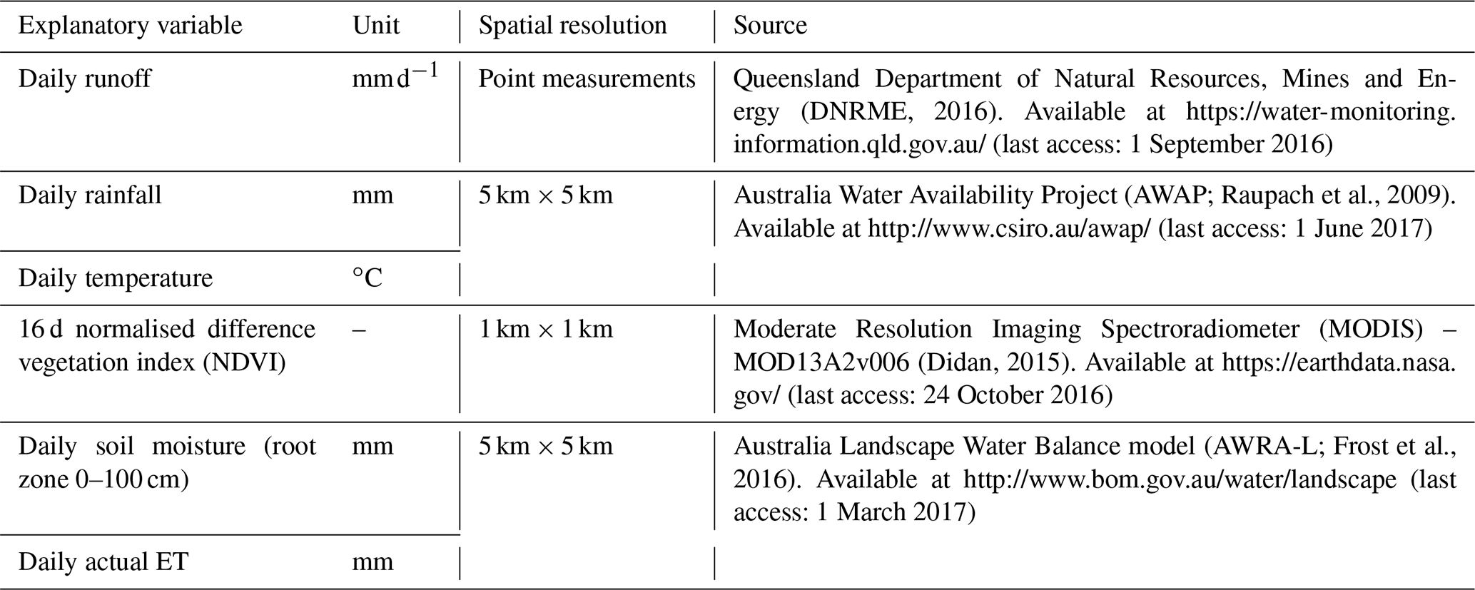
The term ET refers to evapotranspiration.
2.2.3 Explanatory variables
This study investigated the effect of various hydrologic, climatic and vegetation cover characteristics for different events. These characteristics included runoff, catchment root zone soil moisture, actual evapotranspiration rainfall, air temperature and vegetation cover. The continuous streamflow monitoring data, gridded weather and climatic products and remotely sensed imagery were used to derive catchment average conditions for each event (Table 2).
Table 3The three groups of event characteristics and the averaging method.
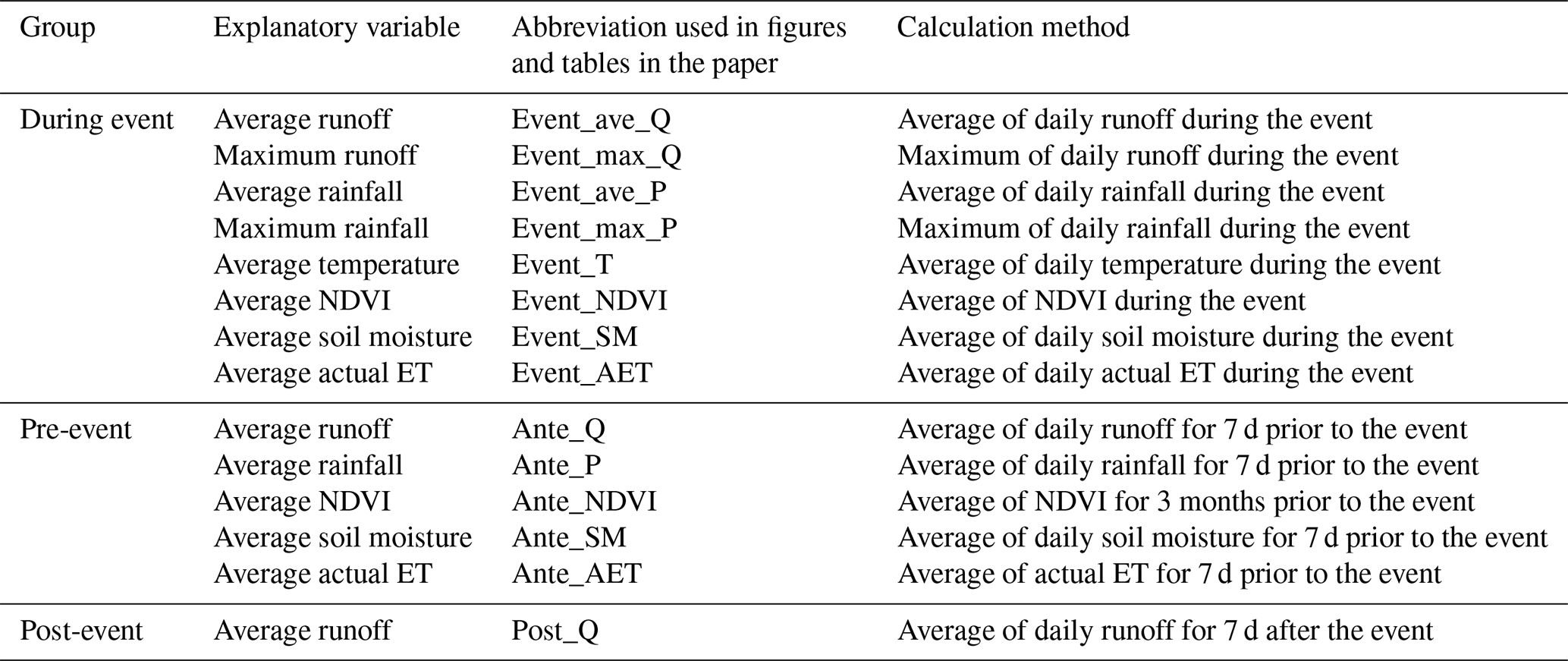
Note: Q – runoff; P – rainfall; T – temperature; NDVI – normalised difference vegetation index; SM – root zone soil moisture; ET – evapotranspiration.
For individual runoff events identified in the previous section, three groups of event characteristics were prepared, characterising pre-event, during-event and post-event conditions (Table 3). Except for runoff, data for all explanatory variables were first extracted from gridded data using catchment boundaries were delineated using the Geofabric (Australian Hydrological Geospatial Fabric) tool provided by the Australian Bureau of Meteorology (Atkinson et al., 2008; Fig. 1). The catchment-average time series data were then averaged over the specific time window related to the event (Table 3).
The explanatory variables in the during-event conditions were averaged over the duration of the event. For the pre-event and post-event conditions, the 7 d prior to and after the event were used as the time window (except NDVI). The 7 d period was the median of the time of concentration (i.e. the time for runoff to travel from the most remote point of the catchment to the monitoring site) across all catchments. These were estimated from catchment topography using the Bransby–William's equation, following its wide application in Australian catchments for flood estimation (Pilgrim et al., 1987). The ground cover was quantified by NDVI, an indicator of the biophysical condition of the vegetation canopy (Griffith et al., 2002). Previous studies have also shown that there is a time lag between water availability and a change in ground cover, which is typically 3 months for Australian catchments (De Keersmaecker et al., 2015). Therefore, to represent the pre-event ground cover condition, we averaged all available NDVI measurements for 3 months prior to an event. The runoff after the event (7 d) was also included as an indicator of catchment wetness at the end of the event to assess if the hydrologic condition towards the end of an event influences the temporal variation in water quality.
Similar to the EMCs, all the explanatory variables were Box–Cox transformed, following the procedure described in Sect. 2.2.2. In addition, prior to the analyses, both transformed EMCs and explanatory variables were standardised to a mean of 0 and standard deviation of 1. As such, the magnitude of a coefficient indicates the effect of each predictor relative to other predictors (Wan et al., 2014). The cross-correlation (non-parametric Spearman's rank correlation coefficient) of all transformed predictors is provided in Fig. S2 in the Supplement. Some of the variables are proxies for the same process, and thus, some paired predictors are highly correlated (e.g. pre-event NDVI and during-event NDVI with Spearman's ρ = 0.97). Freckleton (2011) highlighted that, when applying the model averaging approach, it is not safe to simply exclude correlated variables without due consideration of their likely independent effects. In our case, the high correlation among predictors mainly comes from time lag effects between predictors (e.g. pre-event, during event and post-event). The relative importance of these predictors provides a strong management indication for future water quality management strategies. Therefore, we have not removed any correlated predictors in this analysis. It is likely that different model structures result in similar predictive performance (discussed in the analysis of the results, i.e. Sect. 3.1).

Figure 3Analyses steps – the detailed methods used in the hierarchical modelling framework and model prediction and evaluation are in the following sections.
2.3 Modelling – driver identification and water quality prediction using multi-model inference
The statistical analysis and modelling followed several steps (Fig. 3). The Bayesian modelling framework was applied to catchments in clusters 1 and 2 separately. There are strong practical merits in handling the clusters separately. Previous results from clustering analyses on spatial patterns of water quality and catchment characteristics were highly correlated and the two clusters had quite different key explanatory variables (Liu et al., 2018). If all the sites were pooled into the same analysis, it would make it more difficult to identify a universal set of key explanatory variables that represent both clusters and likely increase the uncertainty of the coefficients too. The analysis would identify the same key factors identified for the two different clusters. It is important to consider and model these clusters separately so that we can better inform how water quality can be managed in these separate environmental conditions.
2.3.1 Bayesian variable selection
To investigate the relative importance of individual predictors, an indicator Bayesian variable selection method was used, and it is called the Gibbs variable selection (GVS; George and McCulloch, 1993). An auxiliary inclusion variable In (Eq. 2) for each predictor was introduced to indicate whether that predictor was in or out of an individual iteration of the hierarchical modelling structure.
In was modelled at the top level of the hierarchy, which enabled the use of identical model structures (i.e. combination of predictors) across different sites. The overarching hierarchical modelling framework was defined as follows:
The data-level model (Eq. 3) assumed that the EMC of a particular constituent (e.g. one of TSS, NOx, EC, etc.) at ith time step in the jth subcatchment, yi,j, followed a normal distribution (denoted as N(•)), with mean μi,j and a global standard deviation σ. The mean value, μi,j was modelled as the observed site-level-averaged EMC plus , with the latter term being defined as the deviation from this averaged value (Eq. 4; Guo et al., 2019). The deviation term incorporated the site-level-observed standard deviation , making Δi,j a standardised measure that could be compared across sites. Δi,j was further modelled as a linear additive function (Eq. 5) of all candidate predictors xn in n = 1, 2,…, N = 14 (e.g. event average runoff, rainfall and NDVI). Consequently, Δi,j was defined as the temporal variability in water quality and was the quantity of interest. The effect size (θn,j) of individual predictors was another latent variable used in the GVS and was estimated as the product of In and the regression coefficient βn,j (Eq. 6), such that θn,j was either βn,j (In=1) or 0 (In=0).
2.3.2 Hierarchical prior specification and Bayesian inference of key drivers
Bayesian inference required specification of prior distributions for each model parameter. We used a hierarchical conditional prior specification for predictor coefficients, allowing the site-specific parameter values that describe the effects of each of the temporal predictors () to be exchangeable between sites (O'Hara and Sillanpää, 2009; Webb and King, 2009). The detail specification of priors for each model parameter can be found in the Supplement. In addition, to identify key drivers affecting temporal changes in water quality, the posterior inclusion probability (); Eq. A8 in the Supplement) of each predictor was used to compare the relative importance of individual predictors (i.e. how often the nth predictor was in the model).
2.3.3 Prediction from multi-model inference
We used Bayesian model averaging to generate an ensemble of predictions of temporal variation in EMC for individual constituents (Eq. 7). The average posterior distribution of a quantity of interest (i.e. temporal variability in EMC) was generated using the parameters (e.g. ) sampled from the posterior distribution to simulate EMC values using the specific model, which is defined as follows:
where is the posterior distribution of a vector of (prediction) derived from model Mx, and P(Mk|y) is the posterior model probability (PMP; Eq. A8 in the Supplement; O'Hara and Sillanpää, 2009).
2.3.4 Model evaluation and implementation
The proposed modelling framework was applied to the two clusters of sites independently. This allowed an investigation of whether the spatial heterogeneity in catchment landscapes led to differences in the key factors controlling temporal variation in water quality. The key drivers were determined as the predictors with a PIP above 0.8 (i.e. over 80 % of the models included these predictors).
To further understand the reliability and robustness of the BMA framework, the consistency of the posterior inclusion probability of individual predictors was investigated by resampling subsets of the observations multiple times (Kohavi, 1995). For each cluster, 80 % of events within one site were first randomly selected, and the posterior inclusion probability for this subset of observations was estimated. This was repeated 1000 times to produce a distribution of posterior inclusion probabilities for individual predictors, which was then used to assess the uncertainty in the posterior inclusion probability.
An ensemble of the averaged prediction in temporal variability of each event was obtained from each iteration of parameter updating, using Markov chain Monte Carlo (MCMC). The model fit was evaluated using the Nash–Sutcliffe efficiency (NSE; Nash and Sutcliffe, 1970) between the observed temporal variability and the median of ensemble predictions derived from the BMA (Eq. 7). The NSE was calculated at both the cluster levels and site levels. The model residuals were also checked for normality and heteroscedasticity (i.e. relationship between the residual and predictors). In addition, model performance was evaluated by providing the 50 % and 95 % credible interval (CI) of each prediction.
To compare the relative importance of the predictors that have been widely used in the existing literature (i.e. runoff and rainfall) and other predictors (e.g. soil moisture, temperature, evapotranspiration and vegetation cover), the modelling framework was recalibrated using only the rainfall- and/or runoff-related predictors (including all pre-, during- and post-event predictors). This estimated the degree of improvement in the model's explanatory power with the inclusion of environmental variables, such as catchment wetness and ground vegetation cover conditions.
The hierarchical modelling framework was implemented in JAGS (Plummer, 2013a), using the package rjags in R (Plummer, 2013b; R Core Team, 2013), which enabled both the estimation of parameter values from prior distributions with MCMC and the generation of model-averaged predictions. The MCMC sampling had three parallel chains with 25 000 iterations for each chain. The first 5000 iterations were discarded as a burn-in period to allow convergence of the Markov chains, resulting in 60 000 values to estimate the posterior distribution for each model parameter and make model predictions.
3.1 Key drivers of temporal variability in water quality
The three key measures that were used to quantify the effect of individual predictors are (1) estimates of posterior inclusion probability (PIP), which quantifies relative importance of individual predictors; (2) posterior model probability (PMP), which estimates differences in plausible model structures; and (3) posterior distributions of coefficients for the key drivers (i.e. effect size; e.g. in Eq. 6), which measures direction and magnitude of the effect of key predictors on water quality temporal variability.
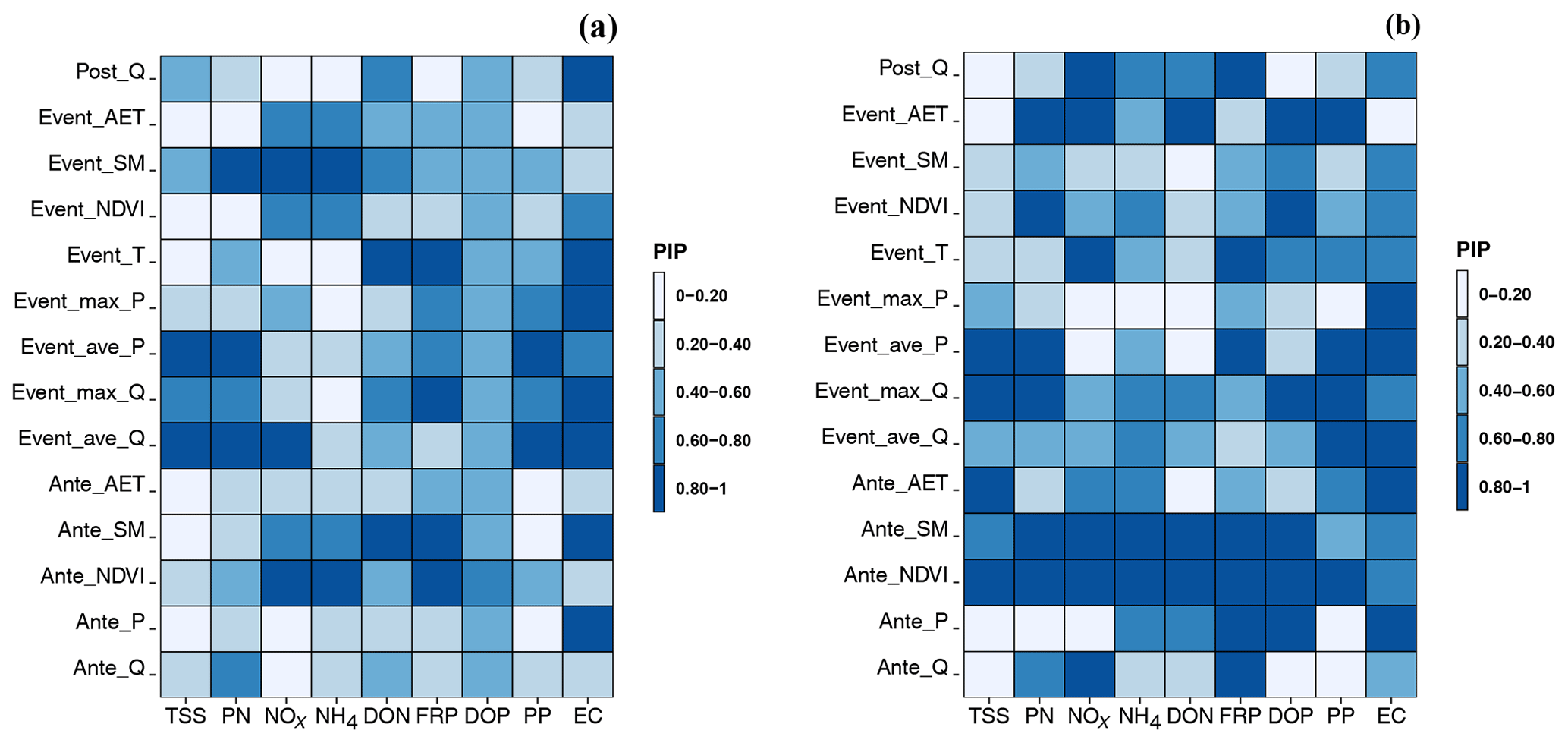
Figure 4Posterior inclusion probability (PIP) of each candidate predictor for (a) cluster 1 (wet) catchments and (b) cluster 2 (dry) catchments. Dark blue refers to high PIP, and light blue refers to low PIP. The definitions of the abbreviations of each predictor on the y axes are given in Table 3.
Posterior inclusion probability (Fig. 4 and Table S3 in Supplement) from the Bayesian modelling results indicated that, in general, antecedent vegetation condition and antecedent soil moisture were key factors in explaining temporal variation in water quality, especially for cluster 2 (warmer and drier) sites. Catchment runoff and rainfall were the second most important group of factors, especially for particulate pollutants (TSS, PN and PP; clusters 1 and 2) and salinity. In addition, the three groups of predictors (pre-, during and post-event) showed varying effects among the constituents. With regard to during-event conditions, event average runoff (Event_ave_Q), event maximum runoff (Event_max_Q) and event average rainfall (Event_ave_P) were three important factors with relatively high PIP. In contrast, among pre-event conditions, antecedent NDVI (Ante_NDVI) and antecedent soil moisture (Ante_SM) were driving factors for the majority of the constituents. Post-event runoff (Post_Q) only affected a few constituents (e.g. on NOx and FRP for cluster 2) compared with the other two groups of predictors. Overall, there were notable differences in the important predictors for clusters 1 and 2, and more important predictors were found for the cluster 2 sites.
It is also worth noting that strong correlations between predictors does not necessary mean that the posterior inclusion probability of these factors is similar (e.g. 1.00 and 0.34 for pre-event NDVI and event NDVI, respectively, for DON in cluster 2). The BMA can handle the collinearity by shrinking the posterior distribution of inclusion probability of one of the correlated variables towards zero (Nakagawa and Freckleton, 2011; Posch et al., 2020; Walker, 2019). This shrinkage effect leads to a lower posterior probability of a more complex model that includes correlated variables because each extra predictor dilutes the prior density of the existing predictor that it correlates with. Such a complex model is unlikely to be selected unless the loss in posterior probability can be outweighed by the gain in achieving a higher likelihood (Daoud, 2017; Hinne et al., 2020; Kruschke, 2014).
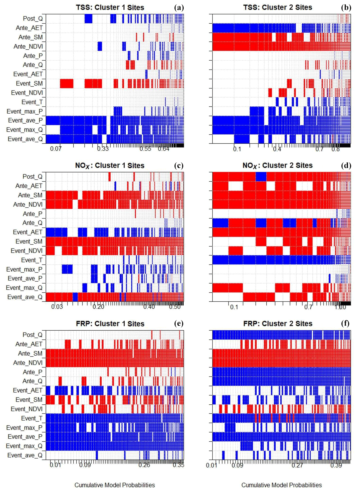
Figure 5Comparison of BMA model coefficients and cumulative model probabilities (only the first 100 models ranked according to the highest probability are shown) between cluster 1 (wet – a, c, e) and cluster 2 (dry – b, d, f) sites for (a) TSS, (b) NOx and (c) FRP. Each column in the heat map represents the one specific model (ranked from the highest model probability from left to right), and the width of the column is normalised by the posterior model probability (i.e. the widest columns indicate models with the largest increase in probability compared to the next most probable model). The colour indicates the direction of the coefficients; red is negative, and blue is positive. The coefficient value was averaged across the posterior median value of the site-specific coefficient within each cluster (effect size, θn,j, in Eq. 6). The definitions of the abbreviations of each predictor on the y axes are given in Table 3.
Results from here on will focus mainly on TSS, NOx and FRP due to their impacts on the marine receiving environment. Results for the other six constituents are in the Supplement. Figure 5 shows the posterior model probabilities for TSS, NOx and FRP for the 100 models with highest PMP (Figs. S3 and S4 in the Supplement show other constituents). Red indicates a negative influence and blue a positive influence. The difference in PIP between the two clusters resulted in quite different plausible model structures (models with relatively high posterior model probability). A stand-out difference between the results for the two clusters was antecedent vegetation cover condition (Ante_NDVI), which tended to be a more important predictor of TSS for cluster 2 than for cluster 1 (Fig. 5a). In addition, the plausible models for cluster 2 were generally more complex (with a larger number of predictors), except for DOP and EC (Figs. B3 and B4).

Figure 6Distribution of median of site-level coefficients for all plausible models in BMA between cluster 1 (wet – a, c, e) and cluster 2 (dry – b, d, f) sites for (a) TSS, (b) NOx and (c) FRP. Only predictors with PIP >0.8 are included. For each specific model structure, the coefficient value of a predictor was the median of the site-specific coefficient across all sites (effect size, θn,j, in Eq. 6). The distribution of this value thus represents the probability of the model (PMP) and the variability in the same predictor across different sites. Black dots show the median, grey vertical lines show the 95 % CI, and blue coloured vertical lines show the 50 % CI. The definitions of the abbreviations of each predictor on x axes are given in Table 3.
The distribution of posterior model coefficients for the key predictors (Figs. 6, B5 and B6) further demonstrated that the key drivers of temporal variability in water quality vary between catchments and between constituents. During-event runoff and rainfall tended to have a positive effect on sediment and particulate constituents and a negative effect on NOx and EC. In addition, there was strong negative effect of antecedent vegetation condition on the majority of the constituents.
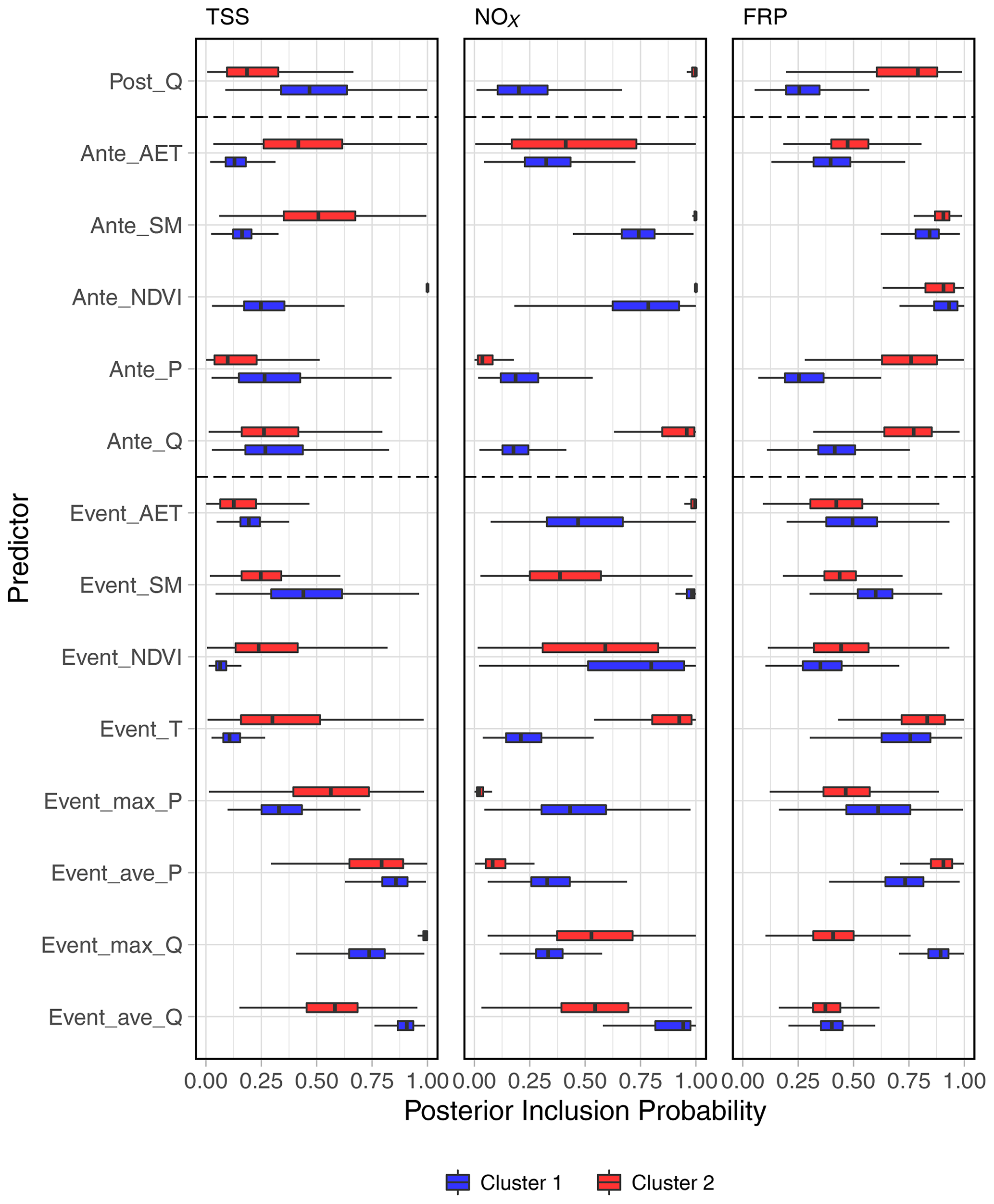
Figure 7The comparisons of the distribution of posterior inclusion probabilities of the individual predictors derived from 1000 subsampled BMA runs. The boxes are the interquartile ranges (IQRs; 25th to 75th percentile), and the whiskers are the ranges between the 1.5 IQR of the lower quartile and 1.5 IQR of the higher quartile. The vertical bar is the median. Blue shows cluster 1 (wet) catchments, and red shows cluster 2 (dry) catchments. The definitions of the abbreviations of each predictor on y axes are given in Table 3.
The uncertainty in PIP, derived from 1000 subsampled BMA runs (Figs. 7, B7 and B8) highlighted that the BMA results were robust for most constituents, except for EC (Fig. S7c in the Supplement). BMA tends to identify important predictors and is less sensitive to the input data, which is evidenced by the relatively narrow range of interquartile ranges (IQRs), when PIP for a specific predictor is large (e.g. antecedent soil moisture for FRP in Fig. 7). It is also worth noting that large uncertainty in the PIP for EC was observed, indicating the BMA results were sensitive to the observations of EC. This might be related to data availability, which is further discussed in Sect. 4.2.

Figure 8Performance of the BMA models of the temporal variability of three constituents across 32 sites, represented by prediction intervals from BMA and observed Box–Cox EMC across two clusters of sites for (a, b) TSS, (c, d) NOx and (e, f) FRP. Each bar shows a single event, and all events at all sites in the cluster are included. The NSE values were calculated based on median predictions. Black dots show prediction median, and grey vertical lines show the 95 % CI. Coloured vertical lines show the 50 % CI, and blue is cluster 1 (wet) catchments, and red is cluster 2 (dry) catchments. Dashed black lines are the 1:1 relationship.
3.2 Predictive performance
Moderate levels of temporal variability were explained by the BMA framework for the two independent clusters of sites (Figs. 8, S9 and S10 in the Supplement). At the cluster level, the NSE ranged from 0.04 (DOP) to 0.68 (EC) and from 0.34 (NH4) to 0.64 (NOx) for clusters 1 and 2 (full model columns in Table S6 in the Supplement), respectively. The comparison of the modelling performance (posterior median of BMA prediction) showed that the modelling framework performed better on the cluster 2 sites than cluster 1 (Fig. 8; red; 50 % prediction CI – cluster 2), except for NH4 and EC (not shown). This was reflected in a better match to the 1:1 line within the 90 % prediction CI for cluster 2 catchments. According to model performance criteria recommended by Moriasi et al. (2015), model performance is satisfactory (Table S7 in the Supplement), especially for the cluster 2 models. Generally, low NSE is acceptable for modelling nutrients and sediment compared to hydrology. It is also worth noting that, in contrast to the models developed here, most of the water quality models evaluated in Moriasi et al. (2015) are process-based models and focus on individual catchments.
It is also worth noting that the prediction interval for EC (Fig. S10c) was much wider than the rest of the constituents. Similar results were found in the site-level performance, with the average site-level NSE (Fig. S11 in the Supplement) for cluster 2 models typically higher than for cluster 1. The site-specific performance varied across sites, with the largest variation in EC (NSE for the cluster 2 result ranged from approximately 0.20 to 0.90). The modelling performance of DOP in the cluster 1 sites was poor (NSE = 0.04); all candidate covariates had low predictive power, resulting in the poor mixing of chains of the inclusion variable In (i.e. posterior In was around 0.5). The model residuals were normally distributed (Fig. S12 in the Supplement), and there was no clear heteroscedasticity within the residuals (Figs. S13 to S21 in the Supplement).
Table S6 (Supplement) compares the model performance using rainfall- and/or runoff-related predictors only and all candidate predictors (full model). A large increase in NSE was found for most dissolved nutrient species (e.g. NOx, NH4, DON, FRP and DOP) for the full model. Notably, for NH4 in cluster 1, factors other than rainfall and runoff explained almost all the variability that could be captured by the BMA.
4.1 Factors influencing temporal variability in stream water quality
4.1.1 Runoff and rainfall
Our results demonstrated that runoff and rainfall were important factors in explaining the temporal dynamics of particulate pollutants (i.e. TSS, PN and PP) and dissolved species (e.g. NOx, DOP and EC) in the GBR catchments. These results align with the findings of previous studies that have used these variables to understand changes in water quality over time (Beiter et al., 2020; McKergow et al., 2003; Schwarz et al., 2006).
Hydrologic and climatic variables (i.e. rainfall and runoff) showed distinct effects on different constituents and different groups of catchments. The positive effect of event runoff and rainfall on sediment and particulate nutrients (i.e. PN and PP) revealed their underlying impacts on pollutant mobilisation and transport processes in catchments (Hirsch et al., 2010; Lintern et al., 2018b; Musolff et al., 2015). In contrast, there were negative effects of during-event runoff on NOx (cluster 1), DOP (cluster 2) and EC (both clusters). For NOx and EC, this was most likely caused by hydrological transport processes; these constituents tend to be transported to receiving rivers via subsurface flows (Kratz et al., 1997; McKergow et al., 2003). For events with relatively low surface runoff, higher NOx and EC event concentrations could be expected in these catchments (Clow and Sueker, 2000; Skoulikidis et al., 2006). In addition, for DOP, in-stream biogeochemical cycling was likely to have caused the negative effect of event runoff. The events with low runoff, coupled with high temperatures (positive effect of event temperature for DOP cluster 2; Fig. S4a) may relate to increases in the rate of P releases from organic forms at higher temperatures (Verheyen et al., 2015).
Post-event runoff (Post_Q) showed effects on specific constituents (e.g. NOx, FRP and EC). There are two alternative reasons that might explain this. First, high post-event runoff may be an indicator of large baseflow contribution during the events (Cuomo and Guida, 2016). Therefore, as discussed in the above paragraph, constituents that can be transported through subsurface flows tend to be influenced by amount of runoff post-event. Alternatively, it was significantly and positively correlated with other event characteristics and catchment biophysical conditions (e.g. vegetation cover; Fig. S2). Together, these intercorrelated factors could have influenced pollutant source, mobilisation and delivery (see discussions below; Granger et al., 2010; Lintern et al., 2018a).
4.1.2 Vegetation cover
Vegetation cover was another driving factor that was found to have influenced water quality dynamics; antecedent NDVI (Ante_NDVI) was included in the plausible models more frequently than event NDVI. The negative effect of antecedent NDVI on particulate and dissolved nutrients (except for DOP) was in line with previous studies that have found that NDVI was negatively correlated with these constituent concentrations in streams (Griffith et al., 2002; Masocha et al., 2017). An explanation for these results could be that high vegetation groundcover tended to stabilise the surface soil and reduce sediment losses by erosion (Meyer et al., 1997; Singh et al., 2008). In addition, vegetation nutrient assimilation and retention processes consumed nutrients in sediment and waterbodies, and these processes peaked in spring and early summer, typically before the wet season in the GBR catchments (Tabacchi et al., 2000; Vymazal, 2007).
The effect of antecedent NDVI varied among groups of constituents in clusters 1 and 2. Specifically, it was a key predictor for NOx, NH4 and FRP for cluster 1 and almost all constituents for cluster 2. This can be explained by the contrasting landscapes and climate of these two regions (Liu et al., 2018). In the dense, vegetation-covered catchments in cluster 1 (i.e. the sites in the wet tropics), dissolved inorganic nutrient losses were likely due to more fertile soils (e.g. application of fertiliser on sugarcane) during the growing season (McKergow et al., 2005a). Furthermore, denser natural vegetation cover (e.g. riparian vegetation and forest) could increase plant uptake and assimilation of dissolved nutrients compared to the sparse vegetation cover in the dry tropics (cluster 2) region. Conversely, among cluster 2 sites, vegetation coverage showed clear seasonal variation, which was linked closely to the seasonality in rainfall and grazing activity. Sediments and particulate pollutants were likely to be mobilised in grazed catchments (high rate of soil erosion) and delivered to streams via surface runoff (Neil et al., 2002; Turner et al., 2012). More importantly, high vegetation cover tended to mitigate mobilisation of pollutants through stabilising the surface soil and reducing sediment losses from erosion (Meyer et al., 1997; Singh et al., 2008).
4.1.3 Soil moisture and evapotranspiration
The results showed that soil moisture (SM) and actual evapotranspiration (AET) had a high impact on different constituents, particularly in the cluster 2 catchments (e.g. antecedent soil moisture – DON and EC; antecedent AET – TSS and EC). These two variables were intercorrelated and affect the hydrological cycle and vegetation cover (Correll, 1996). The results indicated that antecedent soil moisture had a negative effect on PN, NOx, NH4, DON, DOP and FRP. On one hand, this was expected as antecedent soil moisture was positively correlated with vegetation cover, and high soil moisture tends to reduce soil erosion and increase plant nutrient uptake. It may also be that soil water content affected soil microbial activity, influencing the biogeochemical processes in catchments, such as denitrification (Doran et al., 1988; Weier et al., 1993). The rate of denitrification was also enhanced under anoxic conditions, when soil moisture was high (Zhu et al., 2019). On the other hand, higher soil water can be associated with increased shallow subsurface flow and leaching of some constituents such as NOx (Zhu et al., 2018). This appears not to occur to a sufficient extent for it to override other impacts of soil moisture.
4.1.4 Temperature
Our results suggested that average event temperature (Event_T) had a positive effect on NOx, FRP and DOP. This may be attributed to the strong negative cross-correlation between temperature and event runoff and antecedent vegetation condition (Fig. S2). Rainfall during a warmer period might have been associated with less event runoff, resulting in higher event mean concentrations (Sect. 4.1.1). The effect of event temperature can be also attributed to the fact that the higher temperatures could lead to more recent mineralisation of nutrients, increasing readily transportable dissolved nutrient sources (Liu et al., 2017; Wang et al., 2020). Temperature is one controlling factor that affects pollution transformation (Barnard et al., 2005). For instance, temperature has a direct impact on the activity of microorganisms, which affects the intensity of biological processes such as denitrification (Wakelin et al., 2011). In addition, higher event temperature might be associated with higher pre-event temperature, resulting in poor groundcover, potentially lowering the dissolved nutrients losses through plant assimilation and/or uptake (Sect. 4.1.2; Muro et al., 2018).
4.2 Predicting temporal variations in water quality
The Bayesian modelling framework in this study provided a useful tool to assess in-stream water quality dynamics. The models were able to explain more temporal variation in NOx and EC than in other constituents. This is related to the sources and delivery processes of these two constituents. Anthropogenic inputs (e.g. agriculture) for NOx and large stores in groundwater together with limited geochemical transformation for EC (salts) suggested that temporal changes in event concentration could be well captured by the changes in catchment hydroclimatic and vegetation conditions. In addition, NOx and EC tend to be transported in subsurface flow pathways. The dynamics of catchment soil wetness and vegetation cover have been previously linked to hydrological interactions between surface and subsurface flows (Ursino et al., 2004). The incorporation of soil moisture and vegetation cover into the Bayesian modelling framework more readily allowed the description of the main ecohydrological processes of these two constituents.
In contrast, model performance for DOP was poor in cluster 1 catchments, which can be explained by two reasons. First, in the wet tropics catchments, DOP concentrations were generally stable, regardless of changes in flow, which can be explained by chemical exchange processes between water and sediment in stream (White et al., 1998). This means that the variability in DOP cannot be captured by the environmental variables considered here. Second, the poor performance might be attributed to the data set having fewer observations of DOP EMCs among cluster 1 sites. There were only 66 observations, compared to the next lowest number of 167 (EC) among other constituents in the cluster 1 catchments, which may not be sufficient to fully inform the model. This small sample size could have led to (1) poor mixing of MCMC chains for inclusion variables (Fig. S8a in the Supplement), where no predictors showed predictive power, and (2) the BMA failed to identify the plausible models, since none of the candidate models had enough predictive power to fit the data well (Guthke, 2017; Höge et al., 2019). Continuous DOP monitoring would be required to achieve a better understanding of the factors driving temporal variation in this constituent. Therefore, we did not infer any conclusions from the modelling results of DOP in cluster 1 due to the poor modelling performance.
The modelling performance in this study is generally higher than our previous studies (i.e. Guo et al. (2019, 2020)). This improved performance can be attributed to the following:
-
Differences in water quality monitoring data.
Rivers in Queensland are more event dominated; thus, we used event-based water quality data compared to our previous studies, which used monthly water quality data in Victoria. The uncertainty in event-based water quality samples has less impact on modelling performance because we considered the variability in streamflow when developing EMCs in this study (Chen et al., 2017; Lessels and Bishop, 2015; Letcher et al., 2002).
-
Differences in modelling methods.
Here, we used a model-averaging approach that considered model predictions from multiple candidate models, rather than a single model approach that was used our previous studies (Guo et al., 2020, 2019). This approach is a more robust approach to providing predictions because the predictions consider the model selection uncertainty (Höge et al., 2019; Raftery et al., 1997).
Statistical modelling in hydrology or water quality is affected by uncertainty, only some of which can be characterised within any particular modelling framework (Kavetski et al., 2006; Mantovan and Todini, 2006; Renard et al., 2010). The Bayesian modelling framework used in this study incorporated the uncertainties in model selection (between model), observations and model parameters (within model) directly into the model predictions (Steel, 2019). This is a more comprehensive characterisation than in studies where model structures are assumed a priori. Reporting of predictive uncertainty of temporal variations in water quality also provided valuable information on the confidence in the averaged predictions. In addition, as discussed in Sect. 2.3, due to strong practical and conceptual reasons, our modelling framework was applied to two clusters of sites separately. However, this method can be used anywhere, e.g. a single modelling framework for all sites. Thus, we are not making claims that there are always variables that will be important in such catchments. Our method is universal, but our results are not.
Nevertheless, limitations remain in the BMA approach which are important to understand. For example, for EC, there was a larger predictive uncertainty and larger uncertainty in posterior inclusion probability for each predictor from the robustness assessment than estimated in the fit to the complete data set. A limitation of BMA is that the posterior model probability could be sensitive to the specification of the parameter prior distribution (Fernandez et al., 2001). Specifying more informative priors on model parameters (i.e. inclusion variable In) would have the effect of restricting the set of candidate models (Rockey and Temple, 2016). Indeed, several studies have compared different predictive performances of different prior specification of BMA coefficients and found that the choice of prior matters (Bayarri et al., 2012; Liang et al., 2008). Future investigation of the sensitivity of prior distributions for BMA coefficients might achieve a reduction in predictive uncertainty and instability in posterior inclusion probabilities.
4.3 Management implications
The identification of key drivers of temporal variation in water quality can inform catchment water quality management. The results of this study showed that the effects of hydro-climatic drivers (e.g. rainfall and runoff) and vegetation cover varied among constituents and regions. This may allow funding bodies, such as government and regional natural resource management groups, to identify regions where land management and restoration would have a greater effect on mitigating sediments and nutrients export. The results suggested that, compared to wet catchments, maintaining vegetation ground cover in large dry grazed catchments (e.g. the Burdekin and Fitzroy catchments in cluster 2) before the wet seasons could be an effective way of reducing sediment losses via erosion processes. These results are consistent with current, improved land management practices across the GBR catchments (Brodie et al., 2012; Queensland Government, 2017). Management measures (e.g. establishment of wetlands, revegetation and/or rehabilitation of gullies and stabilisation of river banks) can reduce sediment losses from hillslope and gully erosions (Koci et al., 2020; Sherriff et al., 2016). In addition, catchment-specific management that accounts for temporal variation in catchment hydrological connectivity is required for the control of dissolved nutrients. Dominant flow pathways for dissolved nutrients can vary spatially and temporally. For example, subsurface flow in the wet tropics region have tended to transmit more dissolved nutrients because prolonged wet conditions lead to this region being more likely to be connected via lateral subsurface flow (Geng et al., 2017). The enhanced mobilisation of leached dissolved nutrients from intensive cropping (e.g. sugarcane) from perched groundwater should be targeted in these catchments (Melland et al., 2012). Management practices, such as conservation tillage, and adaptation of the 4R concept (right source, right rate, right time and right place) for fertiliser application may help to minimise dissolved nitrogen losses (Lintern et al., 2020; Snyder, 2017).
This study provides a data-driven understanding of key drivers influencing the temporal variation in water quality. A hierarchical Bayesian model averaging framework was used to identify the key environmental drivers and predict the water quality dynamics at multiple catchments. Results showed that the temporal dynamics of water quality can be predicted well using models considering the combined effects of hydroclimate and vegetation groundcover. The effects of key hydro-climatic and vegetation conditions varied among different constituents and across regions. This study reinforces the importance of vegetation cover management as one key management response, especially for large grazed catchments. Future investigation could involve the development of a spatio-temporal modelling framework to fully capture the water quality dynamics. More importantly, it has continued to be challenging to prioritise management practices and evaluate the effectiveness of the improved management interventions. Consequently, with more land management surveys and continuous water quality monitoring data available, an extended temporal or spatio-temporal modelling framework could potentially be used to assess if the success of the restoration measures.
Water quality data that supported this study are available upon request from the Great Barrier Reef Catchment loads monitoring programme (gbrevents@dsiti.qld.gov.au). Sources of explanatory variables are listed in Table 2.
The supplement related to this article is available online at: https://doi.org/10.5194/hess-25-2663-2021-supplement.
SL carried out data collation, performed the simulations and took the lead in writing the paper. DR, AWW, JAW, AL and DG contributed to the design of the research, interpretation of the results and supervision of the project. DW assisted with the data collation and provided critical feedback and helped shape the research, analysis and paper.
The authors declare that they have no conflict of interest.
This article is part of the special issue “Frontiers in the application of Bayesian approaches in water quality modelling”. It is a result of the EGU General Assembly 2020, 3–8 May 2020.
This study was supported by the Australian Research Council (grant no. LP140100495). The authors would like to acknowledge the efforts of the Queensland Department of Environment and Science, who provided the water quality monitoring data. The authors would also like to offer their sincere gratitude to Jie Jian for her assistance with the geospatial database compilation. Paul Leahy, Malcolm Watson, Ulrike Bende-Michl, Paul Wilson and Belinda Thompson are thanked for providing valuable advice in the preparation of this paper.
This research has been supported by the Australian Research Council (grant no. LP140100495).
This paper was edited by James E. Sample and reviewed by two anonymous referees.
Abbaspour, K. C., Rouholahnejad, E., Vaghefi, S., Srinivasan, R., Yang, H., and Kløve, B.: A continental-scale hydrology and water quality model for Europe: Calibration and uncertainty of a high-resolution large-scale SWAT model, J. Hydrol., 524, 733–752, 2015.
Abbott, M., Bathurst, J., Cunge, J., O'connell, P., and Rasmussen, J.: An introduction to the European Hydrological System—Systeme Hydrologique Europeen,“SHE”, 2: Structure of a physically-based, distributed modelling system, J. Hydrol., 87, 61–77, 1986.
Arnold, J. G. and Fohrer, N.: SWAT2000: current capabilities and research opportunities in applied watershed modelling, Hydrol. Process., 19, 563–572, 2005.
Atkinson, A. B.: The box-cox transformation: Review and extensions, Stat. Sci., 36, 239–255, 2021.
Atkinson, R., Power, R., Lemon, D., O'Hagan, R., Dovey, D., and Kinny, D.: The Australian Hydrological Geospatial Fabric–Development Methodology and Conceptual Architecture, Citeseer, 2008.
Barnard, R., Leadley, P. W., and Hungate, B. A.: Global change, nitrification, and denitrification: a review, Global Biogeochem. Cy., 19, GB1007, https://doi.org/10.1029/2004GB002282, 2005.
Bartley, R., Speirs, W. J., Ellis, T. W., and Waters, D. K.: A review of sediment and nutrient concentration data from Australia for use in catchment water quality models, Mar. Pollut. Bull., 65, 101–116, 2012.
Bartley, R., Thompson, C., Croke, J., Pietsch, T., Baker, B., Hughes, K., and Kinsey-Henderson, A.: Insights into the history and timing of post-European land use disturbance on sedimentation rates in catchments draining to the Great Barrier Reef, Mar. Pollut. Bull., 131, 530–546, 2018.
Bayarri, M. J., Berger, J. O., Forte, A., and García-Donato, G.: Criteria for Bayesian model choice with application to variable selection, Ann Statist., 40, 1550–1577, 2012.
Beiter, D., Weiler, M., and Blume, T.: Characterising hillslope–stream connectivity with a joint event analysis of stream and groundwater levels, Hydrol. Earth Syst. Sci., 24, 5713–5744, https://doi.org/10.5194/hess-24-5713-2020, 2020.
Bieger, K., Hörmann, G., and Fohrer, N.: Simulation of streamflow and sediment with the soil and water assessment tool in a data scarce catchment in the three Gorges region, China, J. Environ. Qual., 43, 37–45, 2014.
Box, G. E. and Cox, D. R.: An analysis of transformations, J. Roy. Stat. Soc. B Met., 26, 211–243, 1964.
Brevik, E. C., Fenton, T. E., and Lazari, A.: Soil electrical conductivity as a function of soil water content and implications for soil mapping, Precis. Agric., 7, 393–404, 2006.
Brodie, J. E., Kroon, F., Schaffelke, B., Wolanski, E., Lewis, S., Devlin, M., Bohnet, I., Bainbridge, Z., Waterhouse, J., and Davis, A.: Terrestrial pollutant runoff to the Great Barrier Reef: an update of issues, priorities and management responses, Mar. Pollut. Bull., 65, 81–100, 2012.
Castillo, I., Schmidt-Hieber, J., and Van der Vaart, A.: Bayesian linear regression with sparse priors, Ann Statist., 43, 1986–2018, 2015.
Chang, F.-J., Tsai, Y.-H., Chen, P.-A., Coynel, A., and Vachaud, G.: Modeling water quality in an urban river using hydrological factors–Data driven approaches, J. Environ. Manage., 151, 87–96, 2015.
Chen, L., Sun, C., Wang, G., Xie, H., and Shen, Z.: Event-based nonpoint source pollution prediction in a scarce data catchment, J. Hydrol., 552, 13–27, 2017.
Clow, D. W. and Sueker, J. K.: Relations between basin characteristics and stream water chemistry in alpine/subalpine basins in Rocky Mountain National Park, Colorado, Water Resour. Res., 36, 49–61, 2000.
Cooke, S. E., Ahmed, S. M., and MacAlpine, N.: Introductory guide to surface water quality monitoring in agriculture, Conservation and Development Branch, Alberta Agriculture, Food and Rural Development, Edmonton, 2000.
Correll, D.: Buffer zones and water quality protection: general principles, Buffer zones: Their processes and potential in water protection, September 1996, Harpenden, England, 7–20, 1996.
Cuomo, A. and Guida, D.: Using hydro-chemograph analyses to reveal runoff generation processes in a Mediterranean catchment, Hydrol. Process., 30, 4462–4476, 2016.
Daoud, J. I.: Multicollinearity and regression analysis, J. Phys.-Conf. Ser., 949, 012003, https://doi.org/10.1088/1742-6596/949/1/012009, 2017.
Davis, A. M., Pearson, R. G., Brodie, J. E., and Butler, B.: Review and conceptual models of agricultural impacts and water quality in waterways of the Great Barrier Reef catchment area, Mar. Freshwater Res., 68, 1–19, 2017.
Day, K. A. and McKeon, G. M.: An index of summer rainfall for Queensland's grazing lands, J. Appl. Meteorol. Clim., 57, 1623–1641, 2018.
De Keersmaecker, W., Lhermitte, S., Tits, L., Honnay, O., Somers, B., and Coppin, P.: A model quantifying global vegetation resistance and resilience to short-term climate anomalies and their relationship with vegetation cover, Global Ecol. Biogeogr., 24, 539–548, 2015.
de Mello, K., Valente, R. A., Randhir, T. O., dos Santos, A. C. A., and Vettorazzi, C. A.: Effects of land use and land cover on water quality of low-order streams in Southeastern Brazil: Watershed versus riparian zone, Catena, 167, 130–138, 2018.
Deletic, A. B. and Maksimovic, C.: Evaluation of water quality factors in storm runoff from paved areas, J. Environ. Eng., 124, 869–879, 1998.
Didan, K.: MOD13A2 MODIS/Terra Vegetation Indices 16-Day L3 Global 1km SIN Grid V006, NASA EOSDIS LP DAAC, https://doi.org/10.5067/MODIS/MOD13A2.006, 2015.
DNRME: available at: https://water-monitoring.information.qld.gov.au/ (last access: 1 September 2016), Department of Natural Resources, Mines and Energy of Queensland, Brisbane, 2016.
Doran, J., Mielke, L., and Stamatiadis, S.: Microbial activity and N cycling as regulated by soil water-filled pore space, 11th International Conference, Int. Soil Tillage Res. Orgo (ISTRO), Edinburgh, Scotland, 49–54, 1988.
Fernandez, C., Ley, E., and Steel, M. F.: Benchmark priors for Bayesian model averaging, J. Econometrics, 100, 381–427, 2001.
Filoso, S., Vallino, J., Hopkinson, C., Rastetter, E., and Claessens, L.: Modeling nitrogen transport in the Ipswich River Basin, Massachusetts, using a hydrological simulation program in FORTRAN (HSPF) 1, J. Am. Water Resour. As., 40, 1365–1384, https://doi.org/10.1111/j.1752-1688.2004.tb01592.x, 2004.
Fox, J., Weisberg, S., Adler, D., Bates, D., Baud-Bovy, G., Ellison, S., Firth, D., Friendly, M., Gorjanc, G., and Graves, S.: Package “car”, R Foundation for Statistical Computing, Vienna, 2012.
Francesconi, W., Srinivasan, R., Pérez-Miñana, E., Willcock, S. P., and Quintero, M.: Using the Soil and Water Assessment Tool (SWAT) to model ecosystem services: A systematic review, J. Hydrol., 535, 625–636, 2016.
Freckleton, R. P.: Dealing with collinearity in behavioural and ecological data: model averaging and the problems of measurement error, Behav. Ecol. Sociobiol., 65, 91–101, 2011.
Frost, A., Ramchurn, A., and Smith, A.: The Bureau's Operational AWRA Landscape (AWRA-L) Model, Bureau of Meteorology, Melbourne, 47, 2016.
Fu, B., Merritt, W. S., Croke, B. F., Weber, T., and Jakeman, A. J.: A review of catchment-scale water quality and erosion models and a synthesis of future prospects, Environ. Modell. Softw., 114, 75–97, 2019.
Garzon-Garcia, A., Wallace, R., Huggins, R., Turner, R. D., Smith, R., Orr, D., Ferguson, B., Gardiner, R., Thomson, B., and Warne, M.: Total suspended solids, nutrient and pesticide loads (2013–2014) for rivers that discharge to the Great Barrier Reef, Department of Science, Information Technology and Innovation, Brisbane, Australia, 2016.
Gelman, A., Stern, H. S., Carlin, J. B., Dunson, D. B., Vehtari, A., and Rubin, D. B.: Bayesian data analysis, Chapman and Hall/CRC, Florida, US, 2013.
Geng, X., Heiss, J. W., Michael, H. A., and Boufadel, M. C.: Subsurface flow and moisture dynamics in response to swash motions: Effects of beach hydraulic conductivity and capillarity, Water Resour. Res., 53, 10317–10335, 2017.
George, E. I. and McCulloch, R. E.: Variable selection via Gibbs sampling, J. Am. Stat. Assoc., 88, 881–889, 1993.
Geoscience Australia: GEODATA 9 second DEM and D8: digital elevation model version 3 and flow direction grid 2008, Bioregion Assessment Source Dataset, Geoscience Australia, Canberra, Australia, 2008.
Gilbert, M. and Brodie, J.: Population and major land use in the Great Barrier Reef catchment area spatial and temporal trends, Great Barrier Reef Marine Park Authority, Townsville, 2001.
Gorman, D., Russell, B. D., and Connell, S. D.: Land-to-sea connectivity: linking human-derived terrestrial subsidies to subtidal habitat change on open rocky coasts, Ecol. Appl., 19, 1114–1126, 2009.
Granger, S., Bol, R., Anthony, S., Owens, P., White, S., and Haygarth, P.: Towards a holistic classification of diffuse agricultural water pollution from intensively managed grasslands on heavy soils, Adv. Agron., 105, 83–115, 2010.
Griffith, J. A.: Geographic techniques and recent applications of remote sensing to landscape-water quality studies, Water Air Soil Poll., 138, 181–197, 2002.
Griffith, J. A., Martinko, E. A., Whistler, J. L., and Price, K. P.: Interrelationships among landscapes, NDVI, and stream water quality in the US Central Plains, Ecol. Appl., 12, 1702–1718, 2002.
Guo, D., Lintern, A., Webb, J. A., Ryu, D., Liu, S., Bende-Michl, U., Leahy, P., Wilson, P., and Western, A.: Key Factors Affecting Temporal Variability in Stream Water Quality, Water Resour. Res., 55, 112–129, 2019.
Guo, D., Lintern, A., Webb, J. A., Ryu, D., Bende-Michl, U., Liu, S., and Western, A. W.: A data-based predictive model for spatiotemporal variability in stream water quality, Hydrol. Earth Syst. Sci., 24, 827–847, https://doi.org/10.5194/hess-24-827-2020, 2020.
Guthke, A.: Defensible model complexity: A call for data-based and goal-oriented model choice, Groundwater, 55, 646–650, 2017.
Harris, G. P.: Biogeochemistry of nitrogen and phosphorus in Australian catchments, rivers and estuaries: effects of land use and flow regulation and comparisons with global patterns, Mar. Freshwater Res., 52, 139–149, 2001.
Hem, J. D.: Fluctuations in concentration of dissolved solids of some southwestern streams, Eos T. Am. Geophys. Un., 29, 80–84, 1948.
Hinne, M., Gronau, Q. F., van den Bergh, D., and Wagenmakers, E.-J.: A Conceptual Introduction to Bayesian Model Averaging, Advances in Methods and Practices in Psychological Science, 3, 200–215, 2020.
Hirsch, R. M., Moyer, D. L., and Archfield, S. A.: Weighted regressions on time, discharge, and season (WRTDS), with an application to Chesapeake Bay river inputs, J. Am. Water Resour. As., 46, 857–880, 2010.
Hoeting, J. A., Raftery, A. E., and Madigan, D.: Bayesian variable and transformation selection in linear regression, J. Comput. Graph. Stat., 11, 485–507, 2002.
Höge, M., Guthke, A., and Nowak, W.: The hydrologist's guide to Bayesian model selection, averaging and combination, J. Hydrol., 572, 96–107, 2019.
Howarth, R. W., Sharpley, A., and Walker, D.: Sources of nutrient pollution to coastal waters in the United States: Implications for achieving coastal water quality goals, Estuaries, 25, 656–676, 2002.
Jarihani, B., Sidle, R., Bartley, R., Roth, C., and Wilkinson, S.: Characterisation of hydrological response to rainfall at multi spatio-temporal scales in savannas of semi-arid Australia, Water, 9, 540, https://doi.org/10.3390/w9070540, 2017.
Jayakrishnan, R., Srinivasan, R., Santhi, C., and Arnold, J.: Advances in the application of the SWAT model for water resources management, Hydrol. Process., 19, 749–762, 2005.
Kasiviswanathan, K. and Sudheer, K.: Quantification of the predictive uncertainty of artificial neural network based river flow forecast models, Stoch. Env. Res. Risk A., 27, 137–146, 2013.
Kavetski, D., Kuczera, G., and Franks, S. W.: Bayesian analysis of input uncertainty in hydrological modeling: 1. Theory, Water Resour. Res., 42, W03407, https://doi.org/10.1029/2005WR004368, 2006.
Khan, U., Cook, F. J., Laugesen, R., Hasan, M. M., Plastow, K., Amirthanathan, G. E., Bari, M. A., and Tuteja, N. K.: Development of catchment water quality models within a realtime status and forecast system for the Great Barrier Reef, Environ. Modell. Softw., 132, 104790, https://doi.org/10.1016/j.envsoft.2020.104790, 2020.
Koci, J., Sidle, R. C., Jarihani, B., and Cashman, M. J.: Linking hydrological connectivity to gully erosion in savanna rangelands tributary to the Great Barrier Reef using Structure-from-Motion photogrammetry, Land Degrad. Dev., 31, 20–36, 2019.
Koci, J., Sidle, R. C., Kinsey-Henderson, A. E., Bartley, R., Wilkinson, S. N., Hawdon, A. A., Jarihani, B., Roth, C. H., and Hogarth, L.: Effect of reduced grazing pressure on sediment and nutrient yields in savanna rangeland streams draining to the Great Barrier Reef, J. Hydrol., 582, 124520, https://doi.org/10.1016/j.jhydrol.2019.124520, 2020.
Kohavi, R.: A study of cross-validation and bootstrap for accuracy estimation and model selection, International Joint Conference on Artificial Intelligence (IJCAI), Montreal, Quebec Canada, 1137–1145, 1995.
Kratz, T., Webster, K., Bowser, C., Maguson, J., and Benson, B.: The influence of landscape position on lakes in northern Wisconsin, Freshwater Biol., 37, 209–217, 1997.
Kruschke, J.: Doing Bayesian data analysis: A tutorial with R, JAGS, and Stan, Academic Press, Cambridge, Massachusetts, United States, 2014.
Kuhnert, P., Wang, Y.-G., Henderson, B., Stewart, L., and Wilkinson, S.: Statistical methods for the estimation of pollutant loads from monitoring data, Final Project Report, Report to the Marine and Tropical Sciences Research Facility, Reef and Rainforest Research Centre Limited, Cairns, 2009.
Ladson, A. R., Brown, R., Neal, B., and Nathan, R.: A standard approach to baseflow separation using the Lyne and Hollick filter, Australasian Journal of Water Resources, 17, 25–34, 2013.
Lam, Q., Schmalz, B., and Fohrer, N.: Modelling point and diffuse source pollution of nitrate in a rural lowland catchment using the SWAT model, Agr. Water Manage., 97, 317–325, 2010.
Lessels, J. and Bishop, T.: A simulation based approach to quantify the difference between event-based and routine water quality monitoring schemes, Journal of Hydrology: Regional Studies, 4, 439–451, 2015.
Letcher, R. A., Jakeman, A. J., Calfas, M., Linforth, S., Baginska, B., and Lawrence, I.: A comparison of catchment water quality models and direct estimation techniques, Environ. Modell. Softw., 17, 77–85, 2002.
Liang, F., Paulo, R., Molina, G., Clyde, M. A., and Berger, J. O.: Mixtures of g priors for Bayesian variable selection, J. Am. Stat. Assoc., 103, 410–423, 2008.
Lintern, A., Webb, J., Ryu, D., Liu, S., Bende-Michl, U., Waters, D., Leahy, P., Wilson, P., and Western, A.: Key factors influencing differences in stream water quality across space, WIRES Water, 5, e1260, https://doi.org/10.1002/wat2.1260, 2018a.
Lintern, A., Webb, J., Ryu, D., Liu, S., Waters, D., Leahy, P., Bende-Michl, U., and Western, A.: What are the key catchment characteristics affecting spatial differences in riverine water quality?, Water Resour. Res., 54, 7252–7272, 2018b.
Lintern, A., McPhillips, L., Winfrey, B., Duncan, J., and Grady, C.: Best Management Practices for Diffuse Nutrient Pollution: Wicked Problems Across Urban and Agricultural Watersheds, Environ. Sci. Technol., 54, 9159–9174, 2020.
Liu, S., Ryu, D., Webb, J., Lintern, A., Waters, D., Guo, D., and Western, A.: Characterisation of spatial variability in water quality in the Great Barrier Reef catchments using multivariate statistical analysis, Mar. Pollut. Bull., 137, 137–151, 2018.
Liu, Y., Wang, C., He, N., Wen, X., Gao, Y., Li, S., Niu, S., Butterbach-Bahl, K., Luo, Y., and Yu, G.: A global synthesis of the rate and temperature sensitivity of soil nitrogen mineralization: latitudinal patterns and mechanisms, Glob. Change Biol., 23, 455–464, 2017.
Lloyd, C., Freer, J., Johnes, P., and Collins, A.: Using hysteresis analysis of high-resolution water quality monitoring data, including uncertainty, to infer controls on nutrient and sediment transfer in catchments, Sci. Total Environ., 543, 388–404, 2016.
Ly, K., Metternicht, G., and Marshall, L.: Transboundary river catchment areas of developing countries: Potential and limitations of watershed models for the simulation of sediment and nutrient loads. A review, Journal of Hydrology: Regional Studies, 24, 100605, https://doi.org/10.1016/j.ejrh.2019.100605, 2019.
Mainali, J., Chang, H., and Chun, Y.: A review of spatial statistical approaches to modeling water quality, Progress in Physical Geography: Earth and Environment, 43, 801–826, https://doi.org/10.1177/0309133319852003, 2019.
Mantovan, P. and Todini, E.: Hydrological forecasting uncertainty assessment: Incoherence of the GLUE methodology, J. Hydrol., 330, 368–381, 2006.
Masocha, M., Murwira, A., Magadza, C. H., Hirji, R., and Dube, T.: Remote sensing of surface water quality in relation to catchment condition in Zimbabwe, Phys. Chem. Earth Pt. A/B/C, 100, 13–18, 2017.
McCloskey, G., Waters, D., Baheerathan, R., Darr, S., Dougall, C., Ellis, R., Fentie, B., and Hateley, L.: Modelling reductions of pollutant loads due to improved management practices in the great barrier reef catchments: updated methodology and results-technical report for reef report card 2015, Queensland Department of Natural Resources and Mines, Brisbane, Queensland, 2017.
McCloskey, G., Baheerathan, R., Dougall, C., Ellis, R., Bennett, F., Waters, D., Darr, S., Fentie, B., Hateley, L., and Askildsen, M.: Modelled estimates of fine sediment and particulate nutrients delivered from the Great Barrier Reef catchments, Mar. Pollut. Bull., 165, 112163, https://doi.org/10.1016/j.marpolbul.2021.112163, 2021.
McGrane, S. J.: Impacts of urbanisation on hydrological and water quality dynamics, and urban water management: a review, Hydrolog. Sci. J., 61, 2295–2311, 2016.
McKergow, L. A., Weaver, D. M., Prosser, I. P., Grayson, R. B., and Reed, A. E.: Before and after riparian management: sediment and nutrient exports from a small agricultural catchment, Western Australia, J. Hydrol., 270, 253–272, 2003.
McKergow, L. A., Prosser, I. P., Hughes, A. O., and Brodie, J.: Regional scale nutrient modelling: exports to the Great Barrier Reef world heritage area, Mar. Pollut. Bull., 51, 186–199, 2005a.
McKergow, L. A., Prosser, I. P., Hughes, A. O., and Brodie, J.: Sources of sediment to the Great Barrier Reef world heritage area, Mar. Pollut. Bull., 51, 200–211, 2005b.
Melland, A., Mellander, P.-E., Murphy, P., Wall, D., Mechan, S., Shine, O., Shortle, G., and Jordan, P.: Stream water quality in intensive cereal cropping catchments with regulated nutrient management, Environ. Sci. Policy, 24, 58–70, 2012.
Merritt, W. S., Letcher, R. A., and Jakeman, A. J.: A review of erosion and sediment transport models, Environ. Modell. Softw., 18, 761–799, 2003.
Meyer, D. L., Townsend, E. C., and Thayer, G. W.: Stabilization and erosion control value of oyster cultch for intertidal marsh, Restor. Ecol., 5, 93–99, 1997.
Moriasi, D. N., Gitau, M. W., Pai, N., and Daggupati, P.: Hydrologic and water quality models: Performance measures and evaluation criteria, T. ASABE, 58, 1763–1785, 2015.
Muro, J., Strauch, A., Heinemann, S., Steinbach, S., Thonfeld, F., Waske, B., and Diekkrüger, B.: Land surface temperature trends as indicator of land use changes in wetlands, Int. J. Appl. Earth Obs., 70, 62–71, 2018.
Musolff, A., Schmidt, C., Selle, B., and Fleckenstein, J. H.: Catchment controls on solute export, Adv. Water Resour., 86, 133–146, 2015.
Nakagawa, S. and Freckleton, R. P.: Model averaging, missing data and multiple imputation: a case study for behavioural ecology, Behav. Ecol. Sociobiol., 65, 103–116, 2011.
Nash, J. E. and Sutcliffe, J. V.: River flow forecasting through conceptual models part I—A discussion of principles, J. Hydrol., 10, 282–290, 1970.
Neil, D. T., Orpin, A. R., Ridd, P. V., and Yu, B.: Sediment yield and impacts from river catchments to the Great Barrier Reef lagoon: a review, Mar. Freshwater Res., 53, 733–752, 2002.
O'Hara, R. B. and Sillanpää, M. J.: A review of Bayesian variable selection methods: what, how and which, Bayesian Anal., 4, 85–117, 2009.
Orr, D., Turner, R. D. R., Huggins, R., Vardy, S., and J., W. M. S.: Wet Tropics water quality statistics for high and base flow conditions, Great Barrier Reef Catchment Loads Monitoring Program, Department of Science, Information Technology, Innovation and the Arts, Brisbane, 2014.
Paliwal, R., Sharma, P., and Kansal, A.: Water quality modelling of the river Yamuna (India) using QUAL2E-UNCAS, J. Environ. Manage., 83, 131–144, 2007.
Peel, M. C., Finlayson, B. L., and McMahon, T. A.: Updated world map of the Köppen–Geiger climate classification, Hydrol. Earth Syst. Sci., 11, 1633–1644, https://doi.org/10.5194/hess-11-1633-2007, 2007.
Pérez-Gutiérrez, J. D., Paz, J. O., and Tagert, M. L. M.: Seasonal water quality changes in on-farm water storage systems in a south-central US agricultural watershed, Agr. Water Manage., 187, 131–139, 2017.
Pilgrim, D. H. and Canterford, R. P.: Australian rainfall and runoff, Institution of Engineers, Australia, 1987.
Plummer, M.: JAGS: Just another Gibbs sampler, version 3.4. 0, available at: http://mcmc-jags.sourceforge.net (last access: 1 June 2016), 2013a.
Plummer, M.: rjags: Bayesian graphical models using MCMC, R package version, 3, available at: http://CRAN.R-project.org/package=rjags (last access: 1 June 2016), 2013b.
Posch, K., Arbeiter, M., and Pilz, J.: A novel Bayesian approach for variable selection in linear regression models, Comput. Stat. Data An., 144, 106881, https://doi.org/10.1016/j.csda.2019.106881, 2020.
Qi, J., Li, S., Bourque, C. P.-A., Xing, Z., and Meng, F.-R.: Developing a decision support tool for assessing land use change and BMPs in ungauged watersheds based on decision rules provided by SWAT simulation, Hydrol. Earth Syst. Sci., 22, 3789–3806, https://doi.org/10.5194/hess-22-3789-2018, 2018.
Queensland Government: Reef 2050 Water Quality Improvement Plan – Management practices,Department of Environment and Science, Brisbane, 2017.
R Core Team: R Foundation for Statistical Computing, Vienna, Austria, available at: http://www.R-project.org/ (last access: 1 June 2016), 2013.
Raftery, A. E., Madigan, D., and Hoeting, J. A.: Bayesian model averaging for linear regression models, J. Am. Stat. Assoc., 92, 179–191, 1997.
Raupach, M., Briggs, P., Haverd, V., King, E., Paget, M., and Trudinger, C.: Australian water availability project (AWAP): CSIRO marine and atmospheric research component: final report for phase 3, Centre for Australian weather and climate research (bureau of meteorology and CSIRO), Melbourne, 67, 2009.
Ren, W., Zhong, Y., Meligrana, J., Anderson, B., Watt, W. E., Chen, J., and Leung, H.-L.: Urbanization, land use, and water quality in Shanghai: 1947–1996, Environ. Int., 29, 649–659, 2003.
Renard, B., Kavetski, D., Kuczera, G., Thyer, M., and Franks, S. W.: Understanding predictive uncertainty in hydrologic modeling: The challenge of identifying input and structural errors, Water Resour. Res., 46, W05521, https://doi.org/10.1029/2009WR008328, 2010.
Richards, R. P. and Baker, D. B.: Trends in nutrient and suspended sediment concentrations in Lake Erie tributaries, 1975–1990, J. Great Lakes Res., 19, 200–211, 1993.
Rockey, J. and Temple, J.: Growth econometrics for agnostics and true believers, Eur. Econ. Rev., 81, 86–102, 2016.
Rode, M., Arhonditsis, G., Balin, D., Kebede, T., Krysanova, V., Van Griensven, A., and Van der Zee, S. E.: New challenges in integrated water quality modelling, Hydrol. Process., 24, 3447–3461, 2010.
Schwarz, G., Hoos, A., Alexander, R., and Smith, R.: The SPARROW surface water-quality model: theory, application and user documentation, US geological survey techniques and methods report, 6, USGS, Reston, Virginia, https://doi.org/10.3133/tm6B3, 2006.
Sherriff, S. C., Rowan, J. S., Melland, A. R., Jordan, P., Fenton, O., and Ó hUallacháin, D.: Investigating suspended sediment dynamics in contrasting agricultural catchments using ex situ turbidity-based suspended sediment monitoring, Hydrol. Earth Syst. Sci., 19, 3349–3363, https://doi.org/10.5194/hess-19-3349-2015, 2015.
Sherriff, S. C., Rowan, J. S., Fenton, O., Jordan, P., Melland, A. R., Mellander, P.-E., and Huallachain, D. O.: Storm event suspended sediment-discharge hysteresis and controls in agricultural watersheds: implications for watershed scale sediment management, Environ. Sci. Technol., 50, 1769–1778, 2016.
Shi, P., Zhang, Y., Li, Z., Li, P., and Xu, G.: Influence of land use and land cover patterns on seasonal water quality at multi-spatial scales, Catena, 151, 182–190, 2017.
Singh, A., Jakubowski, A. R., Chidister, I., and Townsend, P. A.: A MODIS approach to predicting stream water quality in Wisconsin, Remote Sens. Environ., 128, 74–86, 2013.
Singh, P., Bhunya, P., Mishra, S., and Chaube, U.: A sediment graph model based on SCS-CN method, J. Hydrol., 349, 244–255, 2008.
Skoulikidis, N. T., Amaxidis, Y., Bertahas, I., Laschou, S., and Gritzalis, K.: Analysis of factors driving stream water composition and synthesis of management tools—a case study on small/medium Greek catchments, Sci. Total Environ., 362, 205–241, 2006.
Snyder, C. S.: Enhanced nitrogen fertiliser technologies support the '4R'concept to optimise crop production and minimise environmental losses, Soil Res., 55, 463–472, 2017.
Srivastav, R., Sudheer, K., and Chaubey, I.: A simplified approach to quantifying predictive and parametric uncertainty in artificial neural network hydrologic models, Water Resour. Res., 43, W10407, https://doi.org/10.1029/2006WR005352, 2007.
Steel, M. F.: Model averaging and its use in economics, arXiv [preprint] arXiv:1709.08221, 2019.
Tabacchi, E., Lambs, L., Guilloy, H., Planty-Tabacchi, A. M., Muller, E., and Decamps, H.: Impacts of riparian vegetation on hydrological processes, Hydrol. Process., 14, 2959–2976, 2000.
Tang, W. and Carey, S. K.: HydRun: A MATLAB toolbox for rainfall–runoff analysis, Hydrol. Process., 31, 2670–2682, 2017.
Thompson, S., Basu, N., Lascurain, J., Aubeneau, A., and Rao, P.: Relative dominance of hydrologic versus biogeochemical factors on solute export across impact gradients, Water Resour. Res., 47, W00J05, https://doi.org/10.1029/2010WR009605, 2011.
Turner, R., Huggins, R., Wallace, R., Smith, R., Vardy, S., and Warne, M. S. J.: Sediment, Nutrient and Pesticide Loads: Great Barrier Reef Catchment Loads Monitoring 2009–2010, Department of Science, Information Technology, Innovation and the Arts, Brisbane, 53, 2012.
Tweed, S. O., Leblanc, M., Webb, J. A., and Lubczynski, M. W.: Remote sensing and GIS for mapping groundwater recharge and discharge areas in salinity prone catchments, southeastern Australia, Hydrogeol. J., 15, 75–96, 2007.
Ursino, N., Silvestri, S., and Marani, M.: Subsurface flow and vegetation patterns in tidal environments, Water Resour. Res., 40, W05115, https://doi.org/10.1029/2003WR002702, 2004.
Ustaoğlu, F., Tepe, Y., and Taş, B.: Assessment of stream quality and health risk in a subtropical Turkey river system: A combined approach using statistical analysis and water quality index, Ecol. Indic., 1 13, 105815, https://doi.org/10.1016/j.ecolind.2019.105815, 2020.
Verheyen, D., Van Gaelen, N., Ronchi, B., Batelaan, O., Struyf, E., Govers, G., Merckx, R., and Diels, J.: Dissolved phosphorus transport from soil to surface water in catchments with different land use, Ambio, 44, 228–240, 2015.
Vymazal, J.: Removal of nutrients in various types of constructed wetlands, Sci. Total Environ., 380, 48–65, 2007.
Wade, A. J., Durand, P., Beaujouan, V., Wessel, W. W., Raat, K. J., Whitehead, P. G., Butterfield, D., Rankinen, K., and Lepisto, A.: A nitrogen model for European catchments: INCA, new model structure and equations, Hydrol. Earth Syst. Sci., 6, 559–582, https://doi.org/10.5194/hess-6-559-2002, 2002.
Wakelin, S. A., Nelson, P. N., Armour, J. D., Rasiah, V., and Colloff, M. J.: Bacterial community structure and denitrifier (nir-gene) abundance in soil water and groundwater beneath agricultural land in tropical North Queensland, Australia, Soil Res., 49, 65–76, 2011.
Walker, J. A.: Model-averaged regression coefficients have a straightforward interpretation using causal conditioning, bioRxiv, https://doi.org/10.1101/133785, 133785, 2019.
Walling, D.: Dissolved loads and their measurement, Erosion and Sediment Yield: Some Methods of Measurement and Modelling, Geo Books, Regency House Norwich (England), 111–177, 1984.
Wan, Y., Qian, Y., Migliaccio, K. W., Li, Y., and Conrad, C.: Linking spatial variations in water quality with water and land management using multivariate techniques, J. Environ. Qual., 43, 599–610, 2014.
Wang, A., Yang, D., and Tang, L.: Spatiotemporal variation in nitrogen loads and their impacts on river water quality in the upper Yangtze River basin, J. Hydrol., 590, 125487, https://doi.org/10.1016/j.jhydrol.2020.125487, 2020.
Wang, Q., Schepen, A., and Robertson, D. E.: Merging seasonal rainfall forecasts from multiple statistical models through Bayesian model averaging, J. Climate, 25, 5524–5537, 2012.
Waters, D. and Packett, R.: Sediment and nutrient generation rates for Queensland rural catchments-an event monitoring program to improve water quality modelling, Proceedings of the 5th Australian Stream Management Conference, Australian rivers: making a difference, edited by: Wilson, A. L., Dehaan, R. L., Watts, R. J., Page, K. J., Bowmer, K. H., and Curtis, A., Charles Sturt University, Thurgoona, New South Wales, 425–430, 2007.
Webb, A. and King, E. L.: A Bayesian hierarchical trend analysis finds strong evidence for large-scale temporal declines in stream ecological condition around Melbourne, Australia, Ecography, 32, 215–225, 2009.
Weier, K., Doran, J., Power, J., and Walters, D.: Denitrification and the dinitrogen/nitrous oxide ratio as affected by soil water, available carbon, and nitrate, Soil Sci. Soc. Am. J., 57, 66–72, 1993.
Wellen, C., Kamran-Disfani, A.-R., and Arhonditsis, G. B.: Evaluation of the current state of distributed watershed nutrient water quality modeling, Environ. Sci. Technol., 49, 3278–3290, 2015.
White, R., Edis, R., Bramley, R., and Wood, A.: Environmentally sound phosphorus management for sugarcane soils: final report on SRDC Project no CSS3S, Sugar Research and Development Corporation, Brisbane, Australia, 1998.
Wintle, B. A., McCarthy, M. A., Volinsky, C. T., and Kavanagh, R. P.: The use of Bayesian model averaging to better represent uncertainty in ecological models, Conserv. Biol., 17, 1579–1590, 2003.
Zhang, J., Zhang, Y., Song, J., and Cheng, L.: Evaluating relative merits of four baseflow separation methods in Eastern Australia, J. Hydrol., 549, 252–263, 2017.
Zhang, Y., Guo, F., Meng, W., and Wang, X.-Q.: Water quality assessment and source identification of Daliao river basin using multivariate statistical methods, Environ. Monit Assess., 152, 105, https://doi.org/10.1007/s10661-008-0300-z, 2009.
Zhu, G., Wang, S., Wang, C., Zhou, L., Zhao, S., Li, Y., Li, F., Jetten, M. S., Lu, Y., and Schwark, L.: Resuscitation of anammox bacteria after > 10,000 years of dormancy, ISME J., 13, 1098–1109, https://doi.org/10.1038/s41396-018-0316-5, 2019.
Zhu, Q., Castellano, M. J., and Yang, G.: Coupling soil water processes and nitrogen cycle across spatial scales: Potentials, bottlenecks and solutions, Earth-Sci. Rev., 187, 248–258, https://doi.org/10.1016/j.earscirev.2018.10.005, 2018.