A wavelet-based approach to streamflow event identification and modeled timing error evaluation

Streamflow timing errors (in the units of time) are rarely explicitly evaluated but are useful for model evaluation and development. Wavelet-based approaches have been shown to reliably quantify timing errors in streamflow simulations but have not been applied in a systematic way that is suitable for model evaluation. This paper provides a step-by-step methodology that objectively identifies events, and then estimates timing errors for those events, in a way that can be applied to large-sample, high-resolution predictions. Step 1 applies the wavelet transform to the observations and uses statistical significance to identify observed events. Step 2 utilizes the cross-wavelet transform to calculate the timing errors for the events identified in step 1; this includes the diagnostic of model event hits, and timing errors are only assessed for hits. The methodology is illustrated using real and simulated stream discharge data from several locations to highlight key method features. The method groups event timing errors by dominant timescales, which can be used to identify the potential processes contributing to the timing errors and the associated model development needs. For instance, timing errors that are associated with the diurnal melt cycle are identified. The method is also useful for documenting and evaluating model performance in terms of defined standards. This is illustrated by showing the version-over-version performance of the National Water Model (NWM) in terms of timing errors.

1 Introduction

Common verification metrics used to evaluate streamflow simulations are typically aggregated measures of model performance, e.g., the Nash–Sutcliffe Efficiency (NSE) and the related root mean square error (RMSE). Although typically used to assess errors in amplitude, these statistical metrics include contributions from errors in both amplitude and timing (Ehret and Zehe, 2011), making them difficult to use for diagnostic model evaluation (Gupta et al., 2008). Furthermore, common verification metrics are calculated using the entire time series, whereas timing errors require a comparison of localized features or events in the data. This paper focuses explicitly on event timing error estimation, which is not routinely evaluated despite its potential benefit for model diagnostics (Gupta et al., 2008) and practical forecast guidance (Liu et al., 2011).

The fundamental challenge with evaluating timing errors is identifying what constitutes an event in the two time series being compared. Identifying events is typically subjective, time consuming, and not practical for large-sample hydrological applications (Gupta et al., 2014). A variety of baseflow separation methods, ranging from physically based to empirical, have been developed to identify hydrologic events (see Mei and Anagnostou, 2015, for a summary), though many of these approaches require some manual inspection of the hydrographs. Merz et al. (2006) put forth an automated approach, but it requires a calibrated hydrologic model, which is a limitation in data-poor regions. Koskelo et al. (2012) developed a simple, empirical approach that only requires rainfall and runoff time series, but it is limited to small watersheds and daily data. Mei and Anagnostou (2015) introduced an automated, physically based approach which is demonstrated for hourly data, though one caveat is that basin events need to have a clearly detectable recession period. Additional methods have focused on identifying flooding events using peak-over-threshold methods. The thresholds used for such analyses are often either based on historical percentiles (e.g., the 95th percentile) or on local impact levels (river stage), such as the National Weather Service (NWS) flood categories (NOAA National Weather Service, 2012). Timing error metrics are often calculated from the peaks of these identified events. For example, the peak time error, or its derivative of the mean absolute peak time error, requires matching observed and simulated event peaks and calculating their offset (Ehret and Zehe, 2011). While this may be straightforward visually, it can be difficult to automate; some of the reasons for this are discussed below.

Difficulties arise when using thresholds for event identification. For example, exceedances can cluster if a hydrograph vacillates above and below a threshold, leading to the following questions: is it one or multiple events? Which peak should be used for the assessment? In the statistics of extremes, declustering approaches can be applied to extract independent peaks (e.g., Coles, 2001), but this reductionist approach may miss relevant features. For instance, if background flows are elevated for a longer period of time before and after the occurrence of these events, the threshold-based analysis identifies features of the flow separately from the primary hydrologic process responsible for the event. If one focuses just on peak timing differences in this example, then that timing error may only apply to some small fraction of the total flow of the larger event which happens mainly below the threshold. Furthermore, for overall model diagnosis that focuses on model performance for all events, not just flood events, variable thresholds would be needed to account for different kinds of events (e.g., a daily melt event versus a convective precipitation event).

Using a threshold approach to identify events and timing error assessment, Ehret and Zehe (2011) develop an intuitive assessment of hydrograph similarity, i.e., the series distance. This algorithm is later improved upon by Seibert et al. (2016). The procedure matches observed and simulated segments (rise or recession) of an event and then calculates the amplitude and timing errors and the frequency of the event agreement. The series distance requires smoothing the time series, identifying an event threshold, and selecting a time range in which to consider the matching of two segments.

Liu et al. (2011) developed a wavelet-based method for estimating model timing errors. Although wavelets have been applied in many hydrologic applications, such as model analysis (e.g., Lane, 2007; Weedon et al., 2015; Schaefli and Zehe, 2009; Rathinasamy et al., 2014) and post-processing (Bogner and Kalas, 2008; Bogner and Pappenberger, 2011), Liu et al. (2011) were the first to use it for timing error estimation. Liu et al. (2011) apply a cross-wavelet transform technique to streamflow time series for 11 headwater basins in Texas. Timing errors are estimated for medium- to high-flow events that are determined a priori by threshold exceedance. They use synthetic and real streamflow simulations to test the utility of the approach. They show that the technique can reliably estimate timing errors, though they conclude that it is less reliable for multi-peak or consecutive events (defined qualitatively). ElSaadani and Krajewski (2017) followed the cross-wavelet approach used by Liu et al. (2011) to provide similar analysis and further investigate the effect of the choice of mother wavelet on the timing error analysis. Ultimately, they recommended that, in the situation of multiple adjoining flow peaks, the improved time localization of the Paul wavelet might justify its poorer frequency localization compared the Morlet wavelet.

Liu et al. (2011) provide a starting point for the work in this paper in which we develop the following two new bases for their method: (1) objective event identification for timing error evaluation and (2) the use of observed events as the basis for the model timing error calculations. The latter is important for model benchmarking, i.e., the practice of evaluating models in terms of defined standards (e.g., Luo et al., 2012; Newman et al., 2017). Here, the use of observed events provides a baseline by which to evaluate changes and to compare multiple versions or experimental designs.

This paper provides a methodology for using wavelet analysis to quantify timing errors in hydrologic simulations. Our contribution is a systematic approach that integrates (1) statistical significance to identify events with (2) a basis for timing error calculations independent of model simulations (i.e., benchmarking). We apply our method to a timing error evaluation of high-resolution streamflow prediction. The paper is organized as follows: Sect. 2 describes the observational and simulated data used. Section 3 provides the detailed methodology of using wavelets to identify events and estimate timing errors in a synthetic example. In Sect. 4, we demonstrate the method using real and simulated streamflow data for several use cases and then illustrate the application of the method for version-over-version comparisons. Section 5 is the discussion and conclusions, including how specific methodological choices may vary by application.

2 Data

The application of the methodology is illustrated using real and simulated stream discharge (streamflow in cubic meters per second) data at three US Geological Survey (USGS) stream gauge locations in different geographic regions, i.e., Onion Creek at US Highway 183, Austin, Texas, for the South Central region (Onion Creek, TX; USGS site no. 08159000), Taylor River at Taylor Park, Colorado, for the Intermountain West (Taylor River, CO; USGS site no. 09107000), and Pemigewasset River at Woodstock, New Hampshire, for New England (Pemigewasset River, NH; USGS site no. 01075000). We use the USGS instantaneous observations averaged on an hourly basis.

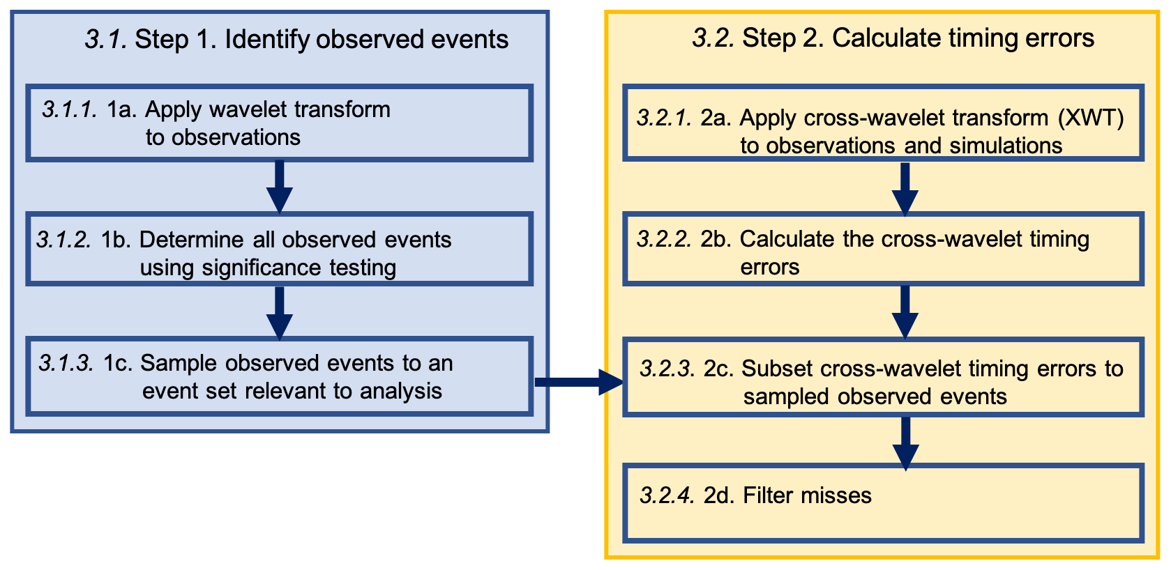
Figure 1 Flow chart of steps in the methodology. Although steps 1a–b and 2a–b can happen in parallel, step 2c needs to be preceded by step 1c.

NOAA's National Water Model (NWM; https://www.nco.ncep.noaa.gov/pmb/products/nwm/, last access: 8 May 2021) is an operational model that produces hydrologic analyses and forecasts over the continental United States (CONUS) and Hawaii (as of version 2.0). The model is forced by downscaled atmospheric states and fluxes from NOAA's operational weather models. Next, the Noah-MP (Noah-multiparameterization; Niu et al., 2011) land surface model calculates energy and water states and fluxes. Water fluxes propagate down the model chain through overland and subsurface (soil and aquifer representations) water routing schemes to reach a stream channel model. The NWM applies the three-parameter Muskingum–Cunge river routing scheme to a modified version of the National Hydrography Dataset Plus (NHDPlus) version 2 (McKay et al., 2012) river network representation (Gochis et al., 2020).

In this study, NWM simulations are taken from each version's retrospective runs (https://docs.opendata.aws/nwm-archive/readme.html, last access: 8 May 2021). These are continuous simulations (not cycles) run for the period from October 2010 to November 2016 and forced by the National Land Data Assimilation System (NLDAS)-2 product as atmospheric conditions. The nudging data assimilation was not applied in these runs. We use NWM discharge simulations from versions V1.0, V1.1, and V1.2 (not all versions may be publicly available).

The methodology developed in this paper is implemented in the R language and is made publicly available, as detailed in the code availability section at the end of the paper.

3 Methodology

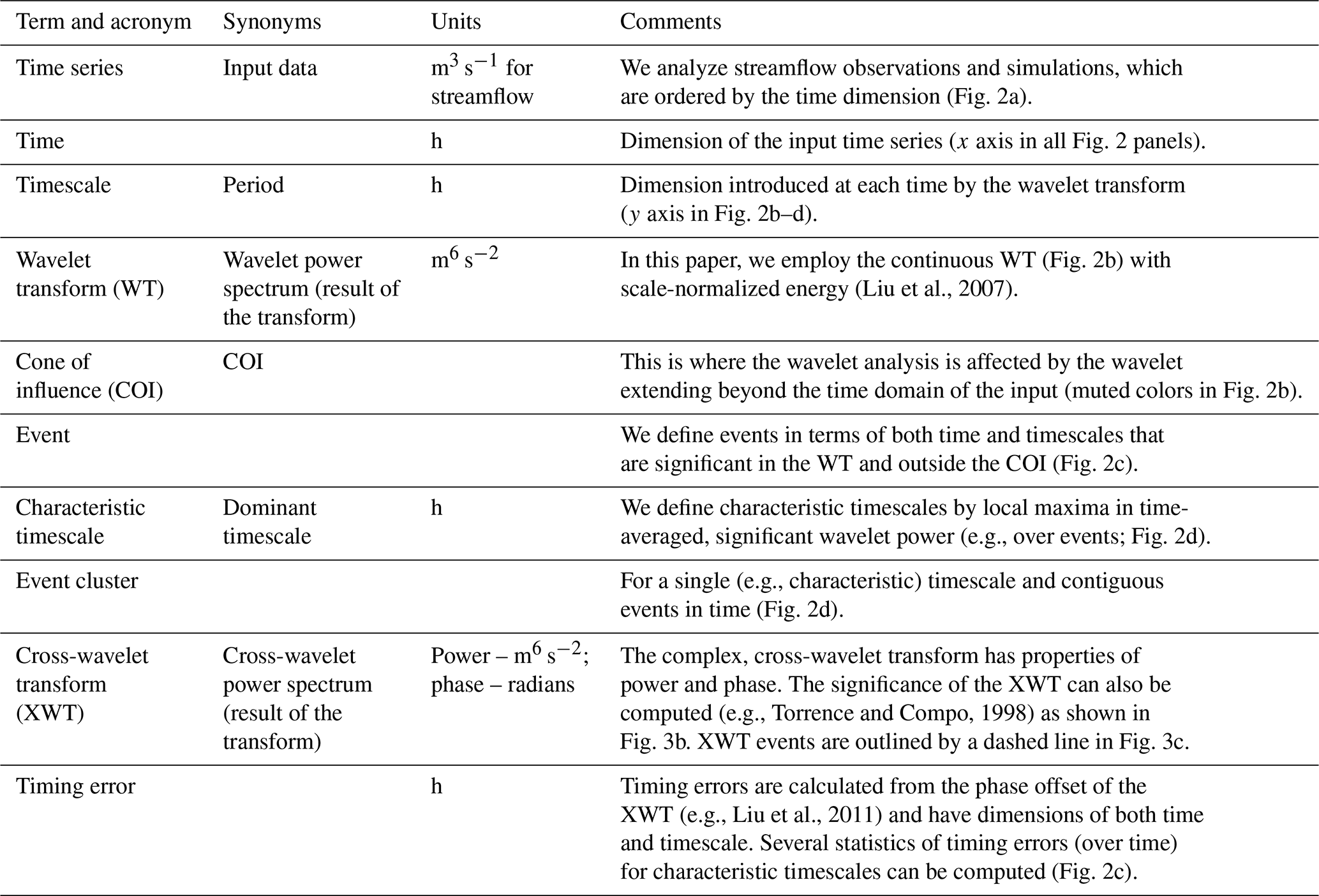
This section provides the description of the methodology using wavelets to identify events and estimate timing errors. The steps can be seen in the accompanying flowchart (Fig. 1) and nomenclature (Table 1), which define the key terms of the approach. To facilitate understanding, the steps are illustrated by an application of the methodology to an observed time series of an isolated peak in Onion Creek, TX, (Fig. 2a) and the synthetic modeled time series, which is identical to the observation time series but shifted 5 h in to the future (Fig. 3a; note the log scale).

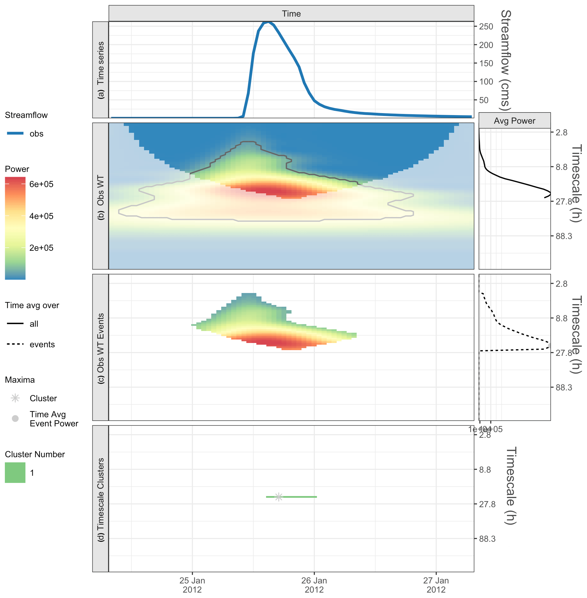
Figure 2 An isolated peak from Onion Creek, TX, showing the (a) observed time series, (b) observed wavelet power spectrum (left), and average power by timescale for all points (right). Panel (c)  shows the statistically significant wavelet power spectrum of events (left) and average power by timescale for all events, with maxima shown by gray dots (right). Panel (d) shows the characteristic scale event cluster (horizontal green line) and cluster maximum (asterisk).

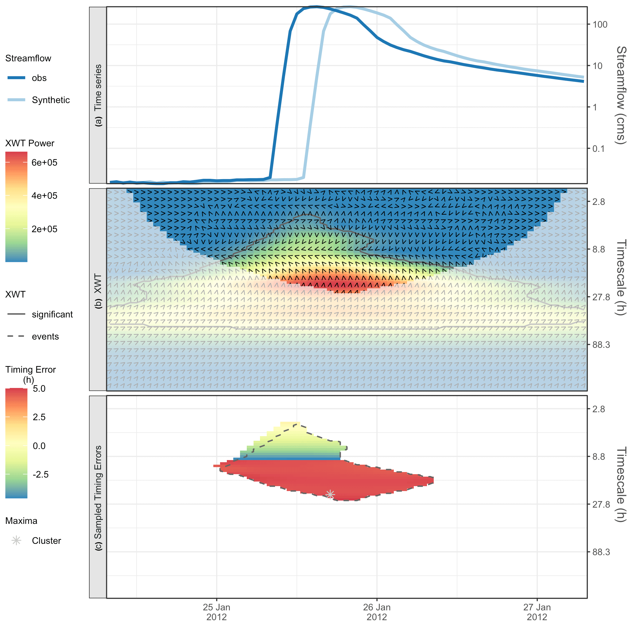
Figure 3 An isolated peak from Onion Creek, TX, and a synthetic + 5 h offset, showing the (a) observed and synthetic time series (note the logged y axis), (b) cross-wavelet (XWT) power spectrum, phase angles (arrows), and XWT significance (gray line). Panel (c)  shows the sampled timing errors for observed events (inside dashed contour indicates the intersection of XWT events with observed events), and the gray asterisk shows the cluster maximum from Fig. 2d.

Table 1 Nomenclature of terms used in the paper.

3.1 Step 1 – identify observed events

The first step is to identify a set of observed events for which the timing error should be calculated. We break this step into the following three substeps: 1a – apply the wavelet transform to observations; 1b – determine all observed events using significance testing; and 1c – sample observed events to an event set relevant to analysis.

3.1.1 Step 1a – apply wavelet transform to observations

First, we apply the continuous wavelet transform (WT) to the observed time series. The main steps and equations for the WT are provided here, though the reader is referred to Torrence and Compo (1998) and Liu et al. (2011) for more details.

Before applying the WT, a mother wavelet needs to be selected. In Torrence and Compo (1998), they discuss the key factors that should be considered when choosing the mother wavelet. There are four main considerations, including (i) orthogonal or nonorthogonal, (ii) complex or real, (iii) width, and (iv) shape. In this study, we follow Liu et al. (2011) in selecting the nonorthogonal and complex Morlet wavelet as follows:

$$\begin{array}{}\text{(1)}& \mathit{\psi }\left(n\right)={\mathit{\pi }}^{-\mathrm{1}/\mathrm{4}}{e}^{i{w}_{\mathrm{0}}n}{e}^{-n^{\mathrm{2}}/\mathrm{2}},\end{array}$$

where w₀ is the nondimensional frequency with a value of 6 (Torrence and Compo, 1998).

Once the mother wavelet is selected, the WT is applied to a time series, x_n, in which n goes from n=0 to $n=N-\mathrm{1}$ with a time step of δt. The WT is the convolution of the time series with the mother wavelet that has been scaled and normalized as follows:

$$\begin{array}{}\text{(2)}& W_n\left(s\right)=\sum _{n^{\prime }=\mathrm{0}}^{N-\mathrm{1}}{x}_{n^{\prime }}{\mathit{\psi }}^{*}\left[{\displaystyle \frac{(n^{\prime }-nt)\mathit{\delta }t}{s}}\right],\end{array}$$

where n^′ is the localized time in [0, N−1], s is the scale parameter, and the asterisk indicates the complex conjugate of the wavelet function. The wavelet power is defined as $\left|W_n^{\mathrm{2}}\right|$, which represents the squared amplitude of an imaginary number when a complex wavelet is used as in this study. We use the bias-corrected wavelet power (Liu et al., 2007; Veleda et al., 2012), which ensures that the power is comparable across timescales. We also identify a maximum timescale a priori that corresponds to our application. We select 256 h (∼10 d), but this number could be higher or lower for other applications, and there are no real penalties for using too high a maximum (lower than the annual cycle).

The wavelet transform (WT) expands the dimensionality of the original time series by introducing the timescale (or period) dimension. Wavelet power is also a function of both time and timescale (e.g., Torrence and Compo, 1998). This is illustrated in Fig. 2. The streamflow time series (Fig. 2a) is expanded into a 2-dimensional (2-D) wavelet power spectrum (Fig. 2b). Wavelet analysis can detect localized signals in the time series (Daubechies, 1990), including hydrologic time series, which are often irregular or aperiodic (i.e., events may be isolated and do not regularly repeat) or nonstationary. We note that, in many wavelet applications, timescale is referred to as “period”, and this axis is indeed the Fourier period in our plots. However, to emphasize that our study is more focused on irregular events and less on periodic behavior of time series, we use the term timescale to denote the Fourier period (and not wavelet scale).

Because we are applying the WT to a finite time series, there are timescale-dependent errors at the beginning and end times of the power spectrum, where the entirety of the wavelet at each scale is not fully contained within the time series. This region of the WT is referred to as the cone of influence or COI (Torrence and Compo, 1998). Figure 2b illustrates the COI as the regions in which the colors are muted; we ignore all results within the COI in this study.

We make several additional notes on the wavelet power and its representation in the figures. The units of the wavelet power are those of the time series variance (m⁶ s⁻² – meters to the sixth power per square second for streamflow), and it is natural to want to cast the power in a physical light or relate it to the time series variance. Indeed, the power is often normalized by the time series variance when presented graphically. However, it must be noted that the wavelet convolved with the time series frames the resulting power in terms of itself at a given scale. Wavelet power is a (normalized) measure of how well the wavelet and the time series match at a given time and scale. The power can only be compared to other values of power resulting from a similarly constructed WT. There are various transforms that can be applied to aid the graphical interpretation of the power (log and variance scaling), but the utility of these often depends on the nature of the individual time series analyzed. For simplicity, we plot the raw bias-rectified wavelet power in this paper.

3.1.2 Step 1b – determine all observed events using significant testing

In their seminal wavelet study, Torrence and Compo (1998) outline a method for objectively identifying statistical significance in the wavelet power by comparing the wavelet power spectra with a power spectra from a red noise process. Specifically, the observed time series is fitted with an order 1 autoregressive (AR1 or red noise) model, and the WT is applied to the AR1 time series. The power spectrum of the AR1 model provides the basis for the statistical significance testing. Significance is determined if the power spectra are statistically different using a chi-squared test.

Figure 2b shows significant (>=95 % confidence level) regions of wavelet power inside black contours. Statistical significance indicates wavelet power that falls outside the time series background statistical power based on an AR1 model of the time series. Statistical significance of the wavelet power can be thought of as events in the wavelet domain. We define events as regions of significant wavelet power outside the COI. Figure 2c displays the wavelet power for the events in this time series. We emphasize that events defined in this way are a function of both time and timescale and that, at a given time, events of different timescales can occur simultaneously.

3.1.3 Step 1c – sample observed events to an event set relevant to analysis

Step 1b results in the identification of all events at all timescales and times. In this substep, the event space is sampled to suit the particular evaluation. Torrence and Compo (1998) offer the following two methods for smoothing the wavelet plot that can increase significance and confidence: (i) averaging in time (over timescale) or (ii) averaging in timescale (over time). Because the goal of this paper is to evaluate model timing errors over long simulation periods, we choose to sample the event space based on averaging in timescale. Although for some locations there may be physical reasons to expect certain timescales to be important (e.g., the seasonal cycle of snowmelt), the most important timescales at which hydrologic signals occur at a particular location are not necessarily known a priori. Averaging events in timescale can provide a useful diagnostic by identifying the dominant, or characteristic, timescales for a given time series. Averaging many events in a timescale can filter noise and help reveal the expected timescales of dominant variability corresponding to different processes or sets of processes.

In our analysis, we seek to uncover the dominant event timescales and to evaluate modeled timing errors on them. The following points articulate our methodological choices for summarizing the observed events:

• Calculate the average event power in each timescale. Considering only the statistically significant areas of the observed wavelet spectrum, calculate the average power in each timescale (Fig. 2c, right panel). We point out that calculating the average power over events is different to what is found by averaging across all time points, which does not take statistical significance into consideration (Fig. 2b, right panel).

• Identify timescales of absolute and local maxima in time-averaged power. After obtaining the average event power as a function timescale (Fig. 2c, right panel), the local and absolute maximums for average event power can be determined. In the Onion Creek case, there is a single maximum at 22 h (gray dot in Fig. 2c, right panel). The timescales corresponding to the absolute and local maxima of the average power of the observed time series are called the characteristic timescales used for evaluation. This is the first subset of the events, i.e., all events that fall within the characteristic timescales. For a single characteristic timescale, contiguous events in time are called event clusters (horizontal line in Fig. 2d).

• Identify events with maximum power in each event cluster. For all timescales, we identify the event with maximum power in each event cluster. This is the second event subset, i.e., all events with maximum power in each cluster that fall within a characteristic timescale (asterisk in Fig. 2d); these are called cluster maxima.

3.2 Step 2 – calculate timing errors

Step 1 identifies observed events by applying a wavelet transform to the observed time series. To calculate the timing error of a modeled time series, we perform its cross-wavelet transform with the observed time series. Figure 3a shows the observed and modeled time series used in our illustration of the methodology, i.e., the observed is the same isolated peak from Onion Creek, TX, as in Fig. 2a, and the synthetic modeled time series adds a prescribed timing error of +5 h to the observed. (Note that while the observed time series is identical in both, Figs. 2a and 3a have linear and log ₁₀ axes, respectively.)

3.2.1 Step 2a – apply cross-wavelet transform (XWT) to observations and simulations

The cross-wavelet transform (XWT) is performed between the observed and synthetic time series. Given the WTs of an observed time series $W_n^X\left(s\right)$ and a modeled time series $W_n^Y\left(s\right)$, the cross-wavelet spectrum can be defined as follows:

$$\begin{array}{}\text{(3)}& W_n^{XY}\left(s\right)=W_n^X\left(s\right)W_n^{Y^{*}}\left(s\right),\end{array}$$

where the asterisk denotes the complex conjugate. The cross-wavelet power is defined as $\left|W_n^{XY}\right(s\left)\right|$ and signifies the joint power of the two time series. The XWT between the Onion Creek observations and the synthetic 5 h offset time series is shown in Fig. 3b, with power represented by the color scale.

Similar to step 1b of the WT, we can also calculate areas of significance for the XWT power as shown by the black contour in Fig. 3b. For the XWT, significance is calculated with respect to the theoretical background wavelet spectra of each time series (Torrence and Compo, 1998). We define XWT events as points of significant XWT power outside the COI. XWT events indicate significant joint variability between the observed and modeled time series. Below, in step 2d, we employ XWT events as a basis for identifying hits and misses on observed events for which the timing errors are calculated. Figure 3c shows the observed events (colors) and the intersection between the observed and XWT events (dashed contour). As described later, this intersection (inside dashed contour) is a region of hits where timing errors are considered valid. Note that the early part of the observed events at shorter timescales is not in the XWT events. This is because the timing offset in the modeled time series misses the early part of the observed event for some timescales.

3.2.2 Step 2b: calculate the cross-wavelet timing errors

For complex wavelets, such as the Morlet used in this paper, the individual WTs include an imaginary component of the convolution. Together, the real and imaginary parts of the convolution describe the phase of each time series with respect to the wavelet. The cross-wavelet transform combines the WTs in conjugate, allowing the calculation of a phase difference or angle (radians), which can be computed as follows:

$$\begin{array}{}\text{(4)}& {\mathit{\varphi }}_n^{XY}\left(s\right)={\tan }^{-\mathrm{1}}\left[{\displaystyle \frac{I\left(\mathcal{I}\langle s^{-\mathrm{1}}{W}_n^{XY}\left(s\right)\rangle \right)}{\mathcal{R}\left(\mathcal{I}\langle s^{-\mathrm{1}}{W}_n^{XY}\left(s\right)\rangle \right)}}\right],\end{array}$$

where ℐ is the imaginary and ℛ is the real component of $W_n^{XY}\left(s\right)$. The arrows in Fig. 3b indicate the phase difference for our example case, which is used to calculate the timing errors. Note that these are calculated at all points in the wavelet domain.

The distance around the phase circle at each timescale is the Fourier period (hours). We convert the phase angle into the timing errors (hours) as in Liu et al. (2011) as follows:

$$\begin{array}{}\text{(5)}& \mathrm{\Delta }{t}_n^{XY}\left(s\right)={\mathit{\varphi }}_n^{XY}\left(s\right)\cdot T/\mathrm{2}\mathit{\pi },\end{array}$$

where T is the equivalent Fourier period of the wavelet. Note that the maximum timing error which can be represented at each timescale is half the Fourier period because the phase angle is in the interval (−π, π). In other words, only timescales greater than 2E can accurately represent a timing error E. Because the range of the arctan function is limited by ±π, true phase angles outside this range alias to angles inside this range. (For example, the phase angles 1.05⋅π and $-\mathrm{0.95}\cdot \mathit{\pi }$ are both assigned to $-\mathrm{0.95}\cdot \mathit{\pi }$). Also note that, when the wavelet transforms are approximately antiphase, the computed phase differences and timing errors produce corresponding bimodal distributions given the noise in the data. Figure 3c shows phase aliasing in the negative timing errors at timescales less than 10 h, which is double the 5 h synthetic timing error we introduced. The bimodality of the phase and timing are also seen at the 10 h timescale when the timing errors abruptly change sign (or phase by 2π). We note the convention used is that the XWT produces timing errors that are interpreted as modeled minus observed, i.e., positive values mean the model occurs after the observed. Positive 5 h timing errors in Fig. 3c describe that the model is late compared to the observations as seen in the hydrographs in the top panel (Fig. 3a).

3.2.3 Step 2c – subset cross-wavelet timing errors to sampled observed events

Step 2b results in an estimate of timing errors for all times and timescales in the cross-wavelet transform space. In our application, we are interested in the timing errors that correspond to the identified sample of observed events, especially for the maximum power events in each cluster for each characteristic timescale. In the synthetic Onion Creek example, the point of interest in the wavelet transform of the observed time series, used to sample the timing errors produced by the XWT, is shown by the gray asterisk in Fig. 3c.

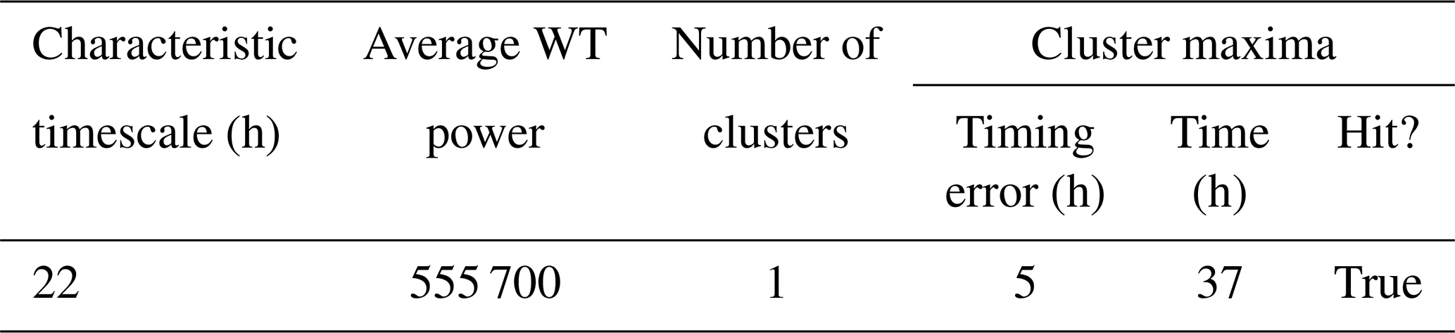
The results for the synthetic Onion Creek example are summarized in Table 2. For the identified characteristic timescale of 22 h in the observed wavelet power (which had an average WT power of 555 700 m⁶ s⁻²; see Fig. 2c on the right), there was one event cluster, and the timing error at the cluster maximum was 5 h, and it occurred at hour 37 of the time series.

Table 2 Summary of timing error results for cluster maxima for the isolated peak and prescribed 5 h offset from Onion Creek, TX.

3.2.4 Step 2d – filter misses

The premise of computing a timing error between the observed and modeled time series is that they share common events which can be meaningfully compared. In a two-way contingency analysis of events, a hit refers to when the modeled time series reproduces an observed event. When the modeled time series fails to reproduce an observed event, it is termed a miss. In the case of a miss, it does not make sense to include the timing error in the overall assessment. Once the characteristic timescales of the observed event spectrum are identified and event cluster maxima are located, timing errors are obtained at these locations in the XWT. In this step, the significance of the XWT on these event cluster maxima is used to decide if the model produced a hit or a miss for each point and to determine if the timing error is valid. As previewed above, Fig. 3c shows the observed events (colors), and the dashed contour shows the intersection between the observed and XWT events. Regions of intersection between observed events and XWT events are considered model hits, and observed events falling outside the XWT events are considered misses. Because we constrain our analysis to observed events in the wavelet power spectrum, we do not consider either of the remaining categories in a two-way analysis (false alarms and correct negatives). We note that a complete two-way event analysis could, alternatively, be constructed in the wavelet domain based on the Venn diagram of the observed and modeled events without necessarily using the XWT. We choose to use the XWT events because the XWT is the basis of the timing errors.

In the synthetic example of Onion Creek, a single characteristic timescale and event cluster yields a single cluster maximum, as shown by the asterisk in Fig. 3c. Because this asterisk falls both within the observed and XWT events, it is a hit, and the timing error at that point is valid (Table 2). For a longer time series, as seen in subsequent examples, a useful diagnostic and complement to the timing error statistics at each characteristic timescale is the percent hits. When summarizing timing error statistics for a timescale, we drop misses from the calculation and the percent hits indicates what portion of the time series was dropped (percent misses is equal to 100 − percent hits). In our tables, we provided timing error statistics for hits only.

4 Results

In the previous section, we illustrate the method using an isolated peak and a prescribed timing error. In this section, we demonstrate the method using NWM model simulations which introduce greater complexity and longer time series. Finally, we show version-over-version comparisons for 5-year simulations to illustrate the utility for evaluation.

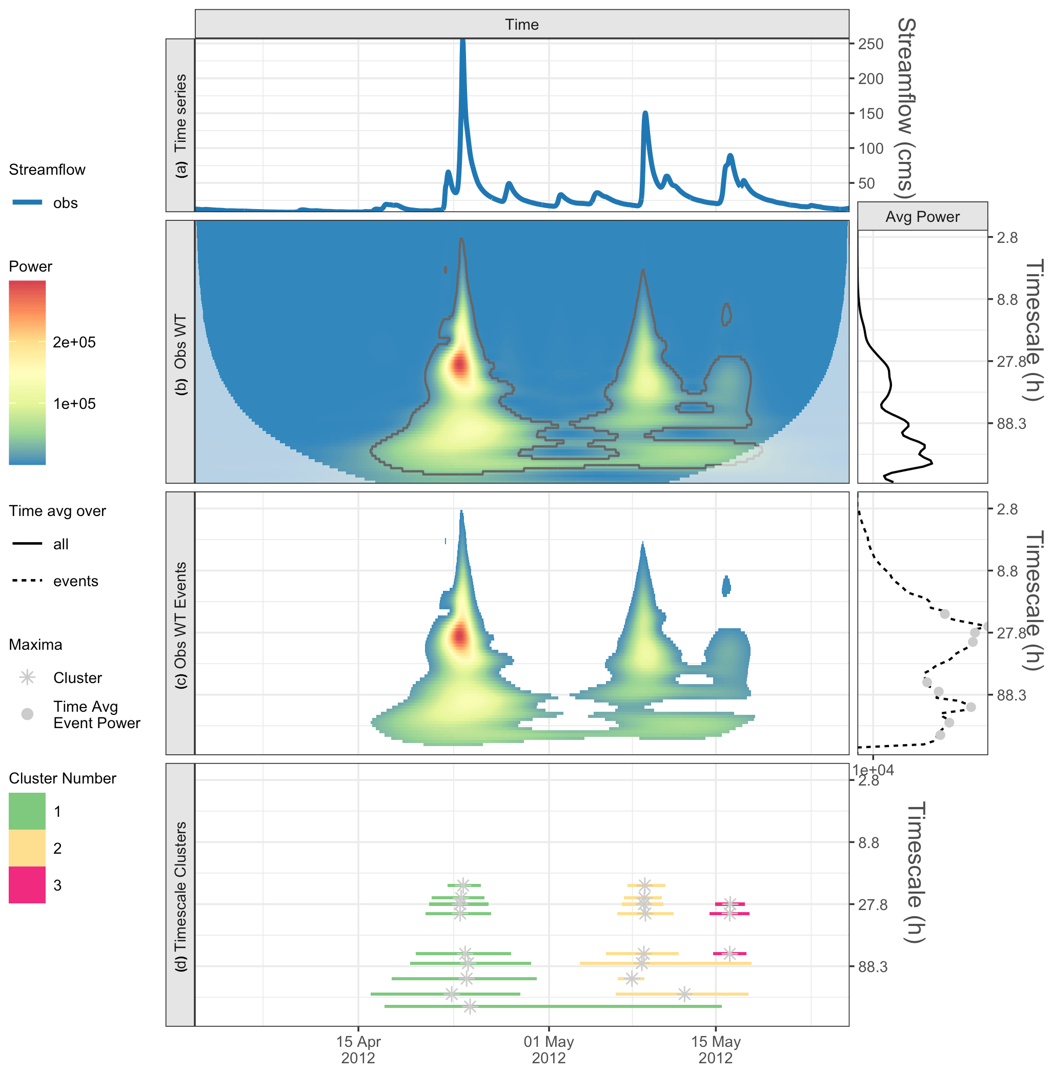
Figure 4 For the 3-month time series from the Pemigewasset River, NH, panel (a) shows the observed time series, and (b) shows the observed wavelet power spectrum (left) and average power by timescale for all points (right). Panel (c) shows the statistically significant wavelet power spectrum of events (left) and average power by timescale for all events, with maxima shown by gray dots (right). Panel (d) shows the characteristic scale event clusters (horizontal lines) and cluster maxima (gray asterisks).

4.1 Demonstration using NWM data

4.1.1 Pemigewasset River, NH

This example uses a 3-month time series from the Pemigewasset River, NH, to examine multiple peaks in the hydrograph (Fig. 4a). It is fairly straightforward to pick out three main peaks with the naked eye. From step 1 of our method, the wavelet transform is applied to the observations (Fig. 4b, left panel; Fig. 4c, left panel), revealing up to three event clusters, depending on the characteristic timescale examined (Fig. 4d). When we plot the average event power by timescale (Fig. 4c, right panel), we see that there are nine relative maxima (small gray dots); hence, there are nine characteristic scales for this example. The cluster maxima (gray asterisks) for each observed event cluster are shown in Fig. 4d.

Figure 5 For 3-month time series from Pemigewasset River, NH, panel (a) shows the observed and simulated NWM time series (note the logged y axis), (b)  shows the cross-wavelet (XWT) power spectrum (colors), phase angles (arrows), and statistically significant XWT events (solid contours), and (c) shows the sampled timing errors for observed events (inside dashed contour indicates intersection of XWT events with observed events) and cluster maxima (gray asterisks).

Next, we compare the observed time series with the simulation from the NWM V1.2 (Fig. 5a) and follow step 2 of our method: (a) apply the cross-wavelet transform (Fig. 5b colors), (b) calculate the timing error for all observed events from the phase difference (Fig. 5b arrows), (c) subset the timing errors to the observed cluster maxima (Fig. 5c asterisks), and (d) retain only modeled hits (Fig. 5c asterisks within the dashed contours). Table 3 is ordered, by characteristic timescales, from highest to lowest average power; we only show the top five characteristic scales. The absolute maximum of the time average event spectrum has a timescale equal to 24.8 h; for cluster one, the model is nearly 11 h late, and cluster two is early (−3.5 h). Both are hits, and the average timing error is 3.5 h late. However, for the next timescale (=27.8 h), the third cluster maximum is a miss, so its timing error is reported as n/a (not applicable) and is not included in the average. This miss can be seen in Fig. 5c where the cluster 3 asterisk falls just outside the XWT events for the 27.8 h, timescale. Moreover, this miss can also be interpreted from the comparison of the hydrographs in Fig. 5a where the modeled third peak does not reasonably approximate the magnitude of the observed peak. Interestingly, while it is a narrow miss at the shorter timescale of 27.8 h, the associated (third) cluster maxima at the next most powerful characteristic timescale (33.1 h) is a hit. This reflects that the hydrograph is insufficiently peaked for this event but does have some of the observed, lower-frequency variability. Overall, the characteristic timescale of 33.1 h has timing results similar to the 27.8 h timescale, with the exception of the third cluster maximum. This raises the question of whether these are distinct characteristic timescales. In Sect. 5, we discuss smoothing the time average event power by timescale to address this issue.

The characteristic timescale with the fourth-highest time-averaged power occurs at 111 h, which is a different order of magnitude, suggesting that this may have a different physical process driving it. At this timescale, the model is late in both event clusters (10 and 16 h). Results are similar for the next timescale of 148 h. We do not show results for the remaining four characteristic timescales with lower average power, since they have similar characteristic timescale values and associated timing errors to what has already been shown.

Figure 6 For a 1-year time series from Taylor River, CO, panel (a) shows the observed time series, and (b) shows observed wavelet power spectrum (left) and average power by timescale for all points (right). Panel (c) shows the statistically significant wavelet power spectrum of events (left) and average power by timescale for all events, with maxima shown by gray dots (right). Panel (d) shows the characteristic scale event clusters (horizontal lines).

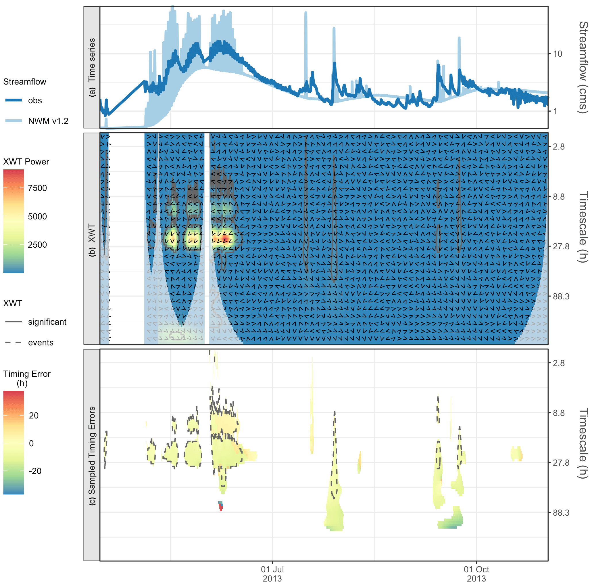
Figure 7 For a 1-year time series from Taylor River, CO, panel (a) shows the observed and simulated NWM time series (note the logged y axis), (b) shows the cross-wavelet (XWT) power spectrum (colors), phase angles (arrows), and statistically significant XWT events (solid contours). Panel (c) shows the sampled timing errors for observed events (inside dashed contour indicates intersection of XWT events with observed events).

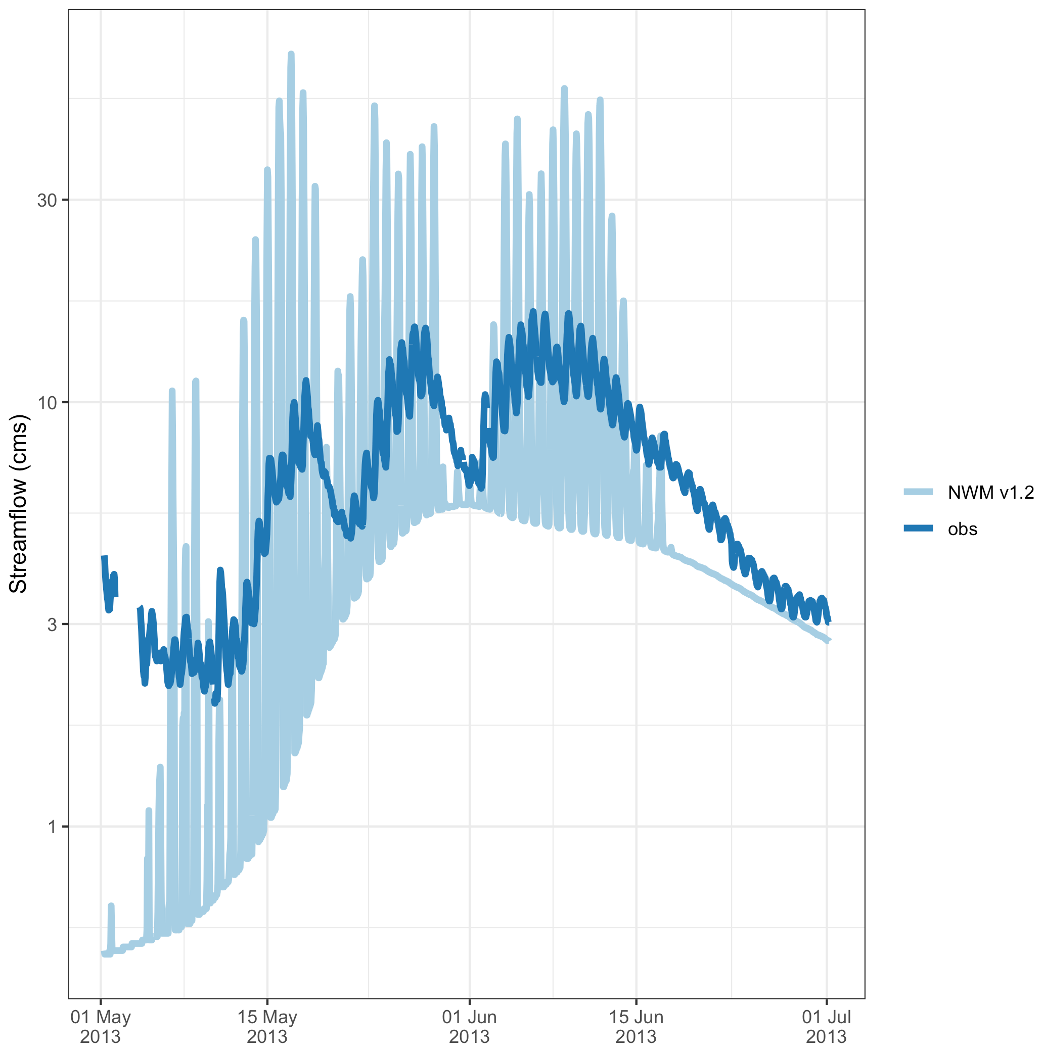
Figure 8 Magnified view of the spring runoff of a 1-year time series for Taylor Park, CO, showing the observed and simulated NWM time series.

4.1.2 Taylor River, CO

In this example, we examine a 1-year time series from Taylor River, CO, that illustrates hydrograph peaks driven by different processes. The Taylor River is in a mountainous area where the spring hydrology is dominated by snowmelt runoff. Figure 6a shows the time series from Taylor River, CO, where we can see the snowmelt runoff in spring and also several peaks in summer, likely driven by summer rains. Figure 6b shows the WT and illustrates how missing data is handled. This results in additional COIs (muted colors) to account for the edge effects, and areas of the COI are ignored in our analyses.

From the statistically significant events in the WT, we see the peak in the characteristic timescales at 23.4 h (Fig. 6c, right), and there is another maxima at the 99 and 118 h timescales. The process-based shift in dominant timescales is evident in the wavelet power (Fig. 6b and c). The 23.4 h timescale is dominant before 1 July, during snowmelt runoff, and then shifts to the 99 and 118 h timescales, relating to flows from summer rains. In step 2, we compare the observed time series with the simulation from the NWM V1.2 (Fig. 7a); here, it is useful to magnify the spring melt season time series (Fig. 8), where we see that the amplitude of the diurnal signal is too high, but it is hard to visually tell much about the timing error. Next, the cross-wavelet transform (Fig. 7b) and timing errors are calculated (Fig. 7c). The results are summarized in Table 4. Starting with the dominant 23.4 h timescale, we see that there are 11 clusters, that 73 % ($=\mathrm{8}/\mathrm{11}$ cluster maxima) are hits, and that the model is generally early (the mean is 6 h early). For the 118 and 99 h timescales, there are no hits. This suggests that we are confident in the timing errors of the model for the diurnal snowmelt cycle, and these timing errors can be used as guidance for model performance and model improvements. However, the model does not successfully reproduce key variability during the summer, and timing errors are not valid at this timescale. This underscores the key point that timing errors are timescale dependent and can help diagnose which processes to target for improvements.

Table 3 For a 3-month time series from Pemigewasset River, NH, by characteristic timescale, this is a summary of the timing error results for cluster maxima that were hits when using NWM v1.2.

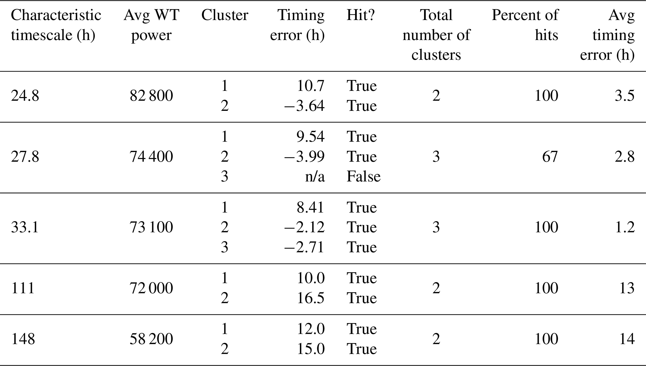
The term n/a stands for not applicable.

Table 4 For a 1-year time series from Taylor River, CO, by characteristic timescale, this is a summary of the timing error results for the cluster maxima that were hits when using NWM v1.2.

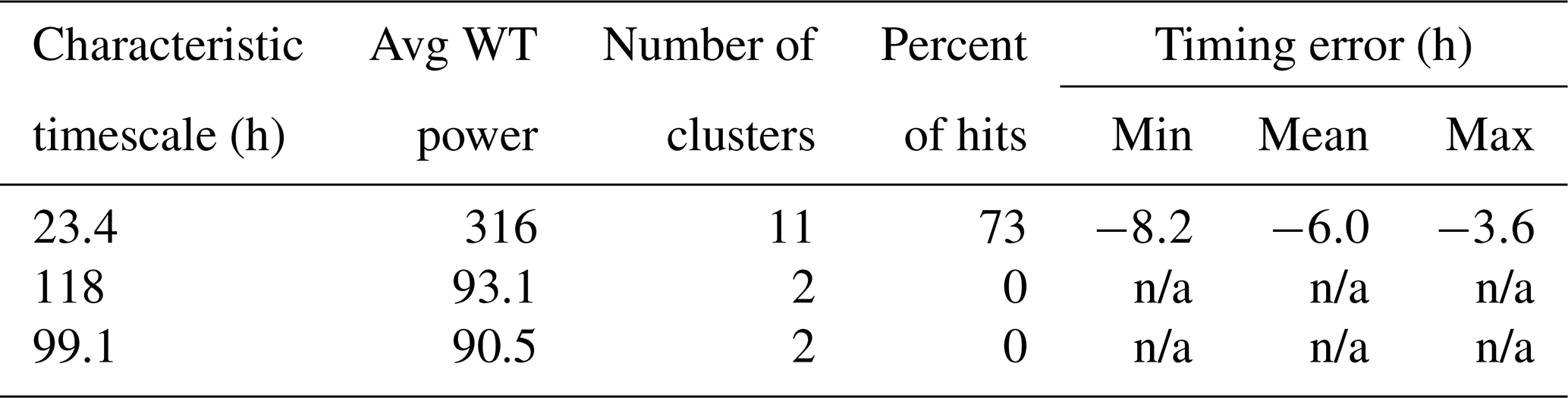
The term n/a stands for not applicable.

4.2 Evaluating model performance

Finally, we show how the methodology can be used for evaluating performance changes across NWM versions. We point out that none of the NWM version upgrades were targeting timing errors, so these results just provide a demonstration. We use 5-year observed and modeled time series at the three locations, namely Onion Creek, TX, Pemigewasset River, NH, and Taylor River, CO.

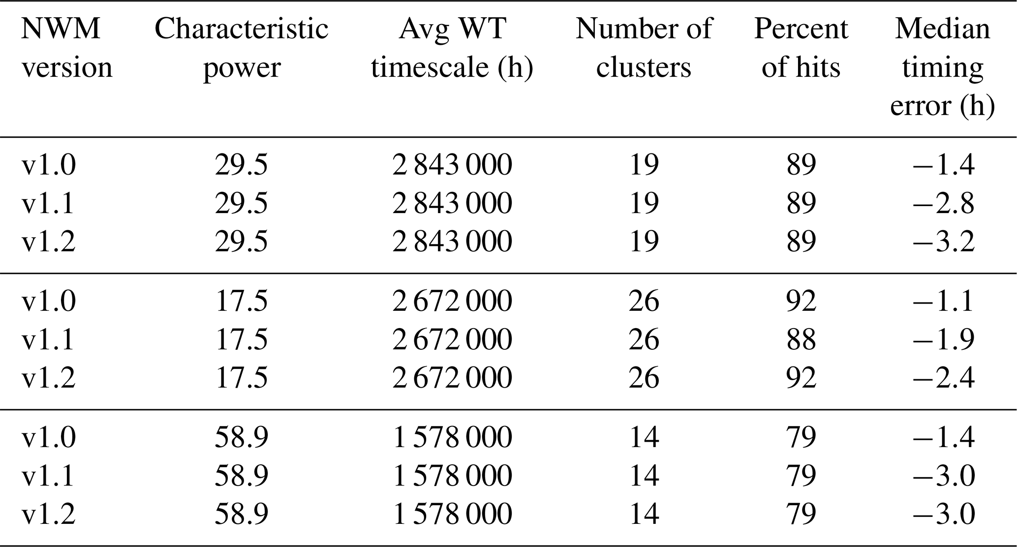
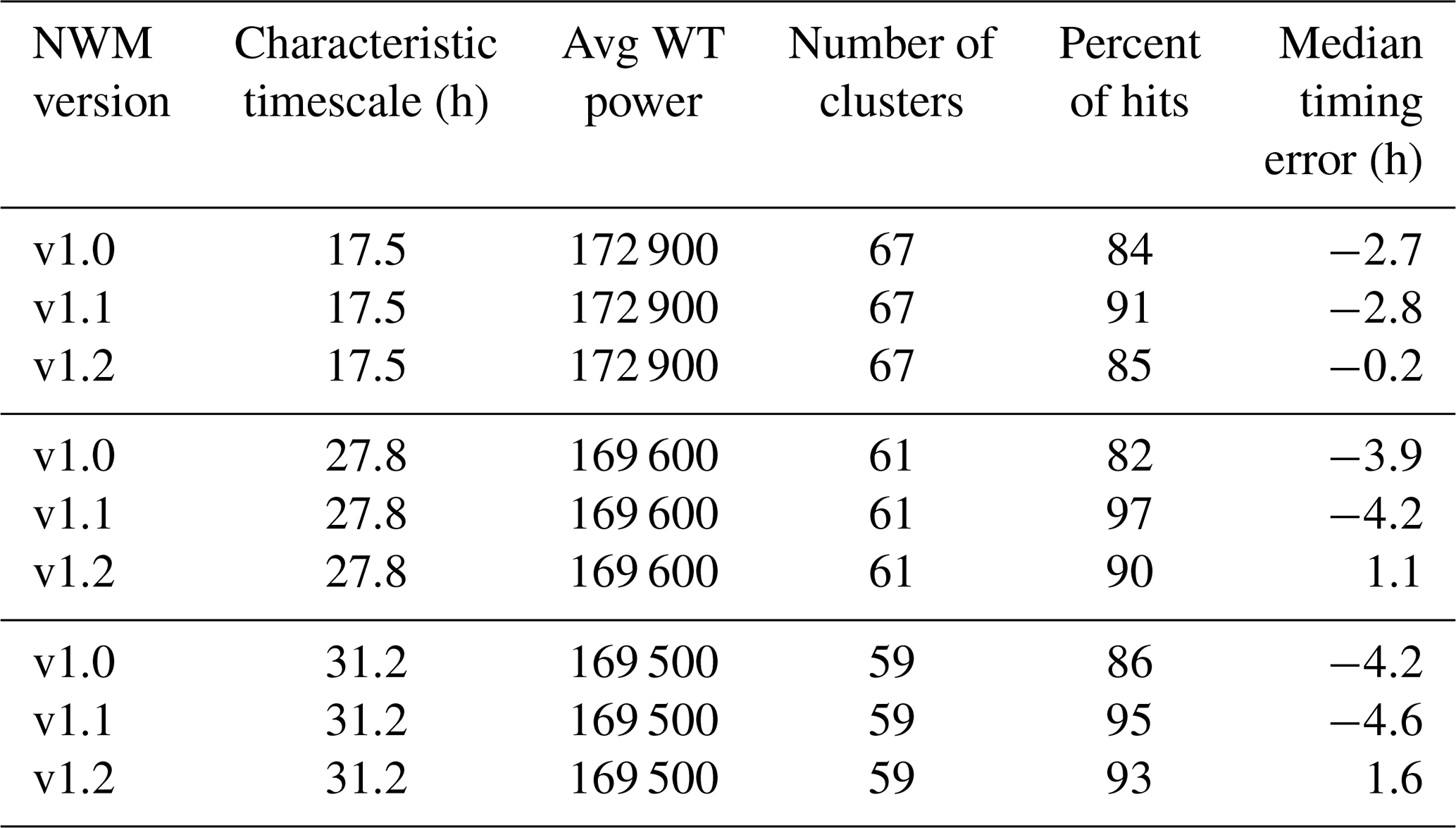
For Onion Creek, Table 5 summarizes the results for the three most important timescales, and Fig. 9 provides a graphical representation of these timing errors (hits only). For the dominant 29.5 h timescale and for all model versions, there were 19 cluster maxima, 89.5 % of which were hits, with a median timing error of 1.4 h early. However, the model shows progressively earlier timing errors with increasing version (Fig. 9). The results are similar for the other two characteristic timescales.

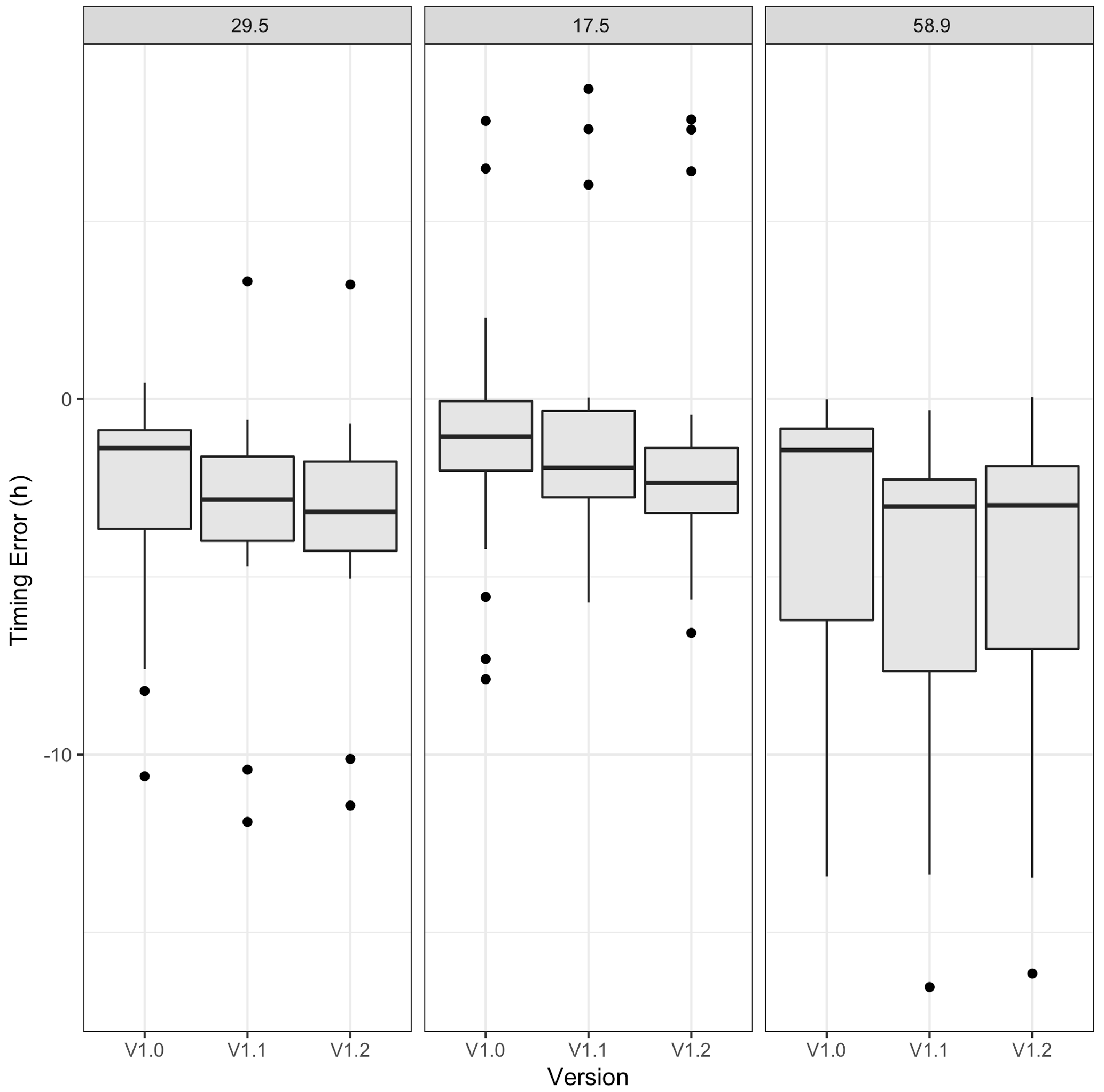
Figure 9 A 5-year time series from Onion Creek, TX, which compares cluster maxima timing error distributions for the top three characteristic timescales (see panel title) across NWM versions.

Table 5 Summary of timing errors from cluster maxima that were hits for 5-year time series from Onion Creek, TX.

For Pemigewasset River, Table 6 summarizes the results for the three most important timescales, and Fig. 10 provides a graphical representation of the timing errors (hits only). At this location, the median timing error improved with NWM V1.2, moving closer to zero. While the distribution of the timing errors became less biased than the previous versions, it also became wider (Fig. 10). Over the time series, there were between 59 and 76 event clusters. Interestingly, the hit rate for all timescales was best for NWM V1.1, though its timing errors are broadly the worst. From NWM V1.0 to NWM V1.2, improvements to both hit rate and median timing errors were obtained at all timescales.

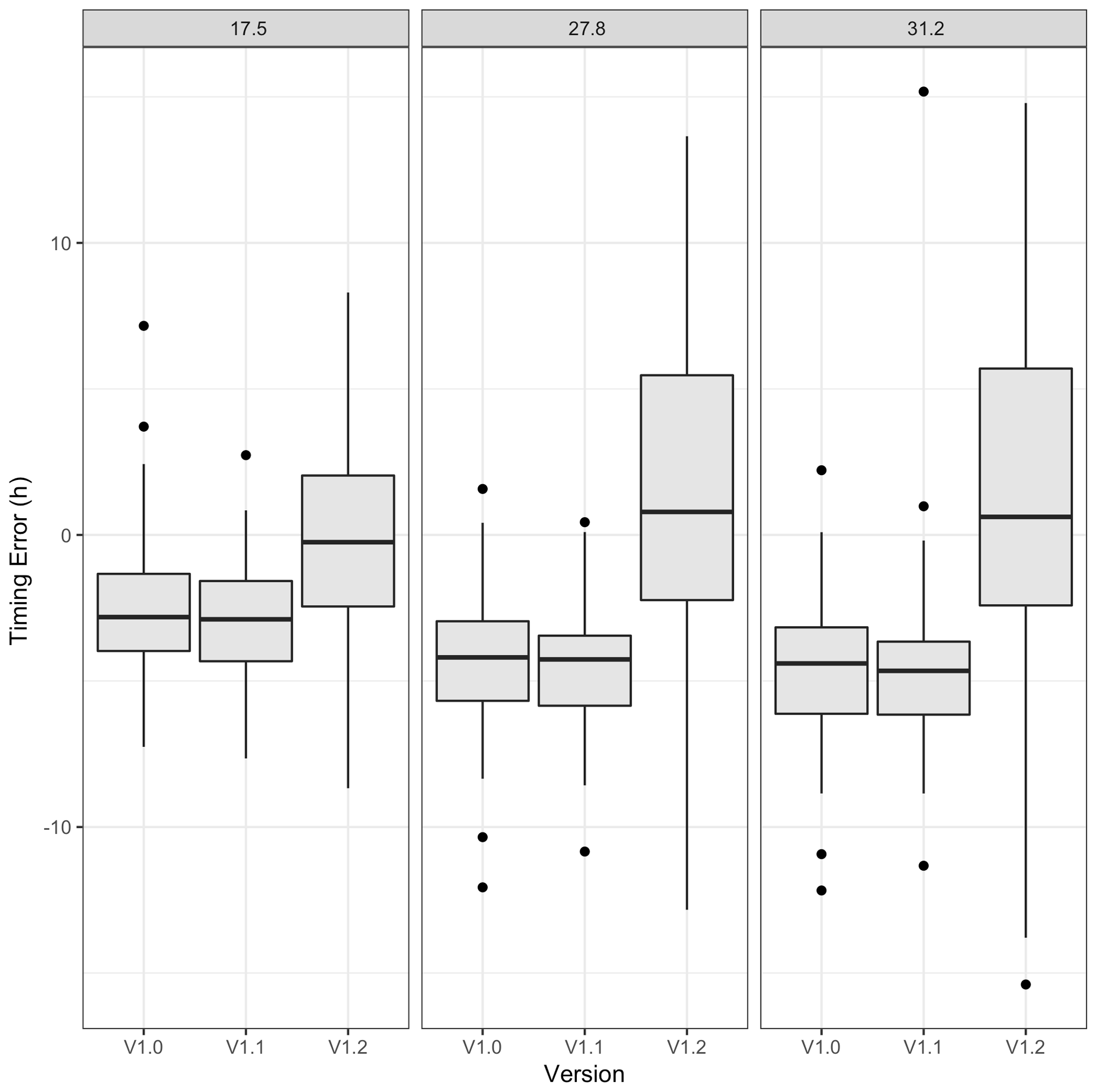
Figure 10 A 5-year time series from Pemigewasset River, NH, which compares cluster maxima timing error distributions for the top three characteristic timescales (see panel title) across NWM versions.

Table 6 Summary of timing errors from cluster maxima that were hits for 5-year time series from Pemigewasset River, NH.

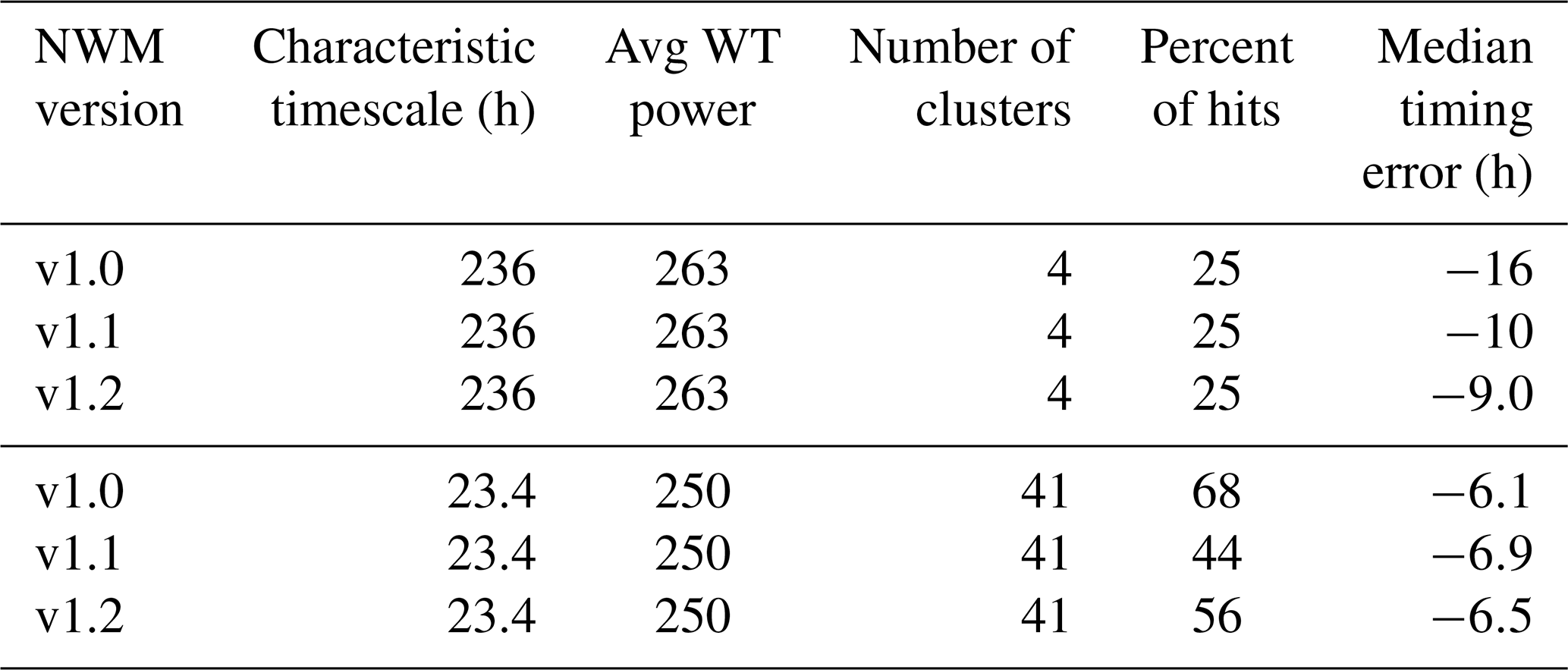
For Taylor River, Table 7 summarizes the results for the two most important timescales. For the characteristic timescale of 235 h (∼10 d), there are only four event clusters, and each model version has only one hit. The timing of this hit improves by roughly half its error from NWM V1.0 to NWM V1.2 in going from 16 to 9 h. The 23.4 h timescale has 41 event clusters, with a hit rate varying considerably by version. The median timing error is fairly consistent with version, however, ranging from 6 to 7 h early.

Table 7 Summary of timing errors from cluster maxima that were hits for 5-year time series of Taylor River, CO.

5 Discussion and conclusions

In this paper, we develop a systematic, data-driven methodology to objectively identify time series (hydrograph) events and estimate timing errors in large-sample, high-resolution hydrologic models. The method was developed towards several intended uses. First, it was primarily developed for model evaluation, so that model performance can be documented in terms of defined standards. We illustrate this with the version-over-version NWM comparisons. Second, it can be used for model development, whereby potential timing error sources can be diagnosed (by timescale) and targeted for improvement. Related to this point, and given the advantages of calibrating using multiple criteria (e.g., Gupta et al., 1998), timing errors could be used as part of a larger calibration strategy. However, minimizing timing errors at one timescale may not translate to improvements in timing errors (or other metrics) at other timescales. Wavelet analysis has also been used directly as an objective function for calibration, although a difficulty arises in determining which similarity measure to use (e.g., Schaefli and Zehe, 2009; Rathinasamy et al., 2014). Future research will investigate the application of the timing errors presented here for calibration purposes. Finally, the approach can be used for model interpretation and forecast guidance, as estimating timing errors provides characterization of the timing uncertainty (i.e., for a given timescale, the model is generally late or early) or confidence.

Given the fact that several subjective choices were made specific to our application and goals, it is important to highlight that we have made the analysis framework openly available (detailed in the code availability section below), so the method can be adapted, extended, or refined by the community right away. We look at timing errors from an observed event set relevant to our analysis, but there are other ways to subset the events that might be more suitable to other applications. For example, we focus on the event cluster maxima, but one could also examine the event cluster means or the local maxima along time. Another alternative to finding the event cluster maxima (i.e., for a given timescale) would be to identify the event with maximum power in islands of significance across timescales, i.e., contiguous regions of contiguous significance across both time and timescale. This approach would ignore that multiple frequencies can be important at once. Moreover, defining such islands is not straightforward. A different approach could be desirable if one suspected nonstationarity in the characteristic timescales over the time series. Then perhaps a moving average in timescale could be employed to identify characteristic timescales. In our approach, we define the event set broadly. However, it could be subset using streamflow thresholds (e.g., for flooding events) to compare events in the wavelet domain with traditional peak-over-threshold events. For example, Fig. 11 shows the maximum streamflows for the event set from the 5 year time series at Taylor River. This figure shows that all events identified by the algorithm are not necessarily high-flow events (i.e., the maximum streamflow peaks are lower for the 23.4 h timescale compared to the 235.6 h timescale). To compare with traditional peak-over-threshold approaches, this event set could be filtered to include only events above a given threshold (i.e., events in both the wavelet and time domains).

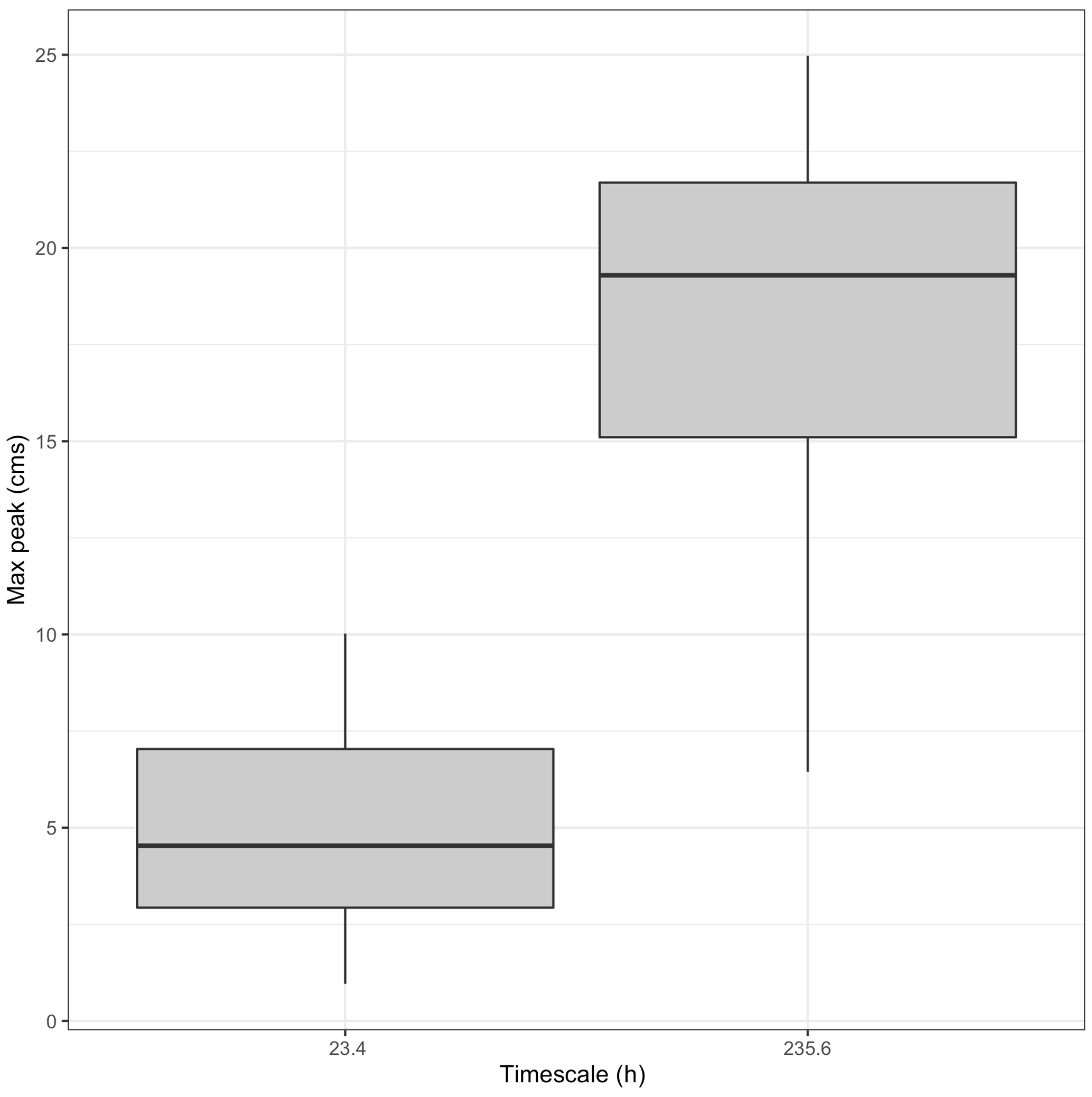
Figure 11 A 5-year time series from Taylor River, CO, showing the top two characteristic timescales and maximum streamflow peak distributions for each event (using cluster maxima) in cubic meters per second (m³ s⁻¹).

Another point that arises is how many characteristic timescales should be examined and the similarity of adjacent characteristic timescales. In our method, we average the power in timescales and identify characteristic scales at every absolute and relative maxima. As seen in the illustrative examples, this can result in multiple characteristic scales, some of which can be quite similar, suggesting that events at those scales are from similar or related processes. A solution could be to smooth the average power by timescale, which would reduce the number of local maxima, or to look at timing errors within a band of timescales. It is also important to note that the characteristic scales are data driven, so they will change with different lengths of observed time series. Longer runs capture more events and should converge on the more dominant timescales and events for a location. However, for performance evaluation, overlapping time periods for observed and modeled time series are needed.

In our application of the WT, we follow Liu et al. (2011) and select the Morlet as the mother wavelet. However, results are sensitive to the mother wavelet selected. Further discussion of mother wavelet choices can be found in Torrence and Compo (1998) and in ElSaadani and Krajewski (2017).

In summary, this paper provides a systematic, flexible, and computationally efficient methodology for calculating model timing errors that is appropriate for model evaluation and comparison and is useful for model development and guidance. Based on the wavelet transform, the method introduces timescale as a property of timing errors. The approach also identifies streamflow events in the observed and modeled time series and only evaluates timing errors for modeled events which are hits in a two-way contingency analysis. Future work will apply the approach to identify characteristic timescales across the United States and to assess the associated timing errors in the NWM.