Event and seasonal hydrologic connectivity patterns in an agricultural headwater catchment

Connectivity of the hillslope and the stream is a non-stationary and non-linear phenomenon dependent on many controls. The objective of this study is to identify these controls by examining the spatial and temporal patterns of the similarity between shallow groundwater and soil moisture dynamics and streamflow dynamics in the Hydrological Open Air Laboratory (HOAL), a small (66 ha) agricultural headwater catchment in Lower Austria. We investigate the responses to 53 precipitation events and the seasonal dynamics of streamflow, groundwater and soil moisture over 2 years. The similarity, in terms of Spearman correlation coefficient, hysteresis index and peak-to-peak time, of groundwater to streamflow shows a clear spatial organization, which is best correlated with topographic position index, topographic wetness index and depth to the groundwater table. The similarity is greatest in the riparian zone and diminishes further away from the stream where the groundwater table is deeper. Soil moisture dynamics show high similarity to streamflow but no clear spatial pattern. This is reflected in a low correlation of the similarity with site characteristics. However, the similarity increases with increasing catchment wetness and rainfall duration. Groundwater connectivity to the stream on the seasonal scale is higher than that on the event scale, indicating that groundwater contributes more to the baseflow than to event runoff.

1 Introduction

Hydrologic connectivity is an important control on runoff generation in response to precipitation events (van Meerveld et al., 2015; Penna et al., 2015; Zuecco et al., 2016). It is usually defined as the ability of water, solutes or microorganisms to move from one landscape unit to another along a water flowpath (Blume and van Meerveld, 2015; Saffarpour et al., 2016; Vidon and Hill, 2004). In the headwater catchments, the connection between the hillslope and the stream is established either when the groundwater table rises above the confining layer at the upland–riparian zone interface to a more permeable layer or when a permeable layer gets continuously saturated (Ocampo et al., 2006; Tromp-van Meerveld and McDonnell, 2006; Vidon and Hill, 2004). Changes in connectivity could be related to the differences in hydrologic behaviour patterns by considering the underlying controlling processes (Western et al., 2001). Therefore, the analysis of groundwater dynamics in different landscape units and across temporal scales is an important step toward understanding when and where the connectivity occurs.

Groundwater (GW) and soil moisture (SM) dynamics exhibit spatial patterns that can depend on site characteristics such as soil depth (Penna et al., 2015; Rosenbaum et al., 2012), soil type (Gannon et al., 2014), land cover (Bachmair et al., 2012; Emanuel et al., 2014) and topography (Bachmair and Weiler, 2012; Rosenbaum et al., 2012). Surface and subsurface topography were shown to be important controls on the spatial distribution of groundwater dynamics and connectivity of the hillslope to the riparian zone and the stream (Bachmair and Weiler, 2012; Detty and McGuire, 2010; Loritz et al., 2019; Tromp-van Meerveld and McDonnell, 2006). Local slope affects the rainfall drainage. The upslope contributing area affects the amount of water that could be supplied to a given location as quantified by the Topographic Wetness Index (TWI) (Beven and Kirkby, 1979). The TWI was shown to be a good predictor of hydrologic connectivity in steep forested and grassland catchments with shallow groundwater table (Emanuel et al., 2014; Loritz et al., 2019; Rinderer et al., 2016, 2017) and abandoned terraces (Lana-Renault et al., 2014; Latron and Gallart, 2008). However, in some studies, this was true only during specific wetness conditions, for certain types of rainstorms (Bachmair and Weiler, 2012) or when terrain freezes over (Coles and McDonnell, 2018).

Antecedent wetness conditions and precipitation event characteristics, such as rainfall intensity and depth, have also been identified as controls on groundwater and soil moisture responses to rainfall events (Dhakal and Sullivan, 2014; Penna et al., 2015; Rosenbaum et al., 2012; Saffarpour et al., 2016). Penna et al. (2015) and Detty and McGuire (2010) found that wetter antecedent conditions and higher rainfall depth increased groundwater peaks, the number of activated wells and the spatial extent of the subsurface flow network in a steep catchment in the Italian Alps and a forested catchment in New Hampshire, respectively. In contrast, groundwater in the Black Forest in Germany responded more weakly and slowly during wet conditions than during dry conditions when preferential flowpaths were activated (Bachmair et al., 2012). Rosenbaum et al. (2012) found that the rainfall characteristics, especially rainfall intensity, were the dominant controls on the soil moisture responses during the wetting period in the hilly forested test site Wüstenbach, Germany.

Different processes may govern seasonal and event dynamics of streamflow, groundwater and soil moisture in the catchment. Slower processes or flowpaths with lower celerity are usually more relevant on the seasonal scale, while the quicker processes control the event responses and do not affect the seasonal dynamics. Event dynamics is superimposed on the seasonal dynamics, which provide the initial conditions for the event flowpath activation. Which site or event characteristics govern these changes in flowpaths is not explicitly clear. For example, Grayson et al. (1997) found that soil moisture in Australia's humid temperate region transits between two preferred states: wet and dry. The wet state is controlled by lateral water movement related to catchment terrain, while the dry state is dominated by vertical water movement controlled by the local terrain and soil characteristics. The separation of temporal scales could also be linked to a separation of scales in space (Széles et al., 2018). To uncover these changes in flowpaths, it is necessary to systematically investigate both short-term (event) and long-term (seasonal) dynamics on the catchment-wide scale. Differences in the similarity of the event and seasonal streamflow, groundwater and soil moisture dynamics could indicate dominant controls on the flowpath activation and conversely connectivity of different landscape units.

Despite significant improvement in our understanding of the hillslope connectivity to the stream, the site and event characteristic controls on the groundwater and soil moisture dynamics in relation to the streamflow on the event and seasonal scales are not fully understood. Furthermore, in agricultural catchments, the hydrologic connectivity is also important for its impact on the solute load (e.g. nitrate and dissolved organic carbon) in streams (Aubert et al., 2013; Zhang et al., 2011). Understanding of catchment connectivity could, therefore, lead to better agricultural practices. However, except for Saffarpour et al. (2016) and Ocampo et al. (2006), the recent connectivity studies' focus was less on the agricultural catchments compared to forested and alpine catchments. Here we present an investigation of connectivity between the groundwater, soil moisture and streamflow in terms of the similarity of their dynamics and how it is related to the site and event characteristics. We analyse the similarity between groundwater and soil moisture monitoring stations and the streamflow at the catchment outlet for 53 events and over 2 years. We address the following questions.

1. What are the spatial and temporal patterns in the relationship between the streamflow, groundwater and soil moisture responses to precipitation events in an agricultural headwater catchment?

2. Is the relationship between the streamflow and groundwater or soil moisture dynamics more related to site or event characteristics?

3. How are event and seasonal connectivities of groundwater and soil moisture to streamflow related?

2 Methods

2.1 Study site

The research area of this study is the HOAL (Hydrological Open Air Laboratory) in Petzenkirchen, Lower Austria, about 100 km west of Vienna (Fig. 1) (Blöschl et al., 2016a). It is a headwater catchment with an area of 66 ha. The 620 m-long Seitengraben stream is perennial with mean streamflows at the outlet (termed MW) of 3.1 and 2.4 L s⁻¹ in 2017 and 2018. The catchment land use is predominantly agricultural as 87 % of the area is arable land, 5 % is meadows, 6 % is forested and 2 % is paved. The most common crops are maize, winter wheat and rapeseed. The topography is hilly, with an elevation range from 268 to 323 m a.s.l. and a mean slope of 8 %.

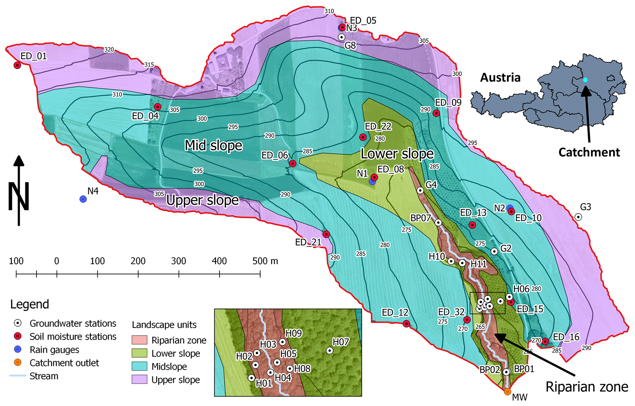
Figure 1 Hydrological Open Air Laboratory in Petzenkirchen, Lower Austria. Coloured areas represent different landscape units defined by the Topographic Position Index (TPI) and terrain slope (riparian zone: TPI ≤ −1; lower slope: −1 < TPI ≤ 0, slope < 5^∘; mid-slope: −1 ≤ TPI ≤ 1, slope > 5^∘; upper slope: TPI > 0, slope ≤ 5^∘). Elevation contour lines with a 5 m interval are given in black. The inset map is the detail of the area marked by a black rectangle on the main map.

The climate is humid with mean annual (2002–2018) precipitation of 781 mm yr⁻¹, air temperature of 9.3 ^∘C, runoff of 170 mm yr⁻¹ and evapotranspiration of 612 mm yr⁻¹ (assuming negligible deep percolation). Investigated years of 2017 and 2018 were dry compared to the long-term (2002–2018) average with 736 and 656 mm of rainfall, respectively. While monthly precipitation peaks in the summer, monthly runoff tends to peak in winter or early spring when the soil moisture and groundwater levels are highest (Széles et al., 2018).

The geology of the area consists of Tertiary fine sediments of the Molasse underlain by fractured siltstone. Seismic measurements show that the layer of mostly non-consolidated deposits is about 200 m thick, except close to the catchment outlet, where the weathered siltstone lies at a depth of about 5 m. Soil core drillings in 2016–2018 show that the predominant soil texture down to 7 m below the surface is silt loam. Based on double-ring infiltrometer measurements on 12 plots in our study area, Picciafuoco et al. (2019) determined a mean saturated hydraulic conductivity of 46.9 and 20.2 mm h⁻¹ for the topsoil in arable land and grassland, respectively. The contact to the lignite sequence lies at a depth of 4 to 36 m below the surface. This sequence is a series of dry, low-conductivity, massive and compact lignite layers interbedded by layers of wet, high-conductivity, and non-consolidated sediments with pebbles. Unpublished pumping test results indicate that these non-consolidated layers have a 10–100 times higher hydraulic conductivity than the overlying silt loams. Based on a soil survey conducted in 2010, the predominant soil types in the top 1 m are Cambisols (57 %), Kolluvisols (16 %), and Planoslols (21 %). Glaysols (6 %) occur close to the stream (Széles et al., 2018).

In the HOAL catchment, a multitude of different runoff mechanisms are observed (Blöschl et al., 2016a). Exner-Kittridge et al. (2016) found that the stream baseflow is mostly due to diffuse groundwater flow directly to the stream or the springs that feed the stream and partly due to the tile drainage discharge. During the rainfall events, saturation excess runoff and infiltration excess runoff occur in the valley bottom during prolonged or intensive rainfall events (Silasari et al., 2017). Part of the event water enters the stream as an overland flow but most infiltrates into the soil matrix and either percolates to the groundwater table or is routed to the stream via tile drains. Macropore flow is observed in summer when the topsoil dries and cracks due to the high clay content (Exner-Kittridge et al., 2016). During rainless periods in the growing season, the diurnal fluctuations of transpiration by the riparian vegetation imprint a diurnal fluctuation on the streamflow, groundwater levels and soil moisture (Széles et al., 2018).

2.2 Data

There are four OTT Pluvio weighing rain gauges distributed throughout the catchment (Fig. 1). They measure precipitation at 1 min intervals and the differences between the stations on the yearly scale do not exceed 5 %. We use the arithmetic mean of precipitation amounts from all four stations as the representative precipitation for the whole catchment.

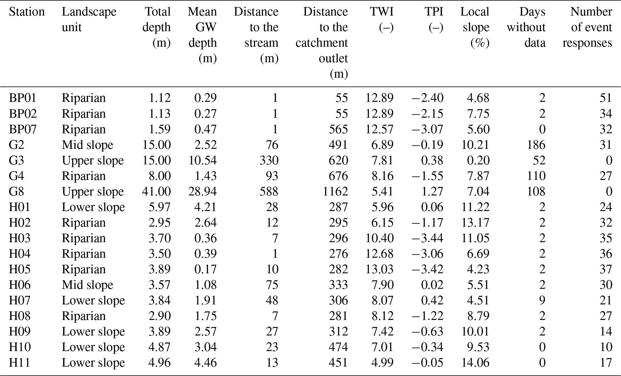
Table 1 Groundwater (GW) measurement stations in the HOAL used in this study. Distance to the stream and the catchment outlet are the distances along the surface flowpath from the GW station's location to the nearest stream reach and catchment outlet, respectively. TWI and TPI are the topographic wetness and topographic position indices, respectively. The last column shows the number of events when a response was observed.

Streamflow at the catchment outlet (MW) (Fig. 1) is routed through an H-flume and continuously measured by a Druck PTX1830 submersible pressure transmitter at a 1 min interval. There are 18 full days and 12 partial days of missing data in 2017–2018 due to measurement device or data transfer malfunction (Fig. 2).

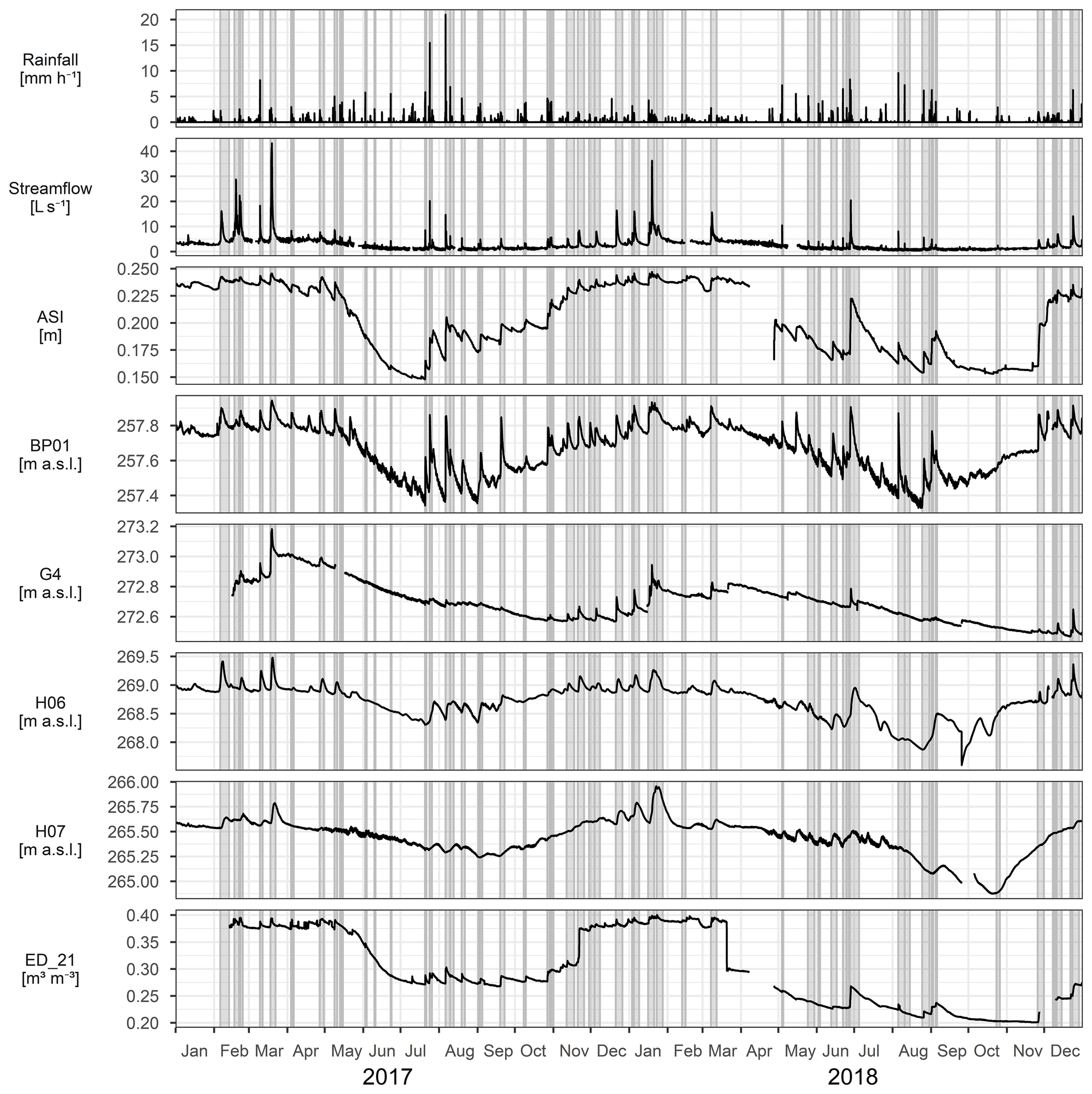
Figure 2 Dynamics of rainfall, streamflow at the catchment outlet, antecedent soil moisture index (ASI), groundwater (BP01, G4, H06, H07) and soil moisture (ED_21) during the investigation period, 2017–2018. The shaded areas represent the times of analysed events.

We use the measurements from 18 groundwater measurement stations, of which 16 are in and around the forested area close to the stream and 2 are at the eastern and northern catchment boundaries, respectively (Fig. 1, Table 1). The stations' depth is between 1 and 41 m and they are screened along the whole depth. Most stations were drilled with a hammering rig to refusal, which usually corresponds to the first consolidated lignite layer's depth. Exceptions are stations G2, G3, G4 and G8, which were drilled into but not through all the lignite layers. All stations are equipped with pressure water level loggers by vanEssen, with a resolution of 0.1 cm H₂O and typical accuracy of 0.5 cm H₂O, which measure at 5 min time intervals. Water level loggers' measurements are barometrically compensated using the atmospheric pressure measured by Baro Diver by vanEssen located close to H11 (Fig. 1). Stations G3, G4 and G8 were only installed in February 2017 and G2 in July 2017, but they are used in the study due to their locations outside the forested area. Other stations only have missing data from 4 to 7 December 2018 due to measurement device failure (Fig. 2).

The soil moisture monitoring network at the study site is equipped with Spade time-domain transmission sensors from Forschungszentrum Jülich, Germany, at four depths below the ground surface (5, 10, 20 and 50 cm) (Blöschl et al., 2016b). For this study, we use 12 permanent stations in the forest, orchards, meadows or field edges and 2 temporary stations in the fields (Fig. 1, Table 2). The temporary stations are removed and reinstalled twice a year following the agricultural practices. Data are collected at an hourly time step. Each sensor at each site is calibrated using the gravimetric method. We obtain the average volumetric soil moisture over a depth of 60 cm following Eq. (1):

$$\begin{array}{}\text{(1)}& \mathit{\theta }=\sum _{i=\mathrm{1}}^{\mathrm{4}}{\mathit{\theta }}_i{\displaystyle \frac{d_i}{D}},\end{array}$$

where θ is the mean volumetric soil moisture content; θ_i is the volumetric soil moisture content at ith sensor and D is the soil column depth (60 cm). d_i is representative column height of the ith sensor determined as the distance between midpoints to the sensor above and below the ith sensor (e.g. d₁ to d₄ are 7.5, 7.5, 20 and 25 cm). Representative columns of the top-most and bottom-most sensors extend up to the ground surface and down to D, respectively. If measurements from one or two sensors are missing, the d_i are adjusted so that working sensors represent more of the soil column.

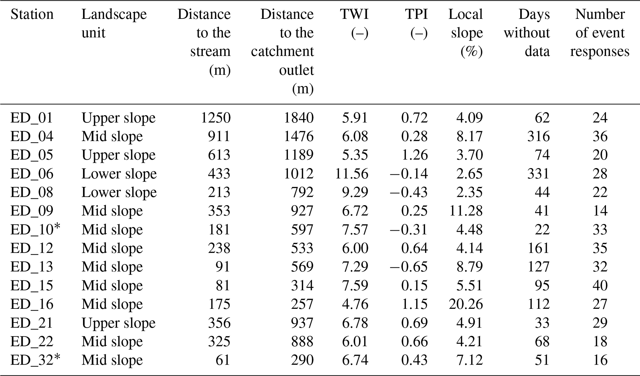
Table 2 Soil moisture (SM) measurement stations and their properties. ^* denotes a temporary station. Distance to the stream and the catchment outlet are the distances along the surface flowpath from the SM station's location to the nearest stream reach and catchment outlet, respectively. TWI and TPI are the topographic wetness and topographic position index, respectively. The last column shows the number of events when a response was observed.

For this study, we use the streamflow at the catchment outlet, groundwater levels, precipitation and soil moisture data from 2017 and 2018. We average the groundwater and streamflow data with the 5 min time step to the 15 min time step and linearly interpolate the soil moisture data from 1 h to the 15 min time step. This time step is small enough to capture the quick responses of streamflow, groundwater, and soil moisture to the precipitation. The streamflow, groundwater levels and soil moisture data are additionally smoothed using the locally estimated scatterplot smoothing (LOESS) as implemented in the R programming language stats package (R Core Team, 2019). This step smooths out the measurement noise and eases the peak detection, which is based on the search for time steps in the time series preceded by consecutive rising and succeeded by consecutive decreasing values. Smoothing might have shifted the peak time by one time step in some cases, which we deem acceptable since most of the peak-to-peak lag times were of orders of hours (see Sect. 3.1.1). We further aggregate the dataset to median weekly values to dampen the event dynamics for the analysis of the seasonal scale. We choose the weekly time step as it is longer than any observed event.

2.3 Site characteristics

To put groundwater and soil moisture responses into the catchment's spatial context, we derive various site characteristics based on the sites' position and the digital elevation model (DEM) with 1 m resolution smoothed with a 10 m by 10 m box filter. For the calculations, we use SAGA GIS (Conrad et al., 2015). First, the local slope and general curvature of the topography are calculated. Upslope catchment area and surface flowpaths are determined from the DEM by the multiple flow direction method (Freeman, 1991). The distance along the surface flowpath from each of the groundwater and soil moisture stations to the nearest stream reach and the catchment outlet is then calculated. The topographic control on local drainage is quantified by the Topographic Wetness Index (TWI) (Beven and Kirkby, 1979), which is calculated by the SAGA wetness index (Böhner and Selige, 2006) module in SAGA GIS.

Slope position is quantified by the Topographic Position Index (TPI) (Weiss, 2001). The TPI compares the elevation of a point and the mean elevation of its surroundings. Points in the valleys have negative and points on the ridges positive TPI values. The TPI can be used for the classification of the landscape into slope position units. We classify our study site with the TPI Based Landform Classification tool in SAGA GIS into four position classes: riparian zone, lower slope, mid slope and upper slope (Fig. 1), with mean TPI values of −2.0, −0.4, 0 and 0.5 and mean slope values of 7.5, 5.0, 6.5 and 4.2^∘, respectively.

2.4 Rainfall-runoff event definition and characterization

We identify 53 rainfall-runoff events during 2017 and 2018 (Fig. 2) that meet all of the following six conditions: (1) significant rainfall is more than 0.1 mm in 15 min; (2) rainfall events are separated by a period of at least 6 h when no significant rainfall occurs; (3) a rainfall event must have the rainfall depth of at least 4 mm; (4) the rainfall-runoff event starts with the rainfall event but continues after the rainfall has stopped for a recession period of 48 h or until a new rainfall event with a rainfall depth of at least 1 mm starts. Selected recession time covers most of the groundwater event dynamics while minimizing the coverage of the stream baseflow fluctuations; (5) no threshold is imposed on streamflow. However, no streamflow data should be missing during the duration of the rainfall-runoff event; (6) at least one groundwater or soil moisture response is found (Sect. 2.5).

For each event, we calculate the following event characteristics. The event duration is the total time between the start and end of the event, as defined above. Rainfall event duration is calculated as time elapsed from the beginning of the event until 90 % of the rainfall amount fell. Rainfall depth is the sum of all precipitation that occurred during the event. The maximum rainfall intensity is the maximum rainfall amount per 15 min interval during the whole event. Change in streamflow (dQ) is the difference between the maximum and minimum streamflow during the event. The streamflow peak time is the elapsed time from the beginning of the event until streamflow reaches its maximum. The runoff depth is the sum of the streamflow, reduced by its minimum, multiplied by the time step (15 min) and divided by the catchment area (66 ha). Following Saffarpour et al. (2016), we use the antecedent soil moisture index (ASI) to measure catchment wetness. We calculate it as the mean volumetric soil moisture content of all soil moisture stations over 24 h before the start of an event multiplied by the soil column depth (0.6 m). A table of all events and their characteristics is in the Appendix (Table A1).

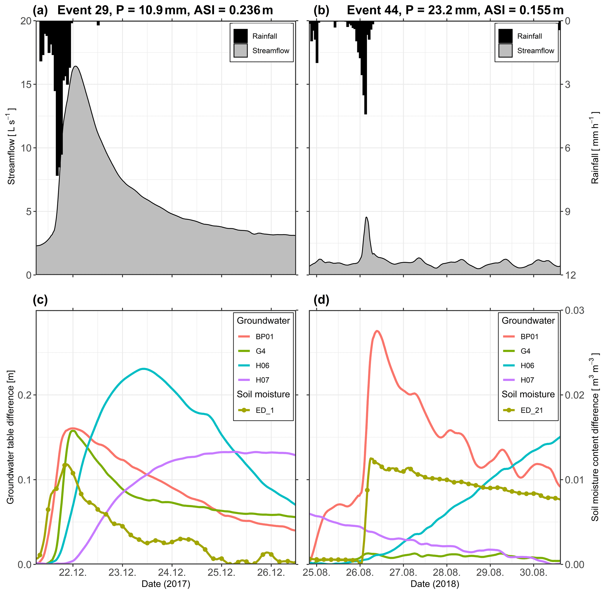
Figure 3 Time series of streamflow at the catchment outlet, rainfall (a, b) and groundwater table (BP01, G4, H06, H07) and soil moisture content (ED_21) (c, d) difference from the event minimum during event 29 (a, c) and event 44 (b, d). P and ASI denote the rainfall depth and antecedent soil moisture index of each of the events, respectively.

2.5 Groundwater and soil moisture event response definition and characterization

We determine whether the groundwater or soil moisture at a station reacted to the precipitation event based on the following rules: (1) stations' event time series must not monotonously rise (Fig. 3d, station H06) or recede (Fig. 3d, station H07), must not be masked by a diurnal signal (Fig. 3d, station BP01) and must have a peak (Fig. 3c). The peak is a point in the time series preceded by at least 24 time steps of increasing and at least 4 time steps of decreasing values. If more peaks are detected, the one closest to the time of the streamflow peak is selected. (2) The minimum change in the groundwater table and soil moisture content is 5 mm and 0.005 m³ m⁻³, respectively. The change is calculated as the difference between the value at the peak and the minimal value before it. We also determine local antecedent conditions as the mean groundwater table or soil moisture 1 h before the event for each response.

During the 53 rainfall-runoff events, we observed a total of 458 groundwater responses to the precipitation at 15 stations and 374 soil moisture responses at 14 stations. We adopt three event descriptors: Spearman correlation coefficient, hysteresis index, and peak-to-peak time for the comparison of these responses. We choose these three because they are easy to understand, suitable for all variables whose responses are due to the same driver and transferable to other catchments.

Figure 4 Weekly median time series of streamflow at the catchment outlet (MW) and the groundwater table (BP01, G4, H06, H07) and the soil moisture content (ED_21) difference from the minimum for the years 2017–2018.

Hysteresis loops have been demonstrated as a simple but insightful method for investigating the relationships between streamflow and other hydrological or chemical variables (Allen et al., 2010; Fovet et al., 2015; Scheliga et al., 2018). We can obtain a hysteresis loop if we plot concurrent values of two variables against each other. The hysteresis index (HI) describes the size and rotational direction of such a loop. Various definitions of the HI have been proposed in hydrology (Aich et al., 2014; Langlois et al., 2005; Lawler et al., 2006; Lloyd et al., 2016; Zuecco et al., 2016). In this study, we use a definition similar to Lloyd et al. (2016) and Zuecco et al. (2016). The input time series (e.g. streamflow, groundwater level, soil moisture) are first normalized to values between 0 and 1 by the range of values for a specific event. The HI is then calculated as the integral of the loop of the two normalized variables plotted against each other. The resulting HI ranges between −1 and 1, where the magnitude describes the loop's shape and the sign the rotational orientation. The wider the loop, the greater the absolute HI value. Clockwise loops, where the variable on the vertical axis peaks first, have positive HI values. The anticlockwise loops, where the variable on the horizontal axis peaks first, have negative HI values. A detailed explanation of the HI calculation is in Appendix B.

Peak-to-peak time is the time difference between the peak time of the first and second variables. Peak-to-peak times to streamflow are positive if the streamflow peaks first and negative if the other variable peaks first.

To describe the similarity between streamflow, groundwater and soil moisture seasonal dynamics, we also use three descriptors, i.e. Spearman correlation coefficient, hysteresis index and time shift in seasonal dynamics. The latter differs from the peak-to-peak time calculated on the event scale. Seasonal time shift is the lag time when the cross-correlation of two variables is the highest. For these calculations, the weekly median of streamflow, groundwater levels and soil moisture content are used to smooth out the event dynamics (Fig. 4). Only stations with more than 45 weeks of data in a year are used. Because of data gaps, station ED_32 is left out entirely, stations G2–G4, ED_09 and ED_10 are left out for the year 2017 and stations ED_08 and ED_22 are left out for the year 2018.

For the analysis of spatial patterns, we calculated the median value of the three descriptors for each station pair over all events and both years. We investigate the temporal patterns in terms of changing wetness conditions, which can only be done on the event scale. For that, we use the comparisons of groundwater and soil moisture event responses to streamflow and aggregate them by landscape units and the sum of ASI and total rainfall. The entire analysis is done with the R programming language (R Core Team, 2019). Statistical significance is assessed by p values calculated using the t-distribution approximation as implemented in the stats package.

2.6 Classification of event responses

To investigate the control of site and event characteristics on the connectivity on the event scale, we first classify the relationship between the streamflow event response to the groundwater and soil moisture event response into response types. The classification is based on the event descriptors (Spearman correlation coefficient, hysteresis index and peak-to-peak time) and performed by combining the hierarchical clustering analysis and classification trees. An additional benefit of response types compared to the adopted descriptors is potentially better transferability to other catchments with for example more conductive soils.

Hierarchical clustering is a method of identifying groups of similar data points in a dataset. We use the descriptors mentioned above of groundwater event responses from all observed events at all available stations as the input dataset variables. Only groundwater responses are used in this step because they have greater variability of descriptor values than soil moisture responses. The clustering is performed with Ward's hierarchical clustering algorithm (Murtagh and Legendre, 2014) implemented in the stats package in the R programming language (R Core Team, 2019), which gives us three clusters of similar size.

A disadvantage of hierarchical clustering is a lack of specific rules that could be used to classify additional hydrological variables or datasets from other catchments. That is why we do an extra step and use the information gained from clustering to construct a discrete decision tree, also known as a classification tree. The cluster number is used as a dependent and the three event descriptors are used as independent variables in the input dataset for the classification tree algorithm implemented in R package rpart (Therneau and Atkinson, 2019). The resulting three-node classification tree is shown in Fig. 5. It allows us to determine the type of relationship between two responses with the precipitation event, based only on the hysteresis index and Spearman correlation coefficient. The difference between the response type determined by the clustering and by the classification tree is less than 6 %. This classification tree is also used here to classify the soil moisture responses to precipitation events in relation to streamflow.

Figure 5 Decision tree for the classification of groundwater responses in relation to the streamflow responses to precipitation events into three response types. Responses are split based on the hysteresis index (HI) and Spearman correlation coefficient (Cor), as shown by the expressions on the horizontal lines between nodes. Each node is coloured based on the predominant response type, while the colour intensity denotes the purity of the classification. Node text shows the predominant response type, the percent of responses of each type at that node in the input database (IN) and the percent of the total number of responses at that node (OUT).

We assess how site and event characteristics affect the connectivity on the event scale by looking at how they correlate with response types. We calculate the Pearson correlation coefficient between each response type's frequency to the site characteristics of each station. We also calculate the correlation between each response type's frequency for each event to the event characteristics for groundwater and soil moisture stations. We deem correlations with p<0.05 to be significant.

3 Results

3.1 The similarity of groundwater, soil moisture and streamflow event responses

3.1.1 Spatial patterns

We find spatial patterns in the median event Spearman correlation coefficients between groundwater responses and streamflow response (Fig. 6). The riparian stations BP01, BP02, BP07, H04, H05 and G4 have the highest mean Spearman correlation with the streamflow (r_s>0.6). Correlation is lower in other groundwater stations. All of the soil moisture stations have mostly moderate correlations with streamflow ($\mathrm{0.3}<r_{\mathrm{s}}<\mathrm{0.5}$). The similarity among the stations in the same landscape unit is comparable to the similarity to streamflow. The riparian zone groundwater stations (Fig. 6, red rectangle) have the highest Spearman correlation coefficients among them ($\stackrel{\mathrm{‾}}{r_{\mathrm{s}}}=\mathrm{0.75}$). Correlations among the lower-slope and mid-slope stations are lower, and they are also not well correlated with other stations. Exceptions are station H11, positioned above the stream valley, but it is very close to the stream, and station G2, located far from the stream but in an always wet location. Overall, the soil moisture stations are well correlated among themselves ($\stackrel{\mathrm{‾}}{r_{\mathrm{s}}}=\mathrm{0.69}$) and moderately correlated with the riparian groundwater stations. Upper-slope soil moisture stations have a lower correlation among them and with other stations compared to the average for the soil moisture stations.

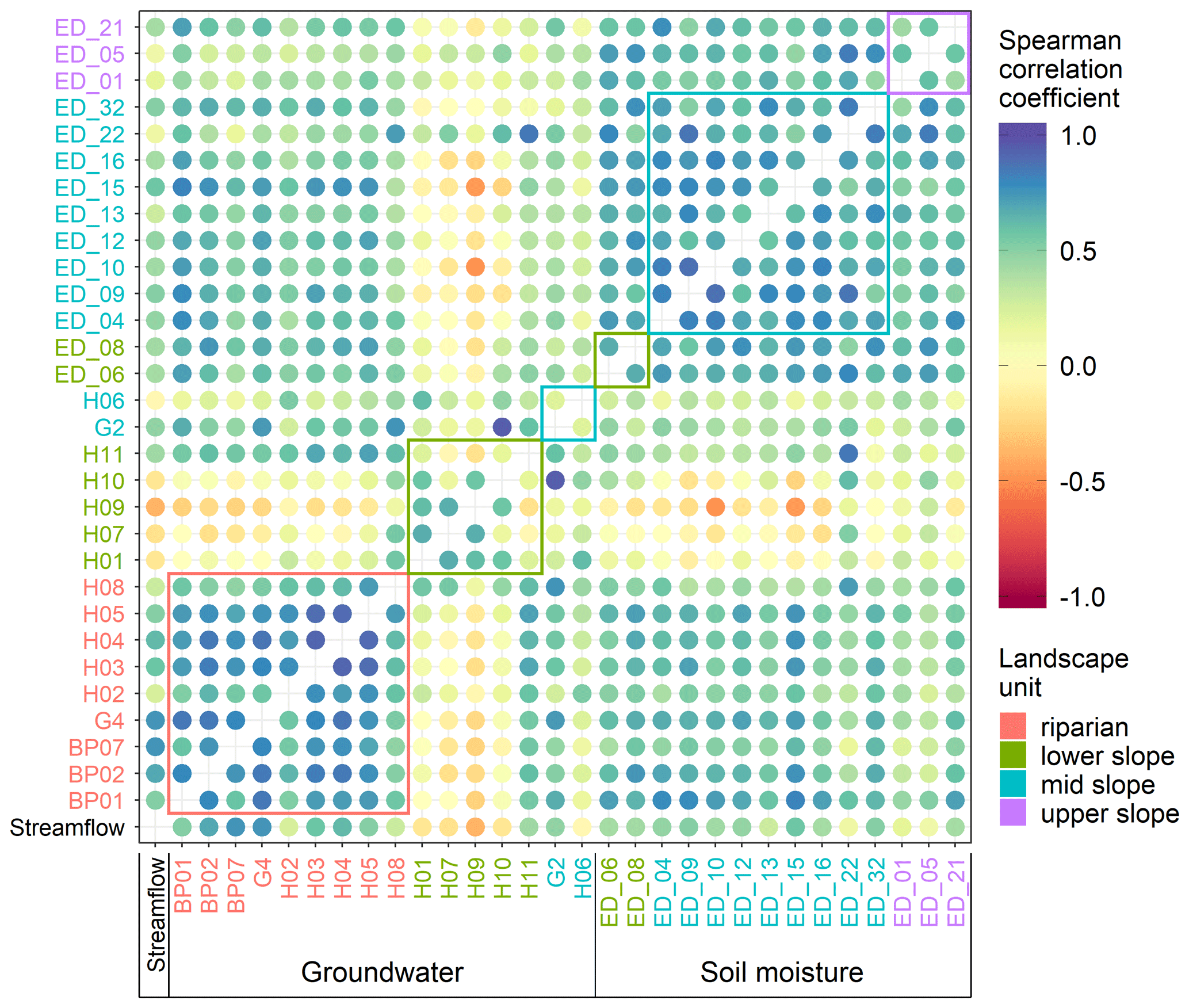
Figure 6 Median Spearman correlation coefficient between streamflow at catchment outlet (streamflow), groundwater stations (BP^*, H${}^{**}$, G^*) and soil moisture stations (ED_${}^{**}$) for all events. The circles' colour corresponds to the Spearman correlation coefficient. The station names' colour corresponds to their landscape unit. Coloured rectangles enclose correlations of stations in the same landscape unit.

The median event hysteresis indices between streamflow, groundwater and soil moisture event responses show similar spatial patterns (Fig. 7) as the median event Spearman correlation coefficient. Where the Spearman correlation coefficient is high, the hysteresis index is closer to zero, and where the coefficient is low, the absolute value of the hysteresis index is high. Most of the hysteresis indices of groundwater and soil moisture responses against streamflow responses are negative (Fig. 7, first column). This indicates that, on average, the hysteresis loops are anticlockwise and streamflow responds to precipitation (Fig. 8, first column) quicker than groundwater and soil moisture do.

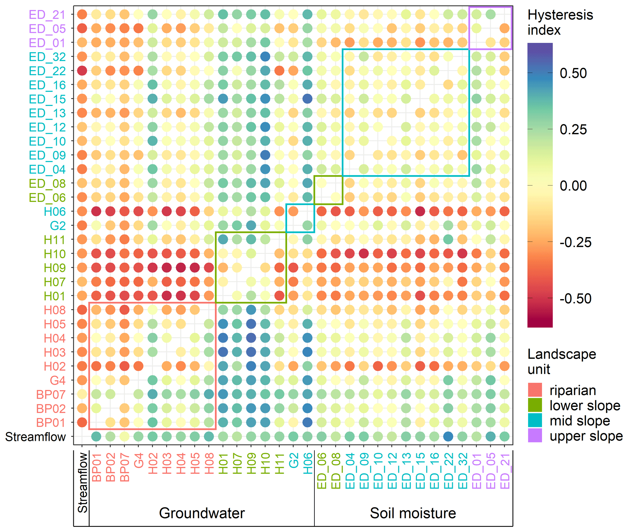
Figure 7 Median hysteresis index between streamflow at catchment outlet (streamflow), groundwater (BP${}^{**}$, H${}^{**}$, G^*) and soil moisture (ED_${}^{**}$) for all events. Hysteresis index is positive if the row station peaks before the column station and negative if the row station peaks after the column station. Circles' colour corresponds to the value of the hysteresis index. The station names' colour corresponds to their landscape unit. Coloured rectangles enclose values of stations in the same landscape unit.

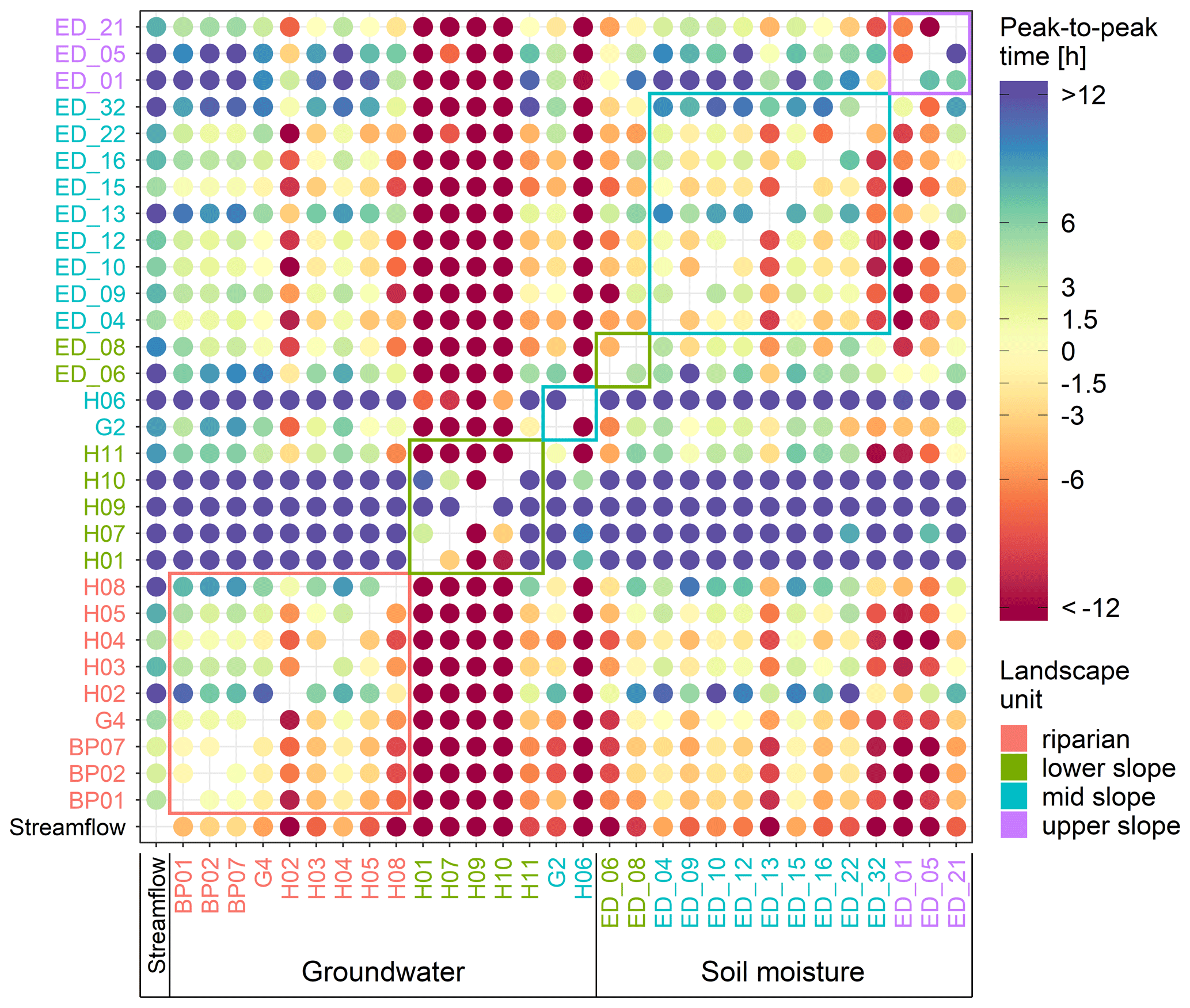
Figure 8 Median peak-to-peak time between streamflow at catchment outlet (streamflow), groundwater (BP${}^{**}$, H${}^{**}$, G^*) and soil moisture (ED_${}^{**}$). Time is positive if the row station peaks before the column station and negative if the row station peaks after the column station. Circles' colour corresponds to the value of the peak-to-peak time. The station names' colour corresponds to their landscape unit. Coloured rectangles enclose values of stations in the same landscape unit.

Spatial patterns in median event peak-to-peak times (Fig. 8) confirm the assessment based on the hysteresis index (Fig. 7, first column). On average, groundwater and soil moisture peak later than streamflow. Further, Fig. 8 reveals details that are not so clearly visible in the median event correlation and hysteresis index. The upper-slope soil moisture stations peak later than other soil moisture stations. We see also that groundwater stations H02 and H08 are different to the rest of the riparian stations and are more like the lower-slope stations, which is probably due to their deeper groundwater table compared to the rest of the riparian stations.

On average, groundwater and soil moisture at all stations peak 15±21 and 9±14 h (mean and standard deviation) after streamflow, respectively (Fig. 8, first column). The lowest peak-to-peak times between streamflow and groundwater were observed in the riparian zone (median 2.7±14 h). There, in some instances, groundwater even peaked before streamflow (Figs. A1c and 9f). The Pearson correlation coefficient between the event response Spearman correlation coefficient and TWI (Fig. A1a) and TPI is ρ=0.38 and $\mathit{\rho }=-\mathrm{0.45}$, respectively. Pearson correlation coefficient between the peak-to-peak time and TWI (Fig. A1c) and TPI is $\mathit{\rho }=-\mathrm{0.42}$ and ρ=0.51, respectively. In other words, groundwater event responses towards the valley bottom, where the contributing area is greater and the groundwater table is shallower, are increasingly more similar to the streamflow responses. The peak-to-peak times between them are decreasing. The soil moisture event response descriptors do not correlate with the site characteristics (Fig. A1).

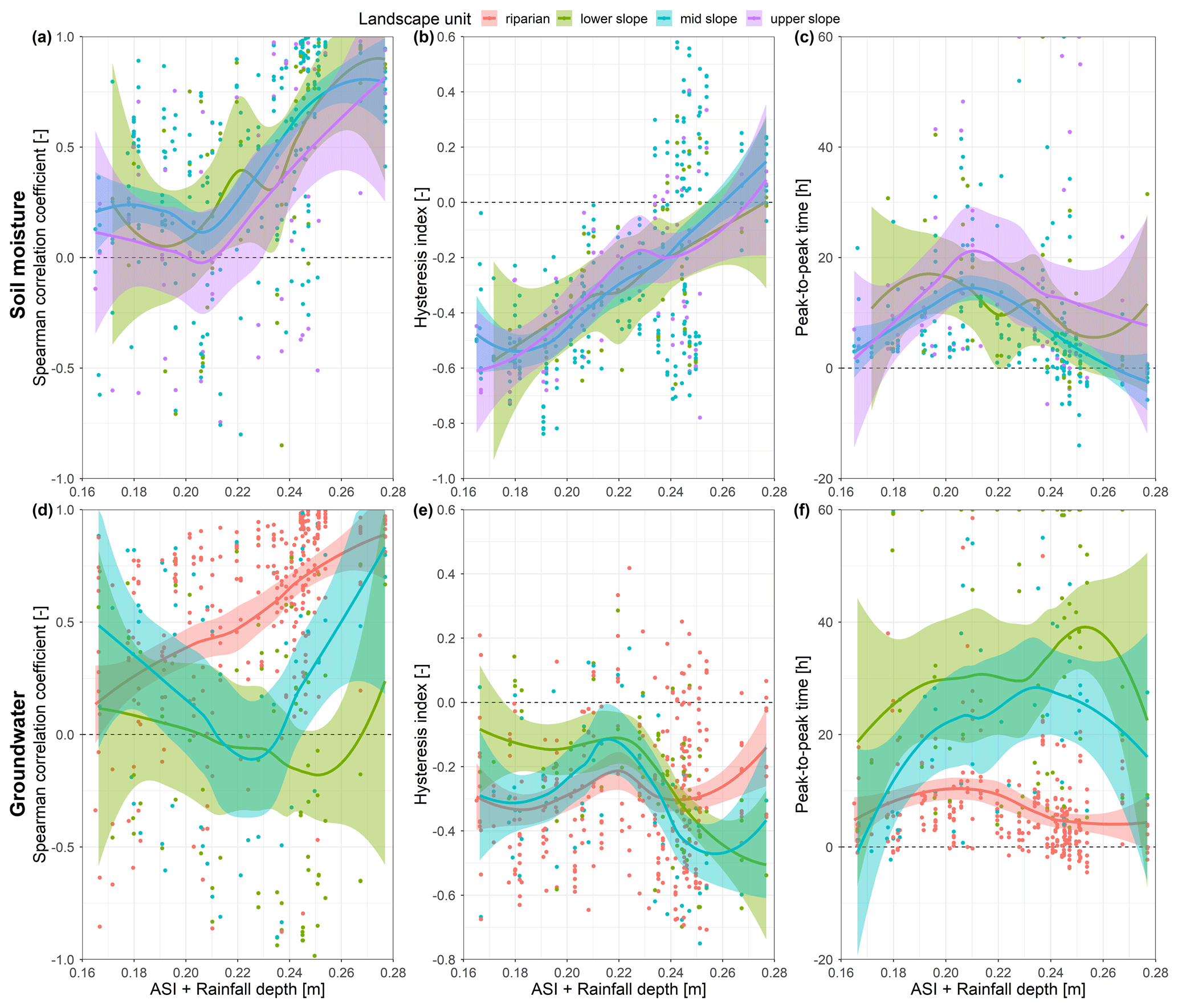
Figure 9 Spearman correlation coefficient (a, d), hysteresis index (b, e) and peak-to-peak time (c, f) of soil moisture (a–c) and groundwater (d–f) responses to streamflow event responses over changing event catchment wetness conditions (ASI + rainfall depth). Colours represent different landscape units. Points are calculated values for each available response. Lines are local regression fits for each landscape unit and shaded areas the corresponding 95 % confidence intervals.

3.1.2 Temporal patterns through wetness conditions

While there is small spatial variability of descriptors for soil moisture responses in relation to the streamflow, the pattern changes in time with the catchment wetness (ASI + rainfall depth) (Fig. 9, top row). Spearman correlation coefficient and the hysteresis index increase with the increasing wetness (Pearson correlation of ρ=0.45 and ρ=0.57, respectively). The trend of peak-to-peak time is nonlinear in the shape of an inverted parabola (Fig. 9c), with the longest times at medium wetness conditions. These three trends are very similar for all landscape units. The small dip in correlation and increase in peak-to-peak times during medium wetness conditions might indicate that different flowpaths activate during the dry and wet conditions.

Trends of groundwater event response descriptors with the wetness conditions differ for each landscape unit (Fig. 9, bottom row). Spearman correlation coefficient steadily increases with increasing wetness in the riparian zone (Fig. 9d). At the same time, there is no clear trend in the lower slope and a parabolic trend in the mid slope, probably due to a deeper groundwater table. Trends of hysteresis index and peak-to-peak time are not so clear. Peak-to-peak times are shorter in the riparian zone compared to other landscape units. They also seem to shorten with the increasing wetness, which is coherent with the increasing correlation. Peak-to-peak times in the mid slope are lower than in the lower slope, which is again coherent with the Spearman correlation coefficient. Trends of Spearman correlation coefficient and peak-to-peak time suggest that the control of the wetness conditions is related to the mean groundwater depth in the landscape unit. Trends are the clearest in the riparian zone, where the groundwater table is the shallowest, followed by the mid slope and lower slope, which has the deepest groundwater table.

In the vast majority of cases, groundwater peaks after the streamflow (Fig. 9). During wet conditions (ASI + rainfall depth > 0.23), there are many stations in the riparian zone that peak before. This difference probably indicates that most of the time, flowpaths bypassing the groundwater (monitoring stations) feed the event streamflow. Only when the catchment wetness is sufficiently high does the riparian zone contribute to the event streamflow.

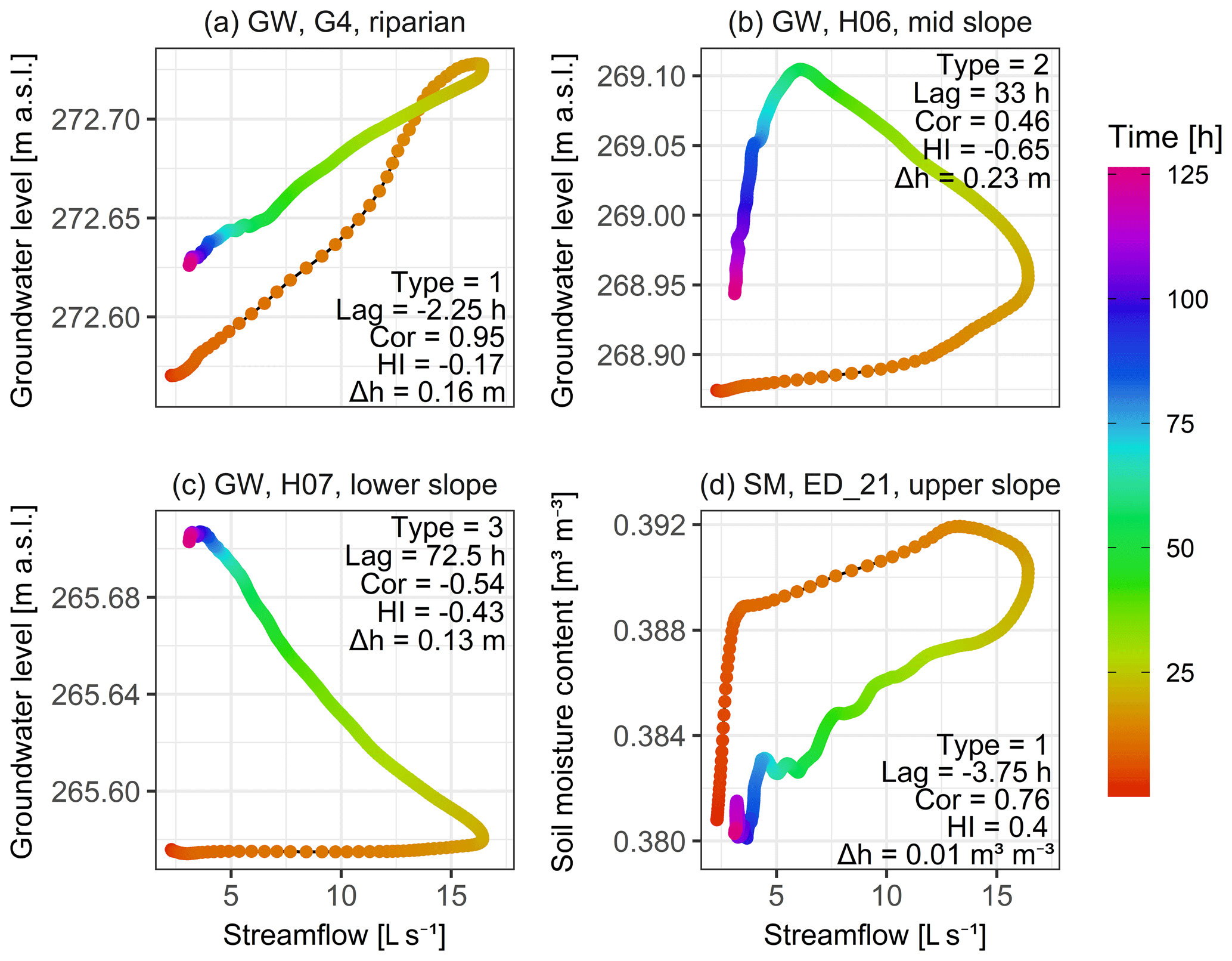
Figure 10 Hysteresis loops for event 29 (31 December 2017) (Fig. 3c). Each panel represents a different response type: (a) type-1 groundwater (GW) response; (b) type-2 GW response; (c) type-3 GW response; (d) type-1 soil moisture (SM) response. The points' colour represents the time since the start of the event. Event dynamics of each station in relation to the streamflow is described by the response type (Type), peak-to-peak time (Lag), Spearman correlation coefficient (Cor), hysteresis index (HI) and groundwater table or soil moisture content change over the event (Δh).

3.2 Event response types

3.2.1 Event response classification

Altogether we determined 170, 203 and 85 groundwater responses and 136, 183 and 55 soil moisture responses in relation to the streamflow of type 1, type 2 and type 3, respectively. Response types represent different levels of similarity between the groundwater or soil moisture to the streamflow, as follows.

• Type-1 responses have a hysteresis index between −0.3 and 0.58 and a Spearman correlation coefficient between 0 and 0.99. These were groundwater and soil moisture responses that were similar to the streamflow response. The hysteresis loop was narrow, the lag time was short, and the groundwater table or soil moisture content have increased and decreased on the same timescale as the discharge (Fig. 10a and d).

• Type-2 responses had a hysteresis index between −0.84 and −0.3 and a correlation coefficient between −0.2 and 0.96. Typical for these response types are wide hysteresis loops. The rising limb of the groundwater or soil moisture event time series is relatively long but still overlaps with the streamflow hydrograph's rising and receding limb (Fig. 10b).

• Type-3 responses either had a hysteresis index between −0.64 and 0.16 or a correlation coefficient between −0.98 and 0. These groundwater and soil moisture responses were least correlated with streamflow. Their rising limb either started late after the start of the rainfall or continued to increase past the end of event time (Fig. 10c).

3.2.2 Spatial patterns of event response types

The spatial patterns of hysteresis index, Spearman correlation coefficient and peak-to-peak times (Sect. 3.1.1) propagate to the pattern of event response type co-occurrence (Fig. 11). Event response type co-occurrence is the frequency of events when two stations have the same type of response. Apart from the riparian zone, where the co-occurrence rate is 64 % ± 15 % between stations, the other two landscape units show only low co-occurrence rates of groundwater response types between stations in the same unit. The highest co-occurrence rate is observed between the three piezometers H03, H04 and H05. These stations respond with the same response type in more than 85 % of the events. Their co-occurrence rate with piezometers downstream (BP01, BP02) and upstream (BP07) is also high (68 %–84 %), indicating that the distance to the stream is more important than the position along the stream. Riparian zone piezometers have a reasonable response type co-occurrence rate with the soil moisture stations (62 % ± 14 %). Soil moisture stations, with some exceptions, have high co-occurrence rates regardless of the landscape unit (mean 78 % ± 11 %).

Figure 11 The frequency of events when two stations have the response of the same type – i.e. response-type co-occurrence. The size of circles corresponds to the number of events when both stations had a response. Circles' colour corresponds to the frequency of the response-type co-occurrence. The station names' colour corresponds to their landscape unit. Coloured rectangles enclose values of stations in the same landscape unit.

Figure 12 Seasonal hysteresis loops of three groundwater stations (a–c) and one soil moisture station (d) to the streamflow for the year 2018 (Fig. 4). Circles' colour represents the week of the year. Seasonal dynamics of each station in relation to the streamflow is described by seasonal shift (Lag), Spearman correlation (Cor), hysteresis index (HI) and groundwater table elevation or soil moisture content change over the year (Δh).

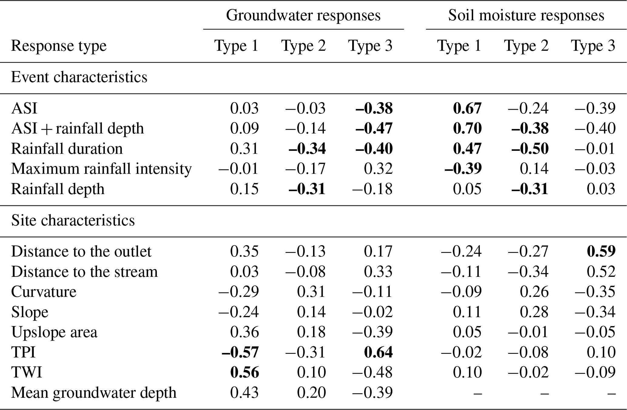
3.2.3 Spatial and temporal controls of event response types

We observe the clearest trend in the groundwater response-type frequency with the TPI and the TWI (Table 3). The frequency of the type-1 responses decreases, and the frequency of the type-3 responses increases with the TPI increase and the TWI decrease (Fig. A2a). This trend means that groundwater in the valley bottom reacts more like streamflow than on the slopes and ridges. The response-type frequency by landscape units further corroborates this result. The type-1 frequency is more than 43 % in the riparian zone and only 22 % and 18 % in the lower and mid slopes, respectively. The highest frequency of type-3 responses is at the lower slope (50 %), while it is lowest in the riparian zone (7 %). The soil moisture response-type frequencies do not vary considerably with the TPI or the TWI (Fig. A3a) but rather with the distance from the stream and the catchment outlet and less pronounced with the terrain curvature and slope (Table 3). Soil moisture responses are less similar, i.e. frequency of type-3 increases, further from the stream or catchment outlet and where the curvature and slope of the terrain are smaller.

Figure 13 Median Spearman correlation coefficient between median weekly streamflow at catchment outlet (Q), groundwater (BP${}^{**}$, H${}^{**}$, G^*) and soil moisture (ED_${}^{**}$) over years 2017 and 2018. Circles' colour corresponds to the value of the Spearman correlation coefficient. The station names' colour corresponds to their landscape unit. Coloured rectangles enclose values of stations in the same landscape unit. Only time series longer than 45 weeks per year are compared.

Soil moisture response-type frequencies are correlated the strongest with the catchment wetness (ASI, ASI + rainfall depth) (Table 3). With increasing wetness, the similarity of soil moisture responses to the streamflow also increases (Fig. A3b). This correlation is weaker for the frequency of groundwater response types. The frequencies of both groundwater (Fig. A2c) and soil moisture (Fig. A3c) response types are correlated with the rainfall duration (Table 3). The responses are more similar to streamflow when the events are longer, i.e. less intensive.

Table 3 Pearson correlation coefficient of site and event characteristics with the frequency of different event response types of groundwater and soil moisture in relation to the streamflow. ASI is the antecedent soil moisture index. TPI and TWI are topographic position index and topographic wetness index, respectively. The significance of correlations was tested with t-distribution approximation and correlations with p<0.05 are shown in bold.

3.3 Similarity of groundwater, soil moisture and streamflow seasonal dynamics

Examples of the seasonal hysteresis loops of the stations G4, H06, H07 and ED_21 are shown in Fig. 12. Shapes of loops in Fig. 12a–c are different from corresponding event loops in Fig. 10, indicating a difference in the similarity in the seasonal and event dynamics of these stations to the streamflow. We see further differences between the median seasonal Spearman correlation coefficients (Fig. 13), hysteresis index (Fig. 14) and time shift (Fig. 15) to their counterparts on the event scale (Figs. 6–8).

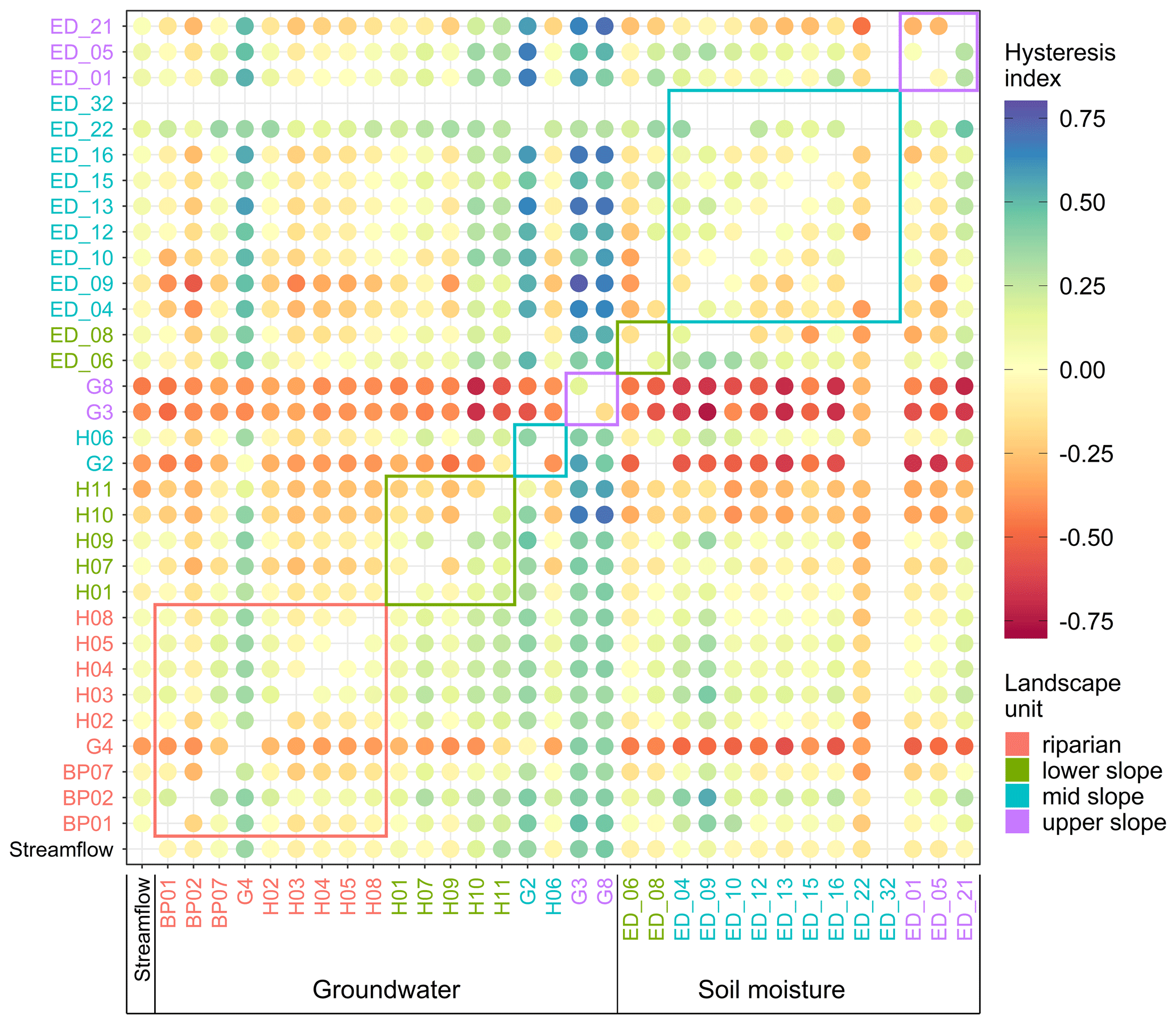
Figure 14 Median hysteresis index between median weekly streamflow at catchment outlet (Q), groundwater (BP${}^{**}$, H${}^{**}$, G^*) and soil moisture (ED_${}^{**}$) over the years 2017 and 2018. Hysteresis index is positive if the row station peaks before the column station and negative if the row station peaks after the column station. Circles' colour corresponds to the value of the hysteresis index. The station names' colour corresponds to their landscape unit. Coloured rectangles enclose values of stations in the same landscape unit. Only time series longer than 45 weeks per year are compared.

The Spearman correlation coefficient of groundwater and soil moisture seasonal dynamics to the streamflow (Fig. 13) is, in contrast to the event scale, high (ρ>0.7) for all stations except G2 (ρ=0.63), G3 (ρ=0.14), G4 (ρ=0.63) and G8 (ρ=0.07). Surprisingly, the lower- and mid-slope groundwater stations with a low correlation with streamflow on the event scale show a high correlation on the seasonal scale. Two examples are stations H01 and H06, with mean event correlations with streamflow of $\mathit{\rho }=-\mathrm{0.15}$ and $\mathit{\rho }=-\mathrm{0.04}$ and seasonal correlations of ρ=0.93 and ρ=0.89, respectively. Correlation among stations in the same landscape unit is highest in the riparian zone, also on the seasonal scale. Still, the difference to other landscape units is smaller compared to the event scale. Even upper-slope groundwater stations, which do not correlate well with stations in other landscape units, are well correlated with each other. All soil moisture stations are well correlated with the stream ($\stackrel{\mathrm{‾}}{r_{\mathrm{S}}}=\mathrm{0.83}\pm \mathrm{0.06}$) and among them in all landscape units.

The seasonal- and event-scale patterns are more similar for the median hysteresis index (Fig. 14) than the Spearman correlation coefficient. Riparian station G4 and some lower-, mid- and upper-slope groundwater stations have a negative hysteresis index against the streamflow (Fig. 14, first column), indicating a delay in their seasonal dynamics. These are stations with the deepest groundwater table, and some are also in contact with the deep groundwater system. All soil moisture stations have a hysteresis index in relation to the streamflow close to zero or even slightly positive, indicating mostly synchronous seasonal dynamics.

Seasonal dynamics of streamflow, groundwater and soil moisture in the research area is roughly sinusoidal, with the highest values in winter and the lowest in summer. The seasonal dynamics shift time tells us how much out of phase the dynamics of two stations are. Figure 15 shows that the dynamics of stations G2, G3, G4 and G8 are delayed compared to the streamflow by 56, 91, 49 and 70 d, respectively. On the other hand, some soil moisture stations show slightly early dynamics, which indicates that soil moisture conditions drive the seasonal dynamics of streamflow and partly groundwater.

Table 4 Pearson correlation coefficient between site characteristics and the Spearman correlation, hysteresis index and time shift of groundwater and soil moisture seasonal dynamics in relation to streamflow. TPI and TWI are topographic position index and topographic wetness index, respectively. Significance of correlations was tested with t-distribution approximation and correlations with p<0.05 are shown in bold.

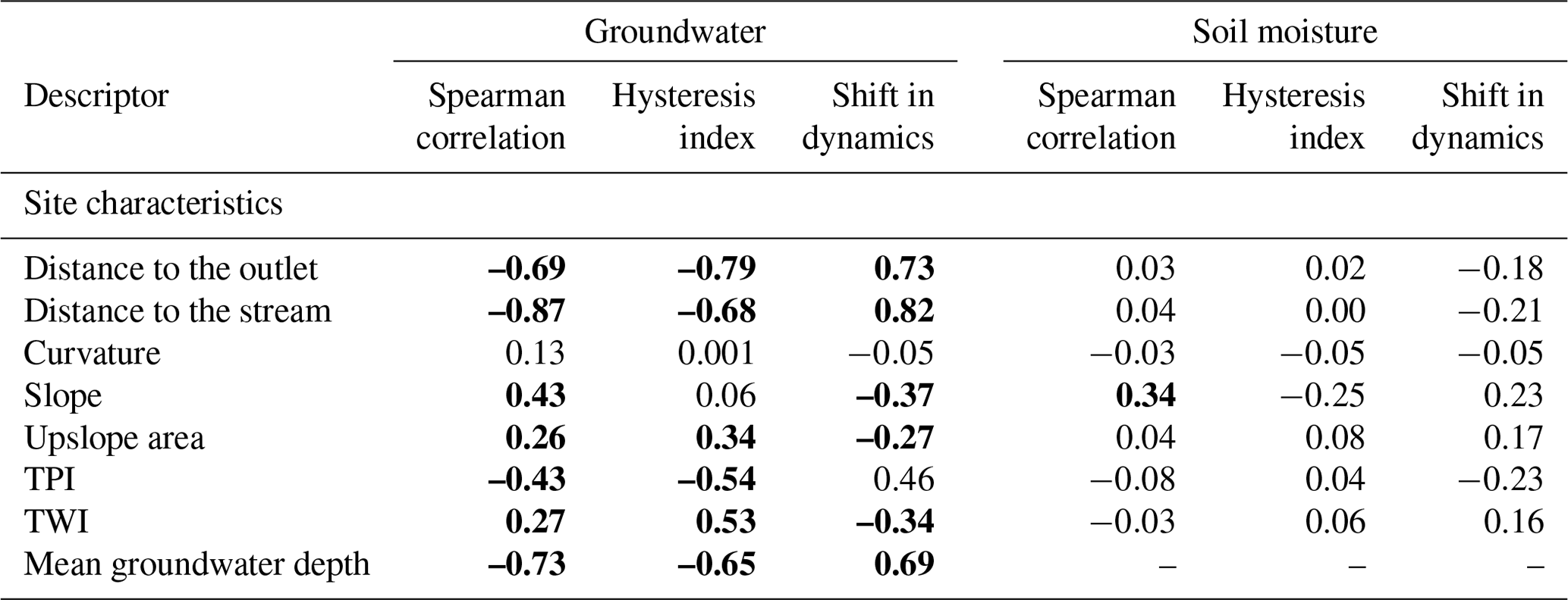
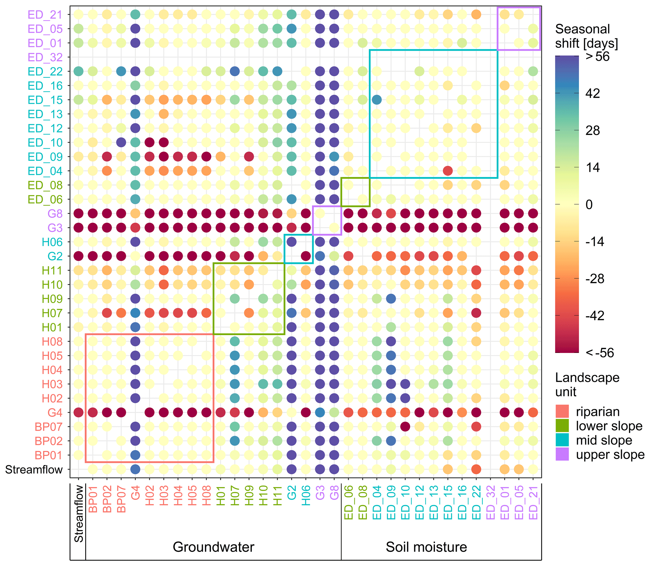
Figure 15 Median seasonal shift between median weekly streamflow at catchment outlet (Q), groundwater (BP${}^{**}$, H${}^{**}$, G^*) and soil moisture (ED_${}^{**}$) over the years 2017 and 2018. The seasonal shift is positive if the row station's seasonal maxima and minima occur before the maxima and minima of the column station and vice versa. Circles' colour corresponds to the value of the seasonal shift. The station names' colour corresponds to their landscape unit. Coloured rectangles enclose values of stations in the same landscape unit. Only time series longer than 45 weeks per year are compared.

The spatial homogeneity of the seasonal soil moisture dynamics is reflected in a weak correlation between the site characteristics (Table 4) and the three descriptors, similar to what we also see on the event scale. Groundwater seasonal descriptors, on the other hand, are well correlated with most site characteristics. Distance to the stream has the highest correlation with all three descriptors, followed by the distance to the outlet and mean groundwater table depth. Spearman correlation coefficient between the groundwater and streamflow seasonal dynamics decreases with the increasing distance to the stream and the catchment outlet and depth to the groundwater table. In other words, stations closer to the stream with a shallower groundwater table, i.e. riparian stations, have responses more similar to the streamflow, while stations on the catchment border with a deep groundwater table, i.e. upper-slope stations, are more different.

4 Discussion

4.1 Spatial and temporal patterns of groundwater and soil moisture responses to precipitation

In this study, we investigate patterns of the connectivity between streamflow, groundwater and soil moisture. We assess the connectivity as the similarity between two responses to the same precipitation event given by the Spearman correlation coefficient (Fig. 6), hysteresis index (Fig. 7), peak-to-peak times (Fig. 8) and as all three aggregated into a response type (Fig. 11). The similarity between different groundwater stations and between groundwater and streamflow event dynamics shows spatial organization related to the landscape units.

The highest similarity between the groundwater and streamflow event dynamics is observed in the riparian zone. There the groundwater table is closest to the surface and the soil water deficit is small throughout the year, indicating that the riparian zone is continuously connected to the stream. Upslope from the stream, the similarity is lower (Figs. 6 and 7), suggesting lower connectivity to the stream than in the riparian zone. We attribute that to the deeper groundwater table compared to the riparian stations, based on the positive Pearson correlation of peak-to-peak times and the depth to the mean groundwater table (Sect. 3.2.1). Greater groundwater depth equals more available storage in the unsaturated zone and a longer percolation path, both leading to later peak time. Another possible explanation for the lower connectivity upslope from the stream is that most water perched above the impeding lignite layer percolates through it before reaching the stream (Gabrielli and McDonnell, 2020; Klaus and Jackson, 2018).

Anticlockwise hysteresis loops (Fig. 7 first column, Fig. 9e) and positive peak-to-peak times (Fig. 8 first column, Fig. 9f) between streamflow and groundwater event responses indicate that during the majority of events, groundwater does not directly contribute to the event runoff or it does so only during the falling limb of the hydrograph. Event water, contributing to the rising limb of the hydrograph, probably bypasses the groundwater via surface flow, tile drains or other subsurface preferential pathways. Only riparian groundwater seems to contribute to the rising limb of the hydrograph, as is suggested by the negative peak-to-peak times and positive hysteresis index (Fig. 9f and e) for some events (e.g. BP01 and G4 in Fig. 3c).

Other studies have found similar spatial patterns of groundwater event dynamics in humid headwater catchments. Haught and Van Meerveld (2011) reported that streamflow and groundwater event responses were significantly better correlated in the footslope up to 8 m from the stream than in the hillslope further away from the stream. They concluded that a strong correlation together with short negative lag times suggest that transient groundwater in the lower hillslope contributes to event runoff. A similar difference between the riparian zone and the hillslope was reported by Scheliga et al. (2018) and Fovet et al. (2015). They observed mostly anticlockwise hysteresis loops between streamflow and the deeper groundwater on the hillslopes and clockwise hysteresis loops in the valley bottom, reflecting the spatial difference in the availability of storage in the soils and groundwater system, which is high on the hillslope and lower in the riparian zone.

The similarity pattern changes with wetness conditions (Fig. 9). The similarity of groundwater to streamflow in the riparian zone increases with wetness. On the hillslope, the peak-to-peak times are the shortest and the Spearman correlation coefficients are the highest during very dry and very wet conditions, indicating the change in active flowpaths. In summer months during dry conditions, the soils in the HOAL were observed to crack (Blöschl et al., 2016a), enabling the water to infiltrate faster and, during the wet conditions, the hydraulic conductivity increases due to the lower soil water deficit in both cases facilitating connectivity to the stream. Findings from other headwater catchments suggest that groundwater connectivity to the stream increases with increasing catchment wetness conditions. This connectivity increase could manifest as the decrease in peak-to-peak lag times between hillslope groundwater and streamflow (Haught and Van Meerveld, 2011; Lana-Renault et al., 2014), higher groundwater peaks (Detty and McGuire, 2010) and fraction of activated wells (Penna et al., 2015).

We observed high variability of response dynamics between the lower- and mid-slope stations. Even stations just a few tens of metres apart, e.g. H04 and H02, could show different responses. This agrees with the short characteristic length scales of similarity found between the groundwater and streamflow event dynamics in a pre-Alpine Swiss catchment (Rinderer et al., 2017). Also, groundwater event responses observed at the Bridge Creek Catchment in the Italian Dolomites could distinctly differ in magnitude and timing just a few metres apart (Penna et al., 2015).

We do not observe any spatial patterns in the similarity between the soil moisture and streamflow event responses, and most of the soil moisture stations react similarly to each other (Fig. 11). A reason for this homogeneity might be the small variability of topsoil texture (Blöschl et al., 2016a), local terrain slope and curvature (Table 2). However, we do find that the similarity to streamflow increases with increasing catchment wetness conditions (Fig. 9). Still, most of the hysteresis indices are negative (anticlockwise) and the soil moisture peaks later than streamflow. Greater wetness corresponds to less available storage for the event water. It increases hydraulic conductivity, allowing faster percolation and redistribution of water, which leads to increased connectivity of the hillslope and the stream. Similar results were also reported by Penna et al. (2011), who found that the relationship between streamflow and soil moisture responses in an Alpine catchment changed with wetness conditions. During dry conditions, they observed that streamflow started to rise and peaked before the soil moisture, causing a clockwise hysteresis loop. During the wet conditions, the soil moisture and streamflow response were more synchronous with occasional anticlockwise hysteresis loops. McGuire and McDonnell (2010) also observed a change in the direction of the hillslope–streamflow hysteresis pattern with increasing wetness conditions.

4.2 Dominant controls on the similarity between streamflow and groundwater or soil moisture dynamics

We classified the groundwater and soil moisture event responses based on similarity to streamflow as described by the Spearman correlation coefficient, hysteresis index and peak-to-peak time. The three classes represent three decreasing orders of similarity, which could also be interpreted as orders of connectivity. Type-1 responses are most similar to streamflow responses; therefore, we termed them “connected” responses. Processes governing the type-2 responses are slower than runoff-generating processes but still on the timescale of the event. Therefore, we termed them “delayed” responses. Type-3 responses are least similar to streamflow and are too slow to contribute to the event streamflow. We, therefore, termed them “disconnected” responses. The response type is controlled by a mix of site and event characteristics, which differ for groundwater and soil moisture.

Our analyses show that the similarity of groundwater event responses to streamflow is best correlated with the time-invariable site characteristics (Table 3). The highest similarity is found for stations with the largest upslope area, high TWI, low TPI and gentle slope, typical for the riparian stations. These sites are typically close to the stream and have a shallow groundwater table due to the lower gradient and large flux from the upslope, so that only small amounts of rainfall are needed for groundwater to respond (Rinderer et al., 2017). On the other hand, upslope where the terrain is steeper and the upslope area is smaller, the TWI is lower and the TPI is higher, the event groundwater dynamics is less similar to streamflow. The peak-to-peak times are longer and more variable in these sites than the riparian zone (Fig. 9f), most likely due to the thicker soils. The low similarity of hillslope sites to the streamflow suggests that these sites are less likely to connect to the stream and, if so, mostly contribute to the falling limb of the streamflow hydrograph (Rinderer et al., 2017).

Other studies have also reported a strong correlation between the landscape unit and the correlation between the groundwater and streamflow event dynamics in humid headwater catchments (Haught and Van Meerveld, 2011; van Meerveld et al., 2015; Rinderer et al., 2016, 2017; Rodhe and Seibert, 2011). Distance to the stream or the catchment outlet was found to be the dominant control on the correlation between the transient water table and streamflow in the forested catchment in British Columbia (Haught and Van Meerveld, 2011). By contrast, Rinderer et al. (2017) found that in a Swiss pre-Alpine catchment, the TWI explains more of the variability in the similarity between groundwater and streamflow than either distance to the stream or the catchment outlet, which is in good agreement with our findings.

Furthermore, we find that the event characteristics are less important controls on the similarity between groundwater and streamflow responses (Table 3). The highest correlation is found with the rainfall duration. Groundwater responds more similarly to streamflow during longer events, suggesting that flowpaths during short and long events differ. A relatively low correlation with other event characteristics implies that the flowpaths do not change significantly for different intensities and magnitudes of the rainfall events. Even during high-intensity summer and spring events when infiltration excess overland flow can occur on the western hillslopes (Blöschl et al., 2016a), the water would either be routed to the drainage pipes or infiltrate closer to the riparian zone where the terrain flattens. Both would not have a major impact on the groundwater responses at our measurement stations. Independence of the GW response from the rainfall intensity was also reported by Penna et al. (2015) and Dhakal and Sullivan (2014).

Controls on the similarity between the soil moisture and streamflow event responses are different from those for groundwater (Table 3). The topographic indices and upslope area are the weakest controls, while catchment wetness and rainfall duration are the strongest. The similarity increases with increasing ASI (+ rainfall depth) and rainfall duration. Distance to the stream and the catchment outlet is the strongest control of the site characteristics followed by the terrain slope and curvature. Rosenbaum et al. (2012) found that the rainfall intensity had the strongest influence on the evolution of spatial soil moisture patterns during the wetting period at the Wüstenbach test site in Germany, which is not the case at our site.

We find stronger correlations between groundwater site characteristics and the similarity descriptors on the seasonal scale compared to the event scale (Table 4). The strongest controls on groundwater and streamflow similarity seem to be the mean groundwater table depth and distance to the stream and catchment outlet. This again highlights the importance of proximity and soil water deficit for groundwater connectivity to the stream, as was also found in other studies (Haught and Van Meerveld, 2011; Rinderer et al., 2017). The similarity of soil moisture and seasonal streamflow dynamics is generally high. It does not show a spatial pattern (Figs. 13–15), which is also reflected in low correlation with all site characteristics (Table 4). A negative seasonal time shift of soil moisture to streamflow means that seasonal streamflow dynamics lags behind the soil moisture dynamics. This suggests that the amount of soil moisture on a seasonal scale, i.e. a measure of catchment wetness, should increase before the streamflow increases. Hence the catchment wetness controls the seasonal streamflow, i.e. baseflow.

4.3 How are event and seasonal dynamics related?

A comparison of the similarity between the groundwater and streamflow dynamics on the event and seasonal scales reveals some interesting insights. Combining the differences found in the event (Figs. 6–8) and seasonal patterns (Figs. 13–15), we can divide the stations into four groups.

1. Stations that are more similar to streamflow on the seasonal scale than on the event scale. These are mostly located in lower and mid slope (e.g. H07 and H06) and are only in contact with the shallow groundwater system. Similarity on the event scale is low, probably due to slower flowpaths than those contributing to the streamflow. On the seasonal scale, shallow groundwater connects to the streamflow. Hence, the seasonal dynamics is synchronous.

2. Stations that are more similar to the streamflow dynamics on the event scale than on the seasonal scale (e.g. G2 and G4). We know these are in contact with both the shallow and deep groundwater systems from the borehole drillings. The shallow groundwater flowpaths contribute to the relatively quick but normally small response on the event scale, which is similar to streamflow. However, these event responses are smaller in amplitude compared to the underlying seasonal dynamics, driven by the deeper flowpaths. These are slow, causing the seasonal dynamics to shift, and have a low correlation with the streamflow dynamic.

3. Stations that show comparably high similarity to the streamflow dynamics on the event and seasonal scales. These stations are mostly in the riparian zone (e.g. BP01 and BP07). They are continuously connected to the stream, i.e. have a similar dynamic.

4. Stations that have low similarity to the streamflow on both the event and seasonal scales. These are stations where the groundwater table is deeper than 10 m (e.g. G3 and G8) and does not react to precipitation events or reacts on a much longer timescale than the streamflow. The slow celerity of flowpaths also causes seasonal dynamics to shift, resulting in a low correlation with the streamflow.

Previously, Exner-Kittridge et al. (2016) found that in the HOAL about 39 % of the yearly stream baseflow was due to the net diffuse groundwater flow from the riparian zone. Baseflow and diffuse groundwater flow were also positively correlated. This is consistent with the high seasonal correlation between streamflow and groundwater in the riparian and lower-slope stations.

5 Conclusion

This study has examined the spatial–temporal connectivity patterns between streamflow, groundwater and soil moisture in the Hydrological Open Air Laboratory, an agricultural headwater catchment in Lower Austria. We assessed the connectivity as a similarity between time series as described by Spearman correlation coefficient, hysteresis index and peak-to-peak time or a combination of the three classified into response types. The similarity of groundwater to streamflow shows spatial organization suggesting a decreasing degree of connectivity to the stream from the riparian zone up the hillslope. The soil moisture pattern is spatially more homogeneous and the similarity to streamflow increases with increasing wetness conditions.

We found that site characteristics are the dominant controls on the connectivity between the groundwater and the stream on both the event and seasonal scales. Topographic indices and depth to the groundwater table were especially good predictors, highlighting the importance of surface topography and soil depth for spatial connectivity. Event characteristics are only the secondary control for groundwater but the primary control for the soil moisture similarity to streamflow. This difference shows that in a catchment with low-conductivity soils, rainfall characteristics and wetness conditions mostly affect the infiltration and water movement in the topsoil, while their effect on deep percolation is smaller.

Comparing the seasonal and event similarity patterns revealed that the connectivity might change depending on the temporal scale we choose. The riparian zone is well connected to the stream on both scales, while the hillslope groundwater is better connected on the seasonal scale. Differences in groundwater similarity patterns on different timescales allowed us to divide the groundwater stations into groups that relate to their interaction with the two subsurface systems. When the connectivity occurs, it is essential for the management practices in an agricultural catchment, for example, where it is safe to apply fertilizers or pesticides for them not to be flushed to the stream.

Appendix A: Event-scale data and additional plots

Table A1 Identified events in the years 2017–2018 and their characteristics. ASI is the antecedent soil moisture index.

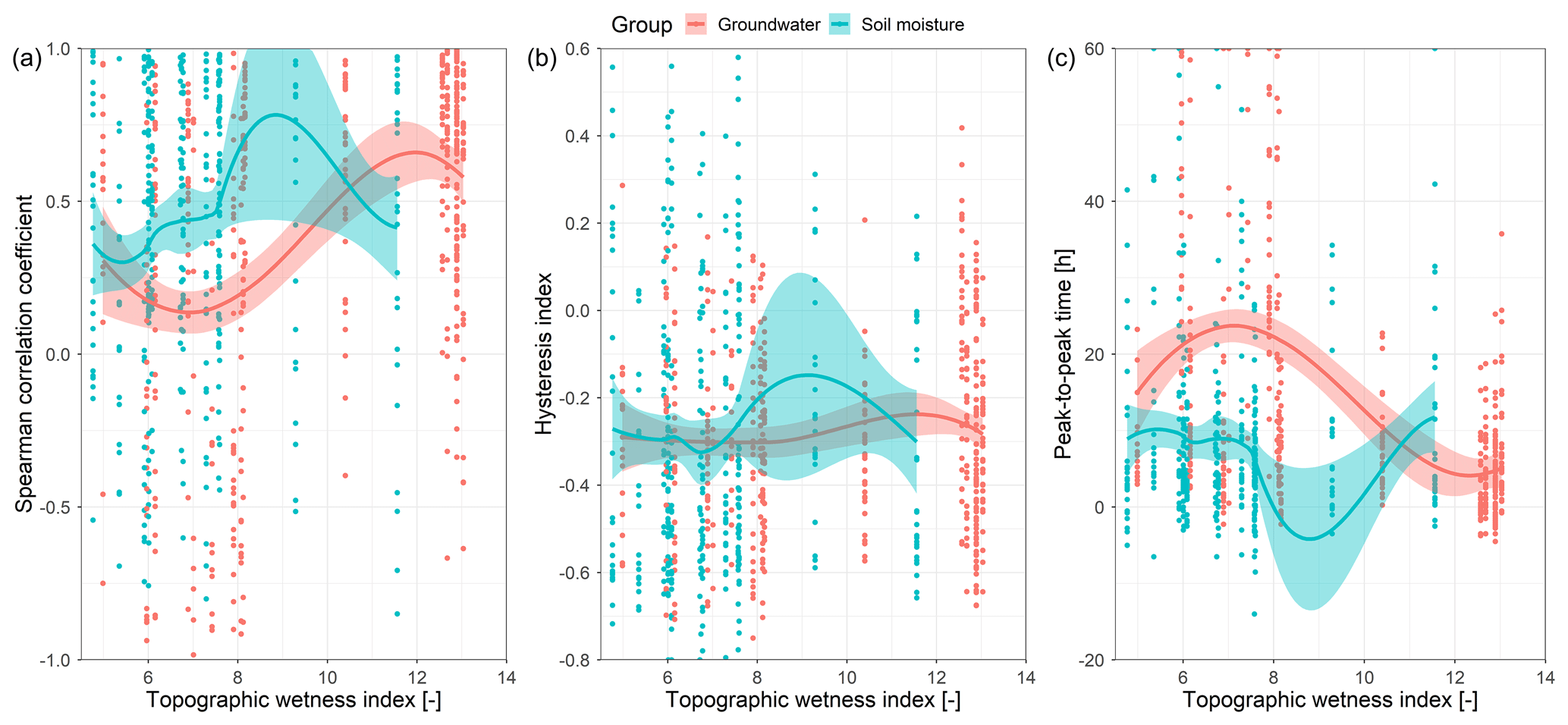
Figure A1 Spearman correlation coefficient (a), hysteresis index (b) and peak-to-peak time (c) of groundwater and soil moisture responses to streamflow event responses over locations with different topographic wetness indices. Colours represent different variable groups, i.e. groundwater and soil moisture. Points are calculated values for a single event and station; lines are local regression fits for each variable group and shaded areas the corresponding 95 % confidence intervals.

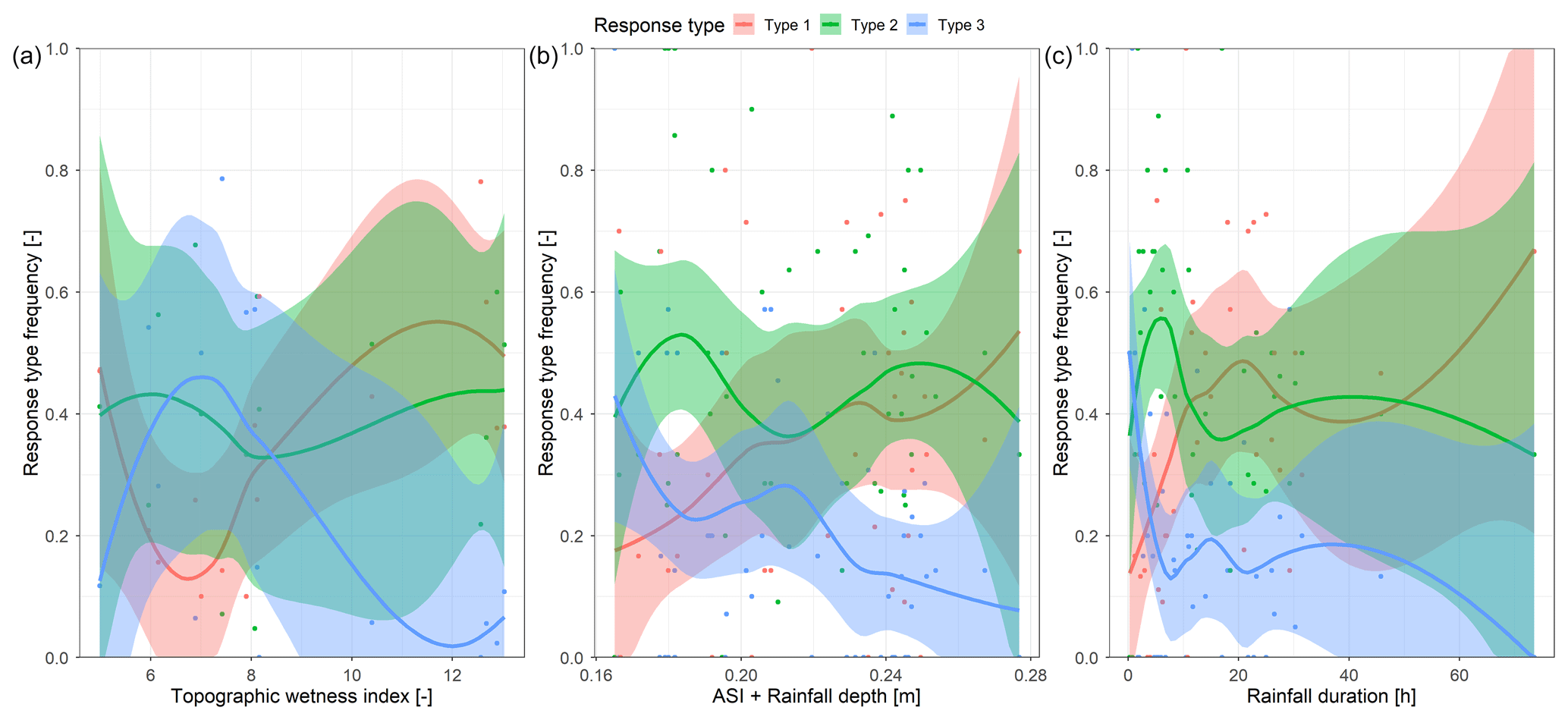
Figure A2 Groundwater response-type frequency over station topographic wetness index (a), a sum of antecedent wetness (ASI) and event rainfall depth (b) and rainfall event duration (c). Colours represent different response types as defined in Sect. 2.6. Points are calculated values of response-type frequencies; lines are local regression fits for each response type and the shaded areas corresponding to 95 % confidence intervals.

Figure A3 Soil moisture response-type frequency over station topographic wetness index (a), a sum of antecedent wetness (ASI) and event rainfall depth (b) and rainfall event duration (c). Colours represent different response types as defined in Sect. 2.6. Points are calculated values of response-type frequencies; lines are local regression fits for each response type and the shaded areas corresponding to 95 % confidence intervals.

Appendix B: Calculation of hysteresis index

Hysteresis index (HI) describes the size and rotational direction of a hysteresis loop. In this study, we use a calculation method similar to Zuecco et al. (2016). The calculation procedure is detailed below.

Let us have two time series x(t) and y(t) spanning the same period and with the same time steps, e.g. streamflow and groundwater responses to a precipitation event (Fig. B1a and b). First, the two time series are normalized:

$$\begin{array}{}\text{(B1)}& {\displaystyle }& {\displaystyle }u\left(t\right)={\displaystyle \frac{x\left(t\right)-x_{\min }}{x_{\max }-x_{\min }}},\text{(B2)}& {\displaystyle }& {\displaystyle }v\left(t\right)={\displaystyle \frac{y\left(t\right)-y_{\min }}{y_{\max }-y_{\min }}},\end{array}$$

where x_min, y_min, x_max and y_max are the minimum and maximum values in the time series x(t) and y(t), respectively; u(t) and v(t) are the normalized values of x(t) and y(t), respectively, which range between 0 and 1. We then plot v(t) against u(t) to obtain a hysteresis loop (Fig. B1c).

We then calculate the HI by integrating the curve of the hysteresis loop. We do this here by using the trapezoidal rule, i.e. summing up the trapezoidal areas under the curve (Fig. B1d):

$$\begin{array}{}\text{(B3)}& \mathrm{HI}=\sum _{k=\mathrm{1}}^N{\displaystyle \frac{v\left(t_k\right)+v\left(t_{k+\mathrm{1}}\right)}{\mathrm{2}}}\left(u\left(t_{k+\mathrm{1}}\right)-u\left(t_k\right)\right),\end{array}$$

where N is the number of time steps in the time series and v(t_k) and u(t_k) are the values of the normalized time series at the kth time step ($t_{N+\mathrm{1}}=t_{\mathrm{1}}$). Where the value of u(t) is increasing ($u\left(t_{k+\mathrm{1}}\right)-u\left(t_k\right)>\mathrm{0}$), the trapezoidal area has a positive contribution, and where u(t) is decreasing, the area has a negative contribution to the index. We get a value of HI between −1 and 1. The HI is positive for clockwise loops and negative for anticlockwise loops. It is close to zero when there is no hysteresis, for symmetrical figure-eight loops or some complex shapes. The magnitude corresponds to the loop's shape, i.e. the larger the loop, the closer the HI is to 1. The time step used is arbitrary and can even vary as long as it is the same for both time series and is fine enough to capture the observed processes. In contrast to the method of Zuecco et al. (2016), our method does not need the hysteresis loops to be split into rising and falling parts. This makes it applicable to any complex shape of the loop, for example, a two-peak rainfall-runoff event when streamflow rises and recedes two times. Nevertheless, results produced by our method are very comparable to the results of the method proposed by Zuecco et al. (2016).

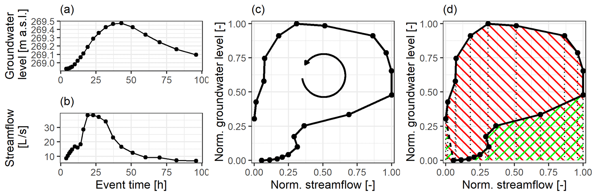
Figure B1 Example of the hysteresis index calculation: (a) and (b) show original groundwater and streamflow time series, respectively; (c) shows the anticlockwise hysteresis loop of the normalized time series from (a) and (b); (c) shows the positive and negative area contributions to the hysteresis index in a green and red pattern, respectively. Hysteresis index is −0.64.