Quantifying the effects of land use and model scale on water partitioning and water ages using tracer-aided ecohydrological models

Quantifying how vegetation mediates water partitioning at different spatial and temporal scales in complex, managed catchments is fundamental for long-term sustainable land and water management. Estimations from ecohydrological models conceptualising how vegetation regulates the interrelationships between evapotranspiration losses, catchment water storage dynamics, and recharge and runoff fluxes are needed to assess water availability for a range of ecosystem services and evaluate how these might change under increasing extreme events, such as droughts. Currently, the feedback mechanisms between water and mosaics of different vegetation and land cover are not well understood across spatial scales, and the effects of different scales on the skill of ecohydrological models needs to be clarified. We used the tracer-aided ecohydrological model EcH₂O-iso in an intensively monitored 66 km² mixed land use catchment in northeastern Germany to quantify water flux–storage–age interactions at four model grid resolutions (250, 500, 750, and 1000 m). This used a fusion of field (including precipitation, soil water, groundwater, and stream isotopes) and remote sensing data in the calibration. Multicriteria calibration across the catchment at each resolution revealed some differences in the estimation of fluxes, storages, and water ages. In general, model sensitivity decreased and uncertainty increased with coarser model resolutions. Larger grids were unable to replicate observed streamflow and distributed isotope dynamics in the way smaller pixels could. However, using isotope data in the calibration still helped constrain the estimation of fluxes, storage, and water ages at coarser resolutions. Despite using the same data and parameterisation for calibration at different grid resolutions, the modelled proportion of fluxes differed slightly at each resolution, with coarse models simulating higher evapotranspiration, lower relative transpiration, increased overland flow, and slower groundwater movement. Although the coarser resolutions also revealed higher uncertainty and lower overall model performance, the overall results were broadly similar. The study shows that tracers provide effective calibration constraints on larger resolution ecohydrological modelling and help us understand the influence of grid resolution on the simulation of vegetation–soil interactions. This is essential in interpreting associated uncertainty in estimating land use influence on large-scale “blue” (ground and surface water) and “green” (vegetation and evaporated water) fluxes, particularly for future environmental change.

1 Introduction

Climate projections indicate increases in temperatures and extreme drought frequency in many areas, with expected decreases in summer baseflow (Papadimitriou et al., 2016) and reduced summer soil water storage (Grillakis, 2019), which in turn limit evapotranspiration (Jung et al., 2010). Under climatic change, there are concerns that long-term partitioning of blue (groundwater and stream water) and green (evapotranspiration – ET) water fluxes may be adversely affected by land management for biomass production (i.e. agriculture and forestry; Falkenmark and Rockström, 2006). However, there is a limited evidence base to project the likely relative effects of climate and land use change on blue and green water fluxes (Orth and Destouni, 2018) and the associated predictive uncertainties (Mao et al., 2015). In regions susceptible to climatic extremes, there is a need to better quantify these fluxes to underpin sustainable long-term water and land use policies for anthropogenic (drinking water abstraction and irrigation) and natural (forest, wetland, and in-stream) ecosystem services. Ecohydrological modelling provides an approach to quantify blue and green water fluxes and associated storage dynamics and project future change. Ecohydrological models can bridge a gap between complex hydrological and ecological processes and capture their integrated effect in controlling water partitioning in the critical zone, i.e. the thin layer of the Earth encompassing the top of the vegetation canopy down to the bottom of the groundwater (Grant and Dietrich, 2017; Brewer et al., 2018). The feedback between ecology and hydrology is, however, strongly scale dependent, with controls on interactions vastly different across space and time (Fatichi et al., 2015). The interdependency of models on temporal and spatial scales often confounds identifiability of hydrological processes due to emergent behaviour, nonlinearity of parameter interactions, and aggregation effects at coarser resolutions when models are applied at larger scales (Wood et al., 1988; Blöschl and Sivapalan, 1995; Horritt and Bates, 2001; Samaniego et al., 2017). Many of the advancements in addressing difficulties in model scaling have focused on discharge (Samaniego et al., 2017) or soil moisture (Vereecken et al., 2008) due to limited alternative data and their information as proxies for large-scale water availability and atmospheric exchange. Nevertheless, the complexities of soil–vegetation interactions mandate further clarification of scaling effects and the resolution boundaries of fluxes across ecohydrological interfaces in the critical zone (Krause et al., 2017; Vereecken et al., 2019).

Water stable isotope tracers (deuterium and oxygen-18 and δ²H and δ¹⁸O, respectively) have been used as tools across various regions and spatio-temporal scales to improve estimates of ecohydrological partitioning (Bowen et al., 2011; Coenders-Gerrits et al., 2014; Tetzlaff et al., 2015; Jasechko, 2016). The integration of isotopic tracers in hydrological models is an effective way of constraining ecohydrological flux and storage dynamic estimates at both small (Ala-aho et al., 2017; Kuppel et al., 2018; Knighton et al., 2020) and large scales (Stadnyk and Holmes, 2020; Holmes et al., 2020). Integration of tracers into modelling frameworks also allows a nonstationary estimation of flux and storage water age dynamics for various critical zone compartments. As water age studies have historically focused on groundwater and stream water dating of blue fluxes, estimation of water ages in process-based, semi-distributed ecohydrological models to characterise the “hydro-demographics” of evaporation and transpiration is fundamental for a more comprehensive understanding of ecohydrological systems and their sensitivity to change (Kuppel et al., 2020). However, to date, such models have usually been applied in smaller, data-rich experimental catchments (<10 km²).

The main aim of this study was to explore changes in the skill of an ecohydrological model in capturing flux, storage, and mixing dynamics across spatial scales through application to a mesoscale (i.e. >10 km²) mixed land use catchment. We used the tracer-aided ecohydrological model EcH₂O-iso, which couples physically based hydrological conceptualisation with dynamic feedback mechanisms across the soil–plant–atmosphere continuum (Maneta and Silverman, 2013; Kuppel et al., 2018). EcH₂O-iso was developed with the intent of using diverse data in a multicriteria calibration and interfacing with large-scale climate models (Maneta and Silverman, 2013) through a fusion of field and remote sensing data. We seek to achieve the main aim of the study through the application of EcH₂O-iso in a drought-sensitive, agriculturally dominated catchment in northeastern Germany for an 11 year model simulation period, using four spatial resolutions. The study addresses three main research questions.

• Can a tracer-aided ecohydrological model effectively constrain estimates of water storage–flux–age interactions at different spatial resolutions in larger, mixed land use catchments?

• How are model uncertainty and parameter sensitivity affected by model resolution?

• Do specific data sets, for example, field (especially soil and stream isotopes) and remote sensing data (e.g. MODIS), aid in the identification of model resolution limitations for correct process representation?

The evaluation of these questions across different spatial model resolutions is aimed at providing a more robust understanding of the spatial boundaries of the ecohydrological exchange, partitioning, and uncertainty in models. This is a prerequisite for using such models in decision support to inform land and water management.

Table 1 Demnitzer Millcreek catchment climate data spatial and temporal resolutions from nearby weather stations, site collection, reanalysis data (short and longwave radiation; ERA5) and remote sensing data (leaf area index, latent heat, and ET; MODIS) used for daily modelling. Note: n/a – not applicable.

n/a stands for not applicable.

2 Study site and data

2.1 Climate and model forcing data

The 66 km² Demnitzer Millcreek catchment (DMC) is a catchment 55 km east of Berlin (52^∘23^′ N, 14^∘15^′ E), that receives 575 mm of precipitation annually. Cumulative annual precipitation varies from 372 to 776 mm yr⁻¹, with summer usually slightly wetter than winter due to convective storms, but winter is dominated by more frequent frontal rain (DWD, 2020). Potential evapotranspiration (PET) is very high relative to the annual precipitation (>600 mm yr⁻¹) and is generally only less than annual precipitation in very wet years (UFZ, 2020; Smith et al., 2020a). Long-term average air temperature and relative humidity are 10 ^∘C and 78 %, respectively (Smith et al., 2020a, b; Kleine et al., 2020).

A total of five long-term Deutscher Wetterdienst (DWD; German Meteorological Service) stations surrounding the catchment were used for long-term assessment (Table 1). As local measurements of incoming short- and longwave radiation were unavailable, these were derived from reanalysis data, ERA5 (ERA5; Hersbach et al., 2020). The ERA5 radiation is consistent with measurements near the DMC (Douinot et al., 2019) and has been successfully used for the estimation of ET, transpiration, and latent heat (LE; Smith et al., 2020b).

2.2 Soils and vegetation

The DMC land cover is dominated by non-irrigated arable crops in the northern headwaters and managed forests in the south; there is a long history of artificial drainage, especially in wetlands in the central catchment (Fig. 1a; Gelbrecht et al., 2005). The general land use is broadly representative of other extensive lowland agricultural areas in the North European Plain (e.g. Böse and Brande, 2010). The catchment is a long-term study site, with more than 30 years of monitoring agricultural pollution (Gelbrecht et al., 1996, 2005) and more recent detailed monitoring of stream isotopes, soil moisture, and soil isotopes (Smith et al., 2020a, b; Kleine et al., 2020).

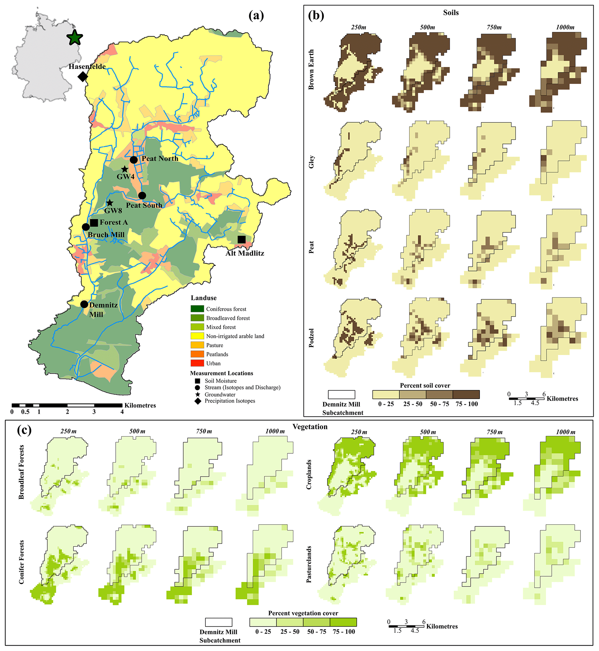
Figure 1 (a) The location of the Demnitzer Millcreek catchment (DMC) in Germany and field measurement locations within the DMC for soil moisture (squares), stream (circles), groundwater (stars), and precipitation isotopes (diamonds). (b) Soil coverage of brown earth, gley, peat, and podzol for spatial resolutions 250, 500, 750, and 1000 m. (c) Vegetation coverage of broadleaf forests, conifer forests, croplands, and pasture lands for each spatial resolution. Black boundaries show the calibration extent of the Demnitz Mill subcatchment.

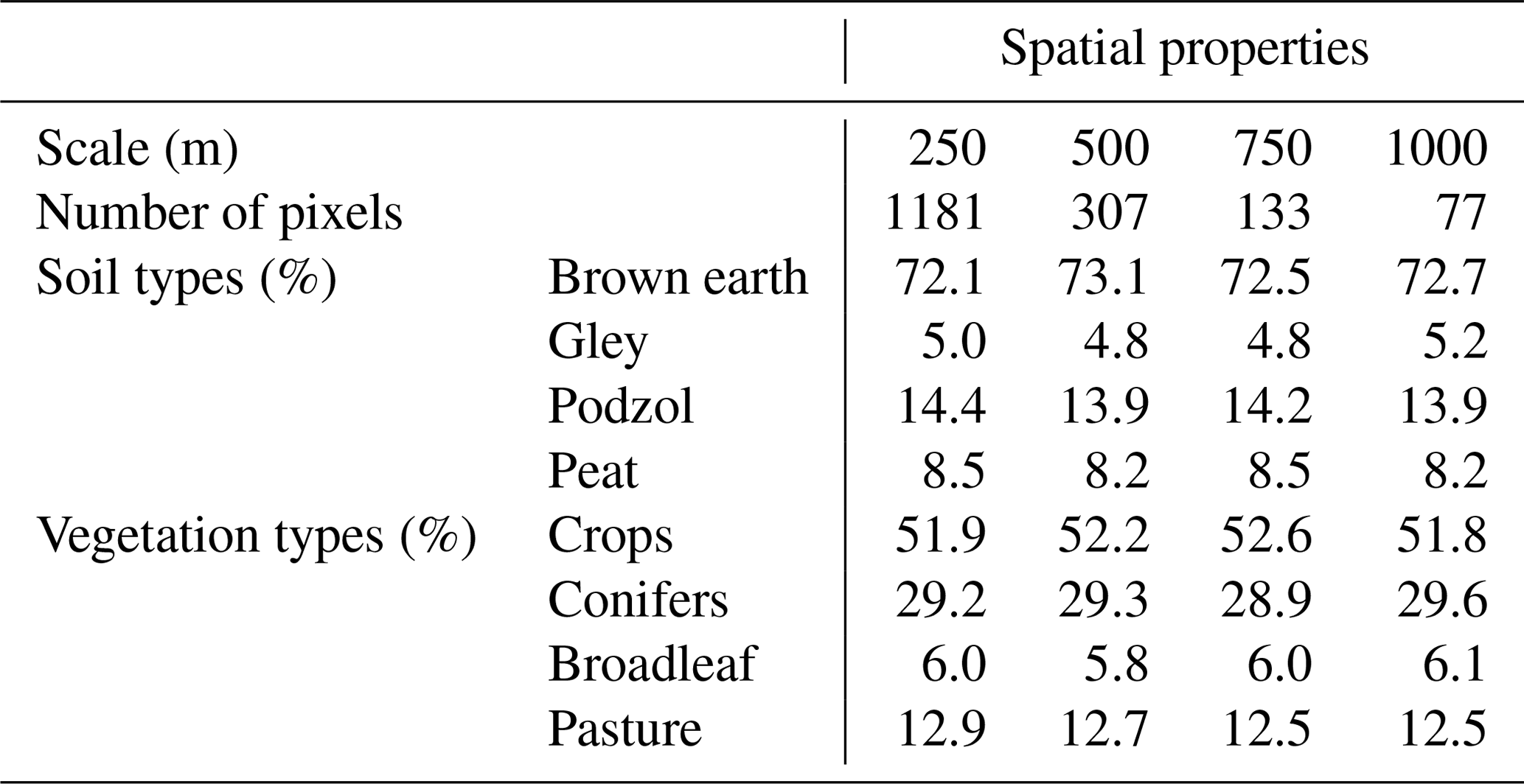
The catchment is characterised by four major soil types, with silty brown earths in the northern and southern regions, and sandy gleys, peats, and podzols dominating more central and southern regions (Fig. 1b). Brown earths are the most extensive soils (Fig. 1b; Table 2) and are siltier as a result of ground moraine deposited during the Pleistocene glaciation. Peats and sandy gley soils fringe the stream through the wetlands in the centre of the catchment and along the western edge of the catchment, respectively. The mid-catchment further from the stream is dominated by podzols and more sandy glacial deposits (Smith et al., 2020a).

Table 2 Catchment properties with percentages of soil type and vegetation type and the total number of pixels for different grid cell resolutions (at the Demnitzer Millcreek catchment outlet).

Vegetation is categorised into four major groups, i.e. croplands (arable), pasturelands, broadleaf forests, and conifer forests (Table 2; Fig. 1c). Croplands, primarily consisting of winter wheat, barley, and maize, occupy higher quality soils in the north (Kleine et al., 2020). Much of the pastureland is in peat fens that are poorly drained nutrient-rich soils unsuitable for crops and are therefore used for livestock grazing (Fig. 1c). Broadleaved forests are small and generally in the south, covering a limited area (Table 2). Conifer forests are the second most common cover, dominating the south and generally overlapping with the podzolic soils.

2.3 Hydrology of the Demnitzer Millcreek catchment

Discharge is measured at Demnitz Mill and the catchment outlet (Fig. 1 and Table 1). Streamflow is groundwater dominated, which results in a highly seasonal flow regime dependent on groundwater levels (Smith et al., 2020a). The catchment is situated on a large regional groundwater system that feeds the Spree River (Nützmann et al., 2014); however, regional groundwater–surface interactions only impact the catchment near the southerly outlet (Smith et al., 2020a). High-flow events primarily occur during the winter months due to more frequent low-intensity rainfall, lower ET, and wetter soils. Despite this, low runoff coefficients are common due to sandy soils limiting rapid lateral flow to only the most compacted or drained agricultural areas, saturated wetlands, and sealed surfaces (Smith et al., 2020a). The streamflow is very low during dry summer periods, with flow cessation having occurred more frequently and for longer durations since 2013 (Kleine et al., 2020). Dry summer periods are characterised by the relatively high ET, which limits annual groundwater recharge to winter months under forests (Smith et al., 2020b).

2.4 Isotopic data collection and analysis

Bulk water sample collection of precipitation and streams (Fig. 1a) was used for deuterium (²H) and oxygen-18 (¹⁸O) analysis. Daily bulk precipitation sampling began in mid-2018 with an autosampler (Fig. 1a). Stream isotope sample collection began at the beginning of 2018 as grab samples every second week at three locations (Peat North, Peat South, and Demnitz Mill; Fig. 1a). Daily stream sampling at Bruch Mill (Fig. 1a) began at the end of 2018, using an autosampler. Isotopic samples of stream water were only taken when streams were flowing and not during standing water. Evaporation was prevented by applying a layer of paraffin in all autosampler bottles. Bulk soil samples were collected monthly and soil water isotope composition was analysed using the direct-equilibrium method (analysis described in Kleine et al., 2020).

Bulk samples of precipitation, stream, and soil water were analysed in the IGB laboratory using a Picarro L2130-i cavity ring down water isotope analyser (Picarro, Inc., Santa Clara, CA, USA). Samples were standardised against the Vienna Standard Mean Ocean Water (VSMOW2) and are presented in δ notation.

A synthetic data set of isotopes in precipitation was created for the period prior to sampling (Table 1). This was based on the nearest local long-term δ²H monthly precipitation samples from Tempelhof in Berlin (Global Network of Isotopes in Precipitation – GNIP; IAEA/WMO, 2020). Monthly data were correlated against temperature and precipitation amounts, with the correlations used to randomly generate daily δ²H values (see Dehaspe et al., 2018). Random generations were repeated to minimise the difference between the synthetic amount-weighted δ²H values and the Tempelhof monthly δ²H data. The δ¹⁸O precipitation synthetic data set was developed using the predictive bounds of the local meteoric water line of the DMC to correlate δ²H to δ¹⁸O and generate variability.

3 EcH₂O-iso model set-up

The EcH₂O distributed ecohydrological model integrates modules for soil and vegetation to simulate energy and water balance, carbon uptake, and vegetation dynamics. The model is designed to be forced with inputs either from local climate stations or from regional climate models (Maneta and Silverman, 2013). EcH₂O was coupled with an isotope and water age module (EcH₂O-iso; Kuppel et al., 2018) to track δ²H and δ¹⁸O and estimate water ages in each model storage and flux. Here, we present an overview of the components of the water energy tracer flux– storage interactions that are relevant for the interpretation of results reported in this paper. A conceptual diagram of the storage and fluxes for energy and water balance is shown in Fig. S1 in the Supplement, with complete details of EcH₂O and EcH₂O-iso provided by Maneta and Silverman (2013) and Kuppel et al. (2018), respectively.

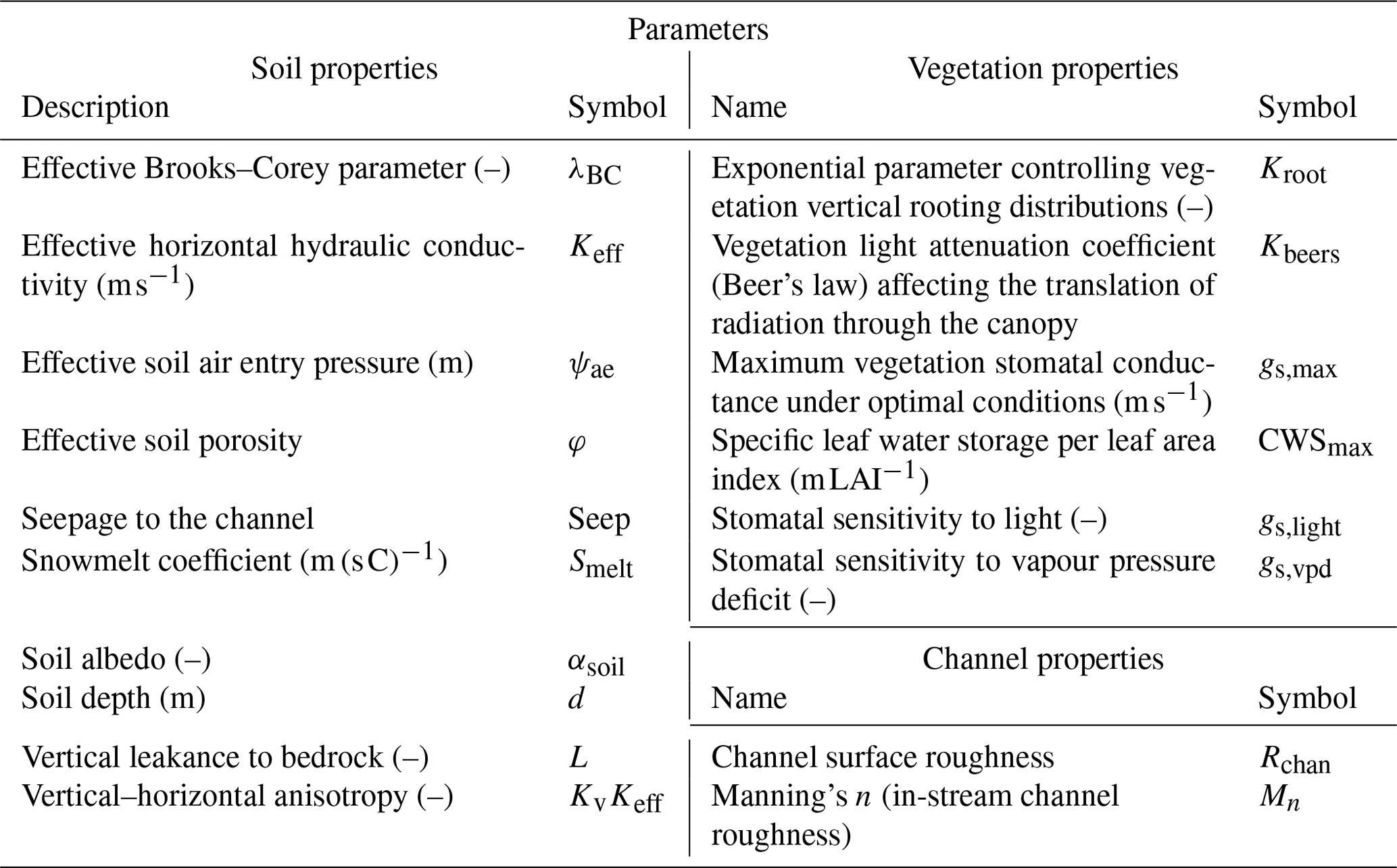
Table 3 Sensitive model parameters and descriptions for soil, vegetation, and channel properties. A full list of EcH₂O model parameters can be found in Maneta and Silverman (2013).

3.1 EcH₂O-iso energy balance

The energy balance of each model cell is solved for two layers (canopy and surface) and is driven by incoming shortwave and longwave radiation, as well as air temperature, relative humidity, and wind speed. The canopy energy balance resolves the effective canopy temperature that balances available radiative energy (net radiation), LE of interception and transpiration, and sensible heat exchanges. The model assumes that variations in canopy heat storage are negligible. The canopy energy balance is very sensitive to the availability of intercepted water (CWS_max; Table 3) for evaporation, the attenuation of radiation through the canopy (K_beer; Table 3), and the environmental constraints that limit transpiration, as implemented in a Jarvis-type stomatal conductance model (soil moisture, vapour pressure deficit, light, and temperature). The stomatal conductance model is dependent on the maximum physiological stomatal conductance of leaf water to the atmosphere (g_s,max; Table 3). Stomatal conductance is limited when vapour pressure deficit is high, with g_s,vpd (Table 3) controlling how sensitive the vegetation is to vapour deficit (low value decrease in stomatal sensitivity). Similarly, light conditions lower than optimal vegetation light requirements (g_s,light; Table 3) limit the stomatal conductance of the vegetation.

The surface energy balance resolves the surface temperature that balances surface net radiation with latent heat, sensible heat, snowpack heat, and ground heat exchanges. Unlike the balance for the canopy, energy storage variations in the snowpack and soil are important to accurately simulate snowmelt and effective soil temperatures and are taken into account in the solution of the surface energy balance. A new channel evaporation component was recently added and is solved using the same approach, i.e. estimating channel surface roughness (R_chan; Table 3) but neglecting heat storage components and ground flux exchanges.

3.2 EcH₂O-iso water balance

The water balance in EcH₂O-iso also uses a multilayered, top-down approach, with canopy, surface, and three subsurface (layers 1–3) storages (Fig. S1). Incoming precipitation is intercepted by vegetation. Interception amount, limited by leaf area index (LAI) and a specific leaf water storage parameter, controls the canopy water storage and throughfall. Throughfall and direct incident precipitation accumulates on the soil surface and infiltrates into soil layer 1 using the Green–Ampt model and Brooks–Corey parameter (λ_BC, Table 3) and air entry pressure (ψ_ae; Table 3; Te Chow, 1988). Infiltration excess is routed laterally as overland flow, as described below. Water infiltrated into the soil is vertically redistributed from the topsoil layer to lower layers, using a gravitational drainage model. Downward fluxes start when soil moisture exceeds field capacity at a rate driven by the vertical effective hydraulic conductivity (K_eff and K_vK_eff; Table 3), which increases linearly from zero at field capacity to saturated hydraulic conductivity when the layer is at saturation. Upward water redistribution can occur as storage excess when lower layers are fully saturated. Water can be extracted from the soil from the topsoil layer as evaporation, and as transpiration from any layer as a function of the proportions of roots contained in the layer. Water can also exit the soil profile as leakance to bedrock (or deeper groundwater) in layer 3 (L; Table 3). Return flow to the surface occurs when the entire soil profile is saturated and excess storage reaches the surface. Return flow is routed laterally as surface runoff.

Surface runoff, streamflow, and groundwater flow in the bottom-most soil layer are the lateral fluxes that are the three main mechanisms of later water redistribution. Water above field capacity in layer 3 of the soil is allowed to move laterally to the downstream cell, using a linear kinematic model driven by the cell slope. Surface runoff is generated from infiltration excess and return flows at the end of each time step. Overland flow is routed following a steepest descent approach until it reaches the channel and allows reinfiltration at every pixel along the flow path. The model assumes that overland flow generated at the end of the time step at any given pixel reaches the channel if it is not reinfiltrated along the flow path. Once water is in the channel, it is routed toward the outlet using a nonlinear kinematic wave model using a scaled Manning's n (M_n; Table 3) to attenuate channel water.

3.3 Water ages and isotope mixing and fractionation

The isotopic composition and water ages in channel storage and each subsurface store (layers 1, 2, and 3) are estimated using a complete mixing assumption (Kuppel et al., 2018) by which inflow is completely mixed with storage, using amount weighting of isotopes of inflow and storage. The inflow is the amount-weighted average of all inflow isotopes and ages to the storage. Outflow isotopic composition and water age from each storage (e.g. groundwater) are equal to that of the storage. Evaporative fractionation is estimated in soil layer 1 and open water using the Craig–Gordon fractionation model (Craig and Gordon, 1965). Fractionation of δ²H and δ¹⁸O in soils is conducted using the correction of relative humidity (Lee and Pielke, 1992), the kinetic fractionation factor (Mathieu and Bariac, 1996; Braud et al., 2005), and the Vogt (1976) kinematic diffusion value. Soil relative humidity is corrected with a sigmoidal function, based on the ratio of soil moisture to field capacity. The kinetic fractionation factor (n) is corrected using soil saturation to adjust the n value (liquid–vapour turbulence) between n=1 (dry soil) and n=0.5 (fully saturated soils; Mathieu and Bariac, 1996; Braud et al., 2005). Transpiration isotopes and water age were estimated as the amount-weighted average of root uptake from each soil layer (estimated via the energy balance). Open water (channel) fractionation is conducted with atmospheric relative humidity and open water kinetic fractionation factors. Given the decadal timescales of groundwater flow in the study region (see Massmann et al., 2009), we used mean residence time (MRT) estimations from groundwater volume (V) and flux (O; MRT $=V/O$) estimates in the model. The MRT formulation assumes continuous and equal mixing of water in storage, similar to the mixing processes invoked in the EcH₂O-iso water age module (Kuppel et al., 2018).

3.4 EcH₂O-iso model set-up and parameterisation

The model was set up at daily time steps for four resolutions, with squared cells of 250, 500, 750, and 1000 m. The model was run between 1 January 2007 and 31 December 2019, using the first 2 years as a spin up. To reduce the effect of the spatial resolution of climate model forcing data on model results (e.g. Liang et al., 2004), forcing data were included as representative polygon areas from five local climate stations (Table 1). The area of each zone was defined using the distance of the climate station and the Thiessen polygon method. Isotopes in precipitation were applied uniformly across the catchment, as limited spatial differences in isotopic compositions were observed. Averaged 8 d LAI values were used to improve the estimation of the interception capacity through all seasons. Spatial and temporal patterns of LAI were determined using MODIS data (Table 1), with the upper limit of the croplands and pasturelands corrected using ground measurements and other nearby studies (Wegehenkel et al., 2017; Drastig et al., 2019). Soil and vegetation maps were initialised for the highest (250 m) cell resolution, consolidating soil and vegetation percentages with increasing cell size to keep the same proportion of soil to vegetation for each resolution. Soil parameters for each cell were weight averaged, using the proportion of each soil type (brown earth, podzol, peat, and gley; Fig. 1b). A proportion-weighted geometric mean was used for soil conductivity and anisotropy (Sanchez-Vila et al., 2006; Bizhanimanzar et al., 2020). The soil water leakance parameter was nonzero to modulate interactions between the deeper regional groundwater system (not modelled) and the shallower groundwater system (modelled). Soil, stream, and groundwater isotopic compositions were initialised using soil, stream, and groundwater measurements in 2018 and 2019.

3.5 Model evaluation, calibration, and validation

3.5.1 Evaluation

The model was evaluated using two efficiency criteria, namely the Nash–Sutcliffe efficiency (NSE; Nash and Sutcliffe, 1970) and the normalised mean absolute error (NMAE). Discharge and soil moisture in layer 1 were evaluated at two locations (Fig. 1a) and ET and LE at three locations, using NSE. The first soil moisture site was evaluated at forest site A (herein referred to as forest A), which is typical of a managed mixed forest over podzolic soils in the DMC (Smith et al., 2020b; Kleine et al., 2020). The second soil moisture site was evaluated at Alt Madlitz (herein referred to as cropland), which has similar soil (brown earth) and vegetation (croplands) to the northern reaches of the catchment. A fusion of measured soil moisture and estimated soil moisture for the ERA5 reanalysis data sets were used to calibrate soil moisture at each site. All stream isotope (four locations), soil isotope (one location), groundwater isotope (two locations), and transpiration (one location) simulations were evaluated using the NMAE. NMAE was used due to inconsistent time steps of data collection, while emphasising data set variability without the higher weighting of peak values typical of the NSE.

Correlations between fluxes, storages, water ages, and the proportion of vegetation and soils (i.e. spatial proportions in Fig. 1b and c) were assessed using the Spearman's rank correlation (Sect. S5). The Spearman's rank correlation was used as it does not assume a normal distribution. The significance of the correlations was assessed to 95 % confidence.

3.5.2 Sensitivity analysis

Sensitivity analysis in the DMC was conducted for each model resolution, using a modification of the Morris method (Morris, 1991; Sohier et al., 2014). This is a step-wise sensitivity test, changing model parameters one at a time and quantifying the resulting magnitude of change in model output. Parameter sensitivity was assessed, using 75 trajectories with randomised initial parameters (Latin hypercube sampling – LHS; McKay et al., 1979), to establish a synthetic baseline. Radial sampling was utilised in a step-wise manner, varying each parameter by 50 % of the range. All possible model parameters were included to identify the most sensitive parameters for use in calibration. Output time series (ET, LE, discharge, and soil moisture) were evaluated against the synthetic baseline using the root mean square error (RMSE). The RMSE of output for each trajectory was averaged to give an overall parameter sensitivity.

3.5.3 Calibration

Using the most sensitive parameters identified by the analysis, 100 000 parameter sets were generated for Monte Carlo simulations, using LHS to optimise sampling space. As the parameter ranges were set to be the same for all spatial resolutions, the same parameter sets (100 000) were used. Calibration was conducted by multicriteria calibration, using fluxes, discharge, and isotopes (Table 1). Model testing revealed that 2 years of spin up (January 2007–December 2008) were sufficient to initialise the soil moisture storage, groundwater, and discharge. Initial conditions for water ages in storages were determined using previous estimates of shallow soil water (Smith et al., 2020b) and nearby tritium groundwater age estimates (Massmann et al., 2009). Regression of water age time series was conducted (p value <0.05) to ensure that no significant long-term change in water ages was present. Model calibration was conducted with a discontinuous period, 2009–2014 and 2018–2019, with the 2015–2017 years used for validation. The calibration period was selected due to a combination of high- and low-flow extreme events and data availability. The calibration extent was limited to the Demnitz Mill subcatchment (Fig. 1b and c) due to the strong regional groundwater interaction with surface water at the outlet of the DMC (Smith et al., 2020a). Multicriteria calibration (Sect. 3.5.1) was conducted using normalised efficiency criteria in empirical cumulative distribution functions (eCDF) to rank the best overall efficiency (Ala-aho et al., 2017; Smith et al., 2020c). Due to the large discrepancies in the number of samples of calibration data (e.g. 8 d data for the whole time-period vs. weekly stream isotope data for 2 years), the empirical cumulative distributions (eCDF) were inversely weighted by the number of samples (e.g. additional weighting was given to isotopic simulations relative to discharge). A threshold quantile for the weighted eCDF was determined for each model resolution to produce exactly 100 parameter sets (Ala-aho et al., 2017). Posterior parameter ranges of calibrated parameters are provided in Table S2 and Fig. S3. Single calibration was conducted for each model output to directly compare the effect of multicriteria calibration on model output trade-off. The significance of the difference in efficiency criteria at each resolution was assessed using the Wilcoxon rank sum test (Mann and Whitney, 1947). The Wilcoxon rank sum test does not assume a distribution and is, therefore, more robust in the comparison of efficiency criteria.

3.5.4 Validation

Model validation was conducted for the years not used for calibration (2015–2017). The validation years had average flow conditions relative to the long-term measurement and were, therefore, representative of the average conditions of the catchment. The model was validated against measured discharge at Demnitz Mill, remotely sensed ET and LE, and soil moisture estimated from ERA5 reanalysis products at the same sites as calibration (Table S3). Since isotopic measurements (stream, soil, and groundwater) began in 2018, isotopic data were not available for validation. “Soft” validation was assessed, using soil isotopes not used in calibration (soil layer 2 and cropland isotopes layer 1) in 2018–2019.

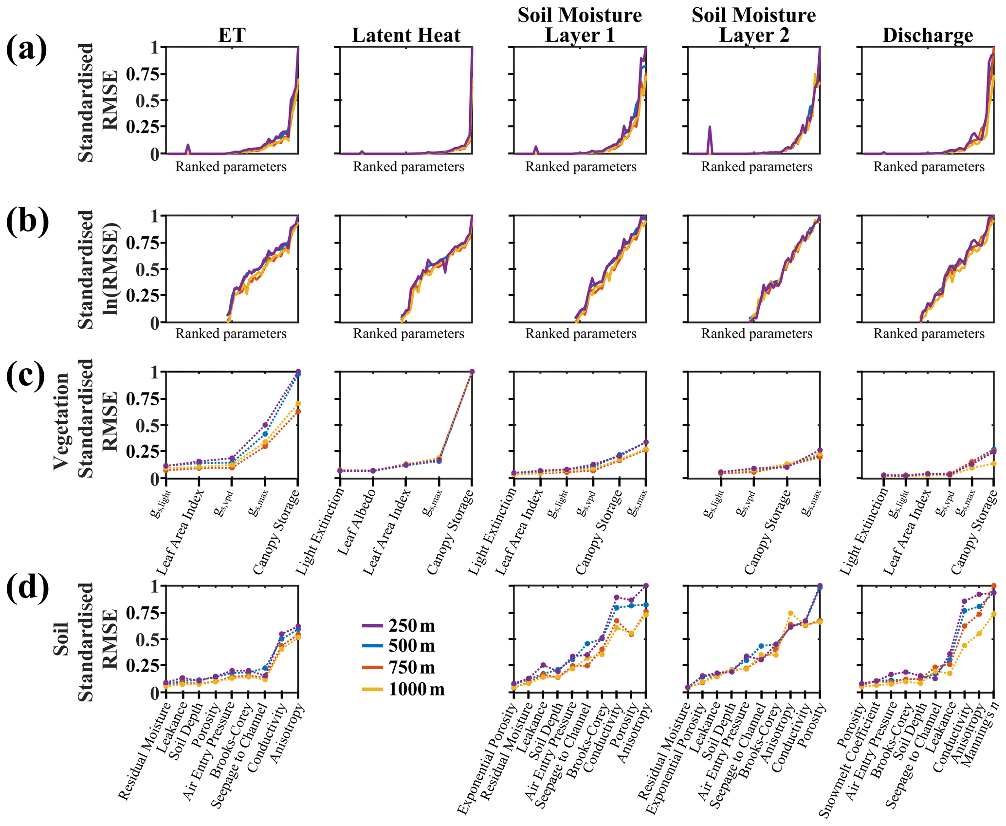
Figure 2 (a) Standardised root mean square error, (b) standardised root mean square error for the most sensitive vegetation parameters, and (c) standardised root mean square error for the most sensitive soil parameters for each output and spatial resolution. Vegetation parameters, g_s, are the control of vegetation stomatal conductance, with maximum potential conductance (g_s,max), light-controlling conductance (g_s,light), and vapour-pressure-deficit-controlling conductance (g_s,vpd).

4 Results

4.1 Sensitivity to model spatial resolution

The ranked sensitivity of model output (standardised RMSE between 0 and 1 for maximum and minimum of all resolutions) against all model parameters (18, 30, and 6 parameters for each soil, vegetation, and channel, respectively) showed that the RMSE of model output is sensitive to a few parameters which control the dominant fluxes (Fig. 2a). This resulted in the selection of a much smaller number of calibrated parameters (Sect S2; 10, 6, and 4 parameters for each soil, vegetation, and channel, respectively). Regardless of the calibration against remote sensing products (ET and LE), field data (discharge), or fusion of data sources (soil moisture), results showed high nonlinearity against the ranked parameters (low average sensitivity to high average sensitivity). Each grid resolution showed a similar nonlinearity of RMSE to parameters. Splitting the ranked parameters into the vegetation and soil parameters isolated their contribution to the sensitivity of each output (Fig. 2b and c). The standardised RMSE showed higher sensitivity of parameters for all outputs when the resolution was finer (Fig. 2b and c). Specifically, greater separation of sensitivity was present in the vegetation parameters mainly influencing ET (Fig. 2b) and soil parameters regulating soil moisture and discharge (Fig. 2c), with the largest change with resolution occurring between 500 to 750 m. Latent heat and soil moisture in layer 2 did not show differences in parameter sensitivity between resolutions for either vegetation or soil parameters, underlining the importance of layer 1 in water partitioning.

The output for calibration to remote sensing products (ET and LE) was most sensitive to vegetation parameters (Fig. 2b), particularly canopy water storage (CWS_max) and maximum stomatal conductance (g_s,max). Large parameter ranges in CWS_max resulted in high variation in LE and, thereby, ET and interception evaporation (not shown). At all resolutions, stream discharge was sensitive to three parameters, namely Manning's n (M_n), horizontal saturated hydraulic conductivity (K_eff), and vertical to horizontal hydraulic conductivity anisotropy (K_vK_eff).

Table 4 Median model efficiency from multicriteria calibration (the brackets indicate the efficiency criteria).

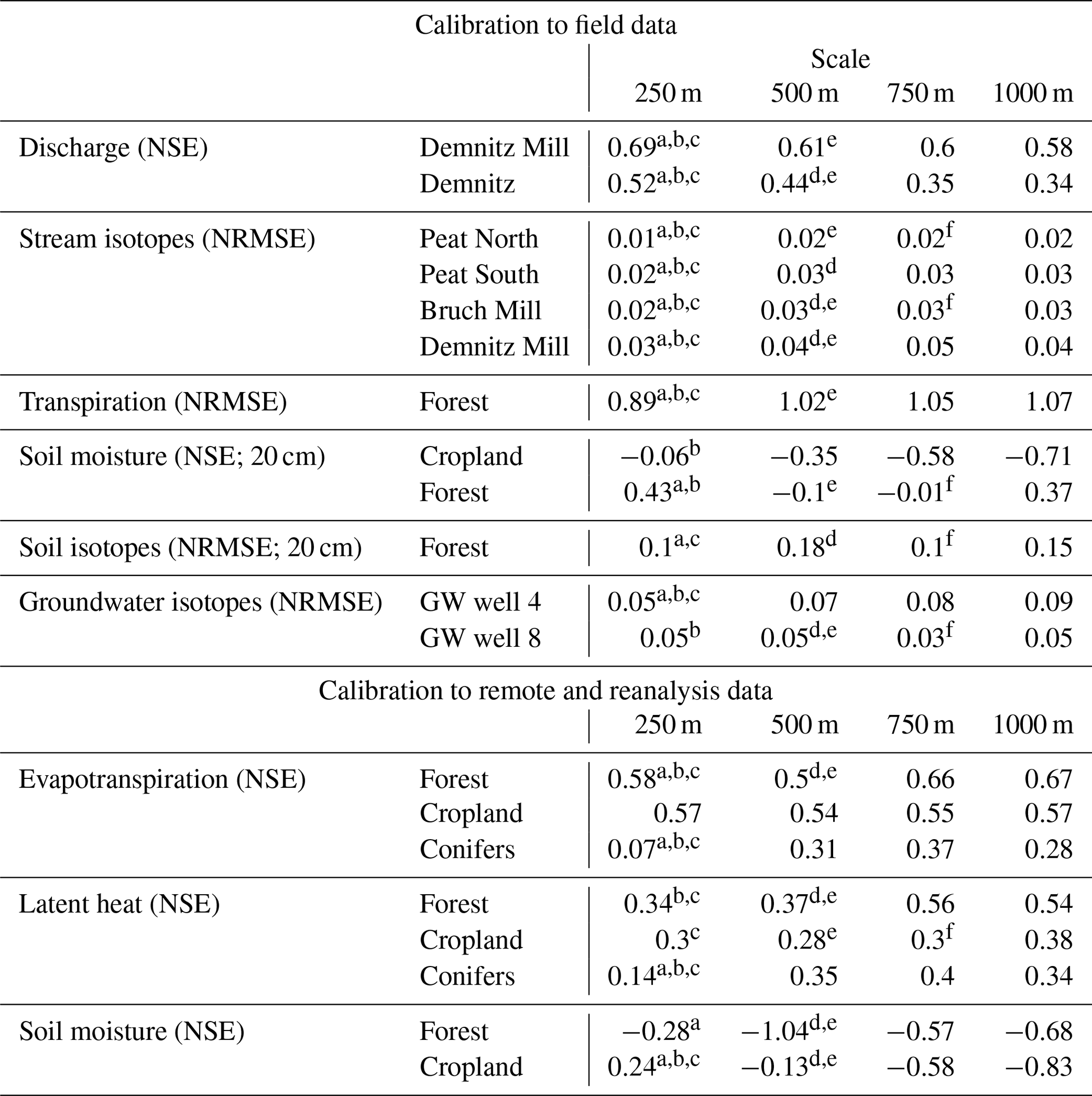
Superscripts indicate a significant difference of efficiency between model scales, where ^a is 250 vs. 500 m, ^b is 250 vs. 750 m, ^c is 250 vs. 1000 m, ^d is 500 vs. 750 m, ^e is 500 vs. 1000 m, and ^f is 750 vs. 1000 m.

4.2 Effects of model resolution on calibration

The values of the median calibration efficiency criteria of the 100 “best” parameter sets for each model output and resolution suggest that dominant catchment processes were reasonably captured (Table 4). Median validation efficiencies generally showed small decreases compared to the calibration period (Table S3). Multicriteria calibration showed different trade-offs in efficiency between resolutions (Table 4) with the maximum model efficiency (i.e. single model calibration; Table S1 ) not simultaneously met. Except for ET and LE (calibration to remote sensing data), the model performance was substantially better at finer resolutions (Tables 4 and S1). While simulations of soil moisture displayed a relatively high single calibration efficiency (Table S1), multicriteria calibration resulted in lower model performance (Table 4).

Field data had the greatest benefit for constraining results at finer resolutions, most notably with significant improvements in discharge and stream isotopes (Table 4). Additionally, transpiration dynamics (in the mixed forest) were greatly improved at 250 m, relative to the other resolutions, despite similar vegetation percentages at the location for all resolutions (Fig. 1c). Similarly, a greater capability for simulating soil moisture was apparent at finer resolutions. However, significant improvements in soil moisture with decreasing resolution were not consistent.

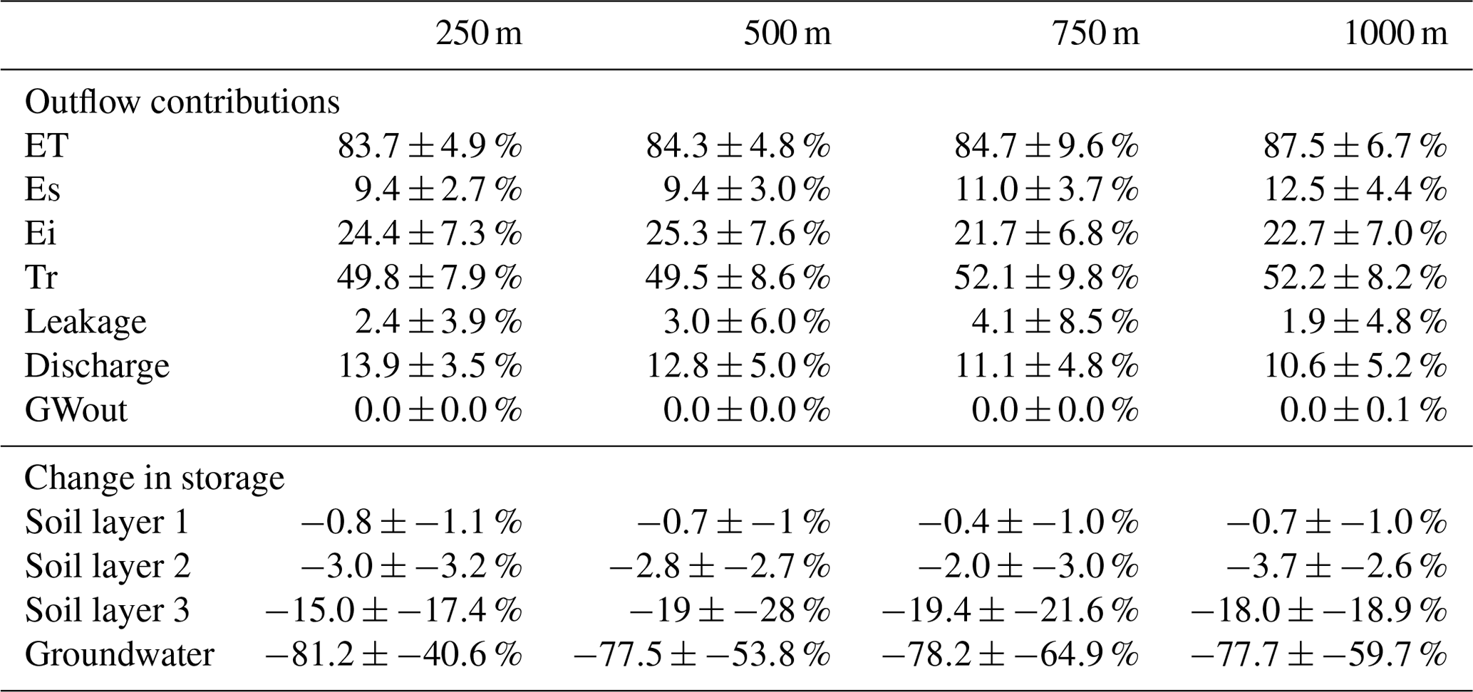
Model output calibrated against remote sensing data also showed mixed patterns of model performance between resolutions (Table 4). In general, coarser resolutions performed better against remote sensing data than finer resolutions through both single calibration (Table S1) and multicriteria calibration (Table 4). The modelled water balance fluxes were quite similar across scales (Table 5). The largest contribution of precipitation loss within the catchment was ET, accounting for >80 % of total precipitation. Transpiration was the dominant component of ET, accounting for ∼50 % of losses, with interception evaporation (Ei – 21 %–25 %) and soil evaporation (Es – 9 %–12 %) much smaller. Secondary outflows of the catchment were stream discharge (11 %–14 %) and vertical groundwater leakance (2 %–4 %) to the deeper regional aquifer (Table 5).

Table 5 Mean catchment outflow contribution over the simulation period (2009–2019), as a proportion of the total catchment outflow, and the percent change of catchment storage from the beginning of 2009 to the end of 2019. Contributions include evapotranspiration (ET), soil evaporation (Es), interception evaporation (Ei), transpiration (Tr), leakage, discharge, and groundwater outflow (GWout). Standard deviations of the contributions and storage changes are derived from the 100 best simulations for each resolution.

4.3 Resolution effects on estimations of discharge and stream isotopes

All model resolutions were able to adequately simulate discharge at both Demnitz and Demnitz Mill, with minor improvements in low flows at coarser resolutions and improvements in high flows at finer resolutions (Fig. 3a and b). Uncertainty was also lower with finer grids. Isotopic simulations in the northern reaches of the catchment were constant and relatively similar between resolutions (Fig. 3c). More notable deviations of median simulations between resolutions were evident at stream sites downstream of the wetland between Peat North and Peat South (Figs. 1a and 3b–d); with a failure to reproduce winter depletion and summer-enriched isotopes at resolutions >500 m. While enrichment of in-stream isotopes could be reproduced for a single calibration at coarser resolutions (Table S1), multicriteria calibration was unable to capture isotopic enrichment simultaneously at all downstream sites. Multicriteria calibration resulted in a wide range of simulated in-stream isotopic compositions at coarser resolutions (750 and 1000 m; Fig. 3c–f), consistent with simulations of spatially extensive overland flow events that are not present at finer resolutions. The range of upper and lower bounds of simulated stream isotopes increased notably between Peat North and Peat South, as a result of both the uncertainty of process representation and wetland open water fractionation within the wetlands (Fig. 3c and d). These uncertainties were primarily within the wetlands, with the range of upper and lower bounds decreasing with distance from Peat South (Fig. 3e and f). For all stream isotope locations, the range of upper and lower bounds decreased with coarser model resolution.

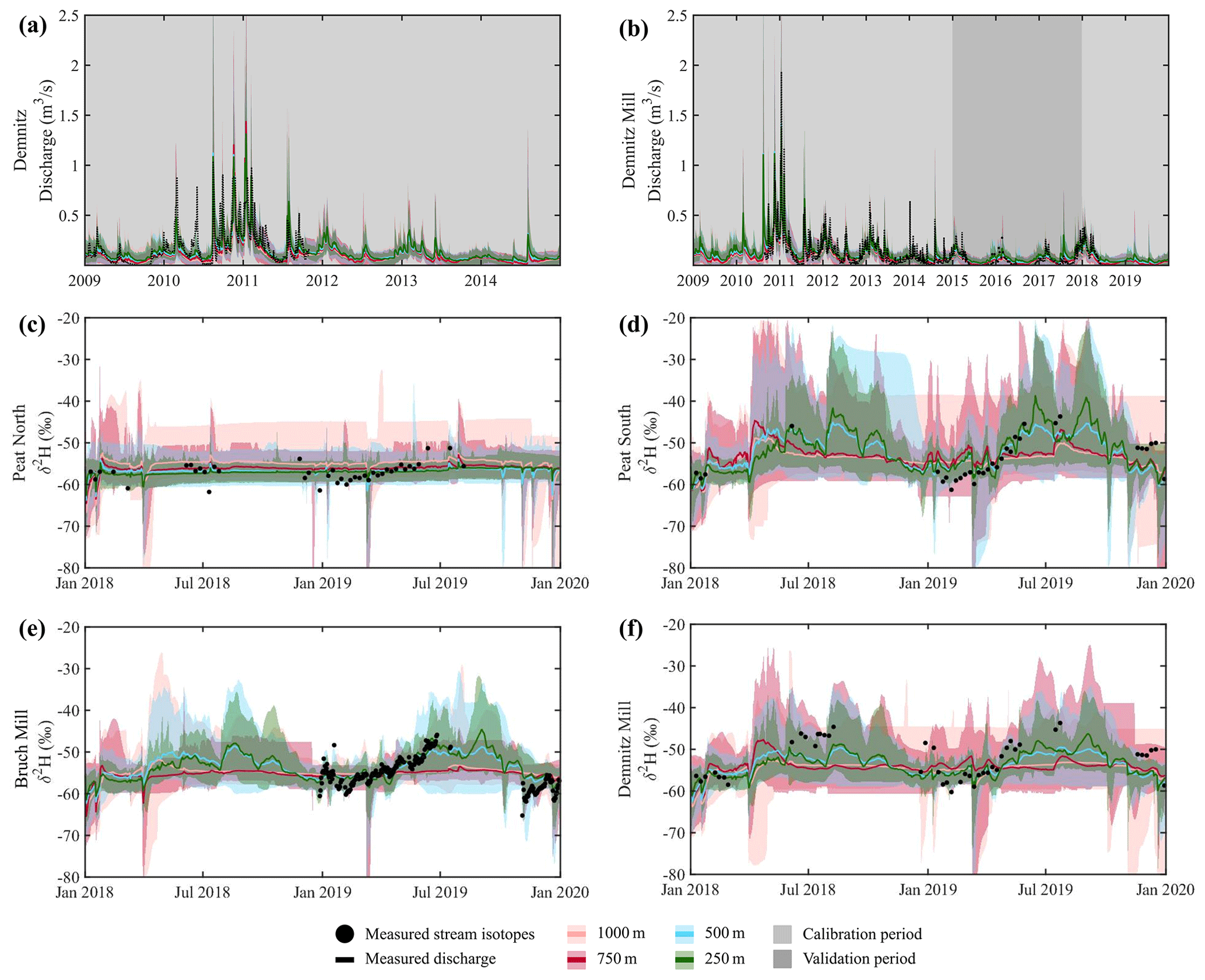
Figure 3 Simulated discharge at (a) Demnitz and (b) Demnitz Mill and stream isotopes at (c) Peat North, (d) Peat South, (e) Bruch Mill, and (f) Demnitz Mill. Colours indicate the model resolution, with the solid lines showing the median simulation and the shaded regions showing the upper and lower simulation bounds.

4.4 Effect of model scale on ecohydrological fluxes and storages

Calibration of ET and transpiration used a data fusion of remote sensing ET (MODIS) and field measurements of sap flow at forest A. Calibration of ET to the 8 d MODIS ET showed a small (19 mm) increase in the median annual catchment ET estimated by coarser resolutions (Fig. 4a–d) but with increased uncertainty. This difference between resolutions was small in comparison to the uncertainty of annual ET. Spatially, ET had a positive correlation with coniferous forest cover and peaty and podzolic soil cover at most resolutions and a consistent negative relationship to the proportion of pastureland and brown earth soils (spatial comparison of Figs. 1 and 4; statistical correlations shown in Fig. S5). The fraction of transpiration to ET (Fig. 4e–h) was also relatively consistent between resolutions, with only a slight decrease at coarser scales. The uncertainty of the ratio of transpiration to ET did not notably change between resolutions (Fig. 4; Table 5). Unlike ET, transpiration had strong dependencies on both vegetation and soil proportions at all resolutions (Figs. 1, 4, and S5). Specifically, transpiration strongly increased with higher proportions of croplands and brown earth and strongly decreased with higher proportions of conifer and pasturelands and peaty and podzolic soils. Like ET, the ratio of Es to ET increased moderately with the model resolution, but the increase was still within the model uncertainty. Es showed a much weaker dependency on soil or vegetation proportion, with only higher proportions of pastureland and peaty soil significantly increasing Es. Median annual channel evaporation was relatively constant, from 250 to 750 m resolutions, with a slight decrease from the 750 m resolution to the 1000 m resolution (Fig. 4m–p). Channel evaporation periodically resulted in dry channels and a discontinuous channel network during dry periods (not shown), which was consistent with stream connectivity observations in the field. The annual ratio of recharge to ET, and the ratio uncertainty, was consistent across all resolutions (Fig. 4q–t). Spatially, recharge was closely linked to soil cover, with a moderately positive correlation with brown earth and moderately negative correlations with peaty and podzolic soils. However, the proportions of conifers showed the strongest links with annual recharge, which greatly decreased with higher proportions of conifers. The decrease in annual recharge is largely linked to the higher ET (Figs. 1, 4, and S5).

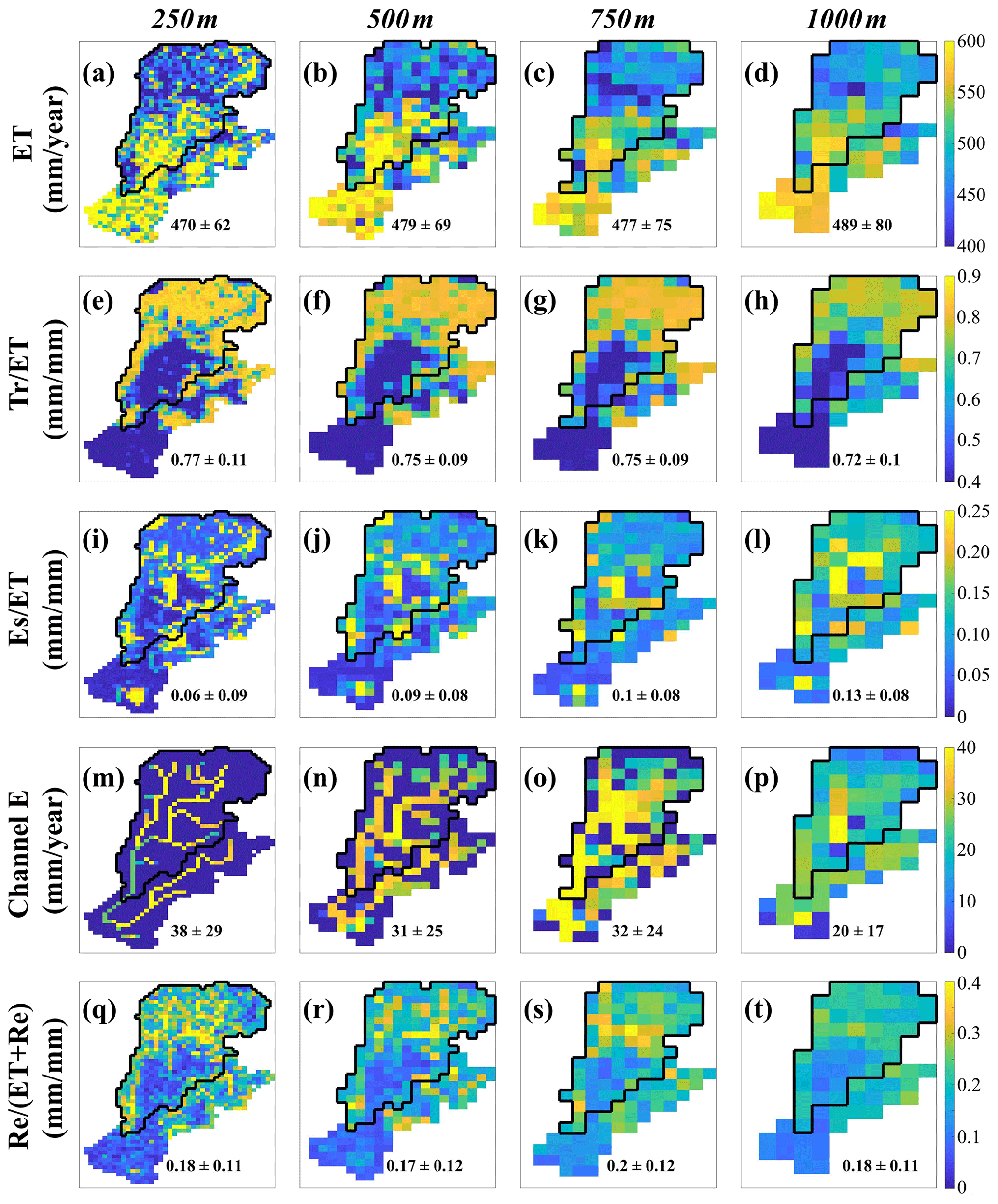
Figure 4 The (a–d) average annual evapotranspiration (ET), (e–h) ratio of transpiration (Tr) to ET, (i–l) ratio of soil evaporation (Es) to ET, (m–p) channel evaporation (channel E), and (q–t) the recharge proportion of vertical flux (recharge and ET) for the 250, 500, 750, and 1000 m resolutions. Black boundaries show the calibration extent of the Demnitz Mill subcatchment. Values shown are the catchment-wide, long-term (2009–2019) average values and average standard deviation (average of each pixel) within the Demnitz Mill subcatchment.

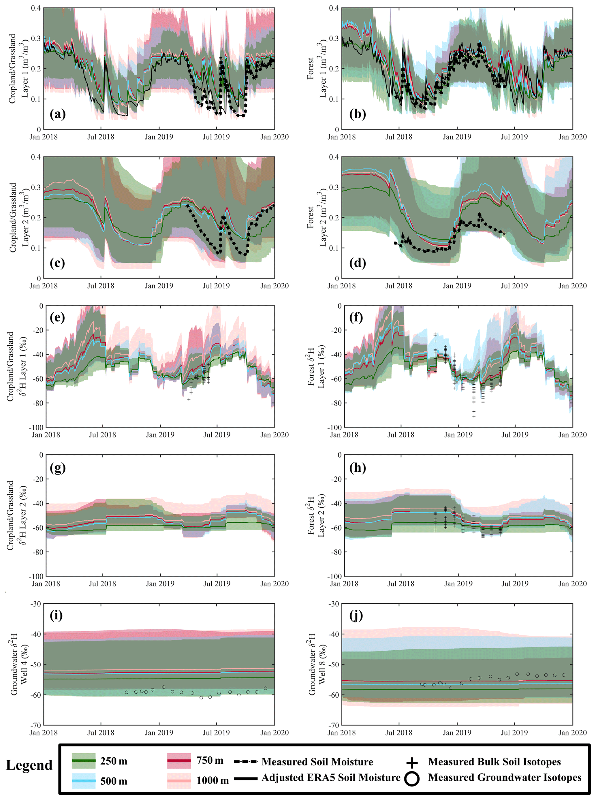
Figure 5 Simulations and measured soil moisture in layers 1 (a, b) and layer 2 (c, d) in the croplands (a, c) and in the forest (b, d). Also shown are adjusted ERA5 soil moisture estimates at the same locations. Measured and simulated soil isotopes in layer 1 in (d) the forest (e) the cropland, and layer 2 in (g) the forest and (h) the cropland. Simulated and measured groundwater isotopes at (i) groundwater well 4 (GW 4) and (j) groundwater well 8 (GW 8).

Calibration of soil moisture in layer 1 (against measured data and ERA5 reanalysis) in the cropland and forest sites provided adequate representation of the measured dynamics (Fig. 5a and b, respectively). All model resolutions showed slight over-wetting of the soils in both layers 1 and 2 during the summer months (June–August; Fig. 5a–d), with simulations closer to ERA5 reanalysis than measured soil moisture. Except for the 500 m grid, the range of the upper and lower bound in soil moisture decreased with a coarser model resolution. The dynamics of simulated soil isotopes in the forest (calibrated) and grassland (validated) captured measurements at all resolutions and depths, with a slight increase in enrichment with increasing resolution (Fig. 5e–h). The ranges in the upper and lower simulation bounds were notably smaller in the 250 m resolution during periods of measurement; however, the ranges in the simulation bounds were more similar when calibration data were not available. The model adequately reproduced the relatively stable field measurements of groundwater isotopes in wells 4 and 8, with limited differences in either the median or simulation bounds between resolutions (Fig. 5i and j).

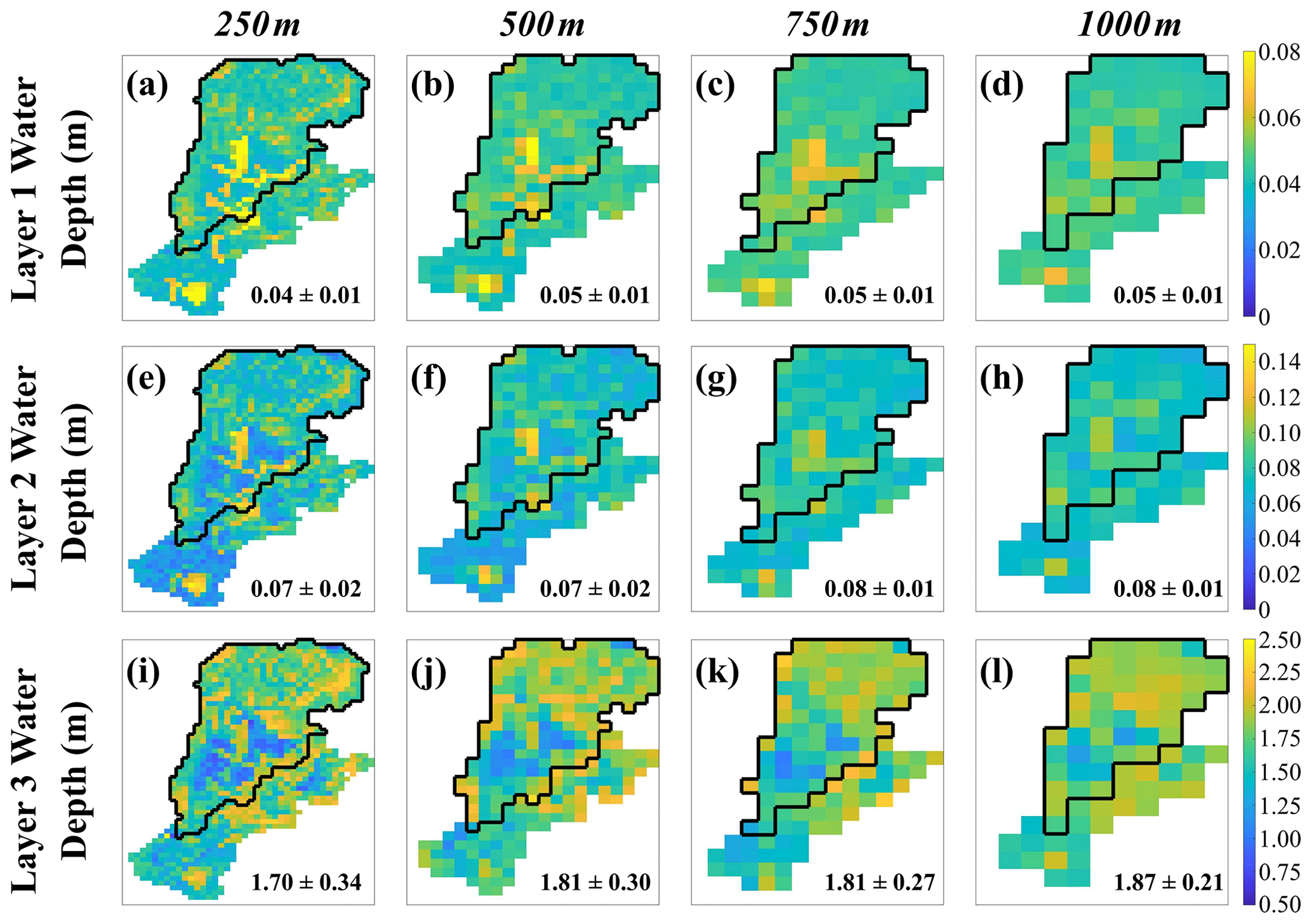
Figure 6 The (a–d) median annual equivalent water depth in layer 1, (e–h) median annual equivalent water depth in layer 2, and (i–l) median annual equivalent water depth in layer 3 for the 250, 500, 750, and 1000 m resolutions. Black boundaries show the calibration extent of the Demnitz Mill subcatchment. Values shown are the catchment-wide, long-term (2009–2019) median values and average standard deviation (average of pixel standard deviation) within the Demnitz Mill subcatchment.

Annual median equivalent soil water depths in layers 1–3 were relatively consistent for each model resolution (Fig. 6). The uncertainty of equivalent water depth in layers 1 and 2 was small relative to layer 3, due to non-calibrated soil depths in the first two soil layers (Sect. S2). Higher proportions of pastureland and peaty soil strongly increased modelled soil storage in layers 1 and 2 and, consequently, greatly increased soil evaporation (Figs. 1, 6, and S5). There was a weak negative relationship between soil storage and croplands, with a strong negative relationship with conifers; however, the dependency of soil storage on conifers was not consistent for all model resolutions. Layer 3 storage had much stronger (negative) correlations with both vegetation (conifers) and soils (brown earth and podzolic soils) for all resolutions than the upper soil layers. Notably, all storages decreased over the time of the simulations (2009–2019), mainly as a result of the 2018–2019 drought (Table 5).

4.5 Ages of ecohydrological fluxes

There was a notably older estimated shallow soil water age (layers 1 and 2) at the 250 m model resolution relative to all coarser model resolutions (shown for summer months in Fig. 7a–h; seasonal ages in Table S4). Uncertainty of water age estimates in each layer also generally decreased with coarser resolutions as these were trivial in layer 1 but more notable in layer 2. Water ages in layers 1 and 2 strongly decreased with increased transpiration and recharge and higher proportions of croplands and brown earth. Conversely, water ages (layers 1 and 2) strongly increased with higher proportions of conifers and peaty and podzolic soils for all model resolutions (Figs. 1, 7, and S5).

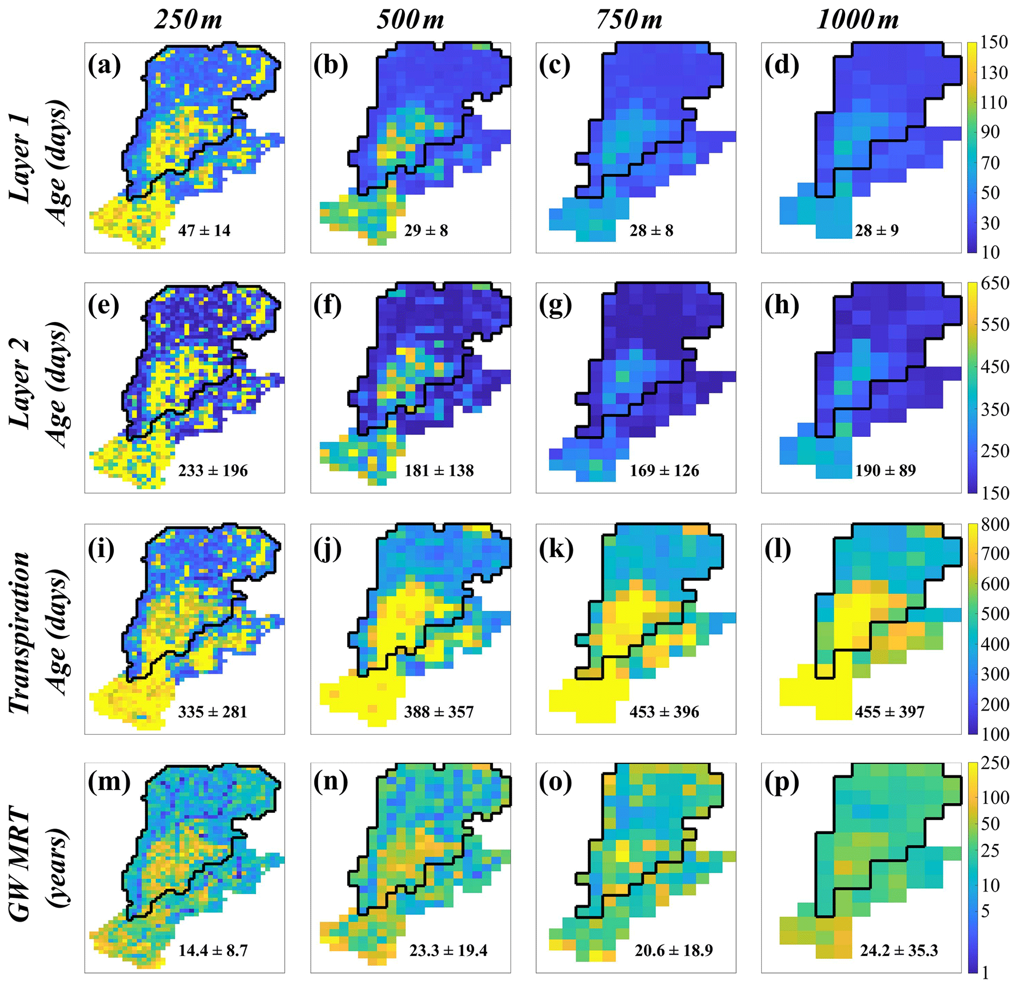
Figure 7 Estimated average water ages during the summer (June–August) in (a–d) soil layer 1 and (e–h) layer 2 and (i–l) transpiration and (m–p) long-term groundwater mean residence time (GW MRT) for model resolutions 250, 500, 750, and 1000 m, respectively. Note: groundwater residence times are in years. Black boundaries show the calibration extent of the Demnitz Mill subcatchment. Values shown are the catchment-wide, long-term (2009–2019) average values and average standard deviation (average of each pixel) within the Demnitz Mill subcatchment.

Unlike layers 1 and 2, the median and uncertainty of modelled transpiration and groundwater (GW) ages increased with model resolution (Fig. 7i–p). On average, transpiration water ages were slightly older than 1 year. GW ages were decadal at all resolutions, with an increase in GW age in the mid-reaches of the catchment. Spatial proximity of groundwater storages to streams was apparent at finer resolutions (Fig. 7m and n), with decreasing riparian GW ages in cells with streams. Transpiration water ages were much older with higher ET and much younger with higher recharge (Figs. 4 and 7). A similar strong increase in transpiration age was observed with proportions of conifers and peaty and podzolic soils and a strong decrease was observed with croplands and brown earth proportions (Fig. S5). Dependencies of GW ages on fluxes, storage, vegetation, and soils at all model resolutions were relatively limited. A consistent correlation of GW age was observed with recharge (strongly negative), the proportion of conifer forest (strongly positive), and gley soil (weakly negative).

Table 6 Estimated stream water ages (years) under high-flow anomaly (Q_a>1.0), normal flows ($-\mathrm{0.5}\le Q_{\mathrm{a}}\le \mathrm{1.0}$), and below-average-flow anomaly ($Q_{\mathrm{a}}\le -\mathrm{0.5}$) for Peat North, Peat South, Bruch Mill, and Demnitz Mill.

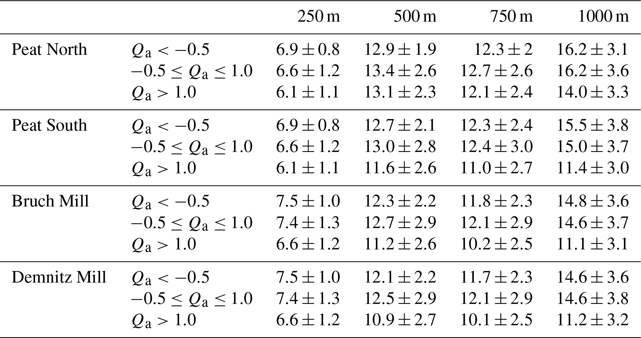
To characterise stream water ages during low-, medium-, and high-flow conditions, water ages were averaged for different flow conditions ($Q_{\mathrm{a}}=(Q-\stackrel{\mathrm{‾}}{Q})/\mathit{\sigma }$, where $\stackrel{\mathrm{‾}}{Q}$ is mean discharge, and σ is the standard deviation). High flow was defined as Q_a>1.0 and low flow as $Q_{\mathrm{a}}<-\mathrm{0.5}$. Similar to GW, modelled stream water ages and uncertainty increased with finer resolution (Table 6); however, stream water ages were notably younger than GW. At resolutions >250 m, stream water ages under all flow conditions moderately decreased from the headwaters (Peat North) to Demnitz Mill, whereas stream water ages increased downstream at the 250 m resolution. For all resolutions, high-flow conditions showed a notable decrease in stream water ages compared to the medium- and low-flow conditions (Table 6). During the largest events, stream water ages dropped most notably in the 750 and 1000 m resolutions (average stream water age of 0.5 years during peak events; Q_a≫1), reflecting extensive overland flow simulations (Table 6). Stream water ages for the finer grids also decreased during large events (average stream water age of 1.8 years during peak events, Q_a≫1); however, the change was not quite as large relative to the long-term average stream water age compared to coarse grids.

5 Discussion

5.1 Utility of tracer-aided ecohydrological models in constraining water storage–flux–age interactions at different spatial resolutions

This study demonstrated the effectiveness of a physically based, tracer-aided ecohydrological model in consistently simulating blue and green water fluxes and their relationships to vegetation, soil cover, and water storage in a 66 km² catchment across different spatial resolutions. The relatively minor variability in catchment-scale fluxes between model resolutions relative to model uncertainty is promising for the continued development of tracer-aided ecohydrological models for larger scales and spatial resolutions. This includes applications for a wide range of hydroclimatic conditions, including extreme droughts, where changes in blue and green flux partitioning can be marked (Prudhomme et al., 2014). Furthermore, the catchment-wide water balance and water loss, including leakance to the regional groundwater system, was consistent with simpler monthly water balance estimates for the catchment (Smith et al., 2020a). The larger areas of more homogenous land cover (e.g. croplands and conifer forests) consistently showed spatial patterns (Figs. 1 and 4) between model resolutions of lower ET and higher recharge in the croplands and a higher ET, a lower annual ratio of transpiration to ET (due to interception), and a lower recharge in the conifer forests. These catchment-scale results are consistent with findings of previous plot-scale studies in the region (Douinot et al., 2019; Smith et al., 2020b; Kleine et al., 2020). Interception evaporation is high in the conifer forests, likely due to the relatively consistent annual LAI in Scots pine plantations and the more frequent winter precipitation feeding interception storage. This is confirmed with higher transpiration to ET ratios during the summer months in the forests (Fig. S6). During the summer, greater interception capacity, lower evaporation resistance relative to transpiration, and drier soils than the croplands led to a more rapid turnover of interception storage, decreased available energy for transpiration within the canopy, and potentially more water-limited vegetation. Water limitation due to the sandy soils in the forested areas has been shown to suppress transpiration rates in the catchment (Smith et al., 2020b). While the transpiration to ET ratio is moderately low, it is within the range previously indicated by large-scale modelling (Sutanto et al., 2014). Similarly, parameterisations of the rooting zone were consistent across all resolutions for each vegetation type (Fig. S4), suggesting the calibration achieved an effective constraint for more consistent, larger-scale modelling of ecohydrological interactions. Model results for the wetlands in the mid-reaches of the catchment captured wet and saturated conditions across all resolutions, despite no direct soil moisture calibration in this area (Fig. 6). This suggests sufficient model skill in reproducing differences in moisture conditions where slight variations in topography cause marked ecohydrological contrasts.

One of the main advantages of tracer-aided models is capturing the distributions and dynamics of water storage involved in mixing processes that explain the damping and lagging of precipitation signals being transmitted through the system. At the catchment scale, all model resolutions reproduced a groundwater-dominated stream flow system that is driven by recharge in the headwaters. Thus, recharge is very sensitive to land cover and ecohydrological partitioning. As a result, the modelled catchment flow domain links relatively large, rapidly circulating and recharged sources of groundwater in the slightly steeper headwaters under crops to shallower stores of older groundwater under forests that receive much lower recharge (Figs. 6 and 7). Near-surface water storage is greatest in the wetland areas where younger water can contribute to streamflow as localised overland flow in wet periods; however, this was only reproduced at the two finer model resolutions. Thus, while the dynamics and totals of blue and green fluxes and water storage–flux–age interactions of dominant vegetation and soils (e.g. croplands and brown earth and conifers and podzols) were relatively consistent between model resolutions (Fig. 4), there were differences in localised hydrologically important vegetation–soils grids at different grid scales. This probably reflects calibration not capturing subtle, but important, differences in the representations of modelled flow paths at coarser resolutions (Blöschl and Sivapalan, 1995; Harvey, 2000; Vereecken et al., 2007). For example, limited variability in stream isotopes, older groundwater, and stream water ages observed at model resolutions greater than 500 m are consistent with a loss of smaller-scale process representation (Figs. 3 and 7).

These latter differences in process representation likely reflect interactions in the deeper soils, and between groundwater and the stream network, as water storage and ages at all resolutions in layers 1 and 2, as well as soil evaporation ages, were consistent with those estimated in other, similar catchments (e.g. Douinot et al., 2019) and plot-scale modelling in the DMC (Smith et al., 2020b).

Modelled groundwater ages at finer resolutions (250 and 500 m) were more consistent with local groundwater tritium age dating and, similarly, showed a decrease in groundwater age in closer proximity to stream channels (Massmann et al., 2009). In contrast, coarser resolutions produced older, more spatially uniform water ages. Finer model resolutions additionally showed spatial patterns of groundwater inflows to streams (not shown) in locations that were consistent with the historical distribution of wetlands and ponded areas prior to drainage (Gelbrecht et al., 2005). This suggests a dissociation of some important hydrological processes in riparian areas at coarser scales, including localised overland flow in wetlands which contributes to runoff peaks in winter and associated isotope variations (e.g. Grabs et al., 2012). This probably contributed to the loss of tracer dynamics as aggregation more coarsely represents storage–flux–age interaction due to averaging of spatial heterogeneity of vegetation and soil and subsurface properties (Ershadi et al., 2013; Yang et al., 2001).

5.2 How do coarser model resolutions affect uncertainty and model parameter sensitivity?

Changes in parameter sensitivity and posterior parameter ranges with model resolution provide key information on internal process representation that can help reduce the degrees of freedom and increase model robustness (Blöschl and Sivapalan, 1995). The broadly consistent ranking of sensitive parameters for each resolution (Fig. 2) suggests that the model parameters performed similarly across different grid scales, albeit with slightly less sensitivity for individual parameters at coarser resolutions. Discharge showed the most notable decrease in sensitivity across resolutions, driven by the scaling of Manning's n (Fig. S3). The sensitivity of Manning's n across resolutions is nonlinear, accounting for changes in numerical wave routing (Courant criteria), channel length, roughness, and shape in larger resolutions (similar to Bhaskar et al., 2015). In soils (soil moisture), deviations in parameter sensitivity and uncertainty across resolutions are likely due to the aggregation of topographic features (e.g. slope) which can change the details of groundwater movement and distribution of saturation areas surrounding the stream (e.g. Yang et al., 2001). Vegetation properties generally control the sensitivity of the energy balance (particularly LE), which is unsurprising given the dependence of remote sensing LE estimations on vegetation coverage (e.g. Mu et al., 2011). The low sensitivity of energy balance components to soils is likely due to low soil evaporation (soil latent heat) and outgoing shortwave (low albedo) contributions.

Evaluation of catchment flux–storage–age representations with finer resolutions resulted in significantly better model efficiencies (average 20 % improvement with the 250 m resolution compared to all others), with an apparent threshold between 250 and 500 m (Fig. S2). The better model efficiency at finer resolutions may be due to either a spatial threshold of calibration data (e.g. measured soil moisture) for coarse resolutions (limiting efficiency) or a loss of dynamics in larger grids due to the aggregation of fine-scale landscape characteristics (Samaniego et al., 2017). Additionally, the lower efficiency at coarser scales (e.g. stream isotopes) may be due to trade-offs between optimising outputs that fit poorly (especially stream isotopes) and outputs that fit well in multicriteria calibration (Efstratiadis and Koutsoyiannis, 2010). However, it should be noted that even simulations of general isotope values in streamflow, despite the loss of short-term dynamics, are still likely much more indicative of reasonable catchment-scale storage–flux estimates than a model not using tracers (Birkel et al., 2011; Holmes et al., 2020).

As with efficiency, uncertainty, in terms of the range of upper and lower simulation bounds, improved (decreased) with finer resolutions. In addition to wider simulation bounds at calibrated sites, coarser scales revealed larger variability, particularly in stream isotope and water age simulations. The large variability suggests, consistent with the comments in Sect. 5.1, that key processes (i.e. local overland flow and groundwater fluxes) and isotopic mixing (wetland isotopic mixing) are not well constrained (Tetzlaff et al., 2017; Kuppel et al., 2018). The increased uncertainty and variability is particularly notable in the groundwater age for coarse resolutions, which is more than 4 times larger than finer resolutions (Fig. 7). The high uncertainty at coarser scales complicates the evaluation of the storage to buffer climatic change (Kløve et al., 2014) or water quality impacts (Hill, 2019). However, the primary differences in uncertainty between model resolutions appeared to be mainly restricted to isotope and water age estimations, as catchment average variability were similar across resolutions for ecohydrological fluxes (e.g. Figs. 4 and 6).

5.3 Implications of field data, remote sensing data, and data fusion data sets for limitations on large-scale modelling

Evaluation of how ecohydrological fluxes, storages, and water ages and their uncertainties upscale from smaller, nested field sites to larger scales is useful for coupling with regional climate models and is essential for science to inform management, as policy focuses on larger scales with broader implications on societal water demands and usage (Asbjornsen et al., 2011). To better understand how well feedback mechanisms between soil, vegetation, and the atmosphere are captured in modelling at various scales, long-term and multiscale data collection is required, particularly for soil moisture, due to the strong influence of vegetation on soil moisture dynamics (Asbjornsen et al., 2011; Vereecken et al., 2019). Here, multiple soil moisture measurements in various soil–vegetation systems were useful in constraining model calibration, with a stronger influence at finer scales (Table 4). In addition, other high-resolution data (e.g. spatial resolution for isotopes and temporal resolution for sap flow) proved beneficial for calibration at the catchment scale, highlighting the value of long-term data collection in experimental catchments (Tetzlaff et al., 2017). Stream isotopes were of primary importance in revealing differences in model process fidelity and reducing the uncertainty of flow path representation. In particular, processes in key hydrologic “hot spots” (e.g. 2.8 km² wetland between Peat North and Peat South) were constrained solely by stream and groundwater isotope field data. Isotopic data likely helped to constrain the calibration, especially regarding the evaporative enrichment and mixing in the wetland (Sprenger et al., 2017). However, there was an apparent scale limit to the value of isotope field data in capturing more localised processes with coarser scales too large to adequately capture important wetland processes. This example suggests an “upscaling process limit” for isotopic impacts and a representative elementary area between 500 and 750 m for the DMC (Wood et al., 1988; Blöschl and Sivapalan, 1995), with a maximum representative grid resolution of 500 m for the grid sizes tested in this study. For all resolutions, the shorter time series for water stable isotopes resulted in gaps in key calibration periods and larger uncertainty when data were not available (Fig. 5e–h). Additionally, the model was able to adequately reproduce stream isotopes at a single location (Table S1); however, processes were only fully constrained with the multicriteria calibration of all stream isotope locations. These data limitations highlight the value of spatially distributed long-term data to drive model improvements (Soulsby et al., 2015).

These inevitable limitations in the availability of long-term data emphasise the inherent advantages of remotely sensed data. While the remote sensing data were essential for constraining the catchment-wide ET and LE (8 d and annual amounts), the limited heterogeneity in the coarser-scale remote sensing products (Table 1) resulted in a poorer fit at finer resolutions, which had more spatial heterogeneity at key field-scale measurement sites. The lower calibration efficiency criteria of finer resolutions to remotely sensing ET and LE estimations is likely due to scaling in the latter. The relatively coarse grid resolution of the MODIS ET and LE data aggregates multiple land cover types into each grid, which is known to result in large uncertainties in daily and monthly ET estimates (Gowda et al., 2007; Velpuri et al., 2013). Additionally, at finer resolutions, the lower modelled soil wetness relative to coarser resolutions restricted ET and LE, relative to MODIS estimations (i.e. lower annual ET and model ET efficiency), which estimates ET and LE from vegetation coverage (Mu et al., 2011). Lower ET and LE have also been seen at the plot-scale during dry years (Smith et al., 2020b). Of the calibrated vegetation ET, the conifer forests were the most different from MODIS data (Table 4) for various reasons. The dependence of MODIS ET on vegetation coverage may be influenced by underlying errors in overestimating LAI variability in conifer and broadleaf forests due to uncertainties in atmospheric correction (Heiskanen et al., 2012), leaf optical characteristics during leaf out and senescence (Wang et al., 2005), and over-compensation of understory canopy development (Jensen et al., 2011). However, these underlying errors and limited dependencies on soil wetness are likely minimised on an annual basis and under average precipitation (e.g. similar catchment-wide ET between model resolutions; Fig. 4). The fusion of additional products (e.g. Landsat and Sentinel-2) may further alleviate some interannual uncertainties of remote sense data sets; however, extreme conditions still require ground truthing, underlining the need for data-rich experimental catchments.

6 Conclusions

Long-term water security is dependent on quantitative knowledge of regional water storages and fluxes and how these are anticipated to change under the anticipated increased frequency of extreme events, such as droughts (Falkenmark and Rockström, 2006). However, how the vegetation–soil–atmosphere interactions regulating ecohydrologic fluxes that are additionally expected to change is not well known. This is particularly the case at larger scales, resulting in an uncertain evidence base for land use decision-making in regions where water resources are under stress (e.g. agricultural areas; Falkenmark and Rockström, 2010). The significant challenges at larger scales are tied to the limitations of appropriately upscaling the controlling of vegetation–soil interactions in models between spatial scales.

The physically based tracer-aided ecohydrologic model EcH₂O-iso allowed us to assess the effects of spatial interactions across model scales, using four resolutions of the same 66 km² catchment in northeastern Germany. This used multicriteria calibration of field data (discharge, soil moisture, stream, and soil isotopes) and remotely sensed data in a data fusion approach. Fluxes and water storages were reproduced similarly across all model resolutions, with the dominant soil and vegetation covers largely explaining the spatial distributions. Identification of sensitive parameters was similar across scales; however, a notable decrease in the degree of sensitivity, coupled with an increase in all model output uncertainty, occurred with coarser model resolutions. Isotopic and water age simulations revealed limitations at larger spatial resolutions for internal mixing mechanisms, most notably surface runoff, wetland evaporation, and deeper groundwater mixing. Despite this, for all model scales, spatially distributed data sets of both remote sensing products and more local field data (particularly isotopes) were useful calibration constraints in modelling ecohydrological fluxes, while also giving a plausible representation of water storage and age interactions at the catchment scale. The effectiveness of the model for simultaneously capturing ecohydrologic fluxes, storages, and age interactions for each resolution provides a promising basis for further testing of upscaling spatio-temporal influences of soil–vegetation–atmospheric interactions in larger catchments.