the Creative Commons Attribution 4.0 License.
the Creative Commons Attribution 4.0 License.
 | 22 Apr 2021
Technical note: Diagnostic efficiency – specific evaluation of model performance
Robin Schwemmle
Dominic Demand
Markus Weiler
A better understanding of the reasons why hydrological model performance is unsatisfying represents a crucial part of meaningful model evaluation. However, current evaluation efforts are mostly based on aggregated efficiency measures such as Kling–Gupta efficiency (KGE) or Nash–Sutcliffe efficiency (NSE). These aggregated measures provide a relative gradation of model performance. Especially in the case of a weak model performance it is important to identify the different errors which may have caused such unsatisfactory predictions. These errors may originate from the model parameters, the model structure, and/or the input data. In order to provide more insight, we define three types of errors which may be related to their source: constant error (e.g. caused by consistent input data error such as precipitation), dynamic error (e.g. structural model errors such as a deficient storage routine) and timing error (e.g. caused by input data errors or deficient model routines/parameters). Based on these types of errors, we propose the novel diagnostic efficiency (DE) measure, which accounts for these three error types. The disaggregation of DE into its three metric terms can be visualized in a plain radial space using diagnostic polar plots. A major advantage of this visualization technique is that error contributions can be clearly differentiated. In order to provide a proof of concept, we first generated time series artificially with the three different error types (i.e. simulations are surrogated by manipulating observations). By computing DE and the related diagnostic polar plots for the reproduced errors, we could then supply evidence for the concept. Finally, we tested the applicability of our approach for a modelling example. For a particular catchment, we compared streamflow simulations realized with different parameter sets to the observed streamflow. For this modelling example, the diagnostic polar plot suggests that dynamic errors explain the overall error to a large extent. The proposed evaluation approach provides a diagnostic tool for model developers and model users and the diagnostic polar plot facilitates interpretation of the proposed performance measure as well as a relative gradation of model performance similar to the well-established efficiency measures in hydrology.
- Article
(2103 KB) - Full-text XML
-
Supplement
(583 KB) - BibTeX
- EndNote


Performance metrics quantify hydrological model performance. They are employed for calibration and evaluation purposes. For these purposes, the Nash–Sutcliffe efficiency (NSE; Nash and Sutcliffe, 1970) and the Kling–Gupta efficiency (KGE; Gupta et al., 2009) are two commonly used performance metrics in hydrology (e.g. Newman et al., 2017; Towner et al., 2019). NSE and KGE measure the overall model performance with only a single numerical value within the range of minus infinity and one. A value close to one indicates a better model accuracy, whereas with increasing distance to one the model accuracy deteriorates. From this point of view, the model performance can only be assessed in terms of a relative gradation. However, cases of a weaker model performance immediately lead to the following questions: why is my model performance not satisfactory? What could improve the model performance?
In order to answer such questions, Gupta et al. (2008) proposed an evaluation approach that includes diagnostic information. Such a diagnostic approach requires appropriate information. Considering only the overall metric values of NSE and KGE may not provide any further insights. Additionally, an in-depth analysis of KGE metric terms may provide more information on the causes of the model error (e.g. Towner et al., 2019). Although including the KGE metric terms may enrich model evaluation, due to their statistical nature the link to the hydrological process is less clear. Current diagnostic approaches are either based on entropy-based measures (Pechlivanidis et al., 2010) or on process-based signatures (Yilmaz et al., 2008; Shafii et al., 2017). The latter one improves measurement of the realism of hydrological processes by capturing them in hydrological signatures. These signatures represent a main element of a powerful diagnostic approach (Gupta et al., 2008).
Although the numerical value of the overall model performance is diagnostically not meaningful, the overall model performance determines whether diagnostic information will be valuable to the modeller or not. Diagnostic information may only be useful if the overall model performance does not fulfil the modeller's requirements. It will then be cumbersome to select the appropriate signatures or measures which may answer the modeller's questions about the causes. Visualizing evaluation results in a comprehensive way poses another challenge for diagnostically meaningful interpretation. Therefore, we see a high potential in compressing the complex error terms into one diagram simplifying the interpretation and the comparison of multiple simulations. In this study, we propose a specific model evaluation approach with a strong focus on the error identification which contributes to existing diagnostic evaluation approaches and builds on existing approaches.
2.1 Diagnostic efficiency
In general, the quality of evaluation data (e.g. streamflow observations) should be verified before simulations and observations are compared against each other. Model evaluation data with insufficient accuracy should not be considered for model evaluation (e.g. Coxon et al., 2015). Likewise, accuracy of initial and boundary conditions should be inspected beforehand (e.g. Staudinger et al., 2019). Remaining errors in hydrological simulations may then be caused by the following sources:
-
model parameters (e.g. Wagener and Gupta, 2005);
-
model structure (e.g. Clark et al., 2008, 2011);
-
uncertainties in input data (e.g. Yatheendradas et al., 2008).
Thus, within our approach we focus on errors caused by model parameters, model structure, and input data. In order to diagnose the source of the errors, we define three error types which might be linked to potential error sources (e.g. model parameters, model structure, and input data): (i) constant error describes the average deviation between simulations and observations; (ii) dynamic error defines the deviation at different simulated and observed magnitudes; and (iii) timing error comprises the temporal agreement between simulations and observations. Model errors may have different sources. Assigning the error type to its source requires expert knowledge (e.g. shortcomings of the input data) or statistical analysis (e.g. linking the error types with the model parameters). We provide here some examples of how expert knowledge might be used to link the input data with the error type. A constant error might be linked to the precipitation input; for example, Beck et al. (2017) found negative constant errors in snow-dominated catchments. In case the precipitation input error varies between rainfall events, the input data might be the source of dynamic errors (e.g. Yatheendradas et al., 2008). On the other hand, errors in the spatio-temporal rainfall pattern might be the source of timing errors (e.g. Grundmann et al., 2019).
In order to quantify the overall error, we introduce the diagnostic efficiency (DE; Eq. 1):
where is a measure for the constant error, for the dynamic error, and r for the timing error. DE ranges from 0 to ∞ and DE=0 indicates that there are no errors (i.e. perfect agreement between simulations and observations). In contrast to KGE and NSE, DE represents an error score. This means that model performance is decreasing for increasing values of DE.
First, we introduce the three terms which define the DE. The first two terms and are based on the flow duration curve (FDC). Since FDC-based signatures do not include information on temporal performance, we have added correlation (r) between the simulated time series and the observed time series as a third term. reflects the constant error and is represented by the arithmetic mean of the relative bias (Eq. 2):
i represents the exceedance probability, N the total number of data points, and Brel the relative bias of the simulated and observed flow duration curve; indicates no constant error; indicates a negative bias; indicates a positive bias. The relative bias between the simulated and observed flow duration curve (Brel) is calculated as follows (Eq. 3):
Qsim is the simulated streamflow at exceedance probability i and Qobs the observed streamflow at exceedance probability i. Due to Eq. (3) the presented approach is only applicable to regions with perennial streamflow.
The dynamic error is described by the absolute area of the residual bias (; Eq. 4):
where the residual bias Bres is integrated over the entire domain of the flow duration curve. Combining Eqs. (2) and (3) results in
By subtracting , we remove the constant error, and the dynamic error remains. indicates no dynamic error; indicates a dynamic error.
To consider timing errors, Pearson's correlation coefficient (r) is calculated (Eq. 6):
where Qsim is the simulated streamflow at time t, Qobs the observed streamflow at time t, μobs the simulated mean streamflow, and μobs the observed mean streamflow. Other non-parametric correlation measures could be used as well.
2.2 Diagnostic polar plot
DE can be used as another aggregated efficiency by simply calculating the overall error. However, the aggregated value only allows for a limited diagnosis since information of the metric terms is not interpreted. Thus, we project DE and its metric terms in a radial plane to construct a diagnostic polar plot. An annotated version for a diagnostic polar plot is given in Fig. 3. For the diagnostic polar plot, we calculate the direction of the dynamic error (Bdir; Eqs. 7–9):
where Bhf is the integral of Brel including values from 0th percentile to 50th percentile and Blf is the integral of Brel including values from 50th percentile to 100th percentile. Since we removed the constant error (see Eq. 5), the integrals can be positive, negative, or zero.
In order to differentiate the dynamic error type, we computed the slope of the residual bias (Bslope; Eq. 10):
Bslope=0 expresses no dynamic error; Bslope<0 indicates that there is a tendency of simulations to overestimate high flows and/or underestimate low flows, while Bslope>0 indicates a tendency of simulations to underestimate high flows and/or overestimate low flows.
To distinguish whether the constant error and the dynamic error are more related to high flows (i.e. 0th percentile to 50th percentile) or to low flows (i.e. 50th percentile to 100th percentile), we quantify their contribution. For this we calculate the error contribution of high flows (εhf; Eq. 11) and low flows (εlf; Eq. 12):
where Bhf is the area of the relative bias for high flows, Blf is the area of the relative bias for low flows, and Btot is the absolute area of the relative bias.
We used the inverse tangent to derive the ratio between constant error and dynamic error in radians (ϕ; Eq. 16):
Instead of using a benchmark to decide whether model diagnostics is valuable or not, we introduce a certain threshold for deviation from perfect. We set a threshold value (l) for which metric terms deviate from perfect and insert it into Eq. (1):
For this study l is set by default to 0.05. Here, we assume that for a deficient simulation each metric term deviates at least 5% from its best value; l can be either relaxed or expanded depending on the requirements of model accuracy. Correspondingly, DEl represents a threshold to discern whether an error diagnosis (DE > DEl) is valuable.
Finally, the following conditions describe whether a diagnosis can be drawn (Eq. 18):
There exists a special case for which timing error only can be diagnosed (Eq. 19):
If DE and its metric terms are within the boundaries of acceptance, no diagnosis is required, which is expressed by the following conditions (Eq. 20):
In this case, the model performance is sufficiently accurate, and errors are too small.
2.3 Comparison to KGE and NSE
In order to allow a comparison to commonly used KGE and NSE, we calculated the overall metric values and, for KGE, its three individual metric terms. We used the original KGE proposed by Gupta et al. (2009):
where β is the bias error, α represents the flow variability error, and r shows the linear correlation between simulations and observations (Eq. 22):
where σobs is the standard deviation in observations and σsim the standard deviation in simulations. Moreover, we applied the polar plot concept (see Sect. 2.2) to KGE and the accompanying three metric terms. In contrast to DE (see Sect. 2.1), KGE ranges from 1 to −∞ and the metric formulation of KGE is entirely based on statistical signatures. By replacing the first two terms of KGE with FDC-based signatures, we aim to improve the hydrological focus and provide a stronger link to hydrological processes (e.g. Ghotbi et al., 2020).
NSE (Nash and Sutcliffe, 1970) is calculated as follows (Eq. 23):
where T is the total number of time steps, Qsim the simulated streamflow at time t, and Qobs the observed streamflow at time t and μobs. NSE=1 displays perfect fit between simulations and observations; NSE=0 indicates that simulations perform equally well as the mean of the observations; NSE<0 indicates that simulations perform worse than the mean of the observations.
To provide a proof of concept, any perennial streamflow time series coming from a near-natural catchment and having a sufficiently long temporal record (i.e. >30 years) may be used. We selected an observed streamflow time series from the CAMELS dataset (Fig. 1; Addor et al., 2017). In order to generate specific model errors, we systematically manipulated the observed time series. Thus, we produced different time series which serve as a surrogate for simulated time series with a certain error type which we call manipulated time series. These manipulated time series are characterized by a single error type or multiple error types, respectively. We calculated DE for each manipulated time series and visualized the results in a diagnostic polar plot.
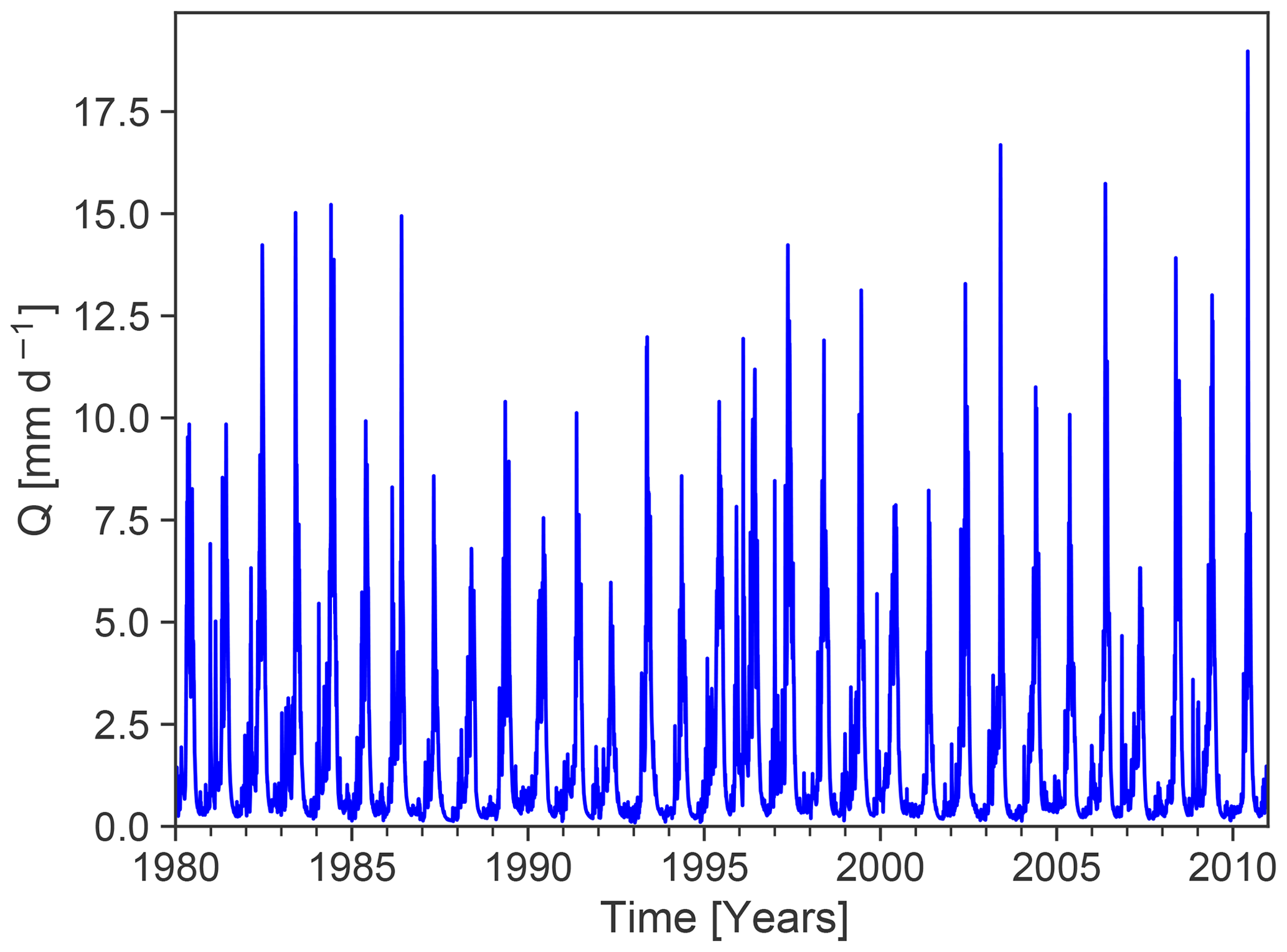
Figure 1Observed streamflow time series from the CAMELS dataset (Addor et al., 2017; gauge id: 13331500; gauge name: Minam River near Minam, OR, US).
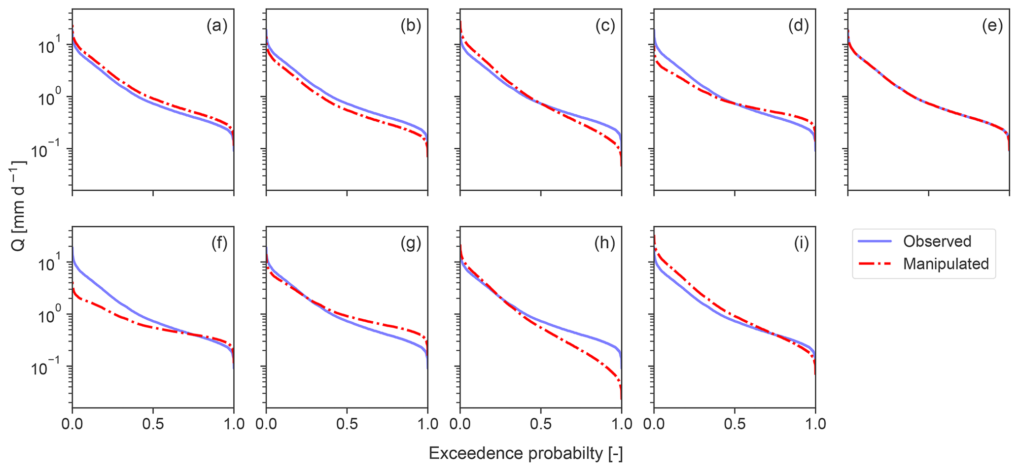
Figure 2Flow duration curves (FDCs) of observed (blue) and manipulated (dashed red) streamflow time series. Manipulated FDCs are depicted for (a, b) constant errors only, (c, d) dynamic errors only, (e) timing error only, and (f–i) combination of dynamic and constant errors. The combination of constant errors, dynamic errors, and timing error is not shown, since their FDCs are identical to (f)–(i). Y axis is shown in log space.
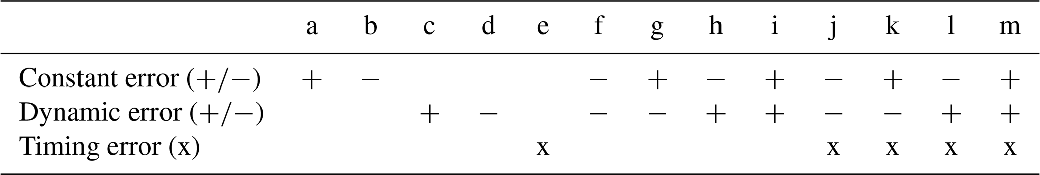
Table 1Summary of error types and their combinations as described in Sect. 3.1 (a–m). + (−) reflects a positive (negative) error type. For timing error, only one error type exists (x).
3.1 Generation of artificial errors
In the following section, we portray how we manipulated observed time series to generate artificial modelling errors. Table 1 provides a brief summary of the error types and how we combined them. The resultant FDCs are illustrated in Fig. 2. For the corresponding time series, we refer to the Supplement (Fig. S1). We first describe the genesis of the time series for individual errors.
- a.
Positive constant error: we generated a positive offset by multiplying the observed time series by a constant 1.25 (see Figs. 2a and S1a). Constant required to be >1.
- b.
Negative constant error: we generated a negative offset by multiplying the observed time series by a constant 0.75 (see Figs. 2b and S1b). Constant required to be <1.
- c.
Positive dynamic error: we built a linearly interpolated vector (1+p, …, 1, …, p) with p set to 0.5. We then generated the error by multiplying the observed FDC by the linearly interpolated vector. With that we increased high flows and decreased low flows. As a consequence, hydrological extremes are amplified (see Figs. 2c and S1c). Note that the original temporal order of the time series is maintained.
- d.
Negative dynamic error: we built a linearly interpolated vector (p, …, 1, …, 1+p) with p set to 0.5. We then generated the error by multiplying the observed FDC by the linearly interpolated vector. With that we decreased high flows and increased low flows. As a consequence, hydrological extremes are moderated (see Figs. 2d and S1d). Note that the original temporal order of the time series is maintained.
- e.
We reproduced a timing error by randomizing the order of the observed time series (see Figs. 2e and S1e).
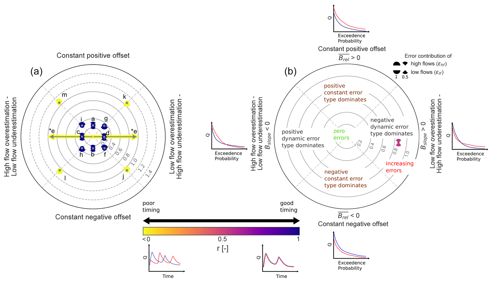
Figure 3(a) Diagnostic polar plot for manipulated time series generated characterized by constant errors, dynamic errors, and timing errors (a–m) visualizing the overall model performance (DE; contour lines) and contribution of constant error, dynamic error, and timing error – purple (yellow) indicates temporal match (mismatch). The error contribution of high flows and low flows is displayed by pies. (e*) Timing error only: type of dynamic error cannot be distinguished. (b) Annotated diagnostic polar plot illustrating the interpretation (similar to Zipper et al., 2018). Hypothetic FDC plots and hydrograph plots give examples of the error types.
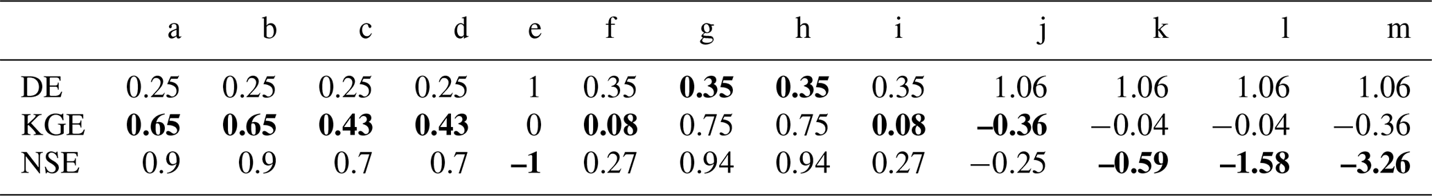
Table 2Comparison of DE, KGE and NSE calculated for manipulated time series characterized by constant errors, dynamic errors and timing errors (a–m). Lowest model performance for each error case is in bold.
We then assembled the individual techniques (a–d) for the genesis of time series which are characterized by a combination of constant error and dynamic error. The two errors contribute with an equal share,
- f.
negative constant error and negative dynamic error (see Figs. 2f and S1f),
- g.
positive constant error and negative dynamic error (see Figs. 2g and S1g),
- h.
negative constant error and positive dynamic error (see Figs. 2h and S1h),
- i.
positive constant error and positive dynamic error (see Figs. 2i and S1i),
and time series which contain constant error, dynamic error (again both errors are contributing with an equal share), and timing error (a–e):
- j.
negative constant error, negative dynamic error and timing error (see Fig. S1j);
- k.
positive constant error, negative dynamic error and timing error (see Fig. S1k);
- l.
negative constant error, positive dynamic error and timing error (see Fig. S1l);
- m.
positive constant error, positive dynamic error and timing error (see Fig. S1m).
Note that for j–m FDCs are identical to f–i and are therefore not shown in Fig. 2.
The diagnostic polar plot for synthetic error cases is shown in Fig. 3. Since each synthetic error case is different, related points are located in different error regions. For individual errors (a–d), related points are placed in the four cardinal directions of each region (Fig. 3). Within these regions the dominant error type can be easily identified. The more central the direction of the point, the more dominant the error type. In case there is only a timing error present (e), an arrow with two ends instead of a point is used (Fig. 3). This is because the dynamic error source becomes arbitrary (i.e. high flows and low flows are being both underestimated and overestimated; see Fig. S1e). For combinations of constant and dynamic errors (f–i), related points are located on boundaries of constant error and dynamic error, meaning that both errors are equally dominant (Fig. 3). The same applies for combinations of constant error, dynamic error, and timing error except that points shifted towards the outer scope of the plot due to added timing error. Numeric values of DE are listed in Table 2. DE values are lower for individual errors (except for the timing error) than for combined errors. Increasing the number of errors added to a time series leads to greater DE values. For the numeric values of the individual metric terms, we refer to Table S1 in the Supplement.
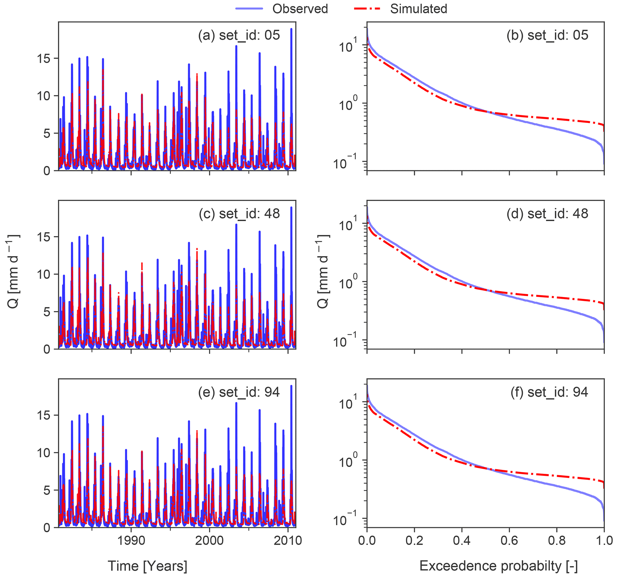
Figure 4Simulated and observed streamflow time series of modelling examples for the year 2000 (a, c, e) and the related flow duration curves for the entire time series (b, d, f). Time series are derived from the CAMELS dataset (Addor et al., 2017). Observations and simulations belong to the same catchment as in Fig. 1. Simulations were produced by model runs with different parameter sets (set_id) but same input data (see Newman et al., 2015).
A comparison of DE, KGE, and NSE calculated for the manipulated time series is shown in Table 2. Moreover, values for DE exhibit a regular pattern (i.e. generating single error types or multiple error types, respectively, leads to an equidistant decrease in performance). By contrast, values for KGE and NSE are characterized by an irregular pattern (i.e. generating single error types or multiple error types, respectively, leads to a non-equidistant decrease in performance). This non-equidistant decrease in KGE and NSE scores suggests that KGE and NSE are differently sensitive to the generated errors. KGE is more sensitive to constant errors and dynamic errors (Table 2, a–d), whereas NSE is more sensitive to timing errors (Table 2, e). Particularly, the spurious timing of the peak flows leads to an strong decrease in NSE (Table 2, m). When combining positive constant error and negative dynamic error, and vice versa (see Table 1, g and h), KGE and NSE display better performance (Table 2, g and h) than for single constant and dynamic error types (Table 2, a–d).
3.2 Modelling example
In order to demonstrate the applicability, we also use simulated streamflow time series which have been derived from Addor et al. (2017). Streamflow time series have been simulated by the coupled Snow-17 and SAC-SMA system for the same catchment as in Fig. 1. We briefly summarize here their modelling approach consisting of Snow-17, which “is a conceptual air-temperature-index snow accumulation and ablation model” (Newman et al., 2015), and the SAC-SMA model, which is “a conceptual hydrologic model that includes representation of physical processes such as evapotranspiration, percolation, surface flow, and subsurface lateral flow” (Newman et al., 2015). Snow-17 runs first to partition precipitation into rain and snow and delivers the input for the SAC-SMA model. For further details about the modelling procedure, we refer to Sect. 3.1 in Newman et al. (2015). In particular, we evaluated three model runs with different parameter sets but the same input data. Simulated time series and simulated FDCs are shown in Fig. 4. The diagnostic polar plot for the three simulated time series is provided in Fig. 5. Simulations realized by a parameter set with set_id 94 outperform the other two parameter sets. All simulations have in common that positive dynamic error type (i.e. high flows are underestimated and low flows are overestimated) dominates, accompanied by a slight positive constant error. In particular, low flows have a greater share of the dynamic error and constant error than high flows. Timing contributes least to the overall error. The modelling example highlights one advantage of the proposed evaluation approach that multiple simulations can be easily compared to each other. For the case of the modelling example, model performance of slightly different parameter sets can be clearly distinguished, although the parameter sets are characterized by a similar error type. After identifying the error type and its contributions, these results can be used in combination with expert knowledge (e.g. model developer) or statistical analysis to infer hints on improving the simulations.
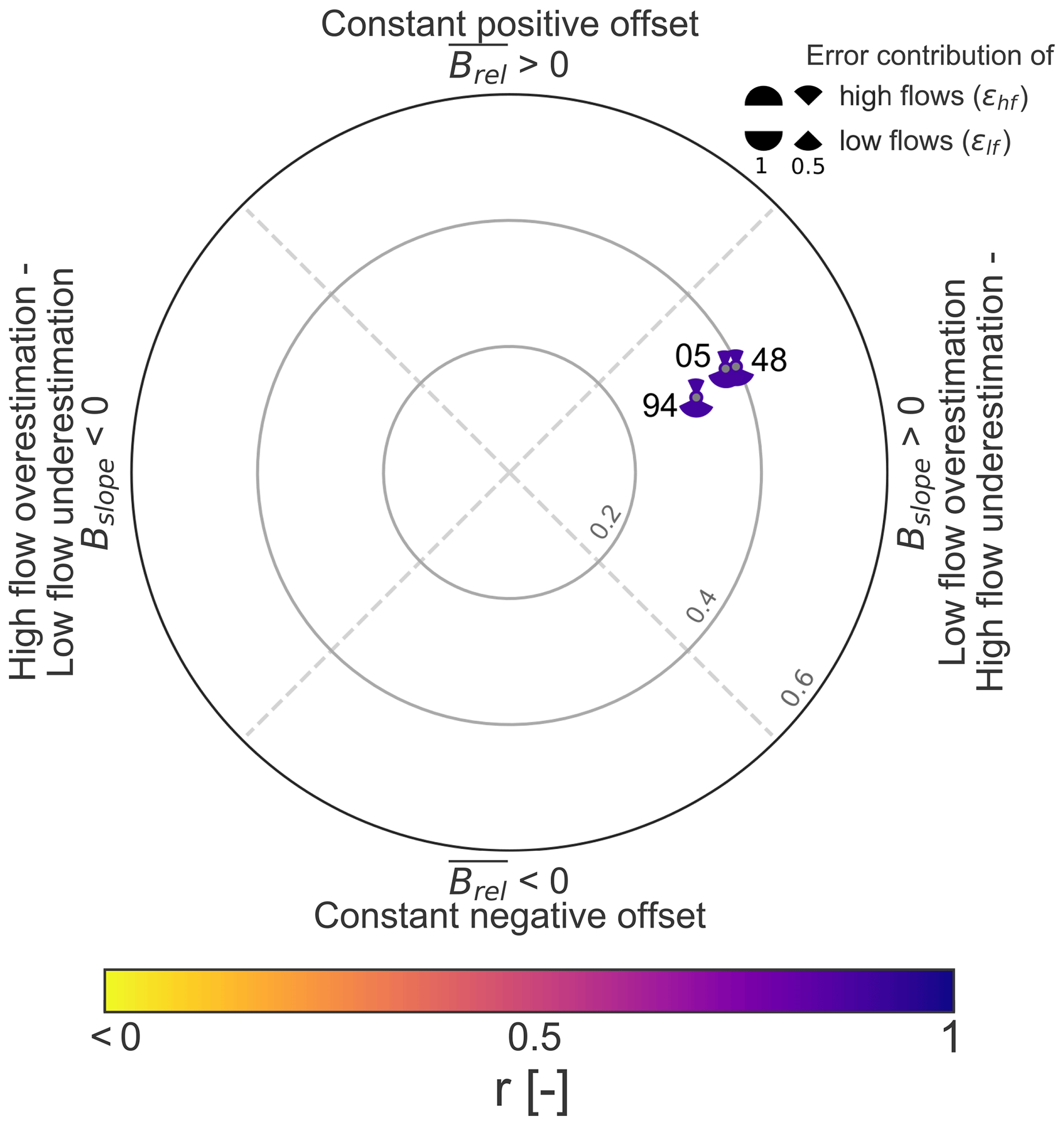
Figure 5Diagnostic polar plot for the modelling example. Simulations were realized with three different parameter sets (05, 48, 94; see Fig. 4). All simulations perform well. However, the remaining error is dominated by a negative dynamic error type, while timing is excellent.
Aggregated performance metrics (e.g. KGE and NSE) are being criticized for not being hydrologically informative (Gupta et al., 2008). Although we systematically generated errors, we found a disjointed pattern for KGE and NSE (Table 2) which makes the interpretation of KGE and NSE more difficult. Particularly, in-depth analysis of the KGE metric terms revealed that the β term and α term are not orthogonal to each other (see Figs. S2 and S3c). We also lump model performance into a single value, but DE has the following advantages: (i) metric formulation is based rather on a hydrological understanding than a purely statistical understanding; (ii) the combined visualization of the efficiency metric and the different metric terms enables the identification of the dominant error type; (iii) diagnostic polar plots facilitate comparison of multiple simulations. Using DE as an error score improves the interpretation of the numerical value. DE equals zero can be cleanly interpreted as zero errors. Additionally, numerical values of the first and second metric terms of DE equal to zero can also be interpreted as zero errors. Compared to KGE, the included FDC-based measures may be more easily linked to different hydrologic processes than purely statistical measures. For example, slow-flow processes (e.g. baseflow) control the low-flow segment of the FDC, while fast-flow processes (e.g. surface runoff) control the high-flow segment of the FDC (Ghotbi et al., 2020). When using KGE and NSE for evaluation purposes, we recommend a comparison to hydrologically meaningful benchmarks which may add diagnostic value to KGE (e.g. Knoben et al., 2019) and NSE (e.g. Schaefli and Gupta, 2007). Based on such a benchmark, skill scores have been recently proposed to evaluate simulations (Knoben et al., 2019; Towner et al., 2019; Hirpa et al., 2018) to communicate model performance and to improve hydrologic interpretation. So far a way to define hydrologically meaningful benchmarks has not been extensively addressed by the hydrologic modelling community (Knoben et al., 2019).
Our approach focuses on model errors. Since the DE can be interpreted as an error score, we do not propose a skill score measure for DE. Skill scores are known to introduce a scaling issue on communicating model errors (Knoben et al., 2019). DE does not rely on any benchmark to decide whether model diagnostics are required or not. Without considering any benchmark, DE may be interpreted as a deviation from perfect, measured by its constant error, dynamic, and temporal error terms. In Sect. 2.2 (see Eq. 17) we introduced a certain threshold for deviation from perfect (e.g. DE=0.09) if all error terms deviate by a certain degree (e.g. 5 %; , , r=0.95). Only for simulations in which deviation from perfect is sufficiently large will model diagnostics be valuable.
By including FDC-based information in DE, we aimed for capturing rainfall-runoff response behaviour (Vogel and Fennessey, 1994) where different aspects of the FDC are inherently related to different processes (Ghotbi et al., 2020). However, the way the dynamic error term is calculated (see Eqs. 4, 5, and 7) limits the applicability to catchments with perennial streamflow. Moreover, the second metric term of DE (see Eq. 1) is limited to measuring only the overall dynamic error. The question whether high-flow errors or low-flow errors are more prominent cannot be answered. Measuring the timing error by linear correlation may also have limitations. Linear correlation can be criticized for neglecting specific hydrological behaviour (Knoben et al., 2019), for example, flow recession or peak flow timing. However, DE could also be calculated for different time periods, and hence specific periods (e.g. wet periods versus dry periods) could be diagnosed separately.
Combining DE and diagnostic polar plots is, however, limited to three metric terms, because higher-dimensional information cannot be effectively visualized by polar plots. We emphasize that the proposed metric terms of DE might not be perfectly suitable for every evaluation purpose. For more specific evaluation, we suggest tailoring the proposed formulation of DE (see Eq. 1) by exchanging the metric terms with, for example, low-flow-specific terms (e.g. see Fowler et al., 2018) or high-flow-specific terms (e.g. see Mizukami et al., 2019), respectively. Moreover, we suggest that different formulations of DE can be combined with a multi-criteria diagnostic evaluation (see Appendix A).
The proposed approach is used as a tool for diagnostic model evaluation. Incorporating the information of the overall error and the metric terms into the evaluation process represents a major advantage. Although different error types may have different contributions, these may be explored visually by diagnostic polar plots. A proof of concept and the application to a modelling example confirmed the applicability of our approach. Particularly, diagnostic polar plots facilitate interpretation of model evaluation results and the comparison of multiple simulations. These plots may advance model development and application. The comparison to Kling–Gupta efficiency and Nash–Sutcliffe efficiency revealed that they rely on a comparison to hydrologically meaningful benchmarks to become diagnostically interpretable. We tried to base the formulation of the newly introduced diagnostic efficiency on a general hydrological understanding, which can thus be interpreted as deviation from perfect. More generally, our approach may serve as a blueprint for developing other diagnostic efficiency measures in the future.
We briefly describe how DE could be extended to a tailored single-criterion metric (Eq. A1):
Multiple single-criterion metrics can be combined to a multi-criteria metric (Eq. A2):
For a multi-criteria approach, diagnostic polar plots can be displayed for each single-criterion metric included in Eq. (A2).
We provide a Python package diag-eff which can be used to calculate DE and the corresponding metric terms, produce diagnostic polar plots or generate artificial errors. The stable version can be installed via the Python Package Index (PyPI). The version used for this manuscript is available at https://doi.org/10.5281/zenodo.4590174 (Schwemmle et al., 2021). Additionally, the current development version is available at https://github.com/schwemro/diag-eff (last access: 22 April 2021) (Schwemmle, 2021).
The observed and simulated streamflow time series are part of the open-source CAMELS dataset (Addor et al., 2017). The data can be downloaded at https://doi.org/10.5065/D6MW2F4D (Newman et al., 2014).
The supplement related to this article is available online at: https://doi.org/10.5194/hess-25-2187-2021-supplement.
RS came up with initial thoughts. RS, DD and MW jointly developed and designed the methodology. RS developed the Python package, produced the figures and tables, and wrote the first draft of the manuscript. The manuscript was revised by DD and MW and edited by RS.
The authors declare that they have no conflict of interest; however, the author Markus Weiler is a member of the editorial board of the journal.
We are grateful to Kerstin Stahl for her comments on the language style and structure of the manuscript. We thank Wouter Knoben and two anonymous reviewers for their constructive comments, which helped us to clarify and improve this paper.
This research has been supported by the Helmholtz Association of German Research Centres (grant no. 42-2017). The article processing charge was funded by the Baden-Württemberg Ministry of Science, Research and Art and the University of Freiburg in the Open Access Publishing funding programme.
This paper was edited by Genevieve Ali and reviewed by Wouter Knoben and two anonymous referees.
Addor, N., Newman, A. J., Mizukami, N., and Clark, M. P.: The CAMELS data set: catchment attributes and meteorology for large-sample studies, in: version 2.0 ed., UCAR/NCAR, Boulder, CO, 2017.
Beck, H. E., van Dijk, A. I. J. M., de Roo, A., Dutra, E., Fink, G., Orth, R., and Schellekens, J.: Global evaluation of runoff from 10 state-of-the-art hydrological models, Hydrol. Earth Syst. Sci., 21, 2881–2903, https://doi.org/10.5194/hess-21-2881-2017, 2017.
Clark, M. P., Slater, A. G., Rupp, D. E., Woods, R. A., Vrugt, J. A., Gupta, H. V., Wagener, T., and Hay, L. E.: Framework for Understanding Structural Errors (FUSE): A modular framework to diagnose differences between hydrological models, Water Resour. Res., 44, W00B02, https://doi.org/10.1029/2007wr006735, 2008.
Clark, M. P., Kavetski, D., and Fenicia, F.: Pursuing the method of multiple working hypotheses for hydrological modeling, Water Resour. Res., 47, W09301, https://doi.org/10.1029/2010wr009827, 2011.
Coxon, G., Freer, J., Westerberg, I. K., Wagener, T., Woods, R., and Smith, P. J.: A novel framework for discharge uncertainty quantification applied to 500 UK gauging stations, Water Resour. Res., 51, 5531–5546, https://doi.org/10.1002/2014wr016532, 2015.
Fowler, K., Peel, M., Western, A., and Zhang, L.: Improved Rainfall-Runoff Calibration for Drying Climate: Choice of Objective Function, Water Resour. Res., 54, 3392–3408, https://doi.org/10.1029/2017wr022466, 2018.
Ghotbi, S., Wang, D., Singh, A., Blöschl, G., and Sivapalan, M.: A New Framework for Exploring Process Controls of Flow Duration Curves, Water Resour. Res., 56, e2019WR026083, https://doi.org/10.1029/2019WR026083, 2020.
Grundmann, J., Hörning, S., and Bárdossy, A.: Stochastic reconstruction of spatio-temporal rainfall patterns by inverse hydrologic modelling, Hydrol. Earth Syst. Sci., 23, 225–237, https://doi.org/10.5194/hess-23-225-2019, 2019.
Gupta, H. V., Wagener, T., and Liu, Y.: Reconciling theory with observations: elements of a diagnostic approach to model evaluation, Hydrol. Process., 22, 3802–3813, https://doi.org/10.1002/hyp.6989, 2008.
Gupta, H. V., Kling, H., Yilmaz, K. K., and Martinez, G. F.: Decomposition of the mean squared error and NSE performance criteria: Implications for improving hydrological modelling, J. Hydrology, 377, 80–91, https://doi.org/10.1016/j.jhydrol.2009.08.003, 2009.
Hirpa, F. A., Salamon, P., Beck, H. E., Lorini, V., Alfieri, L., Zsoter, E., and Dadson, S. J.: Calibration of the Global Flood Awareness System (GloFAS) using daily streamflow data, J. Hydrol., 566, 595–606, https://doi.org/10.1016/j.jhydrol.2018.09.052, 2018.
Knoben, W. J. M., Freer, J. E., and Woods, R. A.: Technical note: Inherent benchmark or not? Comparing Nash–Sutcliffe and Kling–Gupta efficiency scores, Hydrol. Earth Syst. Sci., 23, 4323–4331, https://doi.org/10.5194/hess-23-4323-2019, 2019.
Mizukami, N., Rakovec, O., Newman, A. J., Clark, M. P., Wood, A. W., Gupta, H. V., and Kumar, R.: On the choice of calibration metrics for “high-flow” estimation using hydrologic models, Hydrol. Earth Syst. Sci., 23, 2601–2614, https://doi.org/10.5194/hess-23-2601-2019, 2019.
Nash, J. E. and Sutcliffe, J. V.: River flow forecasting through conceptual models part I – A discussion of principles, J. Hydrol., 10, 282–290, https://doi.org/10.1016/0022-1694(70)90255-6, 1970.
Newman, A., Sampson, K., Clark, M. P., Bock, A., Viger, R. J., and Blodgett, D.: A large-sample watershed-scale hydrometeorological dataset for the contiguous USA, UCAR/NCAR, Boulder, CO, https://doi.org/10.5065/D6MW2F4D, 2014.
Newman, A. J., Clark, M. P., Sampson, K., Wood, A., Hay, L. E., Bock, A., Viger, R. J., Blodgett, D., Brekke, L., Arnold, J. R., Hopson, T., and Duan, Q.: Development of a large-sample watershed-scale hydrometeorological data set for the contiguous USA: data set characteristics and assessment of regional variability in hydrologic model performance, Hydrol. Earth Syst. Sci., 19, 209–223, https://doi.org/10.5194/hess-19-209-2015, 2015.
Newman, A. J., Mizukami, N., Clark, M. P., Wood, A. W., Nijssen, B., and Nearing, G.: Benchmarking of a Physically Based Hydrologic Model, J. Hydrometeorol., 18, 2215–2225, https://doi.org/10.1175/jhm-d-16-0284.1, 2017.
Pechlivanidis, I., Jackson, B., and McMillan, H.: The use of entropy as a model diagnostic in rainfall-runoff modelling, in: International Congress on Environmental Modelling and Software, Ottawa, Canada, 2010.
Schaefli, B. and Gupta, H. V.: Do Nash values have value?, Hydrol. Process., 21, 2075–2080, https://doi.org/10.1002/hyp.6825, 2007.
Schwemmle, R.: schwemro/diag-eff, Git Hub, available at: https://github.com/schwemro/diag-eff, last access: 22 April 2021.
Schwemmle, R., Demand, D., and Weiler, M.: schwemro/diag-eff: Third release, Zenodo, https://doi.org/10.5281/zenodo.4590174, 2021.
Shafii, M., Basu, N., Craig, J. R., Schiff, S. L., and Van Cappellen, P.: A diagnostic approach to constraining flow partitioning in hydrologic models using a multiobjective optimization framework, Water Resour. Res., 53, 3279–3301, https://doi.org/10.1002/2016wr019736, 2017.
Staudinger, M., Stoelzle, M., Cochand, F., Seibert, J., Weiler, M., and Hunkeler, D.: Your work is my boundary condition!: Challenges and approaches for a closer collaboration between hydrologists and hydrogeologists, J. Hydrol., 571, 235–243, https://doi.org/10.1016/j.jhydrol.2019.01.058, 2019.
Towner, J., Cloke, H. L., Zsoter, E., Flamig, Z., Hoch, J. M., Bazo, J., Coughlan de Perez, E., and Stephens, E. M.: Assessing the performance of global hydrological models for capturing peak river flows in the Amazon basin, Hydrol. Earth Syst. Sci., 23, 3057–3080, https://doi.org/10.5194/hess-23-3057-2019, 2019.
Vogel, R. M. and Fennessey, N. M.: Flow Duration Curves. I: New Interpretation and Confidence Intervals, J. Water Resour. Plan. Manage., 120, 485–504, https://doi.org/10.1061/(ASCE)0733-9496(1994)120:4(485), 1994.
Wagener, T., and Gupta, H. V.: Model identification for hydrological forecasting under uncertainty, Stochastic Environmental Research and Risk Assessment, 19, 378-387, 10.1007/s00477-005-0006-5, 2005.
Yatheendradas, S., Wagener, T., Gupta, H., Unkrich, C., Goodrich, D., Schaffner, M., and Stewart, A.: Understanding uncertainty in distributed flash flood forecasting for semiarid regions, Water Resour. Res., 44, W05S19, https://doi.org/10.1029/2007wr005940, 2008.
Yilmaz, K. K., Gupta, H. V., and Wagener, T.: A process-based diagnostic approach to model evaluation: Application to the NWS distributed hydrologic model, Water Resources Research, 44, 10.1029/2007wr006716, 2008.
Zipper, S. C., Dallemagne, T., Gleeson, T., Boerman, T. C., and Hartmann, A.: Groundwater Pumping Impacts on Real Stream Networks: Testing the Performance of Simple Management Tools, Water Resour. Res., 54, 5471–5486, https://doi.org/10.1029/2018wr022707, 2018.