the Creative Commons Attribution 4.0 License.
the Creative Commons Attribution 4.0 License.
 | 20 Apr 2021
Impact of frozen soil processes on soil thermal characteristics at seasonal to decadal scales over the Tibetan Plateau and North China
Qian Li
Yongkang Xue
Ye Liu
Frozen soil processes are of great importance in controlling surface water and energy balances during the cold season and in cold regions. Over recent decades, considerable frozen soil degradation and surface soil warming have been reported over the Tibetan Plateau and North China, but most land surface models have difficulty in capturing the freeze–thaw cycle, and few validations focus on the effects of frozen soil processes on soil thermal characteristics in these regions. This paper addresses these issues by introducing a physically more realistic and computationally more stable and efficient frozen soil module (FSM) into a land surface model – the third-generation Simplified Simple Biosphere Model (SSiB3-FSM). To overcome the difficulties in achieving stable numerical solutions for frozen soil, a new semi-implicit scheme and a physics-based freezing–thawing scheme were applied to solve the governing equations. The performance of this model as well as the effects of frozen soil process on the soil temperature profile and soil thermal characteristics were investigated over the Tibetan Plateau and North China using observation sites from the China Meteorological Administration and models from 1981 to 2005. Results show that the SSiB3 model with the FSM produces a more realistic soil temperature profile and its seasonal variation than that without FSM during the freezing and thawing periods. The freezing process in soil delays the winter cooling, while the thawing process delays the summer warming. The time lag and amplitude damping of temperature become more pronounced with increasing depth. These processes are well simulated in SSiB3-FSM. The freeze–thaw processes could increase the simulated phase lag days and land memory at different soil depths as well as the soil memory change with the soil thickness. Furthermore, compared with observations, SSiB3-FSM produces a realistic change in maximum frozen soil depth at decadal scales. This study shows that the soil thermal characteristics at seasonal to decadal scales over frozen ground can be greatly improved in SSiB3-FSM, and SSiB3-FSM can be used as an effective model for TP and NC simulation during cold season. Overall, this study could help understand the vertical soil thermal characteristics over the frozen ground and provide an important scientific basis for land–atmosphere interactions.
- Article
(2081 KB) - Full-text XML
- BibTeX
- EndNote


The freeze–thaw process affects the surface thermal characteristics of frozen soil. At short timescales, the freeze–thaw process could delay the winter cooling/spring warming in the frozen soil because of the latent heat received/released through liquid–ice phase change, which affects surface hydrology (Poutou et al., 2004; Li et al., 2010; Bao et al., 2016). At longer timescales, the change in frozen soil and the variations of the freeze–thaw process affect the shrink or expansion of seasonally frozen ground or permafrost, which can affect the active layer or maximum frozen soil depth, water resources (Cuo et al., 2015; Liljedahl et al., 2016; Guo and Wang, 2017), and ecosystems (Yang et al., 2010; Qin et al., 2014; Yi et al., 2014) and is also a crucial response to climate change (Collins et al., 2013; Zhao and Wu, 2019).
Studies have shown that the soil thermal conditions in the frozen ground area of the Tibetan Plateau (TP) and North China (NC) have been experiencing widespread changes since the 1980s, such as a distinct rise in soil temperature at different soil depths (Wu and Zhang, 2010; Zhang et al., 2002) and changes in the soil freeze–thaw processes (Li et al., 2012; Guo and Wang, 2014; Jin et al., 2015; Yang et al., 2018; Li et al., 2020). In recent years, surface water and energy budget modeling on the frozen ground has advanced, especially over the TP (Yang et al., 2009; Zheng et al., 2016, 2017), and current land surface models (LSMs) exhibit improved simulation of soil temperature profiles as soil thaws during the warm monsoon season (Chen et al., 2010; Zeng et al., 2012; Zheng et al., 2014; Cuo et al., 2015). However, more severe warming rates are observed in winter (Zhang et al., 2019), when most LSMs have difficulty in simulating the deep soil temperature and capturing freezing processes over the TP (Su et al., 2013; Zheng et al., 2017). In addition, large discrepancies have been found in the simulation of surface water and energy budgets by different models driven with the same forcing data (Luo et al., 2003; Slater et al., 2007; Zheng et al., 2017), and the most common problem is the systematic underestimation of soil temperature (Yang et al., 2009; Bi et al., 2016). Unstable simulations are considered to be one of the key obstacles to frozen soil models in frozen ground (Sun, 2005; Bao et al., 2016) and are considered to come from the numerical schemes because the relationships among soil temperature, soil moisture, and ice content are highly nonlinear. To date, shortening the time step duration (Flerchinger and Saxton, 1989) and pre-estimating the ice content during numerical iteration are commonly used in frozen soil numerical schemes, but they may make it difficult for the models to reach convergence. Moreover, a heavy computation cost is unavoidable with those approaches. An enthalpy-based soil algorithm was recently applied to solve the nonlinear governing equations in the frozen soil model (Li et al., 2009; Bao et al., 2016). However, it produced a stable solution only at limited sites and has not been tested in regional or global domains.
Moreover, few studies have focused on the model performance based on observed soil temperature anomalies over frozen ground. The ability to preserve soil temperature anomalies is known as “land memory”, which is characterized by exponential decay in amplitude and linear lag in phase of soil temperature with depth. Characteristics of land memory have been documented through observation analysis and modeling studies (Hu and Feng, 2004; Xue et al., 2018; Liu et al., 2020). Hu and Feng (2004) found that the anomaly of soil enthalpy, which can represent integration of soil temperature through the soil column, could persist for 2–3 months in the top 1 m of soil over the eastern United States and affect the surface temperature via soil heat flows, then affecting the variations of summer monsoon rainfall in the southwest. Another study found the soil enthalpy anomaly in the soil column of below 40 cm could persist for 3–4 months at three sites over the TP (Xue et al., 2018). Over frozen ground, the effects of frozen soil processes in the land memory are not yet well understood.
Another important issue is the maximum frozen depth (MFD), which occurs during the freezing period in seasonally frozen ground and can be used to quantify long-term changes in seasonally frozen ground regions (Zhang et al., 2001). The MFD decreased at 5.58 cm per decade during 1960–2014 over the TP (Fang et al., 2019). Although the active layer depth (ALD) for permafrost has been investigated over the TP by different models and compared against field measurements (Oelke and Zhang, 2007; Guo and Wang, 2013; Li et al., 2020), the MFD has rarely been investigated by models.
Therefore, comprehensive assessments and improvement of the performance of land surface models for the frozen ground are imperative. In this paper, the third-generation simplified simple biosphere model (SSiB3) was further improved by coupling with a comprehensive multi-layer frozen soil model (FSM) (Zhang et al., 2007; Li et al., 2010). By using one host-biophysical model (SSiB3) with freeze–thaw processes in multi-layer soil (SSiB3-FSM) and comparing its simulated results with observation data as well as the SSiB3 results, this study focused on the soil temperature profile during freezing and thawing periods, the change in annual freeze soil depth, and its memory capability during the past decades, to investigate the effects of frozen soil process on these soil thermal characteristics.
This paper is structured as follows. Section 2 describes the models used in this study and the coupling schemes. Section 3 presents the used data and experimental designs and the calculation methods of soil temperature memory. The major results obtained in this study, including the characteristics of the soil temperature profile, variation of MFD, and the soil temperature memory, are given in Sect. 4. A summary is presented in Sect. 5.
2.1 Background
The SSiB3 model (Xue et al., 1991; Sun and Xue, 2001) substantially enhances the previous model's ability to simulate cold season temperature dynamics (Xue et al., 2003). However, it only predicts temperatures of the near-surface soil layer (Tgs) and deep-soil layer (Td) based on the force-restore method (Deardorff, 1972; Xue et al., 1996). As for the soil water, soil wetness for three soil layers is predicted and the deepest soil depth is 3.5 m under forests or trees. There are some rough estimations on the soil freezing and thawing, but realistic physical processes in cold season/regions are absent. It is necessary to introduce a multi-layer frozen soil module based on physical processes into SSiB3 for more realistic cold season/region research under the climate change scenarios.
A comprehensive multi-layer FSM (Zhang et al., 2007; Li et al., 2010), which takes into account the interactions between mass and heat transport including ice and liquid water phase exchange, was coupled with SSiB3 (referred to as SSiB3-FSM) for this study.
In the FSM, the freezing–thawing scheme derived from the freezing point depression equation and the soil matric potential equation is based on thermodynamic equilibrium theory, and both liquid water and ice content have been taken into account in the frozen soil hydrological and thermal property parameterization. In addition, a variable transformation approach introducing enthalpy and total water mass in the prognostic equations as substitutes for temperature and liquid water content was used so that the phase change between liquid and ice can be calculated more efficiently. FSM has previously been evaluated using observational data from the field station at Rosemount, Minnesota, and many TP sites with satisfactory results (Li et al., 2009, 2010).
2.2 Model coupling scheme
The FSM was implemented in the SSiB3 model to describe multi-layer soil heat transfer and water flow in SSiB3 affected by freeze–thaw processes in soil. A schematic of the coupled model is shown in Fig. 1. The definition of the symbols in the figure and following equations can be found in Appendix A. In the soil part, the soil thermal diffusion scheme, soil moisture transport scheme, and freeze–thaw scheme are designed to solve the soil thermal diffusion, soil water diffusion, and ice–liquid phase change, respectively.
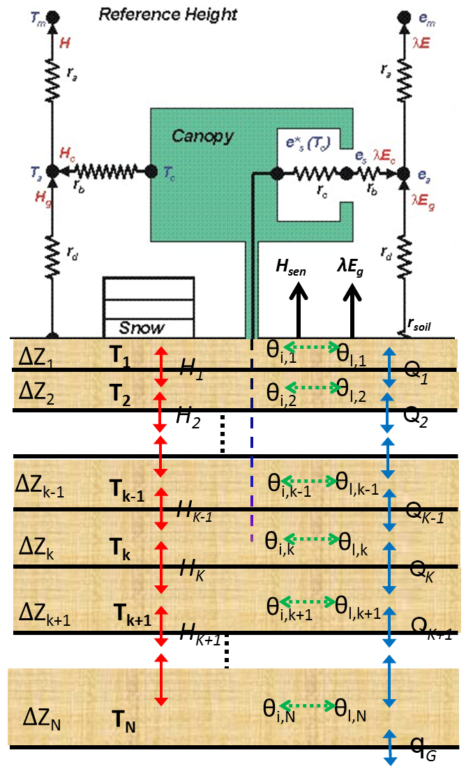
Figure 1Schematic diagram of SSiB3-FSM. Soil temperature, soil volumetric water content and soil volumetric ice content are T, θl and θi, respectively. The heat and water flux between soil layers are represented by Hk and Qk. The soil layer number is k, which ranges from 1 to N.
The soil column is discretized into 8, 11 and 12 layers for desert, grassland and trees, respectively. The thickness of each soil layer increases with the soil depth, and the depths of the soil column vary with vegetation types in SSiB3. The deepest soil depth also depends on the upper vegetation type. For example, the deepest soil depth over bare soil and grassland is 7.77 m, and over forest it is about 12 m. The surface soil layer was assigned as 2 cm since the variables in the surface are sensitive to the atmospheric diurnal forcing.
2.2.1 Energy balance equations
The energy balance equation for the canopy indicates that the canopy energy storage change with time is affected by the net radiation at the canopy layer and can be written as
The heat budget of the uppermost soil layer is affected by the net radiation at the soil surface (Rngs; W m−2), sensible heat (Hgs; W m−2), latent heat fluxes (λEgs; W m−2), energy exchange with lower soil layer and the phase change between ice and liquid and can be written as
The energy distribution inside the soil column is controlled by the heat conduction between layers and the phase change inside each individual layer, so it can be written as
The first term of Eq. (3) on the left is the heat storage change with time in each soil layer. The second term is the latent heat due to freezing–thawing. The first term on the right is the convective heat transferred between the soil layers. At the bottom boundary layer, it is assumed that there is no heat flux from the deeper soil. The differences of energy balance equations for soil between SSiB3 and SSiB3-FSM are the phase change between ice and liquid in the SSiB3-FSM and directly use the heat conduction equation rather than the force-restore method.
2.2.2 Water balance equations in soil layers
The water distribution within the soil is driven by the liquid water movement and liquid–ice phase change. This scheme treats the freeze–thaw process as continuous, without a fixed freezing point, and allows the coexistence of water and ice to modify the hydraulic and thermal properties of the soil. The conservation of liquid flow is expressed as a one-dimensional Richards' equation:
The liquid water flow rate of Ql (m s−1) is described by Darcy's law (see Eq. B5 in Appendix B). In the SSiB3-FSM, a freeze–thaw process scheme is used, which is derived from the freezing point depression and soil water potential curve in frozen soil:
This equation has been employed to describe the relationships among soil temperature, soil liquid water content, and ice content (Li et al., 2010).
2.2.3 Numerical scheme for the thermal and hydrological equations
Equations (1)–(5) are highly nonlinear systems because the ice content and liquid water change rapidly with little soil temperature change during soil freezing or thawing. We previously substituted soil enthalpy and total water mass for soil temperature and volumetric liquid water content in governing equations (Li et al., 2010) to solve highly nonlinear differential equations. This method also retains energy and water conservation and represents the continuous and slow energy change in the frozen soil system during the freezing–thawing process. However, this approach was only tested for limited field sites. While the method was used in the coupled SSiB3-FSM and tested over a global domain, the numerical solutions become unstable during the long-term integrations for some grid points because the global soil properties and meteorological forcing vary widely. Therefore, a semi-implicit solution procedure for the soil energy and water prognostic equations was developed with SSiB3-FSM for this study.
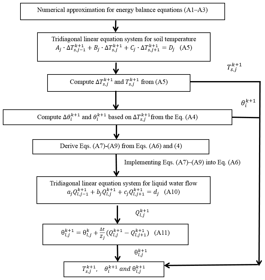
Figure 2 presents a flowchart of the semi-implicit solution procedure for SSiB3-FSM. A semi-implicit backward finite-difference approximation was used for the thermal diffusion equations for canopy and soil (Eqs. 1–3). The numerical Eqs. (B1)–(B3) are shown in Appendix B. Meanwhile, Eq. (5) was transformed to a numerical form (B4) so that it can represent the relationship between the change in soil temperature (ΔTs) and the change in soil ice content (Δθi) assuming the total water mass is conserved during one time step. Then a tridiagonal linear equation system (B5) for the change in soil temperature was derived based on Eqs. (B1)–(B3), (B4). After solving the tridiagonal matrix at different soil layers, the phase change between liquid water and ice (Δθi) in soil was decided using the change in soil temperature (ΔTs) during one time step (Eq. B4). Because the phase change has been included while solving the temperature tridiagonal matrix, here we obtained the soil water content (θi) and soil temperature (Ts) for each soil layer. After the change in ice content has been decided, the water balance equations do not involve the prognostic variable of the ice content. Subsequently, we can solve the tridiagonal matrix for water fluxes at the interface of the soil layers (see Appendix B, Eqs. B6–B10). The liquid water content at the current time step can be easily obtained from Eq. (B11).
This semi-implicit scheme for soil temperature, liquid water and ice content in SSiB3-FSM has been tested over the global domain. Compared to the previous method that substituted soil enthalpy and total water mass for soil temperature and volumetric liquid water content, this coupling scheme can effectively produce stable solutions for at least 60 years of integrations with the heat and mass balances.
3.1 Data sets
From 1948 to 2007, the SSiB3 model and coupled offline SSiB3-FSM model were driven using the meteorological forcing from the Princeton global meteorological forcing data set (Sheffield et al., 2006), which is developed by combining a suite of global observation-based data sets with the National Centers for Environmental Prediction/National Center for Atmospheric Research reanalysis data. The data set includes surface air temperature, pressure, specific humidity, wind speed, downward short-wave radiation flux, downward long-wave radiation flux and precipitation. The spatial resolution is 1∘ × 1∘, and the temporal resolution is 3 h.
Several observation data sets have been used to evaluate the performance of SSiB3-FSM and SSiB3 in cold regions. For the surface skin temperature (Tgs), we used the Global Historical Climatology Network version 2 and the Climate Anomaly Monitoring System (GHCN-CAMS) gauge-based 2 m temperature over land for 1979–2007, which provides global coverage of monthly means at a regular resolution of 0.5∘ latitude × 0.5∘ longitude grids (Fan and van den Dool, 2008). Although GHCN-CAMS data are air temperature data, in fact the changes in 2 m air temperature are highly consistent with those in skin temperature. Therefore, GHCN-CAMS air temperature data were used to validate the simulated land surface skin temperature globally.
For the soil temperature profile and the MFD over the TP and NC, the monthly mean soil temperature of 626 stations over China for 1981–2005 has been used (Yang and Zhang, 2016), provided by the China Meteorological Administration (2008). The data set has nine soil layers at 0, 5, 10, 15, 20, 40, 80, 160 and 320 cm.
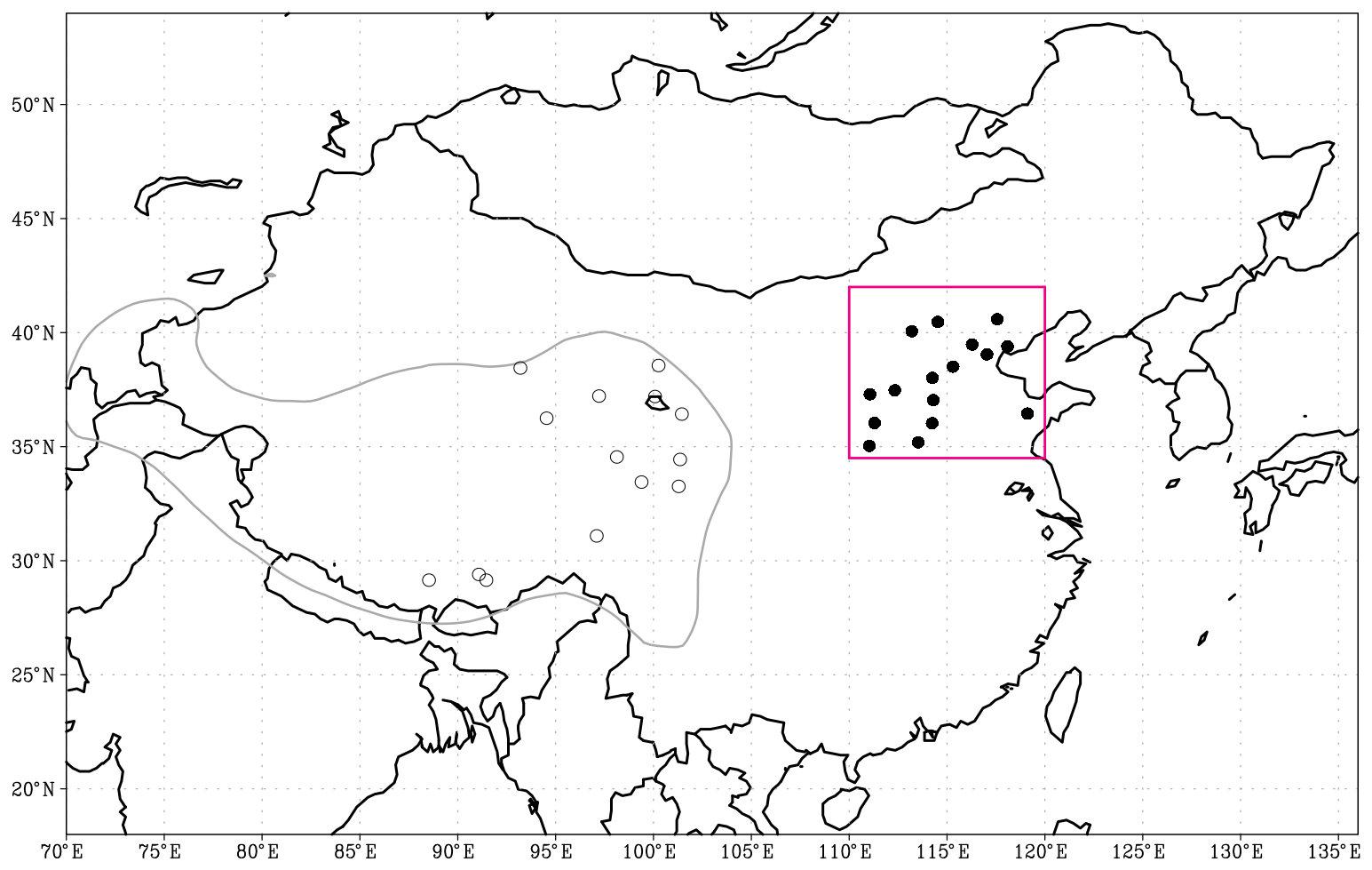
Figure 3Geographical distribution of stations with complete soil temperature records for all nine soil layers for 1981–2005. The red boxed region is North China (110–120∘ E, 34.5–42∘ N), and the locations of the 16 sites used in this study are marked by solid circles. The grey line shows that the elevation is above 2500 m, and the grey empty circles denote the locations of the 14 sites on the TP.
Since the calculation of land soil temperature memory requires a long time series of soil temperature data, only the stations with complete records for 1981–2005 and nine soil layers over the TP region (elevation > 2500 m) and NC (110–120∘ E, 34.5–42∘ N) were selected. There are 14 stations over the TP and 16 sites over NC used for this study. Figure 3 shows the spatial distribution of the stations with available soil temperature data for all nine soil layers and for all 12 months of all 25 years over the TP and NC.
3.2 Experimental design and methods
3.2.1 Control run
A global simulation by SSiB3-FSM and SSiB3 was carried out forced by the Princeton global meteorological forcing data set from 1948 to 2007. The initial soil temperature and liquid water content profiles were derived by interpolating the NCEP-DOE Reanalysis II (R2) (NCEP-R2, Kanamitsu et al., 2002) soil temperature and soil moisture data linearly to the model's soil layers. Because the soil ice content measurements are unavailable and the initial soil ice content is essential for the soil hydrological and thermal properties, we set ice content to zero at the beginning. The first 10 years (1948–1957) were used for model spinup, and the simulation for the last 50 years (1958–2007) was analyzed. The observational data were used to evaluate the model performance, and the results from this run were used to analyze the cold regions' thermal characteristics and MFD as well as their variations under global warming.
3.2.2 Sensitivity run
To investigate the sensitivity of the soil temperature profile and other thermal characteristics to the freeze–thaw process, we conducted a sensitivity simulation using the SSiB3-FSM under the same initial land surface conditions but without the freeze–thaw process in soil. This sensitivity run is referred to as the SSiB3-FSMnoICE run hereafter. Both the SSiB3-FSM run and the SSiB3-FSMnoICE run produce multi-layer soil temperature and soil moisture, MFD, net radiation, latent heat flux and sensible heat flux as well as the canopy temperature, canopy water and interception.
3.2.3 Methodology to determine MFD and soil memory
Based on the classification of the permafrost by Frauenfeld et al. (2004), a site was deemed to be seasonally frozen ground while the soil temperature at 3.2 m is above 0 ∘C. Based on this criterion, the 14 stations over the TP and the 16 sites over NC in this study were all classified as seasonally frozen ground. According to the seasonal characteristic of soil temperature over seasonally frozen ground, the MFD for each year can be defined as an index for the study of seasonal frozen soil variability and change. This paper gives a preliminary estimation of MFD variations based on monthly soil temperature. Following Frauenfeld et al. (2004), the maximum depth of the zero isothermal line for some year is defined as the MFD for this year. Frauenfeld et al. (2004) validated this robustness of this approach. It should be noted that the MFD is different from active layer thickness (ALT) because the active layer is defined as “the top layer of ground subject to annual thawing and freezing in areas underlain by permafrost” (van Everdingen, 1998). ALT is suitable for the permafrost, but MFD is more suitable for the seasonally frozen ground. As the ALT increases, the permafrost thaws deeper, whereas as the MFD increases, the frozen soil freezes deeper.
The persistence of soil temperature can be quantified by temporal scale analysis. Hu and Feng (2004) assumed that the temporal variation of the soil enthalpy in North America followed the first-order Markov process. Instead of analyzing soil temperature only, the variation of soil enthalpy, which represents integration of soil temperature through the soil column, was used to examine the land memory (Hu and Feng, 2004). This study uses the observed and simulated soil temperature from ground stations in NC and the TP and the method presented in Entin et al. (2000) and Hu and Feng (2004) to analyze the persistence. Land memory is characterized by the variable's autocorrelation, r, satisfying the following:
in which δt is the time lag, S is the decay timescale that can characterize a red noise process and r(δt) is the autocorrelation coefficient at the lag time (e.g., 1, 2, 3 months, ... ).
4.1 Assessment of simulated surface 2 m temperature and temperature profile
4.1.1 Surface 2 m temperature
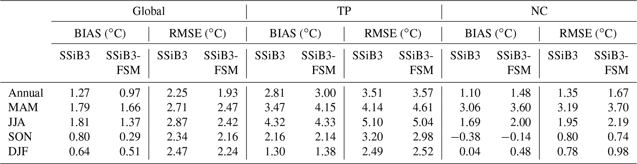
Before investigating the frozen soil thermal characteristics and MFD as well as their variability, the SSiB-FSM is first evaluated using the observational data. The root mean square error (RMSE) and absolute bias (BIAS) between CAMS and simulated surface temperature globally as well as TP and NC from the SSiB3-FSM and SSiB3 are assessed (Table 1). Table 1 shows that the annual RMSE and BIAS of SSiB3-FSM are less than those of SSiB3. In addition, in different seasons the SSiB3-FSM shows less bias than SSiB3. Overall, the SSiB3-FSM produces more realistic estimates of surface temperature than SSiB3, and it can predict the heat transfer processes globally and locally with a reliable accuracy, which provides a basis for further discussions.
Table 1Error statistics of the simulated surface temperature by SSiB3-FSM and SSiB3.
4.1.2 Soil temperature profile in the TP
The seasonal vertical soil temperature profile strongly mirrors the influence of the air temperature forcing, in contrast to the almost isothermal average annual temperature profile (Oelke and Zhang, 2004). The averaged seasonal profiles for observed soil temperature at 14 sites over the TP are shown in Fig. 4a. For easy comparison, only soil temperature profiles in January, April, July and October are shown, since the four curves represent the characteristics of the soil temperature profile in winter, spring, summer and fall, respectively. At the seasonal scale, the surface layer and the subsurface layers (here referred to the surface to ∼ 1 m) are frozen during winter (January), whereas the temperature of the deep layers (below 1 m) is above 0 ∘C. The surface and subsurface soil begins to thaw from March. In April the soil is almost unfrozen. Deep soil temperature always stays above 0 ∘C.
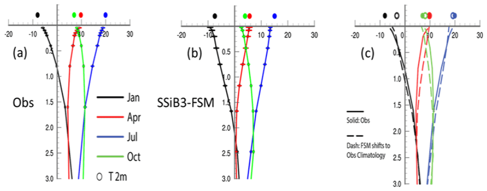
Figure 4The seasonal soil temperature profile over the TP (14 sites) for 1981–2005. (a) Observation; (b) simulated by SSiB3-FSM; (c) comparison between the observation and the SSiB3-FSM shifts to the observation climatology.
There is a generally rising trend in monthly temperature from winter to summer (from January to July) above 2 m soil depth. Between the 2 and 2.5 m depths there are no apparent changes in soil temperature from January to April. Below 2.5 m, there is an inverse trend compared with upper soil temperature. For instance, the temperature in January is higher than that in April at 3 m soil depth. From April to July, the temperature of all soil layers (surface to ∼ 3.2 m) increases with the air temperature due to the increasing solar radiation. As the fall approaches, the soil temperature above 1.5 m begins to decrease. Below 1.5 m there is a time lag behind the rising trend, leading to higher temperature at 3.2 m in October than that in July. From October to January, soil temperature in all layers shows a decreasing trend. Generally, the soil is characterized as seasonally frozen ground. Deep soil temperature shows a time lag compared with the surface layer, and the upper soil temperature (< 1.5 m) shows larger seasonal variability than the deep soil temperature.
The simulated soil temperature profile by SSiB3-FSM over the TP in different seasons is shown in Fig. 4b. There is a general consistency between the simulated temperature profile and the observed profile in both vertical distribution and the seasonal variations. Compared against observations, however, the simulated soil temperatures underestimate the temperature in the whole soil column throughout all seasons. The air temperature at 2 m in April, July and October in SSiB3-FSM is lower than that observed. This systematic bias arises from the forcing data. For example, the observed air temperature in April at 2 m is about 10 ∘C, but the forcing for the models is only 6 ∘C. The greatest difference (about 6 ∘C) is in July. Considering the forcing data's bias, we can in parallel move the SSiB3-FSM soil temperature profile to put the simulated and observed 2 m temperature climatologies in the same position. Subsequently, the observed and simulated soil temperature profiles almost coincided (Fig. 4c).
4.1.3 Soil temperature profile in NC
The simulated and observed seasonal soil temperature profiles over NC are displayed in Fig. 5a and b, respectively. They show a similar seasonal frozen soil temperature variability to those over the TP, but its thawing season is earlier than that of the TP. As the observations show, in winter (January), the soil freezes above 40 cm, and it begins to thaw in February until March. The soil under 40 cm stays above 0 ∘C throughout the year. The simulated temperature profiles and their seasonal variations are adequately consistent with the observations. However, the frozen depth is deeper in SSiB3-FSM than that of the observations in January (Fig. 5c). These differences may be attributed to the parameterization of soil thermal and hydrological processes in SSiB3-FSM.
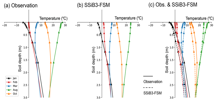
Figure 5The seasonal soil temperature profile over NC (16 sites) for 1981–2005. (a) Observation; (b) simulated by SSiB3-FSM; (c) observation and SSiB3-FSM.
4.1.4 Comparison with the force-restore method
In SSiB3 with the force-restore method, only surface temperature and deep soil temperature are considered. For the seasonal change in soil temperature, both the seasonal variation of surface soil temperature (Tgs) and deep soil temperature (Td) (Fig. 6a and c) are on the same phase, only with a weak lag in Td. It is difficult to define its precise position of the deep soil temperature layer, which is dependent on the vegetation types and soil conditions. By introducing a multi-layer frozen soil model, SSiB3-FSM not only presents more precise soil temperature profile, but also clearly shows the seasonal change in soil temperature at different soil depths (Fig. 6b and d). The time lag and amplitude damping of temperature become more pronounced with increasing depth, and they are well described in SSiB3-FSM (Fig. 6b and d). This improved performance of SSiB3-FSM lays a foundation for further investigation of the characteristics of MFD changes and soil memory.
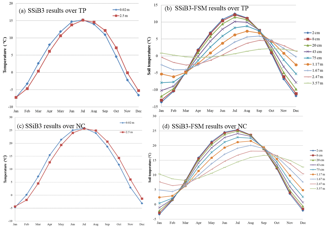
Figure 6The seasonal soil temperature simulated by SSiB3 and SSiB-FSM over the TP (14 sites) and NC (16 sites) for 1981–2005. (a) The seasonal climatology of Tgs (0.02 m) and Td (2.5 m) by SSiB3 over the TP; (b) the seasonal temperature climatology by SSiB3-FSM over the TP; (c) the seasonal climatology of Tgs (0.02 m) and Td (2.5 m) by SSiB3 over NC, and (d) the seasonal temperature climatology by SSiB3-FSM over NC.
4.2 Characteristics of the soil temperature profile over the TP and NC
4.2.1 Temporal variability of the soil temperature profile over the TP and NC
The temporal variability with depth of soil temperature was further explored by analyzing the phase variations with depth. Here, we used the cross-correlation statistical method to analyze how the seasonal variability in soil temperature decreases with depth. Because the SSiB3-FSM produced reasonable surface and subsurface temperature profiles (as discussed in Sect. 4.1) and the observational data are only at monthly resolution, the 50-year simulated daily soil temperatures were used to represent the time–space variability of soil temperature over a wide area. Figures 7a and 8a show the lag cross-correlations between soil temperature of the first layer with other layers over the TP and NC, respectively. The time lag at which the maximal correlations occur increases with soil depth. For instance, the soil layer at 59 cm reaches maximum at about 10 d, while the layer at 312 cm needs about 90 d (a season). The cross-correlation values decrease after they reach the maximum value and reach zero at about 110 and 180 d for the soil layer at 59 and 312 cm, respectively. The soil temperature phase lag time was used to more clearly display these relationships. It is defined as the point at which the cross-correlation with the first soil layer equals 1 (in Figs. 7a and 8a). The change in soil temperature phase lag time with soil depth is shown in Figs. 7b and 8b. The phase lag time increases linearly with the soil depth, the details of which are presented in Table 2. For the soil depth at 1.5 m over the TP, the phase lag for soil temperature is about 43 d (∼ 1.5 months). For the soil depth at 3 m, the phase lag could be 87 d (∼ 3 months). Over NC, the phase lag for soil temperature is 11 and 32 d at 59 cm and 1.5 m, respectively.
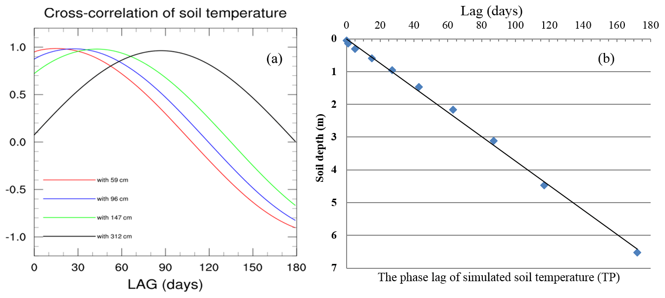
Figure 7The time–space variability of soil temperature over the TP for 1978–2007. (a) Simulated cross-correlation of the first-layer soil temperature with other soil layers (red line: 59 cm; purple line: 96 cm; green line: 147 cm; black line: 312 cm) by SSiB3-FSM; (b) the phase lag (days) of simulated temperature over the TP by SSiB3-FSM.
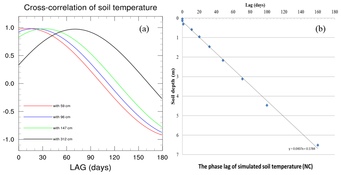
Figure 8The time–space variability of soil temperature over NC for 1978–2007. (a) Simulated cross-correlation of the first-layer soil temperature with other soil layers (red line: 59 cm; purple line: 96 cm; green line: 147 cm; black line: 312 cm) by SSiB3-FSM; (b) the phase lag (days) of simulated temperature over NC by SSiB3-FSM.
Table 2Phase lag (days) of simulated soil temperature at different soil depths by SSiB3-FSM and SSiB-FSMnoICE.

4.2.2 Land memory
The land surface temperature anomaly over the TP and North America has been recognized as an indicator of extreme hydroclimate events (Xue et al., 2018) because of its preservation of the snow and other climate signatures in previous months. Evaluating the soil persistence of SSiB3 and SSiB3-FSM and comparison with observed soil memory are crucial for its application in climate studies. The above analysis of temporal variability in soil temperature with depth shows that the soil temperature simulated by SSiB3-FSM is characterized by increasing persistence with depth. This suggests SSiB3-FSM can be used to study the land persistence of soil enthalpy, which represents integration of soil temperature through the soil column.
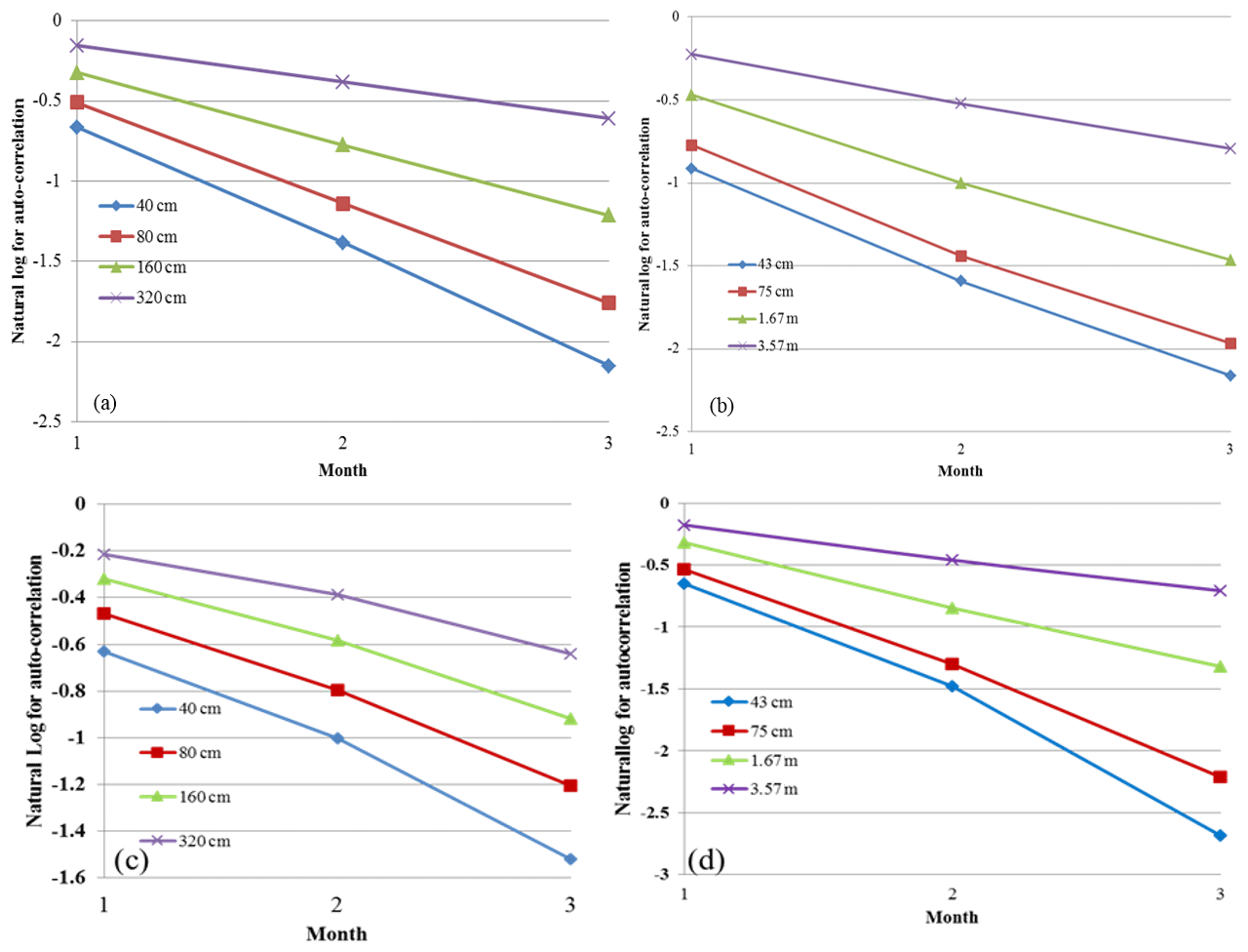
Figure 9The natural log for the auto-correlation over NC (a, b) and the TP (c, d) for 1981–2005. (a, c) Observed; (b, d) SSiB3-FSM.
Taking the natural log on both sides of Eq. (6) and rearranging, we can obtain , which describes a straight line in the two-dimensional domain of δt and the natural log of autocorrelation, r. Following this procedure, we calculated autocorrelations of observed monthly soil enthalpy anomalies between 5 and 320 cm at time lags from 1 to 4 months at the 16 stations over NC and 14 sites over the TP and plotted their average autocorrelations in the δt−ln [r(δt)] domain (Fig. 9a and c). The lagged autocorrelations of the simulated monthly soil enthalpy anomalies at different soil layers between 5 and 312 cm were also calculated and are shown in Fig. 9b and d. The persistence of soil enthalpy anomalies is determined by the negative inverse of the slope of the straight line for each case in Fig. 9. The slope of these lines varies, indicating a different persistence time of the soil enthalpy anomaly at different depths.
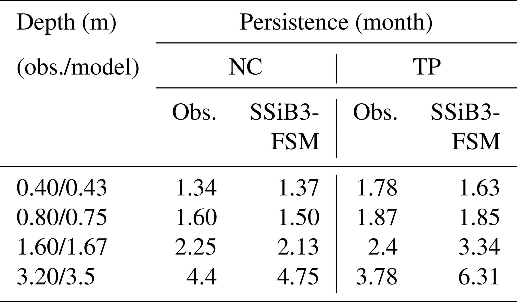
The persistence values over NC and the TP are given in Table 3. For the observations over NC, the persistence of soil enthalpy anomalies is about 1.34 months in the top 40 cm column and increases to longer than 2 months in the top 160 cm column under the soil surface. In the 320 cm soil column the persistence of soil enthalpy anomalies reaches 4.4 months. Similarly, the persistence of simulated soil enthalpy anomalies is 1.37 months in the 43 cm below the surface. It increases to longer than 2 months about the 167 cm soil column. For the TP, as with NC, both the observed and simulated soil persistence gradually increase with soil depths. The simulated soil persistence below 1.60 m over the TP is larger than the observed one. We will explore the difference in the next study. Generally, over both the TP and NC the observed persistence change with the soil thickness is reasonably simulated with the SSiB3-FSM.
Table 3The persistence of soil temperature at different soil depths over the TP and NC by SSiB3-FSM and the observations.
The persistence by SSiB3 with the force-restore method over the TP is only 1.2 and 1.23 months for the surface temperature and deep temperature, respectively. For NC, the results by SSiB3 are also about 1 month for the surface temperature and deep temperature. SSiB3-FSM shows better performance in simulating the land persistence for the anomalies in soil than SSiB3, which only considers two layers of temperature data.
4.3 Sensitivity of the soil temperature profile to the freeze–thaw process
A sensitivity experiment, test-SSiB3-FSMnoICE, in which the freeze–thaw process in soil is not included, was detailed in Sect. 3.2.2. A comparison of soil temperature profiles was made between SSiB3-FSM and SSiB3-FSMnoICE, and the results are shown in Fig. 10. With freeze–thaw parameterization, the latent heat released while freezing, e.g., in October, could offset the decreasing soil temperature. The soil temperature, therefore, would be higher than that of SSiB3-FSMnoICE. Over the TP, the largest difference is found for January, especially between 50 cm and 1.5 m. The simulated soil temperature by SSiB3-FSM is about 1–1.7 ∘C higher than that by SSiB3-FSMnoICE. Over NC, the large differences are also shown in winter, especially in January. The difference in January is about 1–1.2 ∘C from 15 cm to 1.5 m, which means the freeze process in soil delays the winter cooling in freezing seasons (from October to January) and delays the summer warming in thawing seasons (from April to July).
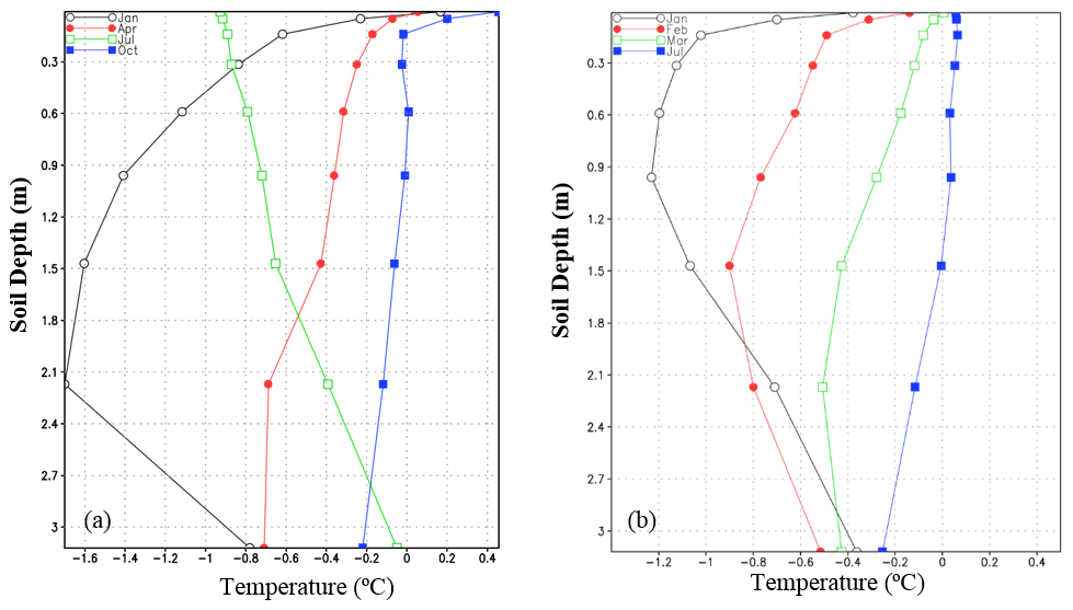
Figure 10Differences in the seasonal soil temperature profile between the SSiB3-FSMnoICE and SSiB3-FSM for 1981–2005 over (a) the TP (14 sites) and (b) NC (16 sites).
The freeze–thaw process has a major impact on soil temperature profile simulation, especially when freezing or thawing occurs. This effect would exert an impact on the spatial and temporal variability of soil temperature and play an essential role in the soil temperature time lag. Table 2 shows that the time lag of SSiB3-FSMnoICE is less than that of SSiB3-FSM in almost every soil layer. In particular, over the TP, the difference of lag days between the SSiB3-FSM scheme and SSiB3-FSMnoICE scheme increases with depth. For instance, at 59 cm, the time lag of the SSiB3-FSM scheme is 3 d longer than that of the SSiB3-FSMnoICE scheme; however, at about 3 m depth, the difference is about 15 d. For NC, the freeze–thaw processes also increase the phase lag days even though the number of phase lag days between the SSiB3-FSM and SSiB3-FSMnoICE show less difference than those over the TP in the upper soil depths. This is because the maximum freezing depth over NC is about 30 cm, much shallower than that over the TP. Correspondingly, the effects of the freeze–thaw process are only exerted at shallower soil depths.
4.4 MFD over the TP
The long-term temperature profiles at 14 stations over the TP and 16 sites over NC exhibit characteristics of seasonally frozen ground, which freezes in winter and thaws in spring at the surface soil and remains unfrozen at 3.2 m depth throughout the entire year. The simulated annual soil temporal variations with soil depth over the TP and NC stations are shown in Fig. 11, which displays the seasonal freezing and thawing processes during 1981–2005 for the TP and NC. Over the TP, the surface soil starts to freeze in the middle of October and the MFD occurs around April at 1.8 m. For NC, the surface soil starts to freeze at the beginning of December and the MFD occurs in February at around 60 cm soil depth, which is much shallower than that of the TP.
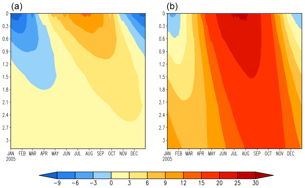
Figure 11The climatology of simulated daily soil temperature (a) over the TP (14 sites averaged) and (b) NC (16 sites averaged) for 1981–2005 (unit: ∘C).
The MFD at 14 sites over the TP and 16 sites over NC simulated by SSiB3-FSM was averaged to analyze the changes in the MFD for 1981–2005. As for the simulated MFD, it shows large difference from the observational MFD. This difference of MFD between simulation and observation comes from the systematic bias of forcing data, just shown in Figs. 4 and 5. Therefore, zero-score normalization, which is a commonly used normalization method, was employed to normalize the observed and simulated MFD:
where xi is the original MFD value for 1981–2005 and yi is the normalized MFD corresponding to xi.
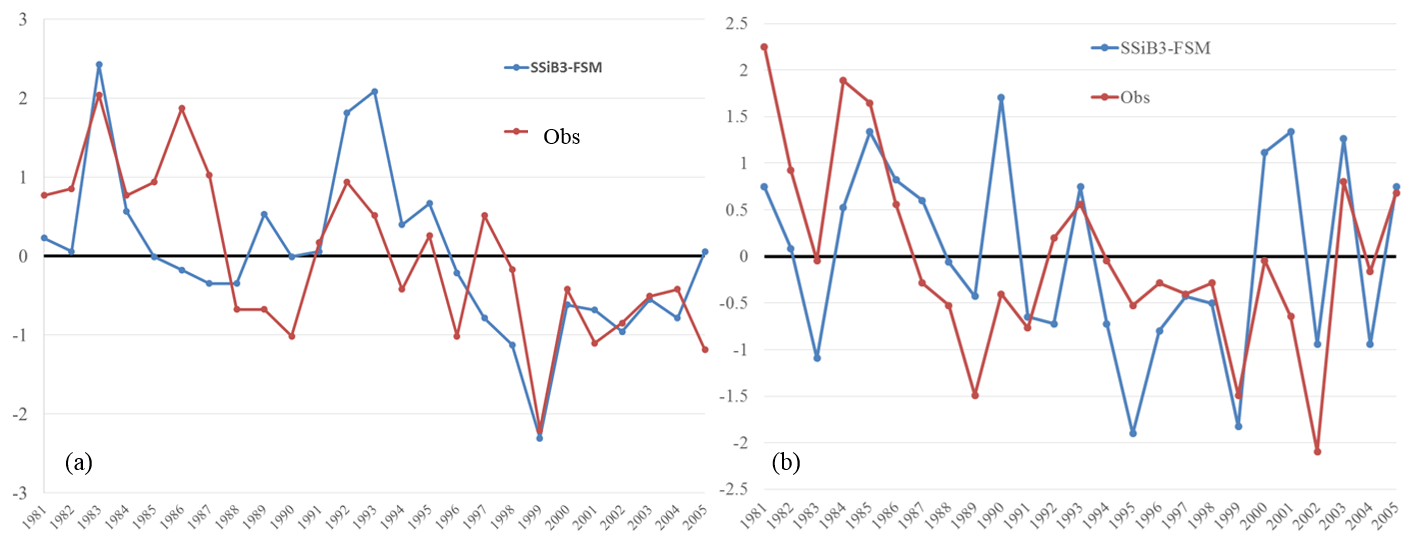
Figure 12Normalization of MFD over (a) the TP and (b) NC for 1981–2005 for SSiB3-FSM and the observations.
Both the observed MFD over the TP and NC showed a significant decreasing trend from 1981 to 2005 (Fig. 12). These decreasing trends indicate that, in areas of seasonally frozen ground, the freezing ground became increasingly shallower during this time period. Over the TP, the observed net change is a 23 cm decrease in MFD in 2005 compared with 1981, and the rate of decrease is about 0.92 cm yr−1. However, from 1983 to 1990 the rate is about 4.5 cm yr−1, which is about 4 times as much as that in 1981–2005. In the 1990s, the decreasing rate is about 3 cm yr−1. After the 2000s, the decreasing trend reduced. A similar decrease in the simulated normalized deviation of MFD at 14 TP sites for 1981–2005 is shown in Fig. 12a. The rate of decrease intensified during 1983–1990, which was also shown in the observations.
Over NC, the observed decrease in MFD is 13 cm from 1981 to 2005. The highest decreasing rate is about 3.1 cm yr−1 from 1981 to 1990, about 6 times higher than in 1981–2005. The simulated results by SSiB3-FSM also show the consistency with the observations, especially during the 1980s, when the MFD decreasing trend is 1.8 cm yr−1.
The MFD decreasing trend during the 1980s over the TP may be related to the significant increasing trend in the winter and spring air temperature. Wei et al. (2003) analyzed the inter-decadal variations of air temperature over the TP and found a global climatic jump in the 1980s on the TP, and the air temperature increased more strongly in the winter and spring from the 1980s to 2000s. They showed that the rates of increasing air temperature at most stations were 0.02–0.04 ∘C yr−1 in the winter and spring, which leads to an increasing trend in the 10–20 cm soil temperature over the TP (Zhang et al., 2008). For NC, an increasing winter temperature trend has been detected since 1985 (Zhang et al., 2002; Shen et al., 2010), which may lead to the decreasing MFD over NC since the 1980s.
It can be seen that the decreasing trend of MFD stabilized after 2000. Because MFD was mainly controlled by the winter surface temperature. Spatio-temporal analysis of surface temperature over the TP during 1981–2015 shows that the winter surface temperature over the TP increased significantly in the 1980s, and the temperature changes were relatively stable in the 1990s and early 21st century (Bai et al., 2018). That is why the decreasing trend of MFD over the TP after 2000 is stabilized.
A comparison of MFD between SSiB3-FSM and SSiB3-FSMnoICE was conducted to evaluate the effects of freeze–thaw processes on the MFD. Although the heat and water mass balance due to ice–liquid phase change is not included in SSiB3-FSMnoICE, the soil temperature still experiences a large range of variation. Both MFDs show almost the same variations, but the MFD in SSiB3-FSM is shallower than that in SSiB3-FSMnoICE (figure not presented). This can be explained by the phase change energy released while freezing, which could offset the decreasing temperature during the freezing period and lead to a higher soil temperature at the same soil depth than that simulated by the SSiB3-FSMnoICE.
To improve the accuracy of soil temperature simulation in frozen ground, a multi-layer FSM was incorporated into SSiB3 to represent the freezing–thawing process and the heat and water transfer in a multi-layer frozen soil. By introducing a semi-implicit backward finite-difference approximation and a freezing–thawing scheme based on the freezing depression equation, the highly nonlinear equations in multi-layer frozen soil can be efficiently and stably solved by two tridiagonal matrixes in SSiB3-FSM. The simulated results show that with the frozen soil component, the SSiB3-FSM produces realistic soil thermal characteristics than that of SSiB3, especially soil vertical temperature profiles in different seasons.
Furthermore, our results confirm the important role of frozen soil processes in soil thermal characteristics at different timescales over NC and the TP. The results show that the phase-change latent heat released while freezing can offset the decreasing soil temperature; therefore, the soil temperature could be higher than that of the experiment without the frozen soil process as soil freezes. Further analysis of the spatial and temporal variability of soil temperature showed that the seasonal variability of soil temperature decreases with soil depths, and the phase lag damps linearly. The frozen soil process could increase the phase lag of soil temperature from several days in the surface layer to 15 d in deep layers.
The investigation of SSiB3-FSM's ability to simulate the variability of maximum frozen depth at decadal scales showed that simulated normalized MFDs over the TP and NC by SSiB3-FSM are in good agreement with the observations for 1981–2005, including the substantial decreasing trends and the variabilities at decadal scales. The frozen soil processes affect the magnitudes but do not change the decreasing trends of MFD. SSiB3-FSM shows shallower MFD than SSiB3-FSMnoICE because the simulated soil temperature in SSiB3-FSM is higher than that in SSiB3-FSMnoICE. In addition, the SSiB3-FSM also can reproduce the reliable soil memory at different soil depths.
The changes in soil properties and their parameterizations have great effects on the surface energy balance. In particular, the soil thermal conductivity shows large spatial variabilities, and the soil thermal properties are heterogeneous in the vertical direction. A disparity of the soil properties between models and observations may result in the difference between the observations and the simulations.
Although the SSiB3-FSM is capable of capturing the basic soil thermal characteristics at seasonal and decadal scales over regions of seasonally frozen ground, further analyses into soil hydrological characteristics in the freezing and thawing phases remain to be conducted. In addition, the better performance of SSiB3-FSM than that by SSiB3 or SSiB3-FSMnoICE is not only attributed to the frozen soil process, but also to the multi-layer heat and water transfer scheme. The effects of the soil stratification and the soil column depth on the model's performance over seasonal frozen ground require further study.

In SSiB3-FSM, a semi-implicit backward finite-difference approximation was used for the thermal diffusion in the soil.
For energy balance equation at canopy layer, Eq. (1) can be written as
where ΔTc and ΔTgs denote the change in Tc and Tgs during a time step.
For groundcover and soil, Eq. (2) can be written as
For the inner layer, Eq. (3) can be written as
Assuming the total water mass is conserved during one time step, the change in soil temperature (ΔTs) and the change in soil ice content (Δθi) can be derived based on Eq. (5):
Inserting Eq. (5) into Eqs. (B1)–(B3), the energy balance equation system can be reorganized as a tridiagonal linear equation system with soil temperature of all the soil layers:
where Aj, Bj and Cj are the known coefficients and functions of , Ts,j and at the previous time step. Dj also represents the known values at the previous time.
After solving the tridiagonal matrix for the soil temperature change at different soil layers, we can obtain the soil temperature at the current time step (Ts,j). In addition, the phase change between liquid water and ice in soil can be decided using the change in soil temperature during one time step. Because the phase change has been included while solving the temperature tridiagonal matrix, here we can obtain Δθi using Eq. (B4). Then we can solve the water fluxes at the interface of the soil layers:
Combining Eq. (B6) with Eq. (4), we can obtain water balance equations for the surface layer,
for the root zone layer,
and for the bottom soil layer,
Inserting Eqs. (B7)–(B9) into Eq. (B6) and then regrouping Eq. (B6), we obtain a tridiagonal linear system for liquid water flow as follows:
where aj, bj and dj are the known coefficients and functions of ψj, ψj+1 and θl,j, at the previous time step. Therefore, the water fluxes at the current time step can be solved using the above tridiagonal matrix. Then the liquid water content at the current time step can be easily obtained from the following equation:
The SSiB3-FSM code is available upon request from the first author. The analyses are developed within the Grads and Python software environment. The scripts are also available upon request from the first author. The CAMS gridded 2 m temperature is available at https://psl.noaa.gov/data/gridded/data.ghcncams.html (Fan and van den Dool, 2008). The Princeton global meteorological forcing data set is available at http://hydrology.princeton.edu/data.php (Sheffield et al., 2006). The China Ground Temperature Grid Dataset is available at https://data.cma.cn/data/cdcdetail/dataCode/SURF_CLI_CHN_MUL_MON.html (China Meteorological Administration, 2008).
QL conceived the study and developed the model. QL and YX developed the framework of the study. QL and YX analyzed all of the simulation results and wrote the paper. QL and YL drafted the figures. All the authors discussed the results and contributed to finalizing the paper.
The authors declare that they have no conflict of interest.
We thank the editor and the reviewers for their instructive and insightful comments, which helped to strengthen this paper.
This research has been supported by the External Cooperation Program of Bureau of International Cooperation, Chinese Academy of Sciences (grant no. 134111KYSB20200020), the National Key Research and Development Program of China (grant no. 2018YFC1505701) and the National Science Foundation of United States (grant no. AGS-1849654).
This paper was edited by Xing Yuan and reviewed by three anonymous referees.
Bai, L., Yao, Y. B., Lei, X. X., and Zhang, L.: Annual and seasonal variation characteristics of Surface temperature in the Tibetan Plateau in recent 40 years, Journal of Geomatics, 43, 15–18, 2018.
Bao, H., Koike, T., Yang, K., Wang, L., Shrestha, M., and Lawford, P.: Development of an enthalpy-based frozen soil model and its validation in a cold region in China, J. Geophys. Res.-Atmos., 121, 5259–5280, https://doi.org/10.1002/2015jd024451, 2016.
Bi, H., Ma, J., Zheng, W., and Zeng, J.: Comparison of soil moisture in GLDAS model simulations and in situ observations over the Tibetan Plateau, J. Geophys. Res.-Atmos., 121, 2658–2678, 2016.
Chen, Y., Yang, K., Zhou, D., Qin, J., and Guo, X.: Improving the Noah Land Surface Model in Arid Regions with an Appropriate Parameterization of the Thermal Roughness Length, J. Hydrometeorol., 11, 995–1006, https://doi.org/10.1175/2010jhm1185.1, 2010.
China Meteorological Administration: Dataset of monthly surface climatological data (1951–present) from 613 stations in China, available at: https://data.cma.cn/data/cdcdetail/dataCode/SURF_CLI_CHN_MUL_MON.html (last access: 3 January 2020), 2008.
Clapp, R. B. and Hornberger, G. M.: Empirical equations for some soil hydraulic properties, Water Resour. Res., 14, 601–604, https://doi.org/10.1029/WR014i004p00601, 1978.
Collins, M., Knutti, R., Arblaster, J., Dufresne, J. L., Fichefet, T., Friedlingstein, P., Gao, X., Gutowski, W. J., Johns, T., Krinner, G., Shongwe, M., Tebaldi, C., Weaver, A. J., and Wehner, M.: Long-term Climate Change: Projections, Com-mitments and Irreversibility, in: Climate Change 2013: The Physical Science Basis. Contribution of Working Group I to the Fifth Assessment Report of the Intergovernmental Panel on Climate Change, edited by: Stocker, T. F., Qin, D., Plattner, G.-K., Tignor, M., Allen, S. K., Boschung, J., Nauels, A., Xia, Y., Bex, V., and Midgley, P. M., Cambridge University Press, Cambridge, UK and New York, NY, USA, 1029–1136, 2013.
Cuo, L., Zhang, Y., Bohn, T. J., Zhao, L., Li, J., Liu, Q., and Zhou, B.: Frozen soil degradation and its effects on surface hydrology in the northern Tibetan Plateau, J. Geophys. Res.-Atmos., 120, 8276–8298, https://doi.org/10.1002/2015jd023193, 2015.
Deardorff, J. W.: Parameterization of the Planetary Boundary layer for Use in General Circulation Models, Mon. Weather Rev., 100, 93–106, 1972.
Entin, J. K., Robock, A., Vinnikov, K. Y., Hollinger, S. E., Liu, S. X., and Namkhai, A.: Temporal and spatial scales of observed soil moisture variations in the extratropics, J. Geophys. Res.-Atmos., 105, 11865–11877, https://doi.org/10.1029/2000jd900051, 2000.
Fan, Y. and van den Dool, H.: A global monthly land surface air temperature analysis for 1948–present, J. Geophys. Res.-Atmos., 113, D01103, https://doi.org/10.1029/2007jd008470, 2008 (data available at: https://psl.noaa.gov/data/gridded/data.ghcncams.html, last access: 31 January 2021).
Fang, X., Luo, S., and Lyu, S.: Observed soil temperature trends associated with climate change in the Tibetan Plateau, 1960–2014, Theor. Appl. Climatol., 135, 169–181, https://doi.org/10.1007/s00704-017-2337-9, 2019.
Flerchinger, G. N. and Saxton, K. E.: Simultaneous heat and water model o f a freezing snow-residue-soil system: 1. Theory and development, Trans. ASAE, 32, 565–571, 1989.
Frauenfeld, O. W., Zhang, T. J., Barry, R. G., and Gilichinsky, D.: Interdecadal changes in seasonal freeze and thaw depths in Russia, J. Geophys. Res.-Atmos., 109, D05101, https://doi.org/10.1029/2003jd004245, 2004.
Guo, D. L. and Wang, H. J.: Simulation of permafrost and seasonally frozen ground conditions on the Tibetan Plateau, 1981–2010, J. Geophys. Res.-Atmos., 118, 5216–5230, 2013.
Guo, D. and Wang, H.: Simulated change in the near-surface soil freeze/thaw cycle on the Tibetan Plateau from 1981 to 2010, Chinese Sci. Bull., 59, 2439–2448, https://doi.org/10.1007/s11434-014-0347-x, 2014.
Guo, D. and Wang, H.: Simulated Historical (1901–2010) Changes in the Permafrost Extent and Active Layer Thickness in the Northern Hemisphere, J. Geophys. Res.-Atmos., 122, 12285–12295, 2017.
Hu, Q. and Feng, S.: A Role of the Soil Enthalpy in Land Memory, J. Climate, 3633–3643, https://doi.org/10.1175/1520-0442(2004)017<3633:AROTSE>2.0.CO;2, 2004.
Jin, R., Zhang, T., Li, X., Yang, X., and Ran, Y.: Mapping surface soil freeze-thaw cycles in China based on SMMR and SSM/I brightness temperatures from 1978 to 2008, Arct. Antarct. Alp. Res., 47, 213–229, https://doi.org/10.1657/aaar00c-13-304, 2015.
Kanamitsu, M., Ebisuzaki, W., Woollen, J., Yang, S.-K., Hnilo, J. J., Fiorino, M., and Potter, G. L.: NCEP-DOE AMIP-II Reanalysis (R-2), Bull. Am. Meteor. Soc., 83, 1631–1643, 2002.
Li, H., Wang, J., and Hao, X.: Influence of Blowing Snow on Snow Mass and Energy Exchanges in the Qilian Mountainous, Journal of Glaciology and Geocryology, 34, 1084–1090, 2012.
Li, Q., Sun, S., and Dai, Q.: The Numerical Scheme Development of a Simplified Frozen Soil Model, Adv. Atmos. Sci., 26, 940–950, 2009.
Li, Q., Sun, S., and Xue, Y.: Analyses and development of a hierarchy of frozen soil models for cold region study, J. Geophys. Res.-Atmos., 115, D03107, https://doi.org/10.1029/2009jd012530, 2010.
Li, X., Wu, T., Zhu, X., Jiang, Y., and Ying, X.: Improving the Noah-MP Model for Simulating Hydrothermal Regime of the Active Layer in the Permafrost Regions of the Qinghai-Tibet Plateau, J. Geophys. Res.-Atmos., 125, e2020JD032588, https://doi.org/10.1029/2020jd032588, 2020.
Liljedahl, A. K., Boike, J., Daanen, R. P., Fedorov, A. N., Frost, G. V., Grosse, G., Hinzman, L. D., Iijma, Y., Jorgenson, J. C., Matveyeva, N., Necsoiu, M., Raynolds, M. K., Romanovsky, V. E., Schulla, J., Tape, K. D., Walker, D. A., Wilson, C. J., Yabuki, H., and Zona, D.: Pan-Arctic ice-wedge degradation in warming permafrost and its influence on tundra hydrology, Nat. Geosci., 9, 312–318, 2016.
Liu, Y., Xue, Y., Li, Q., Lettenmaier, D., and Zhao, P.: Investigation of the Variability of Near-Surface Temperature Anomaly and Its Causes Over the Tibetan Plateau, J. Geophys. Res.-Atmos., 125, e2020JD032800, https://doi.org/10.1029/2020jd032800, 2020.
Luo, L. F., Robock, A., Vinnikov, K. Y., Schlosser, C. A., Slater, A. G., Boone, A., Braden, H., Cox, P., de Rosnay, P., Dickinson, R. E., Dai, Y. J., Duan, Q. Y., Etchevers, P., Henderson-Sellers, A., Gedney, N., Gusev, Y. M., Habets, F., Kim, J. W., Kowalczyk, E., Mitchell, K., Nasonova, O. N., Noilhan, J., Pitman, A. J., Schaake, J., Shmakin, A. B., Smirnova, T. G., Wetzel, P., Xue, Y. K., Yang, Z. L., and Zeng, Q. C.: Effects of frozen soil on soil temperature, spring infiltration, and runoff: Results from the PILPS 2(d) experiment at Valdai, Russia, J. Hydrometeorol., 4, 334–351, 2003.
Oelke, C. and Zhang, T.: A model study of circum-arctic soil temperatures, Permafrost Periglac., 15, 103–121, https://doi.org/10.1002/ppp.485, 2004.
Oelke, C. and Zhang, T.: Modeling the active-layer depth over the Tibetan plateau, Arct. Antarct. Alp. Res., 39, 714–722, 2007.
Poutou, E., Krinner, G., Genthon, C., and de Noblet-Ducoudré, N.: Role of soil freezing in future boreal climate change, Climate Dyn., 23, 621–639, https://doi.org/10.1007/s00382-004-0459-0, 2004.
Qin, D. H., Zhou, B. T., and Xiao, C. D.: Progress in studies of cryospheric changes and their impacts on climate of China, J. Meteorol. Res., 28, 732–746, 2014.
Sheffield, J., Goteti, G., and Wood, E. F.: Development of a 50-year high-resolution global dataset of meteorological forcings for land 50 surface modeling, J. Clim., 19, 3088–3111, https://doi.org/10.1175/jcli3790.1, 2006 (data available at: http://hydrology.princeton.edu/data.php, last access: 31 January 2021).
Shen, H. Y., Ding, Y. G., and Zhang, J.: Inter-decadal variations of winter air temperature in north China and its Circulation background, Scientia Meteorologica Sinica, 30, 338–343, https://doi.org/10.3969/j.issn.1009-0827.2010.03.008, 2010.
Slater, A. G., Bohn, T. J., Mc Creight, J. L., Serreze, M. C., and Lettenmaier, D. P.: A multimodel simulation of pan-Arctic hydrology, J. Geophys. Res.-Biogeo., 112, G04S45, https://doi.org/10.1029/2006jg000303, 2007.
Su, Z., de Rosnay, P., Wen, J., Wang, L., and Zeng, Y.: Evaluation of ECMWF's soil moisture analyses using observations on the Tibetan Plateau, J. Geophys. Res.-Atmos., 118, 5304–5318, https://doi.org/10.1002/jgrd.50468, 2013.
Sun, S.: Physical, Biochemical Mechanism of Land Surface Process and Its Parameterization, Meterol. Press, Beijing, China, 2005 (in Chinese).
Sun, S. and Xue, Y.: Implementing a new snow scheme in simplified simple biosphere model, Adv. Atmos. Sci., 18, 335–354, 2001.
Van Everdingen, R. (Ed.): Multi-language glossary of permafrost and related ground-ice terms (revised May 2005), National Snow and Ice Data Center, Boulder, USA, 1998.
Wei, Z. G., Huang, R., and Dong, W. J.: Interannual and Interdecadal Variations of Air Temperature and Precipitation over the Tibetan Plateau, Chinese Journal of Atmospheric Sciences, 27, 157–170, 2003.
Wu, Q. and Zhang, T.: Changes in active layer thickness over the Qinghai-Tibetan Plateau from 1995 to 2007, J. Geophys. Res.-Atmos., 115, D09107, https://doi.org/10.1029/2009jd012974, 2010.
Xue, Y., Sellers, P. J., Kinter, J. L., and Shukla, J.: A Simplified Biosphere Model for Global Climate Studies, J. Clim., 4, 345–364, 1991.
Xue, Y. K., Zeng, F. J., and Schlosser, C. A.: SSiB and its sensitivity to soil properties - A case study using HAPEX-Mobilhy data, Global Planet. Change, 13, 183–194, 1996.
Xue, Y. K., Sun, S. F., Kahan, D. S., and Jiao, Y. J.: Impact of parameterizations in snow physics and interface processes on the simulation of snow cover and runoff at several cold region sites, J. Geophys. Res.-Atmos., 108, 8859, https://doi.org/10.1029/2002jd003174, 2003.
Xue, Y., Diallo, I., Li, W., David Neelin, J., Chu, P. C., Vasic, R., Guo, W. D., Li, Q., Robinson, D. A., Zhu, Y. J., Fu, C. B., and Oaida, C. M.: Spring Land Surface and Subsurface Temperature Anomalies and Subsequent Downstream Late Spring-Summer Droughts/Floods in North America and East Asia, J. Geophys. Res.-Atmos., 123, 5001–5019, https://doi.org/10.1029/2017jd028246, 2018.
Yang, K. and Zhang, J.: Spatiotemporal characteristics of soil temperature memory in China from observation, Theor. Appl. Climatol., 126, 739–749, 2016.
Yang, K., Chen, Y.-Y., and Qin, J.: Some practical notes on the land surface modeling in the Tibetan Plateau, Hydrol. Earth Syst. Sci., 13, 687–701, https://doi.org/10.5194/hess-13-687-2009, 2009.
Yang, M. X., Nelson, F., Shiklomanov, N., Guo, D. L., and Wan, G.: Permafrost degradation and its environmental effects on the Tibetan Plateau: A review of recent research, Earth-Sci. Rev., 103, 31–44, 2010.
Yang, S., Wu, T., Li, R., Zhu, X., Wang, W., Yu, W., Qin, Y., and Hao, J.: Spatial-temporal Changes of the Near-surface Soil Freeze-thaw Status over the Qinghai-Tibetan Plateau, Plateau Meteorology, 37, 43–53, 2018.
Yi, S., Wang, X., Qin, Y., Xiang, B., and Ding, Y.: Responses of alpine grassland on Qinghai–Tibetan plateau to climate warming and permafrost degradation: a modeling perspective, Environ. Res. Lett., 9, 074014, https://doi.org/10.1088/1748-9326/9/7/074014, 2014.
Zeng, X., Wang, Z., and Wang, A.: Surface Skin Temperature and the Interplay between Sensible and Ground Heat Fluxes over Arid Regions, J. Hydrometeorol., 13, 1359–1370, https://doi.org/10.1175/jhm-d-11-0117.1, 2012.
Zhang, G., Nan, Z., Wu, X., Ji, H., and Zhao, S.: The Role of Winter Warming in Permafrost Change Over the Qinghai-Tibet Plateau, Geophys. Res. Lett., 46, 11261–11269, https://doi.org/10.1029/2019gl084292, 2019.
Zhang, T., Barry, R. G., Gilichinsky, D., Bykhovets, S. S., Sorokovikov, V. A., and Ye, J. P.: An amplified signal of climatic change in soil temperatures during the last century at Irkutsk, Russia, Climatic Change, 49, 41–76, https://doi.org/10.1023/a:1010790203146, 2001.
Zhang, W. G., Li, S. X., and Pang, Q. Q.: Variation Characteristics of Soil Temperature over Qinghai-Xizang Plateau in the Past 45 Years, Acta Geographica Sinica, 63, 1151–1159, 2008.
Zhang, X., Sun, S. F., and Xue, Y. K.: Development and testing of a frozen soil parameterization for cold region studies, J. Hydrometeorol., 8, 690–701, 2007.
Zhang, Y., Wang, Q., Qian, Y., and Sun, Y.: Spatial/Temporal Variations of Winter Air Temperature in North China in recent 50 Years, Journal of Nanjing Institute of Meteorology, 25, 633–639, 2002.
Zhao, D. and Wu, S.: Projected Changes in Permafrost Active Layer Thickness Over the Qinghai-Tibet Plateau Under Climate Change, Water Resour. Res., 55, 7860–7875, https://doi.org/10.1029/2019wr024969, 2019.
Zheng, D., van der Velde, R., Su, Z., Booij, M. J., Hoekstra, A. Y., and Wen, J.: Assessment of roughness length schemes implemented within the Noah land surface model for high-altitude regions, J. Hydrometeorol., 15, 921–937, https://doi.org/10.1175/jhm-d-14-0140.1, 2014.
Zheng, D., Van der Velde R., Su, Z., Wen, J., Wang, X., Booij, M. J., Hoekstra, A. Y., Lv, S., Zhang, Y., and Ek, M. B.: Impacts of Noah model physics on catchment-scale runoff simulations, J. Geophys. Res.-Atmos., 121, 807–832, https://doi.org/10.1002/2015jd023695, 2016.
Zheng, D., Van der Velde, R., Su, Z., Wen, J., and Wang, X.: Assessment of Noah land surface model with various runoff parameterizations over a Tibetan river, J. Geophys. Res.-Atmos., 122, 1488–1504, https://doi.org/10.1002/2016jd025572, 2017.
- Abstract
- Introduction
- Description of the models and the coupling scheme
- Data sets and experimental design
- Results and discussions
- Conclusions
- Appendix A
- Appendix B: Numerical scheme for solving governing equations in SSiB3-FSM
- Code and data availability
- Author contributions
- Competing interests
- Acknowledgements
- Financial support
- Review statement
- References