Multivariate autoregressive modelling and conditional simulation for temporal uncertainty analysis of an urban water system in Luxembourg

Uncertainty is often ignored in urban water systems modelling. Commercial software used in engineering practice often ignores the uncertainties of input variables and their propagation because of a lack of user-friendly implementations. This can have serious consequences, such as the wrong dimensioning of urban drainage systems (UDSs) and the inaccurate estimation of pollution released to the environment. This paper introduces an uncertainty analysis in urban drainage modelling, built on existing methods and applied to a case study in the Haute-Sûre catchment in Luxembourg. The case study makes use of the EmiStatR model which simulates the volume and substance flows in UDS using simplified representations of the drainage system and processes. A Monte Carlo uncertainty propagation analysis showed that uncertainties in chemical oxygen demand (COD) and ammonium (NH₄) loads and concentrations can be large and have a high temporal variability. Furthermore, a stochastic sensitivity analysis that assesses the uncertainty contributions of input variables to the model output response showed that precipitation has the largest contribution to output uncertainty related with water quantity variables, such as volume in the chamber, overflow volume, and flow. Regarding the water quality variables, the input variable related to COD in wastewater has an important contribution to the uncertainty for the COD load (66 %) and COD concentration (62 %). Similarly, the input variable related to NH₄ in wastewater plays an important role in the contribution of total uncertainty for the NH₄ load (34 %) and NH₄ concentration (35 %). The Monte Carlo (MC) simulation procedure used to propagate input uncertainty showed that, among the water quantity output variables, the overflow flow is the most uncertain output variable, with a coefficient of variation (cv) of 1.59. Among water quality variables, the annual average spill COD concentration and the average spill NH₄ concentration were the most uncertain model outputs (coefficients of variation of 0.99 and 0.82, respectively). Also, low standard errors for the coefficient of variation were obtained for all seven outputs. These were never greater than 0.05, which indicates that the selected MC replication size (1500 simulations) was sufficient. We also evaluated how the uncertainty propagation can more comprehensively explain the impact of water quality indicators for the receiving river. While the mean model water quality outputs for COD and NH₄ concentrations were slightly above the threshold, the 0.95 quantile was 2.7 times above the mean value for COD concentration and 2.4 times above the mean value for NH₄. This implies that there is a considerable probability that these concentrations in the spilled combined sewer overflow (CSO) are substantially larger than the threshold. However, COD and NH₄ concentration levels of the river water will likely stay below the water quality threshold, due to rapid dilution after CSO spill enters the river.

1 Introduction

Combined sewer systems are important components of urban water infrastructure. These systems are typically found in old and large cities (Baker, 2009; Litrico and Fromion, 2009) and are designed to transport the water generated and accumulated in an urban catchment to the receiving water body. During normal conditions, all water is transported to the treatment facility before it is released to the environment. This is the so-called throttled outflow or pass-forward flow (Hager, 2010). However, during extreme conditions with heavy precipitation, the combined sewer overflow (CSO) discharges excess water directly to nearby streams, rivers, lakes, or other water bodies (Baker, 2009). The CSO contains polluted water and solid matter (Hager, 2010), which, when released to the environment, can have a damaging impact on the water quality status of the receiving waters (Bachmann-Machnik et al., 2018; Gasperi et al., 2012). CSO pollutant load emissions are of similar or greater magnitude than the emissions from wastewater treatment plants (Gasperi et al., 2012; Bachmann-Machnik et al., 2018). CSO discharge impacts are mainly high peak flows, high organic loads from single events, which can lead to oxygen depletion, and ecotoxic concentrations of ammonia (NH₃) (Miskewitz and Uchrin, 2013; Bachmann-Machnik et al., 2018). To reduce pollution in receiving waters it is important to minimise CSO load and concentration.

One of the main variables is the chemical oxygen demand (COD), which is an indicator of organic compounds in water. It is used to measure the effluent quality (Viana da Silva et al., 2011). High levels of COD are correlated with a decrease in the amount of dissolved oxygen (DO) available for aquatic organisms. A depletion in the DO concentration in the water column from near 9 mg L⁻¹ (the maximum solubility of oxygen in estuarine water on an average summer day) to below 2 mg L⁻¹ is referred to as hypoxia. If hypoxic conditions are reached, the health of the ecosystem is affected, causing physiological stress, and even death, to aquatic organisms (on Environmental and atural Resources – CENR, 2003). Ammonium (NH₄) is another important variable and is an indicator of nitrogen compounds in water. Concentrations of NH₄ in water and wastewater are relevant because high levels of nitrogen in receiving waters can cause eutrophication and, therefore, excessive growth of algae and other micro-organisms, resulting in oxygen-dissolved depletion and fish toxicity (Huang et al., 2010).

To better assess environmental impacts, numerical models are applied in urban hydrology to simulate CSO emissions into the environment. It is recommended, however, that such modelling approaches consider the inherent uncertainty associated with the system representation and the approximation of the model to the reality (Hutton et al., 2011). Moreover, the model inputs are also not free of errors, and associated uncertainties will also propagate to the model output (Heuvelink, 1998).

A total of five approaches for representing the presence or absence of uncertainty and how it is represented in the context of urban water systems are often distinguished (Walker et al., 2003; Refsgaard et al., 2007; van der Keur et al., 2008; Bach et al., 2014) as follows: (1) determinism, (2) statistical uncertainty, (3) scenario uncertainty, (4) recognised ignorance, and (5) total (unrecognised) ignorance. Following van der Keur et al. (2008), determinism applies when we have knowledge with absolute certainty about the system under analysis. This is the ideal world case, which is not realistic for urban hydrology systems. The statistical approach is useful when it is possible to describe uncertainty in statistical terms, i.e. when uncertainty can be characterised by probability distribution functions (pdf's). The scenario approach, in contrast, applies when quantitative probabilities cannot be determined and, instead, qualitative measures of uncertainty are used. It is used when possible outcomes of uncertain inputs are known but the probabilities of these outcomes are not (Brown, 2004). There is also no claim that the list of possible outcomes (scenarios) is exhaustive. Recognised ignorance occurs when there is an awareness of lack of knowledge but without any further possibility to process and address the recognised uncertainty. This is the case for very complex functional or inherently unidentifiable relationships, when, for example, predictions are infeasible due to the chaotic behaviour of the system or when our understanding of the system behaviour is too limited (van der Keur et al., 2008). This is common in social systems where the behaviour of humans and groups of humans may often unpredictable. Finally, total ignorance is the state of complete lack of awareness about imperfect knowledge (van der Keur et al., 2008). It is the opposite of determinism and reflects a state in which we do not know that we do not know (Walker et al., 2003). Among the approaches described above, in this paper we will use the statistical approach to characterise and propagate uncertainties.

A total of three main sources of uncertainty in the context of performance evaluation analysis and design of urban water infrastructure and urban drainage modelling are identified (Walker et al., 2003; Neumann, 2007; Deletic et al., 2012). First, model input uncertainty is related to errors in input data, i.e. in driving forces such as precipitation. Second, parameter uncertainty is related to the uncertainty regarding the (calibrated) parameters of the model. Third, model structural uncertainty relates to uncertainty due to model conceptualisation and simplification. For instance, an urban drainage model might ignore certain sub-processes, such as evaporation or chemical transformation, or might simplify a non-linear relation between model variables to a linear relation. These types of uncertainties are not captured in model input and model parameter uncertainty and are represented by model structural uncertainty. The focus of this work is on the propagation of model input uncertainty.

Regarding methods for uncertainty propagation analysis, a distinction can be made between analytical methods, such as the Taylor series method (Heuvelink, 1998), and numerical techniques, such as Monte Carlo (MC) simulation. Numerical techniques are more flexible and hence more convenient for analysing uncertainty propagation with complex models (Zoppou, 2001). MC simulations are computationally demanding, especially in the case of complex models, but they can still be used if there are sufficient computational resources (Bastin et al., 2013), among others, because it can greatly benefit from parallel computing.

Although uncertainty propagation analysis has been applied extensively in hydrologic modelling (e.g. Beven and Binley, 1992; Kuczera and Parent, 1998; Hutton et al., 2011; Vrugt et al., 2003a, b; Vrugt and Robinson, 2007; Renard et al., 2010; Datta, 2011), the number of applications of long-term simulations in urban drainage modelling is limited and typically does not consider the influence of the temporal and spatial correlation in the analysis of the propagation of input uncertainty. Temporal correlation occurs in uncertain dynamic variables, such as precipitation and COD of household wastewater, because values of these variables over short time lags will be more similar than over large time lags. The same concept applies to variables that are spatially distributed (Webster and Oliver, 2007). It is important to take the temporal (and spatial) correlation of uncertain inputs into account because this may have a major influence on the outcomes of an uncertainty analysis (Heuvelink, 1998). In this paper, we perform a temporal uncertainty propagation analysis in urban water modelling using a MC simulation. As a case study, we use the simplified model EmiStatR (Torres-Matallana et al., 2018b) to predict wastewater volume, COD, and NH₄ concentrations in CSOs for three urban–rural sub-catchments of the Haute-Sûre catchment in the northwest of Luxembourg.

The objectives of this study are to (1) select and characterise the main sources of input uncertainty accounting for the temporal auto- and cross-correlation within EmiStatR; (2) propagate input uncertainty through EmiStatR, taking into account the temporal auto- and cross-correlation of uncertain dynamic inputs; and (3) quantify and assess the contributions of each uncertainty source to model output uncertainty dynamically (over time) for the Luxembourg case study.

2 Materials and methods

2.1 The EmiStatR model

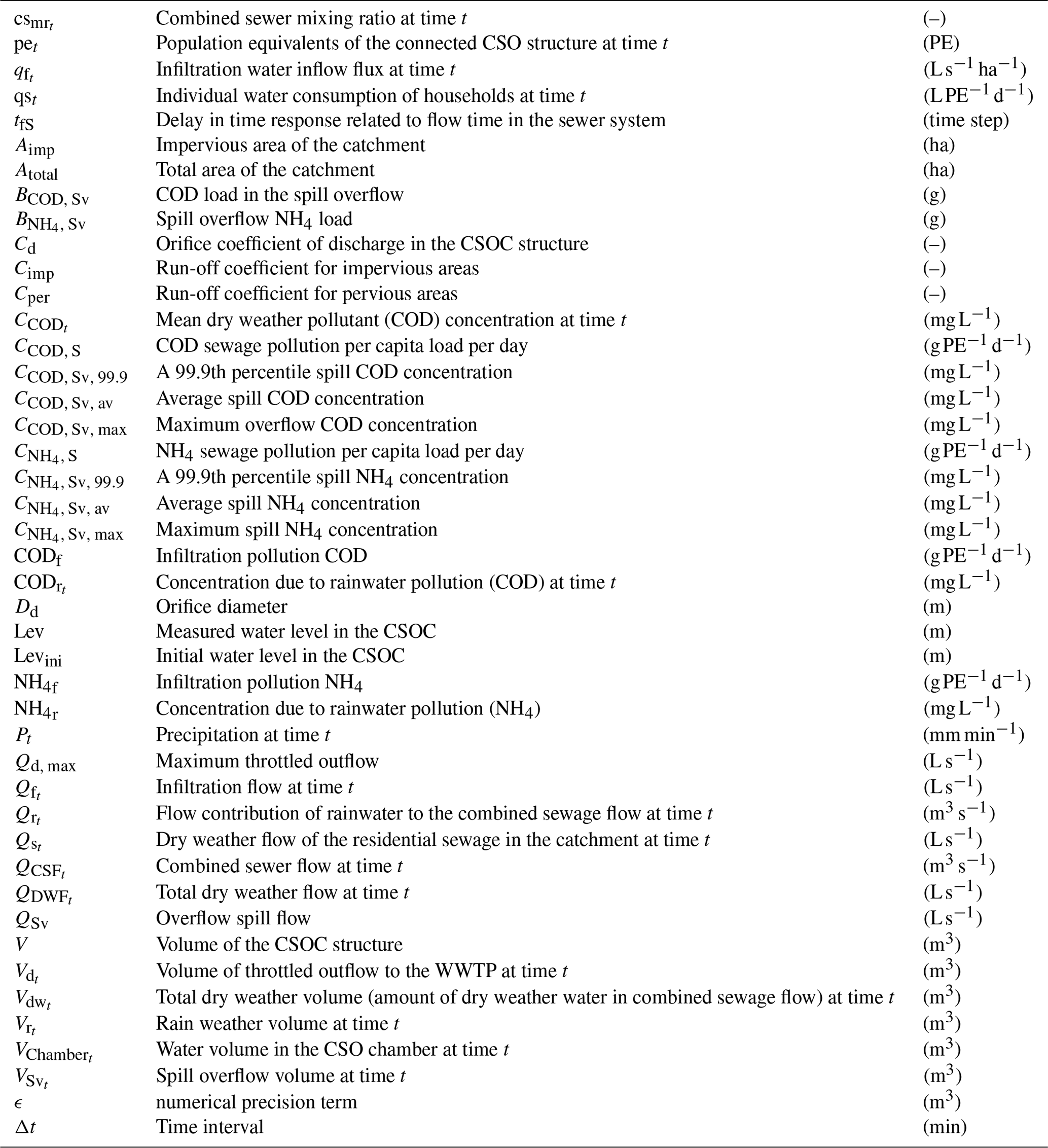
EmiStatR is used to simulate CSO flows and water quality concentrations. Details regarding the conceptual and mathematical model are provided in Torres-Matallana et al. (2018b). A list of the EmiStatR inputs and outputs is provided in Appendix A. The main components of the EmiStatR model are (1) dry weather flow (DWF), including infiltration flow (IF), (2) pollution of DWF, (3) rain weather flow (RWF), (4) pollution of RWF, (5) combined sewer flow (CSF) and pollution, and (6) combined sewer overflow (CSO) and pollution. Figure 1 illustrates the scheme of the sewer system analysed.

Figure 1 Scheme of the sewer system analysed. Adapted from Andrés-Doménech et al. (2010)

Basically, the total dry weather flow, Q_DWF (L s⁻¹), is calculated as follows:

$$\begin{array}{}\text{(1)}& Q_{{\mathrm{DWF}}_t}=Q_{{\mathrm{s}}_t}+Q_{{\mathrm{f}}_t},\end{array}$$

where $Q_{{\mathrm{DWF}}_t}$ (L s⁻¹) is the dry weather flow at time t, and $Q_{{\mathrm{s}}_t}$ (L s⁻¹) is the dry weather flow of the residential sewage in the catchment at time t, calculated as 86 400⁻¹ pe_t qs_t (where $\mathrm{86}\mathrm{400}=\mathrm{24}\times \mathrm{60}\times \mathrm{60}$ is a measurement unit conversion factor), with pe_t (PE) the population equivalents of the connected CSO structure at time t, and qs_t $\left(\mathrm{L}{\text{PE}}^{-\mathrm{1}}{\text{d}}^{-\mathrm{1}}\right)$ is the individual water consumption of households at time t. $Q_{{\mathrm{f}}_t}$ (L s⁻¹) is the infiltration flow at time t that enters the pipes from groundwater flow through cracks and joints, calculated as $A_{\mathrm{imp}}\cdot q_{{\mathrm{f}}_t}$, where A_imp (ha) is the impervious area of the catchment, and $q_{{\mathrm{f}}_t}$ $\left(\mathrm{L}{\mathrm{s}}^{-\mathrm{1}}{\text{ha}}^{-\mathrm{1}}\right)$ is the infiltration water inflow flux (specific infiltration discharge from groundwater flow) at time t. Variables qs_t and pe_t are dynamic and can be defined as time series with daily, weekly, and seasonal patterns.

The contribution of rainwater to the combined sewage flow, Q_r (m³ s⁻¹), is derived from precipitation as follows:

$$\begin{array}{}\text{(2)}& Q_{{\mathrm{r}}_t}={\displaystyle \frac{\mathrm{1}}{\mathrm{6}}}\cdot P_{t-t_{\mathrm{fS}}}\cdot [C_{\mathrm{imp}}\cdot A_{\mathrm{imp}}+C_{\mathrm{per}}\cdot (A_{\mathrm{total}}-A_{\mathrm{imp}}\left)\right],\end{array}$$

where $\frac{\mathrm{1}}{\mathrm{6}}$ is a factor for units conversion, $P_{t-t_{\mathrm{fS}}}$ is precipitation at time t−t_fS (mm min⁻¹), t_fS is a delay in time response related to flow time in the sewer system, A_imp is the impervious area of the catchment (ha), A_total is the total area of the catchment (ha), C_imp is the run-off coefficient for impervious areas (–), and C_per is the run-off coefficient for pervious areas (–). From $Q_{{\mathrm{r}}_t}$, the CSO volume calculation is based on the exceeding volume stored in the combined sewer overflow chamber (CSOC). The CSO volume depends on four CSOC stages, namely (1) filling up, (2) CSO spill volume, (3) stagnation, and (4) emptying. The sum of the total dry weather flow, $Q_{{\mathrm{DWF}}_t}$, and the rain water flow, $Q_{{\mathrm{r}}_t}$, is called combined sewer flow at time t, $Q_{{\mathrm{CSF}}_t}$.

The COD load, B_COD, Sv (g), in the spill overflow volume is calculated as a function of the spill overflow volume at time t, $V_{{\mathrm{Sv}}_t}$ (m³), a combined sewer mixing ratio at time t, ${\mathrm{cs}}_{{\mathrm{mr}}_t}$ (–), the mean dry weather pollutant concentration at time t, $C_{{\mathrm{COD}}_t}$ (mg L⁻¹), and the concentration due to rainwater pollution at time t, ${\mathrm{COD}}_{{\mathrm{r}}_t}$ (mg L⁻¹) as follows:

$$\begin{array}{}\text{(3)}& B_{\mathrm{COD},{\mathrm{Sv}}_t}={\left({\mathrm{cs}}_{{\mathrm{mr}}_t}+\mathrm{1}\right)}^{-\mathrm{1}}{V}_{{\mathrm{Sv}}_t}\left({\mathrm{cs}}_{{\mathrm{mr}}_t}\cdot C_{{\mathrm{COD}}_t}+{\mathrm{COD}}_{{\mathrm{r}}_t}\right).\end{array}$$

The variable $V_{{\mathrm{Sv}}_t}$ depends directly on the water volume in the CSO chamber at time t, $V_{{\mathrm{Chamber}}_t}$ (m³). It is computed as follows:

$$\begin{array}{}\text{(4)}& {V_{\mathrm{Sv}}}_t=\left\{\begin{array}{ll}{V}_{{\mathrm{r}}_t}+V_{{\mathrm{dw}}_t}-V_{{\mathrm{d}}_t},& \text{if}{V_{\mathrm{Chamber}}}_t=V,\\ {V_{\mathrm{Chamber}}}_t-V& \text{if}{V_{\mathrm{Chamber}}}_t>V,\\ \mathit{ϵ}& \text{if}{V_{\mathrm{Chamber}}}_t<V,\end{array}\right.\end{array}$$

where $V_{{\mathrm{r}}_t}$ is the rain weather volume at time t accumulated during a time interval Δt (min), $V_{{\mathrm{dw}}_t}$ (m³) is the total dry weather volume (amount of dry weather water in combined sewage flow) at time t, $V_{{\mathrm{d}}_t}$ is the volume of throttled outflow to the wastewater treatment plant (WWTP) at time t (m³), V (m³) is the CSOC volume, and ϵ is a numerical precision term set equal to 10⁻⁵ (m³). While V_Sv, cs_mr, and C_COD are dynamic, ${\mathrm{COD}}_{{\mathrm{r}}_t}$ can either be dynamic or assumed constant if the pollution concentration is assumed constant in time. $C_{{\mathrm{COD}}_t}$ (mg L⁻¹) is calculated as follows (Torres-Matallana et al., 2018b):

$$\begin{array}{}\text{(5)}& {C_{\mathrm{COD}}}_t={\displaystyle \frac{{\mathrm{10}}^{\mathrm{3}}\cdot {\mathrm{pe}}_t\cdot C_{\mathrm{COD},\mathrm{S}}}{{\mathrm{qs}}_t\cdot {\mathrm{pe}}_t+\mathrm{86}\mathrm{400}\cdot A_{\mathrm{imp}}\cdot q_{{\mathrm{f}}_t}}},\end{array}$$

where C_COD, S is the COD sewage pollution per capita (PE) load per day $\left(\mathrm{g}{\text{PE}}^{-\mathrm{1}}{\text{d}}^{-\mathrm{1}}\right)$. Similar equations, as above, apply to the second water pollution indicator NH₄.

2.2 Sewer system in the Haute-Sûre catchment

The study area is composed of three sub-catchments of the Haute-Sûre catchment in the northwest of Luxembourg. The combined sewer system drains three villages, namely Goesdorf (GOE), Kaundorf (KAU), and Nocher-Route (NOR). The local sewer system downstream of each village has a CSO structure to store pollutant peaks in the first flush of combined sewage flows. Figure 2 depicts the location of the CSO structures and the delineation of the sub-catchments. The main land use types in the villages are residential, smaller industries, and farms. Outside the villages, forest and agricultural arable and grassland are the dominating land uses. The receiving water bodies of the CSO structures are tributaries of the river Sûre (or Sauer in German).

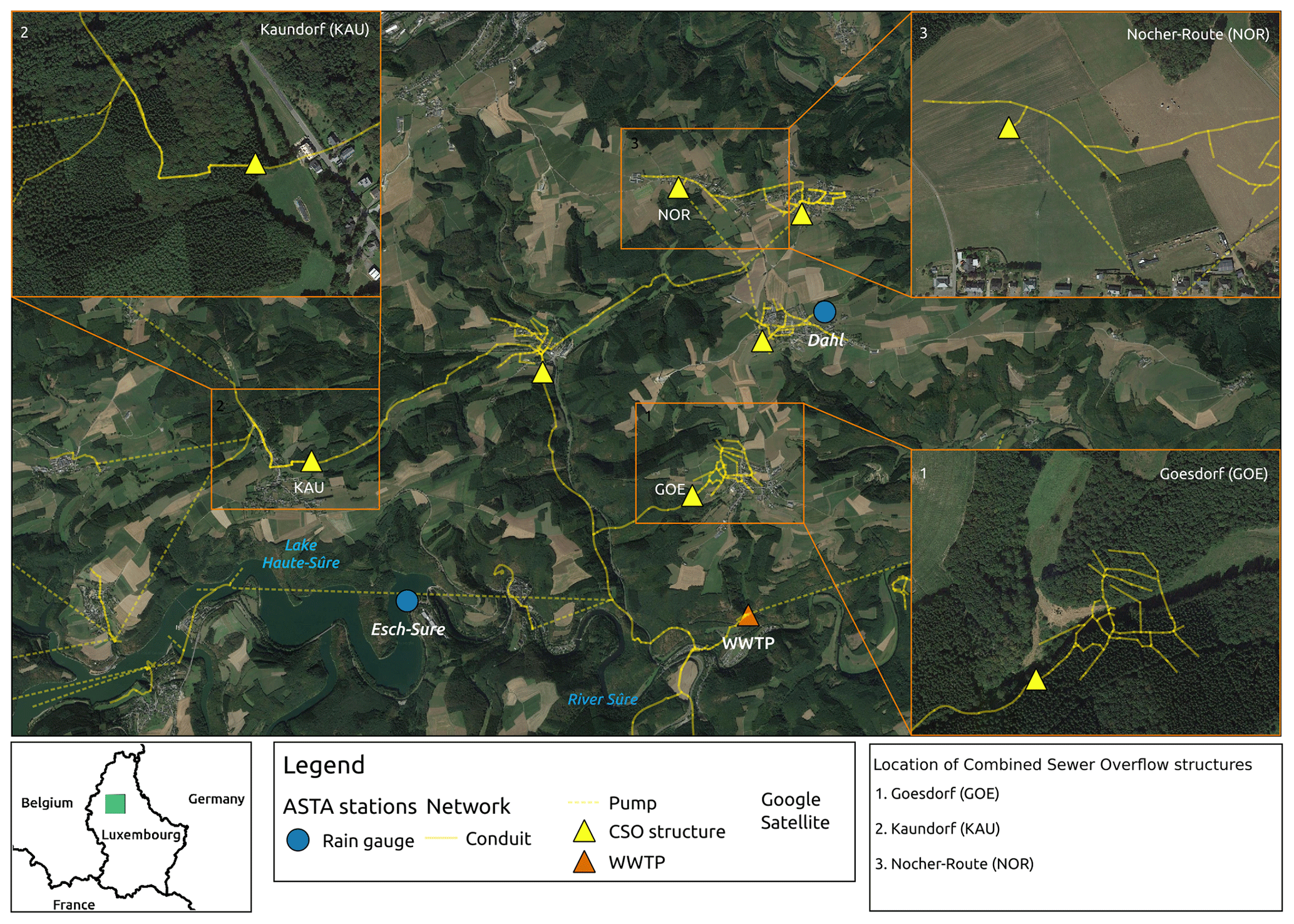
Figure 2 The three Haute-Sûre sub-catchments and locations of the combined sewer overflow (CSO) structures considered in this study. The background map is provided by © Google Maps.

2.3 Input data

The input variables of the EmiStatR model are shown in Table S1 in the Supplement. Following Torres-Matallana et al. (2018b), seven input variables were calibrated, namely water consumption (qs_t), infiltration flow ($q_{{\mathrm{f}}_t}$), flow time structure equivalent to the time of concentration to the combined sewer overflow structure (t_fS), run-off coefficient for impervious area (C_imp), run-off coefficient for pervious area (C_per), orifice coefficient of discharge (C_d), and the initial water level (Lev_ini). The main objective of the calibration process is to appropriately represent the water volume in the CSOC.

The observed precipitation (P_t) is a 1 year time series for 2010 at a 10 min time interval, measured at stations Esch-sur-Sûre and Dahl (Fig. 2). The variable water consumption (qs_t) is also dynamic and represented as a time series with a daily pattern according to factors proposed in the German ATV-DVWK-A 134 guideline (Evers et al., 2000).

The hydraulic variable measured is the water level in the CSOC, namely Lev (m). The temporal resolution of the measurements of Lev is 30 s. Regarding the wastewater quality (WWQ) characterisation, values of C_COD, S and $C_{{\mathrm{NH}}_{\mathrm{4}},\mathrm{S}}$ in the wastewater were derived from DWF measurements at Goesdorf, Kaundorf, and Nocher-Route. A total of 91 2 h composite samples were taken and measured in the laboratory to determine the concentrations of COD (mg L⁻¹) and NH₄ (mg L⁻¹). This led to the identification of seven at Goesdorf on 4 May 2011, 48 between 19 June and 21 July 2010 at Kaundorf, and 36 between 9 March and 2 August 2011 at Nocher-Route. The variables COD_f and ${{\mathrm{NH}}_{\mathrm{4}}}_{\mathrm{f}}$ were set to zero because the pollution contribution of the infiltration water is negligible in the study area. The contribution of ammonium from rainwater ${{\mathrm{NH}}_{\mathrm{4}}}_{\mathrm{r}}$ was assumed constant and set to 2.00 mg L⁻¹, while COD_r was equal to zero. Table S1 summarises the base values of the general input variables, and Table S2 presents the general characteristics of each CSO structure for each village and the base values of input variables. These base values were used when running EmiStatR in the deterministic mode (see Sect. 3.1). Some of the variables were calibrated based on observations in the CSOC to simulate water level and concentrations and loads of pollutants spilled in the CSO to the stream, river, or lake. These variables are water consumption (qs), infiltration flow (q_f), time flow (t_fS), run-off coefficient for the impervious area (C_imp), run-off coefficient for the pervious area (C_per), orifice coefficient of discharge (C_d), and initial water level (Lev_ini).

2.4 Selection of model input for uncertainty quantification

Following recommendations from Nol et al. (2010), not all model inputs were taken into account in the uncertainty propagation analysis. Only inputs that are very uncertain and to which the model output is very sensitive were included because these are the ones that have the largest contribution to output uncertainty (Heuvelink, 1998; Sect. 4.4). The level of uncertainty of the inputs was defined by expert judgement and similar case studies in the literature. A quick scan was used to determine the model sensitivity to each of the model inputs by running EmiStatR in deterministic mode with input base values given in Table S1. The level of model sensitivity was defined by analysing the mathematical model structure and components of the model, expert judgement, and simulations with EmiStatR. Inputs that rank high on both the level of uncertainty and on model sensitivity were selected and included in the uncertainty propagation analysis.

2.5 Uncertainty quantification of selected model input

Because we used a statistical approach, probability distribution functions (pdf's) are the basis for representing the uncertainties of the selected model inputs. This constitutes the most difficult step of an uncertainty propagation analysis and is done in different ways for constants and dynamic variables, as explained in the following sub-sections.

2.5.1 Uncertain constants

Following Heuvelink et al. (2007), an uncertain continuous numerical constant C can be characterised by its marginal (cumulative) pdf (mpdf) as follows:

$$\begin{array}{}\text{(6)}& F_C\left(c\right)=P(C\le c).\end{array}$$

Usually, a parametric approach can be taken, meaning that a common shape for F_C is chosen (e.g., normal, lognormal, exponential, or uniform) so that the mpdf is reduced to a number of parameters. In this study, the input variables that are in this category are water consumption (qs), infiltration inflow (q_f), total area (A_total), impervious area (A_imp), the run-off coefficients for impervious area (C_imp) and pervious area (C_per), population equivalents (pe), flow time structure (t_fS), and initial water level (Lev_ini).

2.5.2 Univariate autoregressive modelling

Dynamic uncertain inputs may be temporally autocorrelated. This may dramatically influence the outcome of an uncertainty propagation analysis and must therefore be accounted for. One way of doing this is by assuming an autoregressive order one (AR(1)) model as follows:

$$\begin{array}{}\text{(7)}& \begin{array}{rl}& y_t=\mathit{\mu }+\mathit{\varphi }\left(y_{t-\mathrm{1}}-\mathit{\mu }\right)+w_t,t=\mathrm{1},\mathrm{2},\mathrm{\dots },T,\\ & y_{\mathrm{0}}\sim \mathcal{N}(\mathit{\mu },{\mathit{\sigma }}^{\mathrm{2}}),\end{array}\end{array}$$

where y_t is the uncertain input at time t, μ is its mean, ϕ is the autoregressive parameter ($\mathrm{0}\le \mathit{\varphi }<\mathrm{1}$), and w_t is a Gaussian white noise time series with mean zero and variance ${\mathit{\sigma }}_w^{\mathrm{2}}$. The initial value y₀ is taken from a normal distribution with mean μ and variance σ². The parameters of the model can be estimated based on observations, or in the absence of observations, suitable values are taken based on expert judgement or literature reference values. Note that the effect of the initial condition usually fades out quickly and hence is not of great concern.

The implementation of the AR(1) model in R was done via the R function arima.sim of the R base package stats (R-Core-Team and contributors worldwide, 2017), both for model calibration and simulation.

2.5.3 Multivariate autoregressive modelling

In the case of multiple uncertain dynamic inputs, cross-correlation between these inputs may also need to be included. For example, C_COD, S and $C_{{\mathrm{NH}}_{\mathrm{4}},\mathrm{S}}$ and their uncertainties are likely correlated. This can be done using a multivariate AR(1) model (Luetkepohl, 2005), which is a natural extension of the univariate AR(1) model, as follows:

$$\begin{array}{}\text{(8)}& \begin{array}{rl}& \mathit{Y}(t+\mathrm{1})=\mathit{\mu }+\mathbf{A}\cdot \left[\mathit{Y}\right(t)-\mathit{\mu }]+\mathit{\epsilon }\left(t\right),\\ & t=\mathrm{1},\mathrm{2},\mathrm{\dots },T,Y_{\mathrm{0}}\sim \mathcal{N}(\mathit{\mu },\mathbf{\Lambda }),\end{array}\end{array}$$

where Y(t) is a vector of inputs at time t, A is a square matrix with parameters that define how the variables at time t+1 depend on those at time t, μ is now a vector of means, and ε(t) is a vector of zero-mean normally distributed white noise processes. We further assume that the variance–covariance matrix C of ε(t) is time invariant. The initial value Y₀ is assumed normally distributed and uncorrelated (Λ is a diagonal matrix). In order to estimate the vector μ and matrices A and C, a sample of the variables of interest is needed. Parameter estimation is done by means of the R package mAr (Barbosa, 2015).

2.5.4 Input precipitation model

In case precipitation is selected as an uncertain input to be included in the uncertainty analysis, it too must be characterised by a pdf. Since precipitation, however, is not normally distributed and has many zeros, we cannot make the Gaussian assumption, and hence we cannot use the approach described in Sect. 2.5.2 to model its dynamic behaviour and uncertainty. In addition, we usually have precipitation measurements nearby so we need to condition the simulations to these measurements. Recall from Sect. 2.3 that, in the case study, precipitation data are recorded at stations Esch-sur-Sûre and Dahl.

Torres-Matallana et al. (2017) present a model to simulate precipitation inside a target catchment given a known precipitation time series in a nearby location outside the catchment, while accounting for the uncertainty that is introduced due to spatial variation in precipitation. The method used for input precipitation uncertainty characterisation is essentially the same as the application of a Kalman filter/smoother (Kalman, 1960; Webster and Heuvelink, 2006). Calibration of the model requires precipitation time series at two locations near the catchment of interest. Once the model is calibrated, it is used to simulate precipitation inside the target catchment from a single precipitation time series nearby the catchment. Details of the calibration and conditional simulation are presented in Sect. S4.

2.6 Uncertainty analysis

We used a MC simulation (Hammersley and Handscomb, 1964; Kalos and Whitlock, 2008) to analyse how input uncertainty propagates through the EmiStatR model because it is flexible and straightforward to implement. It is also feasible in our case study because EmiStatR is a relatively simple model that does not involve a long computation time.

2.6.1 Monte Carlo simulation

The MC method runs the EmiStatR model repeatedly, each time using different model input values sampled from their pdf. The method thus consists of the following steps:

1. Repeat n times:

   1. Generate a set of realisations of the uncertain model inputs at 10 min resolution.

   2. Run the model at 10 min resolution and store output for this set of realisations. Later, in order to compute the summary statistics, a temporal aggregation of the model output to 1 h intervals is done.

2. Compute and store sample statistics from the n model outputs.

Here, n is the number of MC runs, i.e. the MC sample size. Common sample statistics that measure the uncertainty are the standard deviation and quantiles of the distribution of MC outputs, such as the difference between the 0.95 and 0.05 quantile, which can be easily calculated from the n MC outputs.

Sampling from the pdf of uncertain inputs was done using simple random sampling.

2.6.2 Monte Carlo output summary

Proper presentation of MC outputs is important for achieving the most from the experiment. Therefore, summary statistics are one important way to summarise the MC outputs. Commonly, a MC study yields n model outputs, which are stored in the MC result matrix X in Boos and Osborne (2015). From this matrix, various statistics can be computed. Basic summary statistics include the mean μ_MC, the standard deviation (σ_MC), and the variance ${\mathit{\sigma }}_{\mathrm{MC}}^{\mathrm{2}}$. From these, we can compute the coefficient of variation CV_MC (σ_MC∕μ_MC), which is a dimensionless expression of relative uncertainty. The coefficient of variation is a standardised measure of the spread of a sampling distribution, which is useful because it allows a direct comparison of the variation in samples with different units or with very different means (Marwick and Krishnamoorthy, 2019). We computed estimates and standard errors for these statistics and also for the interquartile range (IQR_MC), 0.005 (ζ_0.005) and 0.995 (ζ_0.995) quantiles, and the 99 % width of the prediction band (ζ_w, 0.99).

2.6.3 Bootstrap computation for Monte Carlo summary

Following Boos and Osborne (2015), who argue that “Good statistical practice dictates that summaries in MC studies should always be accompanied by standard errors,” we used the bootstrap method to compute the standard errors of all MC statistics. These tools are particularly relevant in a case without analytic solutions (Boos, 2003). According to Boos and Osborne (2015, p. 228) standard errors for MC output statistics are often not computed, which is an additional computational step on top of the overall analysis. Standard errors are straightforward to compute for simple statistics, such as the sample mean over the replications of the MC output, but are more difficult to compute for more complex statistics, such as medians, sample variances, and the classical Pearson measures of skewness and kurtosis. Therefore, to avoid burdensome computations, we opted to compute the standard errors by the bootstrap method. We briefly explain the bootstrap method below. For a detailed explanation, we refer to Efron (1979).

To compute the bootstrap variance of estimators, we follow the logic given by Boos and Osborne (2015). From a MC sample $Y_{\mathrm{1}},\mathrm{\dots },Y_n$, we draw a random sample of size n, with replacement $Y_{\mathrm{1}}^{*},\mathrm{\dots },Y_n^{*}$, and compute an estimator $\widehat{\mathit{\theta }}$ of the MC statistic θ from this resample. We independently repeat this process B times, resulting in a sample of estimators ${\widehat{\mathit{\theta }}}_{\mathrm{1}},\mathrm{\dots },{\widehat{\mathit{\theta }}}_B$. Then the bootstrap variance estimate, ${\widehat{V}}_B$, is the sample variance of this sample of estimators as follows:

$$\begin{array}{}\text{(9)}& {\widehat{V}}_B={\displaystyle \frac{\mathrm{1}}{B-\mathrm{1}}}\sum _{i=\mathrm{1}}^B{\left({\widehat{\mathit{\theta }}}_i-\overline{\widehat{\mathit{\theta }}}\right)}^{\mathrm{2}},\end{array}$$

where $\overline{\widehat{\mathit{\theta }}}$ is the mean of the sample of estimators. The MC standard error, se, is simply the square root of the bootstrap variance.

We implemented, in stUPscales (Torres-Matallana et al., 2019), specific routines for computing, by means of the bootstrap method, the MC estimators and their standard error for all MC statistics, where the variance of the model output is the most important. We compared our results with the results obtained using the Monte.Carlo.se R package (Boos et al., 2019).

2.6.4 Contributions of input variables to total uncertainty

A number of m+1 MC analyses are needed to compute the contributions of input variables to total uncertainty, where m is the number of model input variables selected for uncertainty quantification. The first MC analysis, MC_tot, is done to compute the total output uncertainty by stochastically varying all input variables. The uncertainty associated with the first variable x₁ is quantified by a second MC analysis MC₁ in which only x₁ is equal to its deterministic value, while the other input variables vary stochastically. Similarly, the other MC simulations MC₂, MC₃,  … , and MC_m are used to quantify the uncertainty for the variables x₂, x₃, … , and x_m.

To quantify the contributions of individual input variables to the total uncertainty of the model inputs, the stochastic sensitivity S_i for each uncertain input x_i is computed. It is defined as follows:

$$\begin{array}{}\text{(10)}& S_i=\mathrm{1}-{\displaystyle \frac{\mathrm{Var}\left({\mathrm{MC}}_i\right)}{\mathrm{Var}\left({\mathrm{MC}}_{\mathrm{tot}}\right)}}.\end{array}$$

The index represents the main effect contribution of each input factor to the total variance of the output. The larger the index, the more important the input uncertainty. We computed stochastic sensitivity indices per time step and aggregated contributions for the whole year. For plotting purpose, we aggregated the outputs from a 10 min time step to hourly time steps. The aggregation was done for each individual MC run before the contributions were computed.

2.7 Water quality impact

The results of the MC uncertainty propagation were also compared with the water quality standards. Standards are introduced to evaluate the impact of emissions of COD and NH₄ in CSOs in the receiving water. However, as Toffol (2006) recognises, although there are European emission standards for wastewater treatment plant effluent, standards for combined sewer overflow are not so clear. According to Steinel and Margane (2011), the European Water Framework Directive (WFD) is mainly concerned with the natural state of waters. Therefore, emission standards for effluent discharge are not set. The European Union Council Directive 91/271/EEC (1991) sets standards for COD and total nitrogen; hence, similar values have been adopted in many European member states. For more details about guidelines and design procedures in Europe, see Blumensaat et al. (2012). We assessed the emissions according to the German guideline ATV-DVWK-A 128 (1992), which is the standard for the dimensioning and design of storm water structures in combined sewers and commonly used in Luxembourg. The Austrian ÖWAV-RB 19 (2007) is also taken into account because it provides key reference guidelines for the design of urban water infrastructure in central Europe. Three main indicators are taken into account, namely hydraulic impact, COD concentration, and acute ammonium toxicity.

2.7.1 Hydraulic impact

According to the Austrian guidelines, and as summarised by Kleidorfer and Rauch (2011), the evaluation of the hydraulic impact is given by the following:

$$\begin{array}{}\text{(11)}& Q_{\mathrm{1}}\le f_{\mathrm{h}}\cdot Q_{\mathrm{r}\mathrm{1}},\end{array}$$

where $\mathrm{0.1}\le f_{\mathrm{h}}\le \mathrm{0.5}$, Q₁ (L s⁻¹) is the maximum sewer overflow discharge with return period of 1 year, and Q_r1 (L s⁻¹) is the maximum water discharge in the river with return period of once per year. The factor f_h is taken as 0.1 in more sensitive streams, whereas it is 0.5 for streams with more stable bed and higher re-colonisation potential Toffol (2006). Time series of daily values recorded in 2006 to 2013 of the river Sûre at Heiderscheidergrund were used to compute the daily flow expected, with a return period of once per year (1.01 years), Q_r1.

We used the German guideline ATV-DVWK-A 128 (1992), which computes the throttle discharge at CSOs, Q_t, CSO (L s⁻¹) as follows:

$$\begin{array}{}\text{(12)}& Q_{t,\mathrm{CSO}}=f_t\cdot A_{\mathrm{imp}},\end{array}$$

where $\mathrm{7.5}\le f_t\le \mathrm{15}$ and A_imp (ha) are the impervious areas connected to the combined sewer system. For the overflow flow MC output mean, the 0.95 and 0.995 quantile, we computed the exceedance percentage over the thresholds, which is calculated as the proportion of time steps exceeding the number of total time steps in the year (8759 time steps at 1 h).

2.7.2 COD concentration

Steinel and Margane (2011, Table 14) present the effluent standards for discharging into freshwater adopted in selected European countries. A COD concentration of 125 mg L⁻¹ is reported for European Union countries. Austria has stricter rules, with a standard of 90 mg L⁻¹ for populations between 50 and 500 inhabitants and 75 mg L⁻¹ for populations greater than 500 inhabitants. The Goesdorf population was 1025 inhabitants by 2001 and was 1297 inhabitants by 2011 (Statec, 2020). For NH₄ a similar approach was used.

2.7.3 Acute ammonium toxicity

Following Kleidorfer and Rauch (2011), who argue that “the ammonia (NH₃) concentration depends on the ammonium (NH₄) concentration and on the dissociation equilibrium between NH₃ and NH₄ (which is influenced by temperature and pH-value)”. According to Kleidorfer and Rauch (2011), the Austrian guideline ÖWAV-RB 19 (2007) establishes a maximum value of 2.5 mg L⁻¹ for the ammonium (NH₄) concentration calculated for a 1 h duration for salmonid streams. For cyprinid streams, a maximum value of 5.0 mg L⁻¹ is recommended.

3 Results

3.1 Selection of model inputs for uncertainty quantification

In this section, we assess the degree of uncertainty and sensitivity for all input variables, following the procedure described in Sect. 2.4. We summarise the results in Tables 1 and 2. To better support our decisions, we also include a graphical assessment of the degree of uncertainty and sensitivity of each input, as in Tscheikner-Gratl et al. (2017, see Fig. S1).

3.1.1 Wastewater

Water consumption, qs, is a fairly uncertain input variable, and the model output is sensitive to this variable. Volume and flow of CSO are sensitive to changes in qs. Regarding water quality output, the total load of NH₄ is very sensitive to changes in qs. Pollution of sewage as COD load per capita per day, C_COD, S, is the first selected input variable for propagation of uncertainty, due to the fact that it is both a very uncertain input variable and the model output (average and 99.9 percentile overflow COD concentration) is very sensitive to it. Pollution of sewage as NH₄ load per capita per day, $C_{{\mathrm{NH}}_{\mathrm{4}},\mathrm{S}}$, is also included in the uncertainty propagation analysis. It is a very uncertain input variable, and the model output (overflow load and concentrations of NH₄) is very sensitive to it. The variables C_COD, S and $C_{{\mathrm{NH}}_{\mathrm{4}},\mathrm{S}}$ are very uncertain because these are correlated to the temporal and spatial pattern of water consumption, which has a daily, weekly, and seasonal temporal variability.

3.1.2 Infiltration water

Inflow of infiltration water, q_f, is a very uncertain input variable because this inflow depends on the number of anomalies in the pipes (cracks or wrong connections) that allows infiltrations flowing into and out of the system. The distribution of these anomalies has a strong random component, and hence, q_f is very uncertain, and the model output is sensitive to it. Although this is a very uncertain input, the quick-scan analysis showed that model output sensitivity is not very high, as indicated in Table 1. For this reason, we did not include this variable in the uncertainty propagation analysis.

Pollution of infiltration water as COD load per capita per day, COD_f, and pollution of infiltration water as NH₄ load per capita per day, ${{\mathrm{NH}}_{\mathrm{4}}}_{\mathrm{f}}$, are not uncertain because in the Haute-Sûre study area the values of these variables are negligible.

Table 1 Results of deterministic sensitivity analysis. Average percentage of change in model output caused by ±10 % change in model inputs (qs, C_COD, S, $C_{{\mathrm{NH}}_{\mathrm{4}},\mathrm{S}}$, COD_r, pe, and P as time series; VAR(1) model for C_COD, S and $C_{{\mathrm{NH}}_{\mathrm{4}},\mathrm{S}}$; and AR(1) model for COD_r and AR(1) conditioned for P; see Appendix A for nomenclature definitions). Output change greater than 15 % is considered very high. Variable C_d (not shown in the table) leads to a percentage of change of less than 0.3 %, while variables t_fS and Lev_ini (not shown in the table) lead to no change in the output. Values greater than 15 are shown in bold.

3.1.3 Rainwater

Precipitation, P, is the main driving force of the model, and given the spatial variability of the rain fields, this input is considered very uncertain. The model output, additionally, is very sensitive to it. As a consequence, this input variable is treated as the third input variable in the uncertainty propagation analysis. Pollution of run-off as COD concentration, COD_r, is the fourth input variable considered in the uncertainty propagation, given that it is a very uncertain and very sensitive input variable, particularly to the load and concentration of COD in the overflow.

Pollution in rainwater as NH₄ concentration, ${{\mathrm{NH}}_{\mathrm{4}}}_{\mathrm{r}}$, is considered fairly uncertain. The model output (overflow load and concentration of NH₄) is very sensitive to it. Although model output is very sensitive to this model input variable, model input uncertainty is not very high, as indicated in Table 1. For this reason, it was not included in the uncertainty propagation analysis.

3.1.4 Sub-catchment

The model is very sensitive to the total area A_total and to the run-off coefficient for the pervious area (C_per) and sensitive to the impervious area A_imp and to the run-off coefficient for impervious area (C_imp). However, we did not include A_total in the uncertainty analysis because it can be fairly accurately derived from spatial databases, and hence, their uncertainty is not large. Although model output is very sensitive to the input variable C_per, the uncertainty about this variable is not very high, as indicated in Table 1. The reason behind this is that C_per can be derived fairly accurately from geographic information system (GIS) products, such as land use and soil type maps. Therefore, we did not include this variable in the uncertainty propagation analysis. The population equivalents, pe, is a sensitive variable but not very uncertain. Hence, this variable was not included in the uncertainty analysis. The theoretical largest flow time in the catchment t_fS is not uncertain and not sensitive.

3.1.5 CSO structure

Although model output is very sensitive to maximum throttled outflow Q_d, max and volume V, these are not included in the uncertainty analysis because their values are accurately known. The same is true for the variables curve level–volume lev2vol, orifice diameter D_d, and discharge coefficient C_d. These variables are accurately known and, therefore, not considered as being uncertain variables. The initial water level in the chamber Lev_ini is very uncertain, but the model output is not sensitive to this variable. Therefore, Lev_ini was not included in the uncertainty analysis.

3.2 Uncertainty quantification of selected model input

After ranking all inputs on levels of uncertainty and model sensitivity, we selected four input variables to be included in the uncertainty analysis. These are C_COD, S, $C_{{\mathrm{NH}}_{\mathrm{4}},\mathrm{S}}$, COD_r, and P (Table 2).

3.2.1 Sewage per capita COD and Ammonium

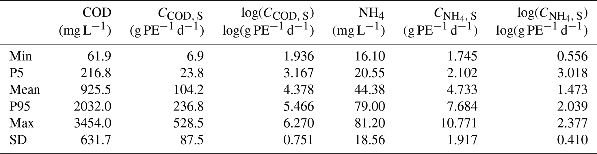
The fit of pdf's for the two uncertain inputs, C_COD, S and $C_{{\mathrm{NH}}_{\mathrm{4}},\mathrm{S}}$, was based on measurements under dry weather flow conditions. Measurement campaigns were done in Goesdorf from 28 April to 24 June 2011, in Kaundorf from 22 June to 18 August in 2010 and from 20 July to 5 August in 2011, and in Nocher-Route from 18 November 2010 to 27 April 2011. Samples of COD and NH₄ in mg L⁻¹ (91 in total for each variable) were analysed. An average wastewater amount was calculated for Goesdorf (153 L PE⁻¹ d⁻¹), Kaundorf (112 L PE⁻¹ d⁻¹), and Nocher-Route (94.3 L PE⁻¹ d⁻¹). Table 3 presents summary statistics of the dry weather flow measurements of COD and NH₄ and the corresponding value of C_COD, S and $C_{{\mathrm{NH}}_{\mathrm{4}},\mathrm{S}}$. COD is converted to C_COD, S by means of a simple conversion from mg L⁻¹ to g PE⁻¹ d⁻¹, by multiplying COD by the measured per capita flow (112 L PE⁻¹ d⁻¹) and dividing by 1000. NH₄ was converted to $C_{{\mathrm{NH}}_{\mathrm{4}},\mathrm{S}}$ in a similar way.

Table 2 Input variables of the EmiStatR model and selection of inputs for uncertainty analysis based on input uncertainty level and model sensitivity level (Note: ++ is very uncertain/sensitive; – – is not uncertain/sensitive).

Table 3 Summary statistics of dry weather flow measurements for C_COD, S and $C_{{\mathrm{NH}}_{\mathrm{4}},\mathrm{S}}$ characterisation.

Closer inspection showed that C_COD, S and $C_{{\mathrm{NH}}_{\mathrm{4}},\mathrm{S}}$ observations are best characterised by a lognormal distribution (Sect. S5). Since C_COD, S and $C_{{\mathrm{NH}}_{\mathrm{4}},\mathrm{S}}$ are dynamic and cross-correlated, we calibrated a bivariate AR(1) model with state vector $\mathit{Y}=\left[\text{log}\right(C_{\mathrm{COD},\mathrm{S}})$ $\text{log}\left(C_{{\mathrm{NH}}_{\mathrm{4}},\mathrm{S}}\right){]}^T$. The estimated parameters of the model, using the methodology described in Sect. 2.5.3, are as follows:

$$\begin{array}{}\text{(13)}& \begin{array}{rl}& \mathit{\mu }=\left[\begin{array}{l}\mathrm{4.40947}\\ \mathrm{3.70411}\end{array}\right]\mathbf{A}=\left[\begin{array}{rr}\mathrm{0.99165}& -\mathrm{0.00319}\\ -\mathrm{0.00009}& \mathrm{0.99455}\end{array}\right]\\ & \mathbf{C}=\left[\begin{array}{ll}\mathrm{0.00913}& \mathrm{0.00224}\\ \mathrm{0.00224}& \mathrm{0.00185}\end{array}\right].\end{array}\end{array}$$

The defined multivariate autoregressive model also captures the dynamic behaviour, temporal correlation, and cross-correlation of the input variables, deriving the probability distributions of C_COD, S and $C_{{\mathrm{NH}}_{\mathrm{4}},\mathrm{S}}$ from measurements in the Haute-Sûre catchment, which agreed well with values reported in the literature (Katukiza et al., 2014; Heip et al., 1997).

3.2.2 Run-off COD concentration

Regarding COD_r, due to the fact that no field measurements were available, expert judgement and reference values from the literature were the basis for characterising the pdf of this input variable. The variable was assumed to be lognormally distributed with a mean value of 71 mg L⁻¹. Although, House et al. (1993) and Welker (2008) reported a higher value, namely 107 mg L⁻¹ for COD_r, we selected a lower value due to the specific characteristics of the CSO system in the Haute-Sûre catchment. The value of 150 mg L⁻¹ as standard deviation of COD_r leads to a coefficient of variation (SD ⋅ mean⁻¹) equal to 2.11, which is greater than the coefficient of variation for C_COD, S (0.84). We allow the standard deviation of COD_r to be greater than the standard deviation of C_COD, S because COD measurements in rain water are very uncertain.

3.2.3 Input precipitation model

Precipitation and its associated uncertainty was modelled as an autoregressive model conditioned to the observed precipitation at a nearby measurement station. We assumed a multivariate lognormal distribution and included a temporal correlation of the simulated time series. Calibration of the precipitation model is done with the mAr package, as explained in Sect 2.5.4, and using a 10 min precipitation time series of stations Esch-sur-Sûre and Dahl for 2010. Upon calibration of the multivariate autoregressive model, we proceeded with the conditional simulation of Y_c (Sect. S4.2, Eq. 5). For this, we computed the parameters of the model, as shown in Eq. (14). The model parameters are given by (Torres-Matallana et al., 2017) the following:

$$\begin{array}{}\text{(14)}& \begin{array}{rl}& \begin{array}{l}{\mathit{\mu }}_{\mathrm{1}}=\mathrm{2.85501}\\ {\mathit{\mu }}_{\mathit{\delta }}=\mathrm{0.10194}\end{array}\mathbf{B}=\left[\begin{array}{l}\mathrm{0.95650}\mathrm{0.03980}\\ \mathrm{0.02429}\mathrm{0.88304}\end{array}\right]\\ & \begin{array}{l}{\mathit{\sigma }}_{\mathrm{1}}^{\mathrm{2}}=\mathrm{0.07241}\\ {\mathit{\sigma }}_{\mathit{\delta }}^{\mathrm{2}}=\mathrm{0.07951}\\ {\mathit{\rho }}_{\mathrm{1}\mathit{\delta }}=-\mathrm{0.03876}.\end{array}\end{array}\end{array}$$

Next, we generated conditional simulations of the 10 min precipitation for 2010 for each subcatchment using the approach described in Sect. 2.5.4. Note that this involves simulating log-transformed precipitation, which can easily be transformed to precipitation data using the antilog. The simulation procedure was repeated as many times as simulated precipitation time series were required for the MC uncertainty propagation analysis.

The simulated precipitation time series captured the main statistics of the observed time series well. The reader can find evidence for this in the Supplement (Table S4 and Fig. S2). Despite the satisfactory performance of the proposed method, some cases showed an overestimation of the simulated precipitation, mainly due to high values of the ratio of the multiplicative factor δ(t). This behaviour was also recognised by McMillan et al. (2011), who stated that the multiplicative factor used in their study “does not capture the distribution tails, especially during heavy precipitation where input errors would have important consequences for run-off prediction”.

3.3 Uncertainty analysis

Model output sensitivity and the degree of uncertainties evaluation of each model input helped to define the four input variables included in the uncertainty analysis, namely C_COD, S, $C_{{\mathrm{NH}}_{\mathrm{4}},\mathrm{S}}$, COD_r, and P. In this section, we present the results of the uncertainty propagation for these four selected input variables to the model output, both for water quantity (volume in the combined sewer overflow chamber, CSOC, and overflow volume and flow) and for water quality (loads and concentrations of chemical oxygen demand, COD, and ammonium, NH₄).

3.3.1 Monte Carlo output and uncertainty quantification

The seven output variables from EmiStatR were analysed by MC input uncertainty propagation. A detailed description of the Monte Carlo simulation size and timing is presented in the Supplement (Sect. S6).

Figure 3 illustrates the uncertainty propagation outcomes for the first Monte Carlo simulation, in which all input variables vary stochastically. The MC simulations were performed for the entire year of 2010 at 10 min time steps, which were aggregated to hourly time steps in the figure. The aggregation function was used for precipitation, CSO chamber volume, CSO spill volume, and loads was the sum, whereas for CSO spill flow and concentrations the aggregation function was the mean. The top of Fig. 3 shows input precipitation as main driving input. For illustration purposes, two events with a 2 d duration each are shown. The first event occurred in spring (May 2010) and the second in autumn (September 2010), and this shows that the uncertainty is high when there is a high precipitation event. The more intense the precipitation input, as seen in Fig. 3 in the top left (May event), the greater the uncertainty bandwidth for overflow flow and for COD and NH₄ loads (Fig. 3e–h) and concentrations (Fig. 3i–l). The MC-estimated statistics and the standard errors (se) are presented in Table 4. The table shows the uncertainty quantification of outputs obtained from the MC uncertainty propagation for the first MC simulation (all selected input variables are uncertain).

Table 4 Monte Carlo estimated statistics and standard errors (se) determined by bootstrapping for the MC simulations, where all selected input variables are uncertain R (model was run at 10 min time steps, and MC results were aggregated to 1 h averages over a 1 year period). See Appendix A for output variable nomenclature and units. Note: Interq. – interquartile; quant. – quantile; pbw – prediction band width; SD – standard deviation; var – variance; cv – coefficient of variation.

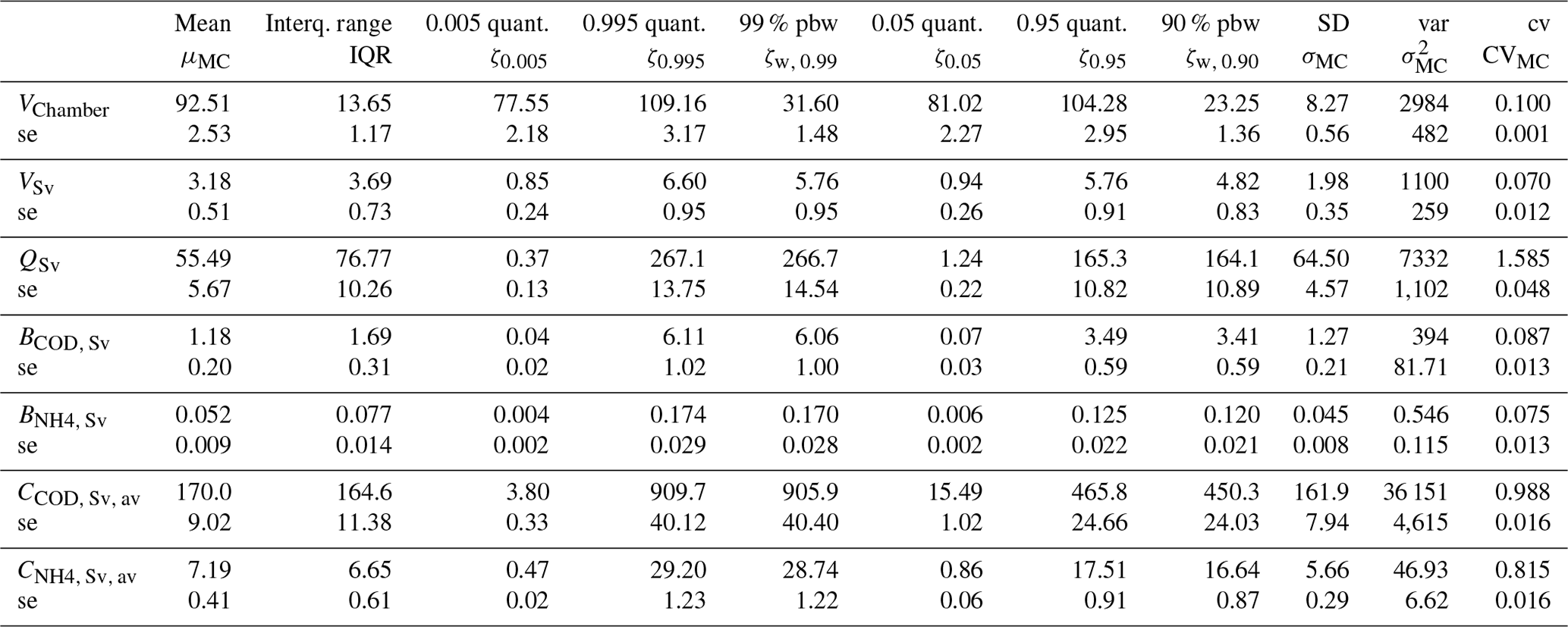
Table 4 shows the standard deviation (SD) and the coefficient of variation (cv) for the seven output variables considered in the uncertainty propagation. For the volume in the CSO chamber, V_Chamber, the annual mean standard deviation, σ_MC, (8.27 m³) is lower than the mean, μ_MC, (92.51 m³). This goes along with an annual mean coefficient of variation (CV_MC) of 0.100. A (CV_MC) greater than one means large uncertainty. The overflow spill volume, V_Sv, had a coefficient of variation of 0.070, while it was 1.585 for the overflow flow, Q_Sv. This shows that the relative uncertainty of the overflow flow is very large. Regarding the overflow COD load, the annual mean (1.18 kg) is similar as the annual mean standard deviation (1.27 kg). Similar behaviour was observed for the overflow COD concentration, which had an annual mean value of 170 mg L⁻¹ and a standard deviation of 162 mg L⁻¹. For overflow NH₄ load and overflow NH₄ concentration, the annual mean also had the same order of magnitude as the annual mean standard deviation. Overflow COD and NH₄ loads had a coefficient of variation of 0.087 and 0.075, respectively, whereas the coefficient of variation for concentrations were 0.988 and 0.815, respectively. This suggests that overflow concentrations are more uncertain.

Low standard errors (se) for the coefficient of variation were obtained for all seven outputs. These were never greater than 0.05, which indicates that the selected MC replication size (1500 for mc1) is a suitable value. This holds for all output statistics because, in all cases, the standard error is small in comparison to the estimated value.

3.3.2 Contributions of input variables to total uncertainty

The contributions of input variables to the total uncertainty of the model inputs were also computed using the procedure described in Sect. 2.6.4. A total of four MC simulations with a total of 6000 runs were performed to estimate S_i (Eq. 10). Afterwards, four contributions were evaluated per time step and aggregated for the whole year. Following Eq. (10), the per time step contribution of input variables to output variables in terms of percentage of variance, stochastic sensitivity S_i of the input variables C_COD, S, $C_{{\mathrm{NH}}_{\mathrm{4}},\mathrm{S}}$, COD_r, and P were calculated. An example of the contributions analysis per time step is presented in Fig. 4. Here we remark that a high uncertainty over time is shown mainly for the spring event.

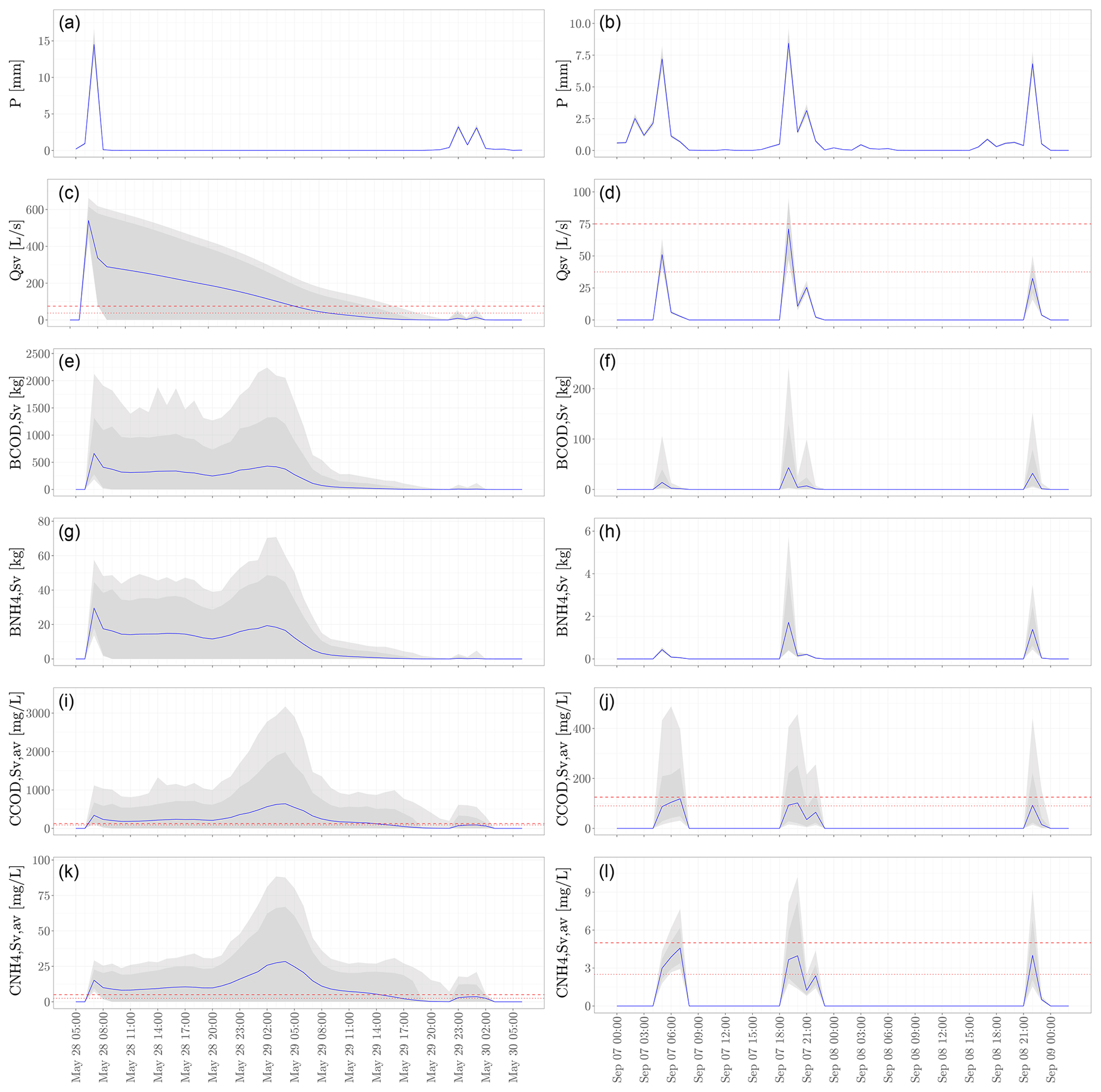
Figure 3 Uncertainty propagation outcomes for the first Monte Carlo simulation, where all input variables vary stochastically. The 99 % prediction interval is shown as a light grey shading, the 90 % prediction interval as a dark grey shading, and the mean value as a blue line. The MC simulations were performed for the entire year of 2010 at a 10 min time step, aggregated to hourly time steps in the figure. (a, b) Input precipitation. (c, d) In the overflow spill flow, the upper dashed red line indicates the 75 L s⁻¹ threshold and the lower dotted red line the 37.5 L s⁻¹ threshold. (e, f) Load of overflow COD. (g, h) Load of overflow NH₄. (i, j) In the average spill COD concentration, the upper dashed red line indicates the 125 mg L⁻¹ threshold, and the lower dotted red line indicates the 90 mg L⁻¹ threshold. (k, l) In the average spill NH₄ concentration, the upper dashed red line indicates the 5.0 mg L⁻¹ threshold and lower dotted red line the 2.5 mg L⁻¹ threshold.

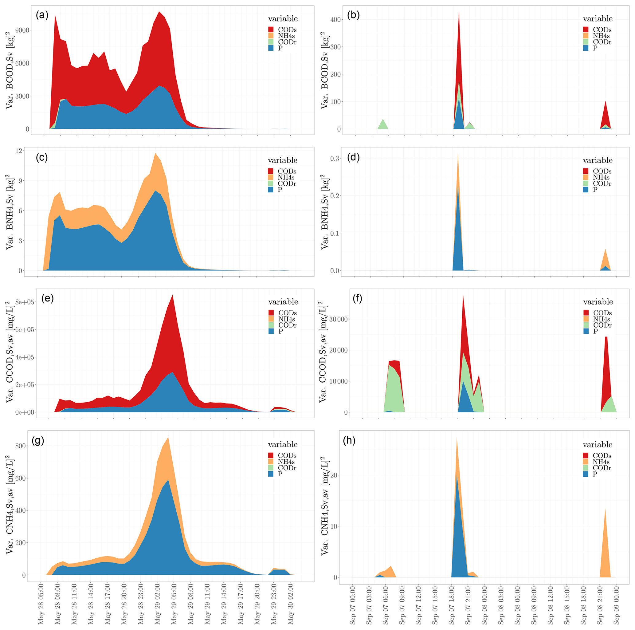
Figure 4 (a, b) Temporal contributions of input variables to the load of overflow COD, (c, d) load of overflow NH₄, (e, f) concentration of overflow COD, and (g, h) concentration of overflow NH₄ in terms of variance. The MC simulations were performed for the entire year of 2010 at a 10 min time step, which were aggregated to hourly time steps. For illustration, two periods are shown from 28 to 30 May 2010 (left) and from 7 to 9 September 2010 (right). In the legend, CODs refers to C_COD,S, and NH4s refers to $C_{{\mathrm{NH}}_{\mathrm{4}},\mathrm{S}}$.

The aggregated-over-time contributions of input variables to output variables in terms of percentage of variance and stochastic sensitivity S_i of the input variables were also calculated (Table 5). Note that P is the only source of uncertainty for V_Chamber and V_Sv, while uncertainty in NH₄ inputs only propagates to NH₄ outputs, which is similar for COD (Fig. 4).

Table 5 Aggregated-over-time contribution of input variables to output variables in terms of percentage of total variance.

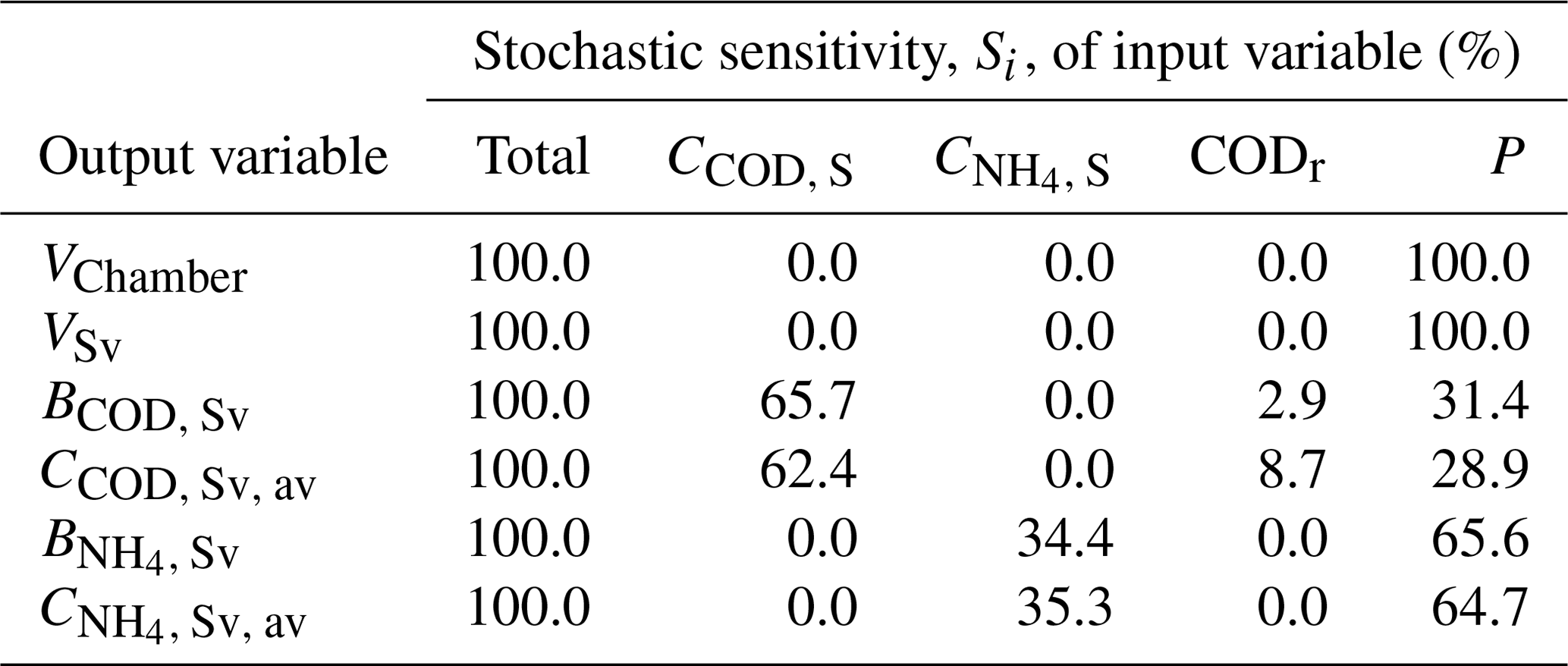
We found, as expected, that precipitation, P, is the only source of uncertainty from all uncertain input considered for water quantity output variables V_Chamber and V_Sv. Regarding average values for the whole year, for the water quality output variables B_COD, Sv and $C_{\mathrm{COD},\mathrm{Sv},\mathrm{av}}$, C_COD, S has the largest contribution to the output variance, which is about 66 % for B_COD, Sv and about 62 % for $C_{\mathrm{COD},\mathrm{Sv},\mathrm{av}}$. The second variable that contributes to the uncertainty of these COD output variables is P, with about 3 % for B_COD, Sv and 9 % for $C_{\mathrm{COD},\mathrm{Sv},\mathrm{av}}$. Similarly, the input variable $C_{{\mathrm{NH}}_{\mathrm{4}},\mathrm{S}}$ plays an important role in the contribution of total uncertainty for $B_{{\mathrm{NH}}_{\mathrm{4}},\mathrm{Sv}}$ (on average about 34 % of the variance for the whole year) and $C_{{\mathrm{NH}}_{\mathrm{4}},\mathrm{Sv},\mathrm{av}}$ (about 35 %). Equally contributing to the uncertainty of these NH₄ output variables is P with about 66 % for $B_{{\mathrm{NH}}_{\mathrm{4}},\mathrm{Sv}}$ and 65 % for $C_{{\mathrm{NH}}_{\mathrm{4}},\mathrm{Sv},\mathrm{av}}$. From these results, we can infer that precipitation is a main source of uncertainty for all six outputs considered.

3.4 Uncertainty and water quality impact

Quantification and assessment of the water quality impact is an important step after the uncertainty propagation. As described in Sect. 2.7, the assessment of water quality standards was done by taking into account the reference thresholds recommended in the European Union guidelines for COD and the German and Austrian guidelines for hydraulic impact and acute ammonium toxicity.

3.4.1 Hydraulic impact

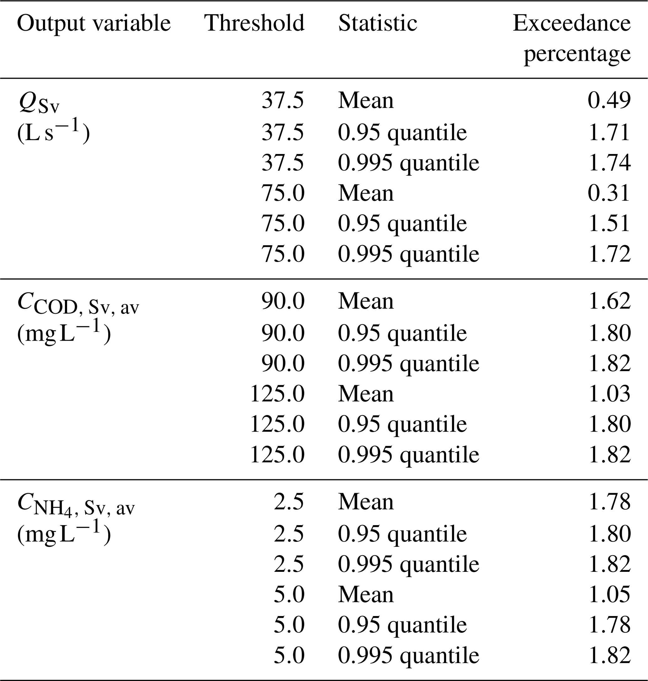
From the time series of daily values for 2006 to 2013 of the river Sûre, a daily flow expected with a return period of once per year (1.01 years), Q_r1 of 16 m³ s⁻¹ was computed at Heiderscheidergrund, which corresponds with the entire catchment area of the Haute-Sûre storm water system (182.1 ha). Therefore, we estimated the river daily flow in the Goesdorf CSO structure as a proportion to 30 ha, which is equal to 2.6 m³ s⁻¹. Following Eq. (11), the maximum sewer overflow discharge with return period of 1 year, Q₁ can have a value between 0.26 and 1.32 m³ s⁻¹. Accordingly, with the German guideline ATV-DVWK-A 128 (1992; Eq. 12), two additional thresholds are defined for the maximum sewer overflow discharge with return period of 1 year for the Goesdorf catchment (A_imp=5.0 ha). Q₁ is expected to vary between 37.5 and 75.0 L s⁻¹. We contrasted these values with those obtained from the uncertainty analysis. From Table 4, we obtained a 1 h mean value for the overflow spill flow, Q_Sv, of 55.5 L s⁻¹, 90 % prediction band width of 164.1 L s⁻¹, and standard deviation of 64.5 L s⁻¹. Figure 3a and b present the overflow spill flow for the two periods chosen for illustration. The upper dashed red line indicates the 75 L s⁻¹ threshold, and the lower dotted red line indicates the 37.5 L s⁻¹ threshold. Table 6 (top) shows the exceedance percentage of overflow spill flow over the 37.5 and 75.0 L s⁻¹ thresholds for the mean, 0.95 quantile, and 0.995 quantile. We found a 0.49 % exceedance of the mean value over the 37.5 L s⁻¹ threshold and about 1.7 % for the quantiles. As expected, slightly lower percentages were found for the 75.0 L s⁻¹ threshold.

3.4.2 COD concentration

A reference COD concentration emission in CSOs was presented in Sect. 2.7.2. For the European Union, a value of 125 mg L⁻¹ is used. We obtained a 1 h average spill COD concentration with a mean of 170 mg L⁻¹, standard deviation of 162 mg L⁻¹, and a 90 % prediction band width of 450 mg L⁻¹. Figure 3i and j present the average spill COD concentration. The upper dashed red line indicates the 125 mg L⁻¹ threshold and the lower dotted red line the 90 mg L⁻¹ threshold. The mean COD concentration in the overflow volume was higher than the thresholds. However, note that when entering the river system it will quickly be diluted, suggesting that the negative impact on the environment will be dampened by the receiving water body.

Table 6 (centre row) shows the exceedance percentage of overflow COD concentration over the 90 and 125 mg L⁻¹ thresholds for the mean, 0.95 quantile, and 0.995 quantile. We found a 1.62 % exceedance of the mean value over the 90 mg L⁻¹ threshold and about 1.8 % for the quantiles. Slightly lower percentages were found for the 125 mg L⁻¹ threshold for the mean value (1.03 %). For the quantiles equal values were found as for the 90 mg L⁻¹ threshold.

3.4.3 Acute ammonium toxicity

We compared the acute ammonium toxicity reference values presented in Sect. 2.7.3 (2.5 mg L⁻¹ for the ammonium concentration calculated for a 1 h duration for salmonid streams, and for cyprinid streams, a maximum value of 5.0 mg L⁻¹) was calculated with the values we found for ammonium. An average spill NH₄ concentration with a mean of 7.19 mg L⁻¹, standard deviation of 5.66 mg L⁻¹, and 90 % prediction band width of 16.64 mg L⁻¹ was obtained. Figure 3k and l show the average spill NH₄ concentration for the two periods chosen for illustration. The ammonium (NH₄) concentrations in the overflow flow are higher than the reference values, which are given for concentrations in the river.

Table 6 (bottom row) shows the exceedance percentage of overflow NH₄ concentration over the 2.5 and 5.0 mg L⁻¹ thresholds for the mean, 0.95 quantile, and 0.995 quantile. We found a 1.8 % exceedance of the mean and quantile values over the 2.5 and 5.0 mg L⁻¹ thresholds. A slightly lower percentage (1.1 %) was found for the 5.0 mg L⁻¹ threshold with regards to mean value.

Table 6 Frequency (percentage) over time that environmental thresholds are exceeded for different statistics of the overflow spill flow, COD, and NH₄ concentration.

4 Discussion

This study aimed to select and characterise the main sources of input uncertainty in urban water systems, while accounting for temporal auto- and cross-correlation of uncertain model inputs, by propagating input uncertainty through the EmiStatR model and quantifying and assessing the contributions of each uncertainty source to model output uncertainty dynamically (over time). In the following discussion, we start with the uncertainty and water quality impact of the model outputs to the environment, in relation to the uncertainty analysis. Next, we discuss the accuracy of Monte Carlo analysis, followed by a discussion of other sources of uncertainty. Finally, we highlight some limitations and possible solutions to the approach used in this work.

4.1 Uncertainty and water quality impact

Next, we discuss how the uncertainty propagation analysis done gives additional insight regarding hydraulics, COD concentration, and the acute ammonium toxicity impact on water quality over the river Sûre due to the CSO discharges under study. After doing the uncertainty propagation analysis, we not only have the predictions of model outputs, but we also know how uncertain these are. An added value arises when we take into account the uncertainty information. For the case of the overflow spill flow, the expected model output (mean of 55.5 L s⁻¹) is below the environmental threshold of 75 L s⁻¹, but the 0.95 quantile (164.1 L s⁻¹) is very much above the threshold. This indicates that there is a considerable chance of it being above the threshold.

Regarding water quality outputs, although the mean model output for COD and NH₄ concentrations is fairly above that of the thresholds, the 0.95 quantile is 2.7 times above the mean value for COD concentration and 2.4 times above the mean value for NH₄. Also, here we can conclude that we are not certain that we are below the threshold because there is a considerable probability that the true values are above, even though the expected value is below the threshold.

We were able to compute the water quantity and quality at the CSO outlet to the river. We found that water quality (COD and NH₄) were sometimes above the environmental threshold. Even if the expected value was below the threshold, there could still be a considerable probability that the quality was above the threshold because of the large uncertainty. Therefore, policy and decision-makers and water managers need to be aware of this because, whenever concentrations are above the threshold, this may harm the environment. Nevertheless it is worth noting that we computed the concentration in the outlet of the CSO. When this spilled water enters the river, it will quickly mix with the much cleaner river water and concentrations will drop quickly, so it is only a local problem. How local it is and how the river water quality is distributed in space and time is not an easy problem to solve and requires the use of hydrological and hydraulic river models, e.g. SIMBA (IFAK, 2007) or MIKE 11 (DHI, 2017). Those models have been well developed and, for some of them, uncertainty analyses have also been done (Beven and Binley, 1992; Refsgaard, 1997; Beven and Freer, 2001; Vrugt et al., 2003a, 2008; Beven et al., 2010; Andrés-Doménech et al., 2010; Beven, 2012; Jerves-Cobo et al., 2020; Yu et al., 2020), but obviously such uncertainty analyses can only be done if the inputs and the uncertainty associated with these inputs to these models are known. One of these inputs is the inlet from CSO. That is where our paper makes a very valuable contribution because our work has quantified water quantity and quality of CSO structures, including uncertainty, and that is exactly what these river models need to be able to do an uncertainty propagation analysis. We also recognise other attempts at quantity (e.g. Sriwastava et al., 2018) and quality, especially with measurements taken at CSOs, which demonstrate that the measured water quality at the WWTP influent is expected to render a low representativity of the conditions at the CSOs (e.g. Brombach et al., 2005; Diaz-Fierros T et al., 2002). We present some comparisons with these studies in the following lines.

Sriwastava et al. (2018) apply an uncertainty propagation to a complex hydrodynamic model to quantify uncertainty in sewer overflow volume. They used MC for the uncertainty propagation and Latin hypercube sampling (LHS) as an efficient sampling scheme. Although LHS ensures a full coverage of the sample space and provides a faster convergence than simple random sampling, the LHS application in the case of dynamic model inputs (e.g. precipitation, COD, and NH₄ inputs) is not trivial, and its implementation is more complex than in the case of sampling from static variables (i.e. uncertain constants). In our study, we sampled the time series of dynamic inputs using an implementation in stUPscales (Torres-Matallana et al., 2019, 2018a).

Diaz-Fierros T et al. (2002), in a study in the city of Santiago de Compostela (northwestern Spain; population about 100 000 inhabitants), where a combined sewer system feeds to a grossly undersized wastewater treatment plant, reported an event mean concentration (Diaz-Fierros T et al., 2002; Table 4) for the output variables $C_{\mathrm{COD},\mathrm{Sv},\mathrm{av}}$ and $C_{{\mathrm{NH}}_{\mathrm{4}},\mathrm{Sv},\mathrm{av}}$ of 329.1 and 8.7 mg L⁻¹, respectively. These values are larger than those found by Brombach et al. (2005) and are more in agreement with our findings, especially for the case of $C_{{\mathrm{NH}}_{\mathrm{4}},\mathrm{Sv},\mathrm{av}}$. Diaz-Fierros T et al. (2002) reported values of $C_{\mathrm{COD},\mathrm{Sv},\mathrm{av}}$ as high as 1073 mg L⁻¹, which agrees with the right-hand tail of the distribution obtained in our study (i.e. a 0.995 quantile of 909.7 mg L⁻¹). Similarly, for the case of $C_{{\mathrm{NH}}_{\mathrm{4}},\mathrm{Sv},\mathrm{av}}$, Diaz-Fierros T et al. (2002) reported values as high as 32.5 mg L⁻¹, which is comparable with the 0.995 quantile (29.20 mg L⁻¹) found in our study.

It is worth noting that, regarding measurements taken at CSOs, the measured water quality at the WWTP influent is expected to render a low representativity of the conditions at the CSOs, as reported by Diaz-Fierros T et al. (2002) and Brombach et al. (2005). Thus, when comparing model outputs with independent measurements, one should bear in mind that discrepancies between measured and predicted values are not only caused by errors in model inputs, model parameters, and model structure but are also the result of errors in the water quality measurements.

4.2 Accuracy of Monte Carlo analysis

Regarding the Monte Carlo replication size for uncertainty propagation, we presented the results in Fig. S4 for three output variables and three replications size 250, 1000, and the selected 1500 (Nash–Sutcliffe efficiency, NSE, closer to 1.0 for most of the output variables). We compute replications for 50, 100, and from 250 to 2000 at steps of 250 replications and the comparison of two equal MC runs (MC1 and MC2) with different seed for the pseudo-random number generator. The results suggest that the output variables related to COD (load and concentration) have a larger dispersion when we compare MC1 and MC2 for the same replications size. This is also reflected in the larger standard errors reported in Table 4 for, for example, the overflow COD load. Nevertheless, 1500 runs are a feasible MC replication size for running a relatively simple and fast model as EmiStatR (7.29 min in average execution time, using parallel computing and 50 cores for a time series with 4464 time steps). For a more complex full hydrodynamic model with a high computational burden, 1500 replications repeated four times to compute contributions may be not possible. Therefore, we suggest checking the intermediate results of the MC convergence test. We found that for quantity variables as the spill overflow volume and quality variables as the overflow NH₄ load in 250 replications (7.10 min in average execution time using parallel computing and three cores for a time series with 4464 time steps) per individual MC execution was enough, which makes an execution of this kind of uncertainty propagation more feasible.

Figures 3 and 4 show that there is a large uncertainty for the early May event and smaller uncertainty for the September event. This is due mainly to the presence of a large dry period before the spill event in May, i.e. a shorter dry period preceding the spill flow leads to a lower uncertainty. This finding suggest also an interaction between the antecedent dry period and the concentration of pollutants.

4.3 Other sources of uncertainty

In this work, we only looked at input uncertainty and not at parameter and model structural uncertainty. Further research can be done on those topics. Neumann (2007) address how uncertainty ranges for parameters of full-scale systems are obtained and how model structure uncertainty manifests itself and can be quantified for a performance evaluation and the design of urban water infrastructure. Moreno-Rodenas et al. (2019) also studied and depicted how a model parameter is an important source of uncertainty. They emphasised that “still, uncertainty analysis is seldom applied in practice, and the relative contribution of the individual model elements is poorly understood.”. Also, they highlighted that, after inferring the river process parameters with system measurements of flow and dissolved oxygen, combined sewer overflow pollution loads became the dominant uncertainty source along with rainfall variability. These findings agreed with our results.

Bachmann-Machnik et al. (2018) recognised that the most important parameters causing uncertainties in the sewer system model are the connected area and the storm water run-off quality. Our analysis confirms these findings, specifically regarding the storm water run-off quality. In our study, the input variable run-off COD was an important source of uncertainty with relation to the annual mean overflow COD released from the CSO.

4.4 Limitations and possible improvements

Despite the extensive temporal uncertainty propagation analysis, the approach also has some limitations which we present hereafter, addressing possible solutions in future work.

1. Incorporation of the spatial distribution of model inputs. Specifically for precipitation,Breinholt et al. (2012) stated that, due to a poor representation of the spatial precipitation that is measured by point gauges and the complexity of the sewer systems, large output uncertainty can be expected. We also infer that we obtained a large output uncertainty due to neglecting the inherent spatial variability in precipitation. Therefore, we suggest that further research is needed to account for spatial variability in precipitation that can bring light an understanding of how this variability impacts the output uncertainty and thus quantify it properly. This issue should also be related to the problem of change of support. When modelling precipitation, we also ignored the support effect, i.e. we ignored that the sub-catchment area is much greater than a point. Future research may address this issue of change-of-support. Studies that tackled this issue are available, e.g. Leopold et al. (2006); Wadoux et al. (2017); Cecinati et al. (2018).

2. Linkage of sub-models and uncertainty compensation effect. Tscheikner-Gratl et al. (2019) addressed the question as to whether there is an increase in uncertainty by linking integrated models or whether a compensation effect could take place by which overall uncertainty in key water quality parameters decreases. Some further insight into this topic could be obtained by quantifying uncertainties at sub-model level and analysing whether the uncertainty at sub-model level is greater or smaller than at the overall level. With our implementation, this is not a difficult task because EmiStatR has a stringent modular design in which it is easy to analyse outputs and their uncertainties at sub-model level.

3. Accounting for cross-correlation between the inputs precipitation and run-off COD concentration. It is worth noting that we did not include correlation between COD_r and P. Including such a correlation would yield a more realistic model of the uncertainty because these variables are known to have a strong correlation. It is highly recommended that correlations between COD_r and precipitation be included because loads in chemical oxygen demand are correlated with the overland flow due to precipitation, which may transport distributed pollutants to the sewer system. Also, the inputs C_COD, S and $C_{{\mathrm{NH}}_{\mathrm{4}},\mathrm{S}}$ can be related with a daily curve that reflects the pattern of consumption in the household, like the German ATV-DVWK-A 134 curve. We used the latest version of EmiStatR (version 1.2.2.0), which considers these kinds of patterns.

4. Absence of high frequency water quality observations to compare with model outputs and uncertainty prediction bands. In order to gain an understanding of the temporal dynamics of nutrients (nitrogen, N, and phosphorus, P), Yu et al. (2020) applied high-frequency monitoring in a groundwater-fed, low-lying urban polder in Amsterdam (the Netherlands). They argued that although spatial and temporal concentration patterns from discrete sampling campaigns of water quality parameters, such as E. coli, showed a clear dilution pattern, the temporal patterns of N and P were still poorly understood, given their reactive nature and more complex biogeochemistry. Therefore, high-frequency measurement is a key factor in understanding these temporal dynamics and patterns.

5. Absence of a joint spatio-temporal uncertainty analysis. According to Zhou et al. (2020), the limitations in algorithms for classic uncertainty estimates is the reason that only the uncertainty in one dimension (either temporal variability or spatial heterogeneity) is considered, whereas the variation in the other dimension is dismissed, resulting in an incomplete assessment of the uncertainties. Zhou et al. (2020) also showed that classic metrics underestimate the uncertainty through averaging, which means a loss of information in the variation across spatio-temporal scales. To handle this limitation, suitable methods are the 3D variance partitioning for a new uncertainty estimation in both spatio-temporal scales (Zhou et al., 2020) or spatio-temporal geostatistics (Gräler et al., 2016).

6. Uncertainty analysis with complex models. In this research, we were able to conduct a comprehensive Monte Carlo uncertainty propagation analysis, which required a large number of Monte Carlo runs. This was possible because we used a strongly simplified urban water system model, EmiStatR. For more complex models that take much more computing time, the application of a Monte Carlo uncertainty propagation analysis is more challenging. However, given sufficient, resources it is possible because each model run can be run independently, and hence, the analysis is extremely suitable for parallelisation and cloud computing. In particular, the use of graphics processing units (GPUs) for heavy computation is promising. Some recent examples that demonstrate the potential of GPUs for this purpose are Eränen et al. (2014), Sten et al. (2016), and Sandric et al. (2019). Sriwastava et al. (2018) applied uncertainty propagation to a complex hydrodynamic model by selecting a small subset of dominant input/model parameters that explain most of the model output variance.

7. Convolution of precipitation to run-off. Equation (2) indicates that the run-off that enters the combined sewage in EmiStatR has the same shape as the precipitation, with an offset. Thus, for precipitation, no convolution is applied. In a new release of EmiStatR, we will incorporate convolution of precipitation when transforming precipitation to run-off.

5 Conclusions

In this final section, we conclude by highlighting the importance of temporal uncertainty propagation analysis and the selection and characterisation of uncertain model inputs impacting model sensitivity. We also point out that uncertainty propagation analysis helps to identify the sources that contribute the most and can provide better evidence for the impact assessment of pollutant release from sewer systems to the environment, in particular to the receiving waters.

1. Uncertainty analysis is important because it quantifies the accuracy of model outputs and quantifies the uncertainty source contributions. The latter provides essential information to help take informed decisions about how to improve the accuracy of the model output. But MC uncertainty analysis is only possible if it is computationally feasible. We used a simplified urban water system model with the capability to apply it for the minimisation of transient pollution from urban wastewater systems in parallel mode, which minimises model running time, allowing for uncertainty propagation, long-term simulations, and the evaluation of complex scenarios. These capabilities are crucial also for, for example, real-time control applications, where simplified models of fast running times are desirable.

2. Input variables that were very uncertain, and for which model output was very sensitive, were selected to be included in the uncertainty propagation analysis. We found four main input variables to be analysed, namely (1) precipitation, P, (2) chemical oxygen demand sewage pollution per capita load per day, C_COD, S, (3) ammonium pollution per capita load per day, $C_{{\mathrm{NH}}_{\mathrm{4}},\mathrm{S}}$, and (4) chemical oxygen demand COD_r concentration.

3. Selected input variables for uncertainty propagation can be characterised in terms of the input uncertainty in four specific cases, depending on the type of input variable. (i) Uncertain constant inputs, characterised by their marginal (cumulative) pdf, e.g. water consumption, infiltration flow, impervious area and run-off coefficients; (ii) temporally autocorrelated dynamic uncertain inputs, characterised by univariate time series autoregressive modelling, e.g. COD_r; (iii) temporally cross-correlated multiple dynamic uncertain inputs, characterised by multivariate time series modelling, considering cross- and no-correlations among variables, e.g. C_COD, S and $C_{{\mathrm{NH}}_{\mathrm{4}},\mathrm{S}}$; and (iv) rain gauge input precipitation, characterised by autoregressive model conditioned to the observed precipitation (P).

4. Model input uncertainty propagation through the simplified, combined sewer overflow model (EmiStatR) helped us to understand how uncertainty propagates and how large the uncertainty of EmiStatR outputs is in a case study. Three output variables were considered for water quantity and four variables for water quality. The Monte Carlo uncertainty propagation analysis showed that, among the water quantity output variables, the overflow flow, Q_Sv, is the more uncertain output variable and has a large coefficient of variation (cv of 1.585). Among water quality variables, the annual average spill COD concentration, $C_{\mathrm{COD},\mathrm{Sv},\mathrm{av}}$, and the average spill NH₄ concentration, $C_{{\mathrm{NH}}_{\mathrm{4}},\mathrm{Sv},\mathrm{av}}$, were found to have large uncertainty (coefficients of variation of 0.988 and 0.815, respectively). Also, low standard errors (se) for the coefficient of variation were obtained for all seven outputs. They were never greater than 0.05, which indicated that the selected MC replication size (1500 simulations) was a suitable value.

5. Main sources of uncertainty model outputs. For water quantity outputs it was precipitation, while for COD, water quality outputs were P, C_COD, S, and COD_r, and for NH₄, outputs were P and $C_{{\mathrm{NH}}_{\mathrm{4}},\mathrm{S}}$.

6. Uncertainty propagation analysis can explain the impact of water quality indicators to the receiving river for the Luxembourg case study more comprehensively. Although the mean model water quality outputs for COD and NH₄ concentrations are fairly above the thresholds, the 0,95 quantile is 2.7 times above the mean value for COD concentration and 2.4 times above the mean value for NH₄. We conclude that we are not certain that environmental thresholds are not exceeded because there is a considerable probability that values are above them, even though the expected value is below the thresholds. This is valid for concentrations in the spilled CSO; therefore, it is important to highlight that the results confirmed our hypothesis that annual mean COD and NH₄ river concentrations are lower than the released CSO concentrations due to dilution and are thus compliant with the water quality thresholds given by the guidelines consulted.

Appendix A

Table A1 List of variables of EmiStatR.