the Creative Commons Attribution 4.0 License.
the Creative Commons Attribution 4.0 License.
 | 09 Apr 2021
Field-scale soil moisture bridges the spatial-scale gap between drought monitoring and agricultural yields
Sitian Xiong
Lyndon Estes
Niko Wanders
Nathaniel W. Chaney
Eric F. Wood
Megan Konar
Kelly Caylor
Hylke E. Beck
Nicolas Gatti
Tom Evans
Justin Sheffield
Soil moisture is highly variable in space and time, and deficits (i.e., droughts) play an important role in modulating crop yields. Limited hydroclimate and yield data, however, hamper drought impact monitoring and assessment at the farm field scale. This study demonstrates the potential of using field-scale soil moisture simulations to support high-resolution agricultural yield prediction and drought monitoring at the smallholder farm field scale. We present a multiscale modeling approach that combines HydroBlocks – a physically based hyper-resolution land surface model (LSM) – with machine learning. We used HydroBlocks to simulate root zone soil moisture and soil temperature in Zambia at 3 h 30 m resolution. These simulations, along with remotely sensed vegetation indices, meteorological data, and descriptors of the physical landscape (related to topography, land cover, and soils) were combined with district-level maize data to train a random forest (RF) model to predict maize yields at district and field scales (250 m). Our model predicted yields with an average testing coefficient of determination (R2) of 0.57 and mean absolute error (MAE) of 310 kg ha−1 using year-based cross-validation. Our predicted maize losses due to the 2015–2016 El Niño drought agreed well with losses reported by the Food and Agriculture Organization (FAO). Our results reveal that soil moisture is the strongest and most reliable predictor of maize yield, driving its spatial and temporal variability. Soil moisture was also a more effective indicator of drought impacts on crops than precipitation, soil and air temperatures, and remotely sensed normalized difference vegetation index (NDVI)-based drought indices. This study demonstrates how field-scale modeling can help bridge the spatial-scale gap between drought monitoring and agricultural impacts.
- Article
(10195 KB) - Full-text XML
-
Supplement
(4299 KB) - BibTeX
- EndNote


Droughts can significantly impact crop production, with implications for food security, particularly in smallholder farming systems (Kristjanson et al., 2012; Guilpart et al., 2017). The impacts of droughts on agricultural production remain difficult to quantify, especially in developing regions where data are generally scarce and crop production can be highly variable due to substantial climate variability, highly heterogeneous landscapes, and variable farming capacities (Lobell, 2013; Donaldson and Storeygard, 2016). Challenges in understanding the precise impact of drought on crop yields exist because of the lack of high-quality data and appropriate drought metrics (Sutanto et al., 2019; Beza et al., 2017; Sadri et al., 2020). These data limitations may lead to predictions of yields, drought impacts, and, consequently, agricultural management insights that do not accurately capture the impacts at the farm level. Improving our understanding of how drought impacts agriculture across spatiotemporal scales would improve the robustness of agricultural drought risk frameworks and leverage the government's ability to design and implement policies to reduce crop losses.
For example, during the 2015–2016 El Niño, one of the strongest on record (Kintisch, 2016), drought severely impacted sub-Saharan Africa (SSA). Crop yields dropped 20 % in Zambia (Alfani et al., 2019), 63 % in Somalia, 50 % in Ethiopia, 49 % in Zimbabwe, 31 % in Eswatini (FAO, 2016a), and 40 % in Malawi (FAO, 2016b), leading to a state of emergency in the region due to food shortages. Despite the evident severity, in Malawi, for example, satellite-based rainfall drought indices identified that only 21 000 farmers were affected by the drought, while, in reality, survey-based assessments identified that 6.5 million farmers were impacted (Economist, 2016). Although rainfall has a historically significant contribution in monitoring droughts and agricultural impacts (Zargar et al., 2011; Hao and Singh, 2015; Van Loon et al., 2016), inconsistencies, as such, emerged because rainfall-based indices do not account for the extreme heat associated with drought. By not accounting for the plant–soil–water dynamics and interactions with the landscape (Peichl et al., 2018; Franz et al., 2020), rainfall-based metrics often do not directly reflect how much water is available to plants. In fact, during the 2015–2016 El Niño, the extreme heat led to insufficient soil moisture in the rooting zone for the plants to meet the higher than normal atmospheric moisture demand, which increased the drought impacts above and beyond the deficit in rainfall supply (Kintisch, 2016; Wanders et al., 2017).
For these reasons, hydrological variables such as soil moisture and evapotranspiration are a more direct proxy of the water available in the root zone to plants. In fact, soil moisture has been shown to better predict agricultural drought impacts than precipitation and air temperature measures (Xia et al., 2014; Bachmair et al., 2016). However, in situ soil moisture measurements or information on the root zone are virtually nonexistent in most of the developing world (Karthikeyan et al., 2017). Satellites can provide global information on soil moisture with a 2–3 d revisit time, but they have limited spatial resolution (e.g., 9 km for the NASA Soil Moisture Active Passive (SMAP) Enhanced product) and can only measure the upper 5 cm of the soil. Thus, satellite soil moisture retrievals fall short in representing conditions at the scale of agricultural fields (∼1–10 ha) and crop rooting zones (10–150 cm). Consequently, few studies have been able to quantify the relationship between field-scale soil moisture deficit (i.e., drought) and crop yield (for a review, see Karthikeyan et al., 2020).
To aid drought assessments, data on crop yields are usually estimated through self-reported field surveys. However, these are time-consuming, expensive, and often suffer from sampling and reporting errors (Paliwal and Jain, 2020; Gourlay et al., 2019). To compensate for these errors, survey data are generally aggregated to the scale of administrative units, which masks the heterogeneity of yields that exists across small-scale farms (0–5 ha; Jayne et al., 2016). Previous studies indicate that there is a large variability between and within fields, which is substantially masked by aggregation (e.g., Lobell et al., 2007; Franz et al., 2020). This variability is due to spatiotemporal variations in weather (which occur at kilometer scales or finer), diversity in farm management strategies, and the spatial variability in the landscape (including topography and soils that can act at the meter scale). These spatiotemporal variations propagate into small-scale variations in hydrological variables and fluxes, such as soil moisture and evapotranspiration (Crow et al., 2012; Chaney et al., 2018). Variations in planting date, cultivar choice, and fertilizer/pesticide applications also create interfield yield heterogeneity for fields with similar environmental attributes. It is, therefore, difficult to interpret spatially aggregated yields because they average out important aspects of the spatial variability in the underlying data. Not knowing the field-scale yield and how drought impacts variability also complicates how drought policies are designed and implemented, especially because individual fields and farmers may respond differently and require different interventions during a drought. Thus, characterizing the spatiotemporal dynamics of agricultural yields and droughts at the farm scale (1–250 m resolution) is critical to better understand the field-scale circumstances and to better guide on-the-ground interventions.
There is a long and diverse legacy of attempts to develop models that can predict how agricultural yields respond to weather and climate. These include both process-based approaches (e.g., Jones et al., 2003; Keating et al., 2003) and empirical approaches based on statistical (Lobell and Burke, 2010) and machine learning methods (Chlingaryan et al., 2018). These approaches are mostly based on predictors related to precipitation, temperature, and satellite-derived vegetation indices (VIs), which can help resolve the spatiotemporal variability in yields but are only partially correlated with actual yields (e.g., Lobell et al., 2007; Enenkel et al., 2018). Ideally, vegetation greenness can capture the combined influence of hydroclimatic variability (Koster et al., 2014; Adegoke and Carleton, 2002) and agricultural management activities (e.g., irrigation and fertilization Deines et al., 2017; Estel et al., 2016; Chen et al., 2018). However, VIs are derived from visible-infrared satellite sensors that are impacted by a number of factors that can undermine yield estimates, such as long revisit times (1–2 weeks), cloud contamination, and saturation at high values (e.g., normalized difference vegetation index – NDVI; Azzari et al., 2017; Gu et al., 2013), which limits its application.
In this study, we present a multiscale framework that combines hyper-resolution land surface modeling and machine learning to obtain field-scale maize yield estimates and gain insight into the relationships between drought indices and yield variability. Specifically, we used the HydroBlocks land surface model (Chaney et al., 2016; Vergopolan et al., 2020) to simulate root zone soil moisture and surface temperature at a high spatial and temporal resolution (30 m; 3 h interval) over a long duration (1981–2018). We combine these field-scale measures with meteorological variables, remotely sensed vegetation indices, and several other socioeconomic and physical measures with a random forest (RF) model (Breiman, 2001) to predict annual maize yields at both district and field scales for Zambia (750 000 km2), a southern African country that is exposed to substantial climate variability and where much of the population still depends on small-scale agriculture (Zhao et al., 2018). We use this modeling framework to answer the following questions:
- i.
What are the most influential drivers of maize yield variability, and how do hydrologically versus meteorologically based predictors contribute to yield predictions?
- ii.
What is the field-scale variability of the predicted yields?
- iii.
How do drought conditions lead to yields losses at the field scale, and what drought conditions lead to yields losses at the field scale?
This study shows the critical role of soil moisture in modulating maize yields, outperforming precipitation, temperature, and vegetation index predictors. We demonstrate how droughts can impact yields differently across the landscape, and how field-scale soil moisture percentiles can effectively capture drought-associated crop losses.
2.1 Study area
Our study focuses on Zambia, which is broadly representative of the smallholder-dominated farming systems in many of Africa's savanna regions, which are also beginning to undergo a period of rapid development in which agriculture will play a key part (Searchinger et al., 2015). Savanna drylands are characterized by strong rainfall seasonality and often high inter- and intraseasonal rainfall variability, which has important consequences for food security (Lehmann and Parr, 2016; Scanlon et al., 2005; D'Odorico and Bhattachan, 2012). Zambia's annual precipitation ranges from 1400 mm in the north to 700 mm in the south, with an annual mean air temperature of 20 ∘C that rises to 25 to 30 ∘C during the growing season. The wet season is generally from October to April and the dry season is from June to September, with the date of rainy season onset earlier in the northern part of the country than in the south. The sowing period extends approximately from October to December, the growing period extends from November to May, and the harvesting season extends from April to June (Waldman et al., 2019). In 2013, Zambia consisted of 72 districts (118 districts in 2020 after the subdivision of some districts), with an average area of 10 450 km2 and an average agricultural area of 3310 km2 per district. Figure S1 in the Supplement shows the districts and land cover. While 35.8 % of the Zambian agricultural area is small-sized farms (0–5 ha) and 53.0 % is medium-sized farms (5–100 ha), 78.8 % of the land is owned by smallholder farmers with farms sized 0–5 ha (Jayne et al., 2016). Farming is the primary livelihood activity for 85 % of the population, as is the case with many other SSA countries (GYGA, 2020). Irrigation systems are mostly absent in the small-scale farming sector, with agriculture heavily relying on rainfall (Mason and Myers, 2013). Maize is Zambia's key commodity, according to the Post-Harvest Survey (PHS) database, accounting for 60 % of the agricultural area with 1 661 389 ha. Zambia has a potential yield of 12 000 kg ha−1, the same as in the United States, but with actual yields of, on average, 1600 kg ha−1 (GYGA, 2020).
2.2 Hyper-resolution land surface modeling
HydroBlocks is a field-scale land surface model (LSM) that considers high-resolution ancillary data sets (soil properties, topography, and land cover at 30–250 m resolution) as drivers of landscape spatial heterogeneity (Chaney et al., 2016). HydroBlocks leverages the repeating patterns that exist over the landscape (i.e., the spatial organization) by clustering areas of assumed similar hydrologic behavior into hydrological response units (HRUs). The identification of these HRUs and their spatial interactions allows the modeling of hydrological, geophysical, and biophysical processes at the field scale over regional to continental extents. The core of HydroBlocks is the Noah Multi-Parameterization (Noah-MP) LSM (Niu et al., 2011) single-column land surface scheme. HydroBlocks applies Noah-MP in an HRU framework to explicitly represent the spatial heterogeneity of surface processes down to field scale. At each time step, the land surface scheme updates the hydrological states at each HRU, and the HRUs dynamically interact laterally via subsurface flow. HydroBlocks implements a multiscale hierarchical scheme that operates at several spatial scales identified for the following underlying hydrological, geophysical, and biophysical processes (Chaney et al., 2018):
- a.
Catchments – defined by topography and serve as the boundary for surface flows.
- b.
Characteristic hillslopes – defined by topography and environmental similarity.
- c.
Height bands – defined by the height above nearest drainage and define the primary flow directions and surface temperature gradient.
- d.
HRUs – defined by multiple soil, vegetation, and land cover characteristics, and it represents the smallest modeling units.
With this hierarchical setup, HydroBlocks handles mass/energy exchanges within a modeling unit (at a certain scale) separately from the exchanges between units at that scale. This enables full and realistic horizontal coupling while ensuring computational efficiency.
We deployed the HydroBlocks to simulate root zone soil moisture and soil temperature from surface to 1.5 m depth at 3 h 30 m resolution between 1981–2018. As data inputs, we used hourly 9 km meteorological inputs from ERA5-Land (Muñoz-Sabater et al., 2021) (rainfall, 2 m air temperature, longwave radiation, shortwave radiation, wind, surface pressure, and specific humidity derived from dew point). ERA5-Land is a state-of-the-art global reanalysis product that was chosen because of its high spatial resolution and overall good performance in representing rainfall and soil moisture dynamics (Beck et al., 2021). To parameterize the HydroBlocks, we also used 30 m topography (Shuttle Radar Topography Mission – SRTM; Farr et al., 2007), 20 m land cover type (European Space Agency Climate Change Initiative – ESA-CCI), and 250 m soil properties (SoilGrids; Hengl et al., 2017) to derive the soil hydraulic parameters via pedotransfer functions. Although not calibrated, previous validation work compared HydroBlocks soil moisture simulations with in situ observations over similar climates, and results showed that the model represents the spatial and temporal variability of in situ soil moisture measurement as field scale and regional scale, with comparable performance to satellite estimates (Vergopolan et al., 2020; Cai et al., 2017), providing reasonable confidence in the variability of the yield estimates derived in this study.
2.3 Modeling maize yields at district scale and mapping yields at field scale
To model and predict maize yield dynamics at the field scale, we trained a random forest model on district-level, survey-based maize yield data, high-resolution HydroBlocks simulations, remotely sensed vegetation index, meteorological reanalysis data, and other static information on the landscape. Section 2.3.1 presents the data sets and predictor descriptions. Section 2.3.2 presents the RF model setup and evaluation. Section 2.3.3 presents the recursive feature elimination approach applied to select and rank predictors. Lastly, Sect. 2.3.4 presents how the RF model was deployed to predict annual maize yields in Zambia at the field level and the analysis performed to assess the yield's spatial variability.
2.3.1 Training data and feature engineering
To train the RF model, we used the Post-Harvest Surveys (PHSs) database of maize yields (in square kilometers). This database comprises household survey data of ∼13 000 farmers' self-reported harvested maize (in kilograms or total bags of the crop) and respective cultivated area (in hectares). The data were collected at the end of each harvesting season by Zambia's Central Statistical Office (a division of the Ministry of Agriculture and Livestock) from 1991 to 2005, in 2007 and 2008, and from 2011 to 2014. Due to privacy and data uncertainties, the observations were only available aggregated to the district level (∼10 000 km2). In this work, to match the period of availability for remotely sensed predictors, we used the PHS data from 2000–2018. This resulted in a total of 527 observations from 70 districts and 8 years. To train and evaluate the model, we used a year-based cross-validation approach. This approach relies on selecting a given year to evaluate the model and train it on all the other years. This is performed for each of the 8 years independently, with the average statistics representing the overall cross-validation performance. To train the model, we used a range of static and dynamic variables with time, as described in Table 1.
(Farr et al., 2007)(Hengl et al., 2017)(Saxton and Rawls, 2006)(Fick and Hijmans, 2017)(Bank, 2012)(CIESIN, 2017)(Chen et al., 2004)(Muñoz-Sabater et al., 2021)Table 1List of the data sets and the predictors derived to train the random forest model.
From these static and dynamic predictors, we identified 103 initial predictors. Of the many challenges of working with multisource and multiscale data sets, one is the spatial scale mismatch of input data (20 m to 9 km resolution). To reconcile these different scales and calculate a district-level value for each predictor, we masked out the non-cropland pixels and calculated its area-weighted average based on the cropland location/area in each district. Despite the large district areas, the use of these area-weighted averages at only the agricultural areas helped to remove the influence from the surrounding non-cropland areas (i.e., grasslands, water bodies, and urban areas), while accounting for the spatial variability of each predictor in the district. Lastly, each predictor was normalized based on the maximum and minimum values. We used NDVI retrievals from Moderate Resolution Imaging Spectroradiometer (MODIS) instead of Landsat because of the lower cloud coverage and a shorter revisit time. In Zambia, cloud coverage between December to February was, on average, 50 % for Landsat and 30 % for MODIS.
2.3.2 Random forest regressor for yield modeling
Machine learning models have been widely applied for crop yield prediction (Chlingaryan et al., 2018). Random forest regressors are used with geospatial hydroclimate and satellite data to predict maize yields at fine scales (Aghighi et al., 2018; Khanal et al., 2018; Jeong et al., 2016; Folberth et al., 2019). Advantages of RF regression models are their high predictive accuracy, even when trained on small, nonlinear, and collinear data sets, their robustness to outliers, and their ability to avoid overfitting (Breiman, 2001; Archer and Kimes, 2008; Wylie et al., 2019). Dealing with data collinearity is particularly important for yield prediction because often the meteorologically, hydrologically, and vegetation-based predictors are interconnected (Archer and Kimes, 2008; Wylie et al., 2019).
To identify the optimal RF architecture, we performed a grid search on the possible combinations of relevant hyper-parameters, namely number of trees, maximum depth of the trees, the minimum number of samples required to split an internal node, the minimum number of samples required to be at a leaf node, and the number of bootstraps of predictors. The best hyper-parameter combination was selected based on the average mean square error (MSE) of a threefold cross-validation on the training sample. We further evaluate the model's overall performance by calculating the mean absolute error (MAE) and the coefficient of determination (R2) performance using a year-based cross-validation approach.
2.3.3 Predictor importance and selection
Using the district-level PHS yield data and the RF model, we performed a recursive feature elimination (RFE) analysis to (i) identify and rank the most important predictors of maize yields and (ii) to determine which of the predictors could be removed. Removing non-predictive variables is particularly helpful as it can improve model accuracy, and it mitigates the model's tendency to overfit, while the smaller data volume reduces the computational cost.
The RFE is an iterative process. At each iteration, the model is trained, the importance of each predictor calculated and ranked, and the least important predictor is removed (Gregorutti et al., 2016). This process continues until a convergence criterion is met. In our implementation, as an evaluation metric, we used the average maize yield R2 of year-based cross-validation. The importance of each predictor was calculated based on the difference between the R2 of the model with the predictor and of the model without the predictor. This iterative process of retraining and assessing the relative importance of each predictor ensures that the least important predictor is consistently removed and that discarded variables either do not contribute to or degrade model performance. Variable removal ceased once this R2 difference fell below 0.001 (see Table S1 in the Supplement for a full description of the RFE process). The RFE process applied to the 103 predictors (Sect. 2.3.1) resulted in the retention of 27 important predictors.
Table 2Predictor sets applied to the maize yield modeling sensitivity experiments.

In addition to variable selection, we performed a sensitivity analysis to quantify the relative value of hydrology-based predictors (soil moisture and soil temperature) and meteorology-based predictors (precipitation and air temperature) in predicting district-level maize yields. For this experiment, we trained the RF model, applied RFE, and identified the most important predictors of three different predictor sets, as shown in Table 2. For each case, we quantified the final R2 year-based cross-validation performance and the delta R2 importance of each predictor. We then compared the change in performance with and without meteorology- and hydrology-based predictors with respect to the benchmark. We also compared the relative importance of different predictors in each of the cases.
2.3.4 Predicting maize yield at the field scale
Previous work showed that RF models are able to successfully model fine-scale crop yields from coarse-scale, physically based crop models estimates, assuming that the fine-scale predictors are representative of the fine-scale yield variability (Folberth et al., 2019). Similarly, we deployed the trained RF model to predict maize yields at 250 m resolution, considering that predictors and model parameters that represent the yield spatiotemporal dynamics at the district scale can represent yield dynamics at the field scale.
To this end, we first identified all 250 m grid cells that have at least 50 % cropland coverage according to our fractional land cover map derived from the ESA-CCI data (Table 1; Fig. S1), which resulted in ∼1 M grid cells. Since maize is Zambia's dominant crop (Ng'ombe, 2017), and it accounts for 60 % of the planted area, we assume that all the identified cropland areas are maize fields. Similar to the predictor set, we used the location/area of the cropland fields to calculate the area-weighted average of each predictor. We used our best RF model to predict the annual maize yield at each 250 m grid cell over Zambia between 2000 to 2018.
To characterize the spatiotemporal distribution of field-scale maize yields estimates derived from the RF model, we generated maps of mean annual yields and their temporal coefficient of variation. We also calculated maps of maize yield trends between 2000–2018 to identify the locations where increases in yields were larger. As an example, to quantify the spatial distribution of losses in yield due to drought, we calculated the relative change in yields for the 2015–2016 El Niño season and compared it to FAO survey estimates (Alfani et al., 2019). Despite the sampling difference between the surveyed and predicted field-scale yields, we evaluate the estimated field-scale yields by comparing the field-scale yields aggregated to the district level with district-level PHS survey yield data. We computed the temporal R2 and MAE and the mean spatial Pearson correlation.
Spatial variability of field-scale maize yields and main predictors
The spatial patterns and spatial variability in maize yields can be driven by hydroclimatic conditions, soil properties, topography, and also farmer management (such planting date, seed choice, use of fertilizers, irrigation, etc.). Consequently, droughts can impact the landscape differently. To quantify the strength of each predictor in driving the spatial variability in maize yields at the local scale, we calculated the spatial Pearson correlation between the field-scale yields and the most important predictors. The time series of spatial correlation was calculated for each year over the entire country and for three smaller domains (of 50 km by 50 km) in the north, central, and south of the country.
2.4 Characterizing the relationship between field-scale yields and drought indicators
The predictor importance analysis (Sect. 2.3.3) identified the most influential variables impacting maize yields at the district scale. To gain further insight into the potential effectiveness of these variables as drought impact indicators, we compared how they varied with the spatially co-located detrended maize yields, hereafter called anomalies. This allows us to characterize the relationship between these indicators (e.g., dry and hot) versus local losses or gains in maize yields.
The drought indicator variables, shown in Table 3, were identified based on the three most important predictors (result from Sect. 3.2) and three (respective) commonly used indicators. Temperatures and date of NDVI peak were used in their original units. For NDVI integrals, for each grid, we used the temporal anomaly relative to the 2000–2018 mean. For soil moisture and precipitation, drought indices were constructed from monthly values and converted to the empirical percentile. The empirical percentile was calculated for each time step and grid cell and based on the monthly historical records (1981–2018) for that location/month (Sheffield, 2004). By using percentiles, rather than absolute values, drought events can be compared in space and time despite their local characteristics.
Table 3List of the six drought impact indicators used in the crop losses analysis, where three are the most predictive variables (identified by the predictor importance analysis) and three are, respectively, commonly used indicators.

By comparing how each drought indicator varied with the yield anomalies, this approach allowed us to characterize the relationship between these indicators versus local losses (or gains) in maize yields. We delineated potential drought thresholds for soil moisture and precipitation percentiles and quantified the mean expected yield losses associated with each threshold. Second, we compared how each of the drought indicators co-varied with each other and with maize yield anomalies. This allowed us to quantify what the expected yield losses (or gains) are under dry and hot versus wet and hot conditions and to identify in which conditions yield losses are driven by water deficits and/or temperature stress.
3.1 Hydrological simulations at field scale
HydroBlocks-simulated root zone soil moisture and soil temperature at 30 m resolution reveal substantial spatial variability at both the national and local scales. Figure 1 shows the mean April root zone soil moisture and October soil temperature, since these variables are the most important predictors of yield (Sect. 3.2). At the national scale, wet and cooler conditions are observed in the northern parts of the country and near river valleys, while the south and southeast show distinctly dry and hot conditions. National- and local-scale variations (Fig. 1 inset) reflect the interactions of meteorological conditions with the landscape, highlighting the influence of topography, soil properties, and vegetation cover on the spatial variability of hydrological processes.
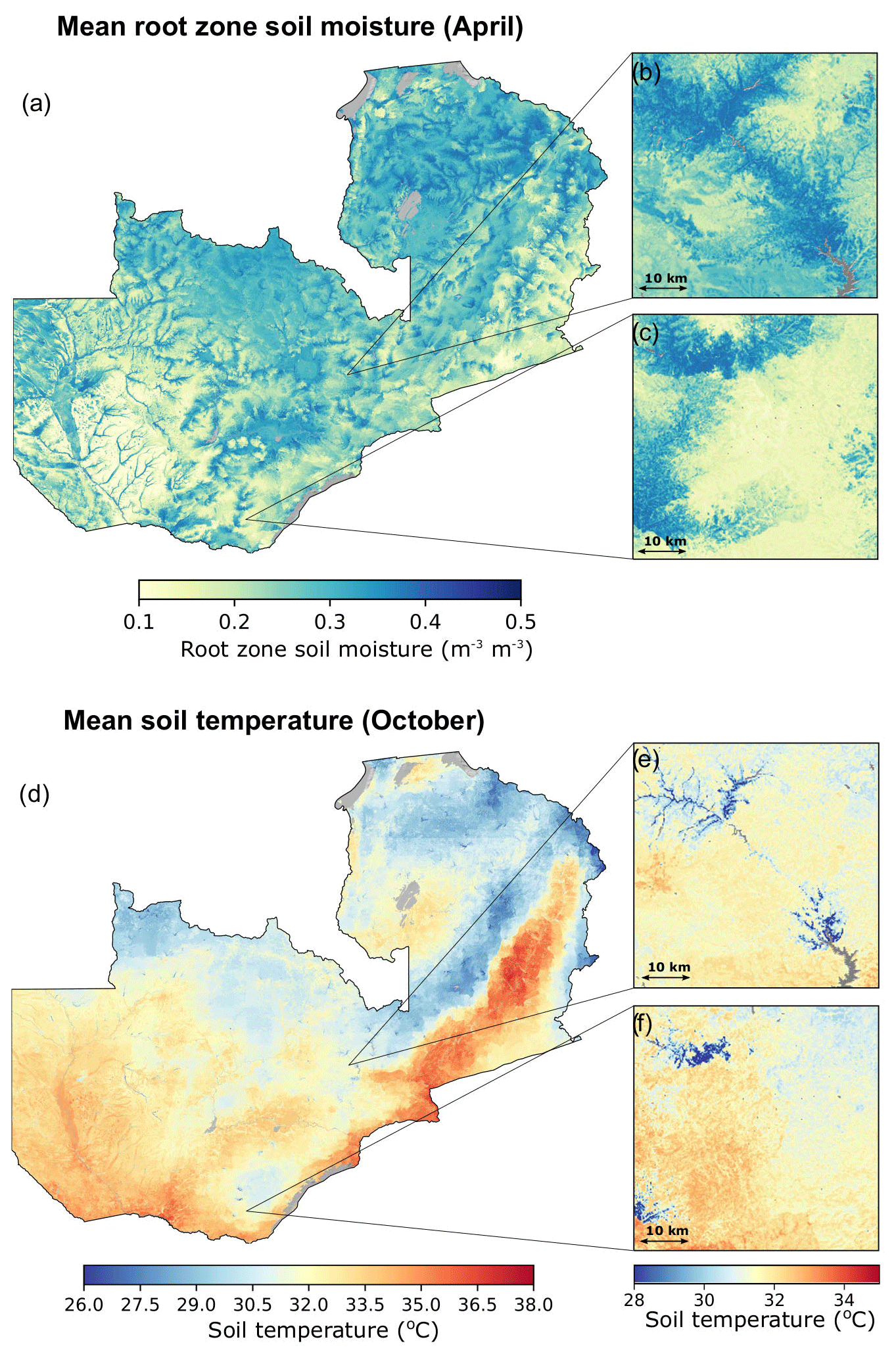
Figure 1April root zone soil moisture and October soil temperature were the most predictive variables in the RF model. Panels (a) and (b) show respective mean values (2000–2018), at the 30 m spatial resolution, as simulated by the HydroBlocks land surface model. Large lakes are excluded from the simulations (gray areas).
3.2 District-level maize yield modeling and importance of predictors
The best-performing RF model was able to predict the values of the district-level yield data, with an average mean absolute error of 310 kg ha−1 and an R2 of 0.57 (year-based cross-validation). Figure 2 shows the comparison between observed and predicted yields for each year (with the model trained on data of all the other years). The model captures the overall patterns of district-level maize yields but with a tendency to underestimate maize yields above 2500 kg ha−1 in the recent years (e.g. 2011–2014) and overestimate low yields in the earlier years (e.g. 2001–2004).
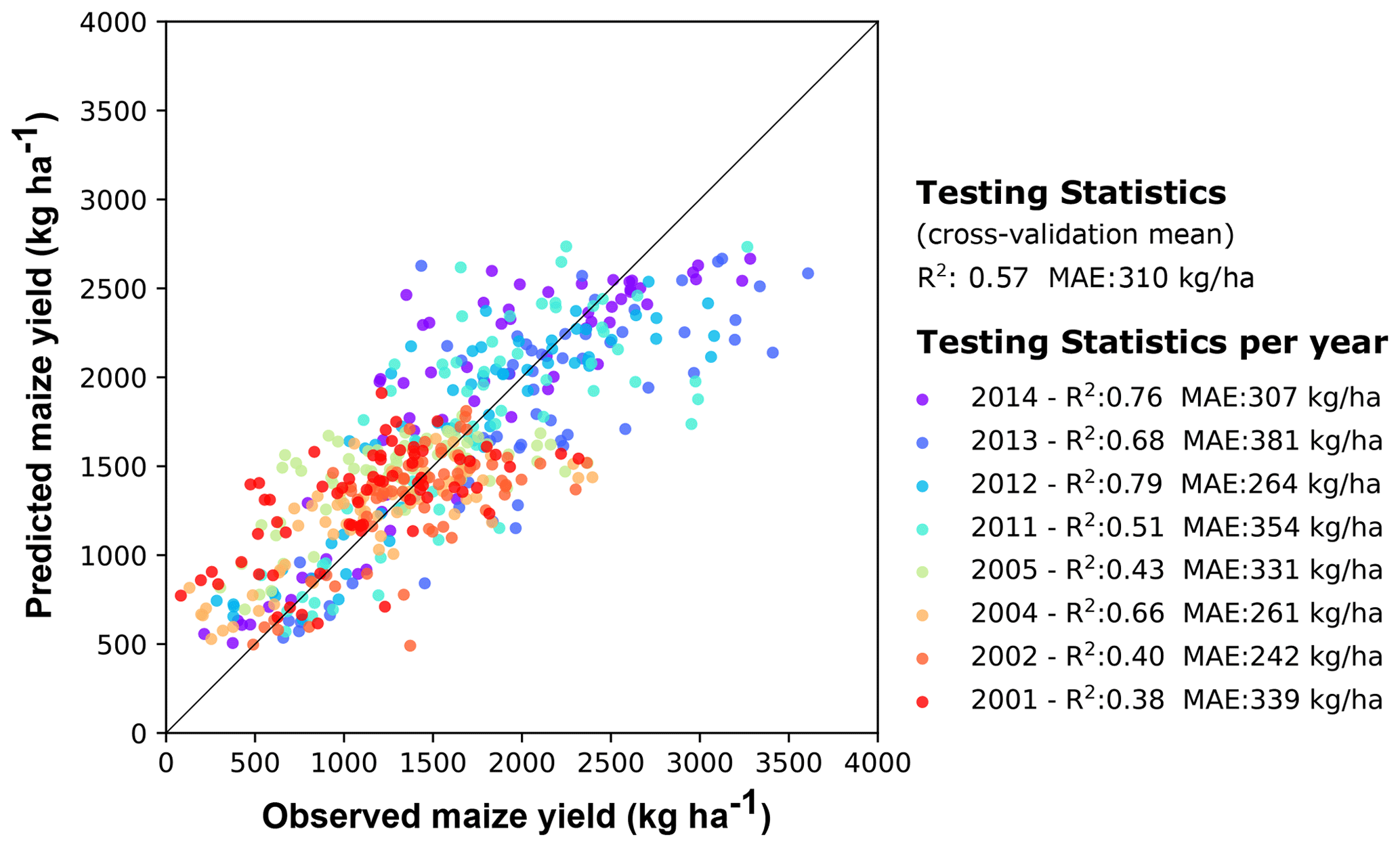
Figure 2Comparison between observed and predicted maize yields at the district scale. The predictions were obtained by training a random forest model with survey-based maize yield data and fine-scale geospatial environmental data sets. Each color shows the maize yield evaluation for a given year (trained on data of the other years).
The recursive feature elimination process, combined with the sensitivity analysis (Table 2), revealed that soil moisture and soil temperature variables were consistently the strongest predictors of yield (Fig. 3). In the first two sensitivity tests, in which Hydroblocks variables were included, soil moisture and temperature variables provided five or six of the top seven predictors, while removing soil moisture and temperature variables as predictors (case 3) resulted in the largest drop in overall model R2 (0.06 and 0.08). On the other hand, removing meteorological variables resulted in relatively little loss of model explanatory power, with an R2 drop of only 0.02 between cases 1 and 2.
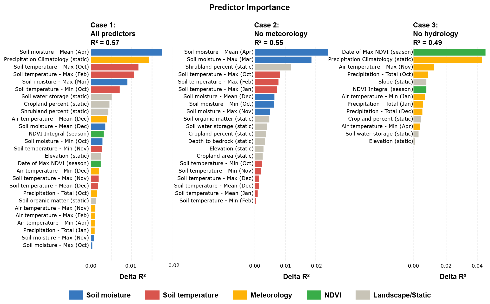
Figure 3The most important predictors for maize yield at the district scale. The predictors were selected and ranked via recursive feature elimination, with the importance rank shown in terms of delta R2. Results are shown for case 1 (considering all the variables), case 2 (without precipitation and air temperature predictors), and case 3 (without soil moisture and soil temperature predictors). Each color represents different categories of predictors data.
In terms of specific variables, cases 1 and 2 both showed that the mean relative soil moisture in April was the strongest predictor of yield, followed by precipitation climatology, October and February soil temperatures, and then March soil moisture (Fig. 3). There are two static variables that appear to have some strong influence as well, namely shrubland percentage, which is ranked third in case 2, and precipitation climatology, which represents the spatial distribution of rainfall, appearing second in case 1 and accounts for an R2 drop of 0.02 if removed from the model. Besides this variable, no other meteorologically derived variable, including all the dynamic measures, ranks highly in the presence of HydroBlocks variables. The highest of these is December mean air temperature, which ranks 10th in case 1. Removing HydroBlocks variables (case 3) increases the influence of these variables, but they still remain less predictive than the static precipitation climatology, while the dynamic vegetation measures, date of maximum NDVI, and the corresponding value are, respectively, the first and sixth most influential. NDVI-derived variables otherwise rank 12th in case 1 and were not retained in case 2.
3.3 Field-scale maize yields for Zambia
At the field scale, RF-predicted maize yields averaged 1557 kg ha−1 (±219 kg ha−1) for the 2000–2018 period. As expected, we observe higher average maize yields in the northern parts of the country and lower average yields in the southern regions (Fig. 4a), which reflects the spatial distribution of mean rainfall. Figure S6 in the Supplement shows time series of the predicted yields for different locations across the country. In terms of the temporal coefficient of variation (Fig. 4d), yield variability is highest in the central, southern, and eastern parts of the country and lowest in northern and northwestern Zambia. In general, there is an inverse relationship between mean annual yields and their coefficient of variation (Fig. S2 in the Supplement); however, there are several notable departures. For example, a landscape-level view in central Zambia reveals areas of moderate to high yields (Fig. 4b) with corresponding moderate to high levels of variability (Fig. 4f), due to proximity to rivers and extensive floodplains, where inundation is frequent. The opposite pattern is seen in southern Zambia, where portions of the landscape show low yields and relatively low variability (Fig. 4c and e) due to more consistently dry conditions.
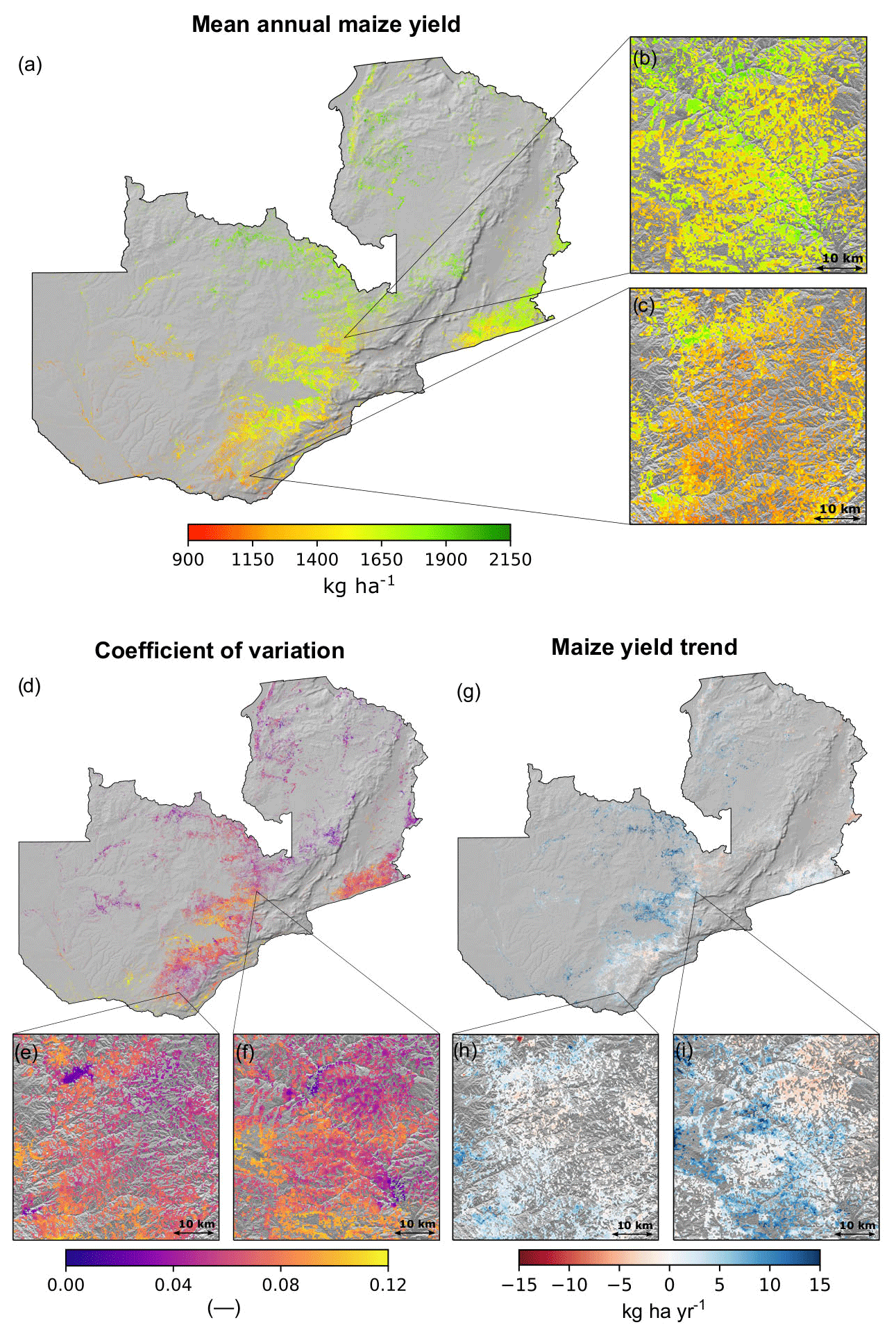
Figure 4Annual maize yields (a), coefficient of variation (d), and maize yield trends (g) for the period between 2000–2018 estimated using a random forest model. Each magnified panel (b, c, e, f, h, i) shows the respective estimates at a 250 m resolution for a 50 km×50 km area.
Analyzing the change in maize yields trends for the period 2000–2018 (Fig. 4g, h, and i), we found that, on the whole, maize productivity increased by 3.5 (±4.6 ). The gain was more prominent in the northern and central parts of the country, particularly in the floodplains (Fig. 4i), rising to 15 , while there was little change in southern Zambia. The productivity also tends to be higher at the locations near floodplains (Fig. 4i). Nonetheless, the overall yield gains rates observed were far behind than the rates required to match the 12 000 kg ha−1 Zambia yield potential (Mueller et al., 2012).
During the 2015–2016 El Niño drought, Zambian agricultural production was severely impacted with overall losses across the country. Our field-scale RF-predicted yields were able to capture these losses (Fig. 5). The countrywide predicted mean yield for 2015–2016 was 1514 kg ha−1 (±233 kg ha−1), which represents an overall loss of 84 kg ha−1 (±60 kg ha−1), or 5.3 %, relative to 2010–2014 mean. Predicted yield reductions were more severe in southern and southeastern Zambia, with losses of 200 kg ha−1 (15 %) across much of this area, reaching as high as 522 kg ha−1 (28 %) (Fig. 5). These estimates align with those of the 20 % losses estimated by the Food and Agriculture Organization (FAO) for this same area during the 2015–2016 El Niño drought (Alfani et al., 2019). However, when evaluating drought impact at the local scales (Fig. 5b and c), we observe that drought impacts yield differently across the landscape. Areas nearby to rivers and floodplains were less prone to crop losses (Fig. 5b), given the wetter and cooler soil moisture conditions.
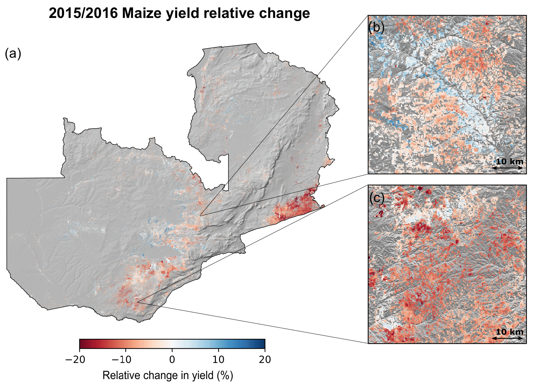
Figure 5(a) Relative change in maize yields (in percent) for the 2015–2016 season with respect to 2010–2014 mean. Each magnified panel (b, c) shows the respective data at a 250 m resolution for a 50 km by 50 km area.
We compared the field-scale yield data aggregated to the district level with the PHS survey district-level yield data. We obtained a Pearson correlation of 0.67 (R2=0.46) and an MAE of 450 kg ha−1. In terms of spatial patterns, aggregated field-scale yield and PHS have a spatial correlation of 0.84. This strong spatial relationship is also evident in the PHS and estimated z scores shown in Fig. S3 in the Supplement. The weak strength and limitations of this aggregated data comparison are discussed in Sect. 4.4.
Field-scale spatial variability of yields and dominant predictors
As observed in Fig. 5b, droughts impact yields differently across the landscape. To quantify to what extent the spatial variability in the hydroclimate and landscape conditions are driving the spatial variability in the yields, we calculated the spatial correlation between the field-scale yields and the dominant predictors (Fig. 6). The spatial correlation was calculated each year, to assess whether these associations changed inter-annually, and over different locations (the entire country and for 50 km×50 km boxes in southern, central, and northern Zambia) to assess how the relationships change regionally.
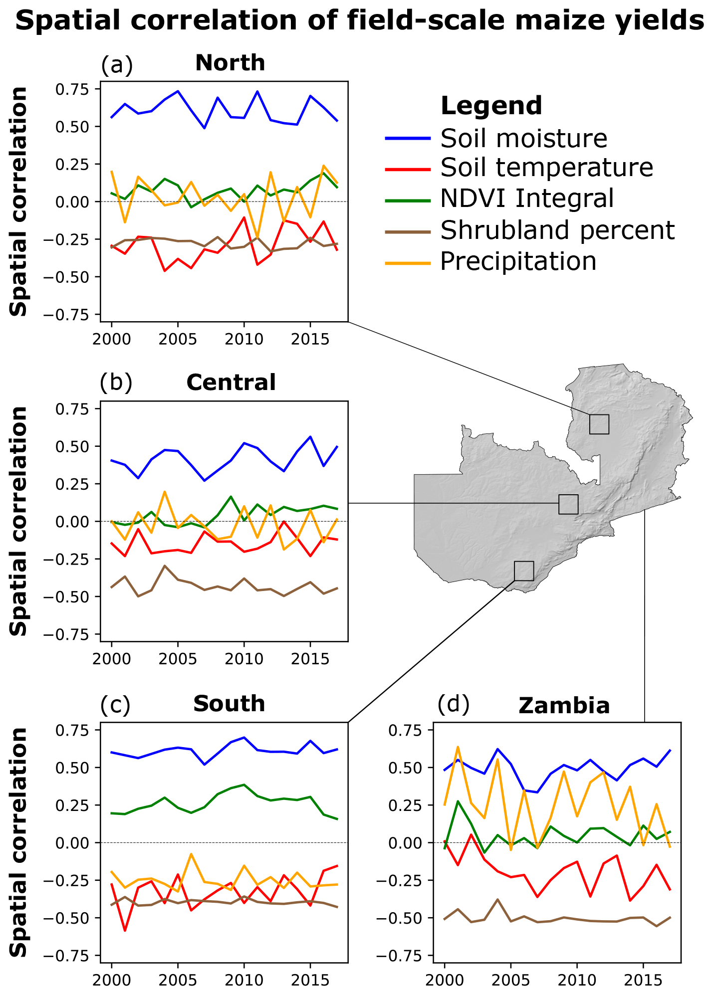
Figure 6Time series of Pearson spatial correlation of maize yields and the most important predictors. Panels show the spatial correlation within 50 km by 50 km boxes in (a) south, (b) central, and (c) north of Zambia. Panel (d) shows the spatial correlation for the entire country.
Soil moisture exhibited the largest impact on the spatial variability in yields, with the highest spatial correlation across all three subregions and the entire country (Fig. 6a–d). Soil temperature and shrubland percent are negatively correlated with yield. The relative ranking and temporal dynamics of the spatial correlations are generally consistent across regions, although the strength of correlation varies between regions, with close to zero correlation for most predictors in the central and northern regions. Given its coarser spatial scale and smoother spatial variability, precipitation climatology showed no spatial correlation with the field-scale yield for each region, but strong correlations at the national scale due to the substantial spatial gradient. However, the high interannual variability indicates the influence of other factors. With the exception of southern Zambia, NDVI showed a low spatial correlation with yield over time.
3.4 The impact of drought on field-scale maize yields
To examine the effectiveness of the six potential drought indicators (Table 3), we evaluated the degree of influence that each indicator had on the anomalies of the predicted field-scale yields (Fig. 7). Overall, the relationship between these indicators and yield anomalies was highly nonlinear. Soil moisture and precipitation percentiles capture the largest yield losses of all six indicators (Fig. 7a and d), with both showing substantial negative anomalies below their 25th percentile values. Yield losses associated with low soil moisture conditions are larger and more certain than those related to low precipitation. For instance, yield losses associated with the 10th soil moisture percentile (202±134 kg ha−1) were 89 % greater than those related to the 10th precipitation percentile (107±135 kg ha−1; orange dashed lines in Fig. 7a and d). At the fifth percentile (red dashed line in Fig. 7a and d), average soil-moisture-related yield loss (235±128 kg ha−1) was 26 % greater than the yield loss associated with the precipitation (187±161 kg ha−1) and, furthermore, had a 20 % narrower confidence interval.
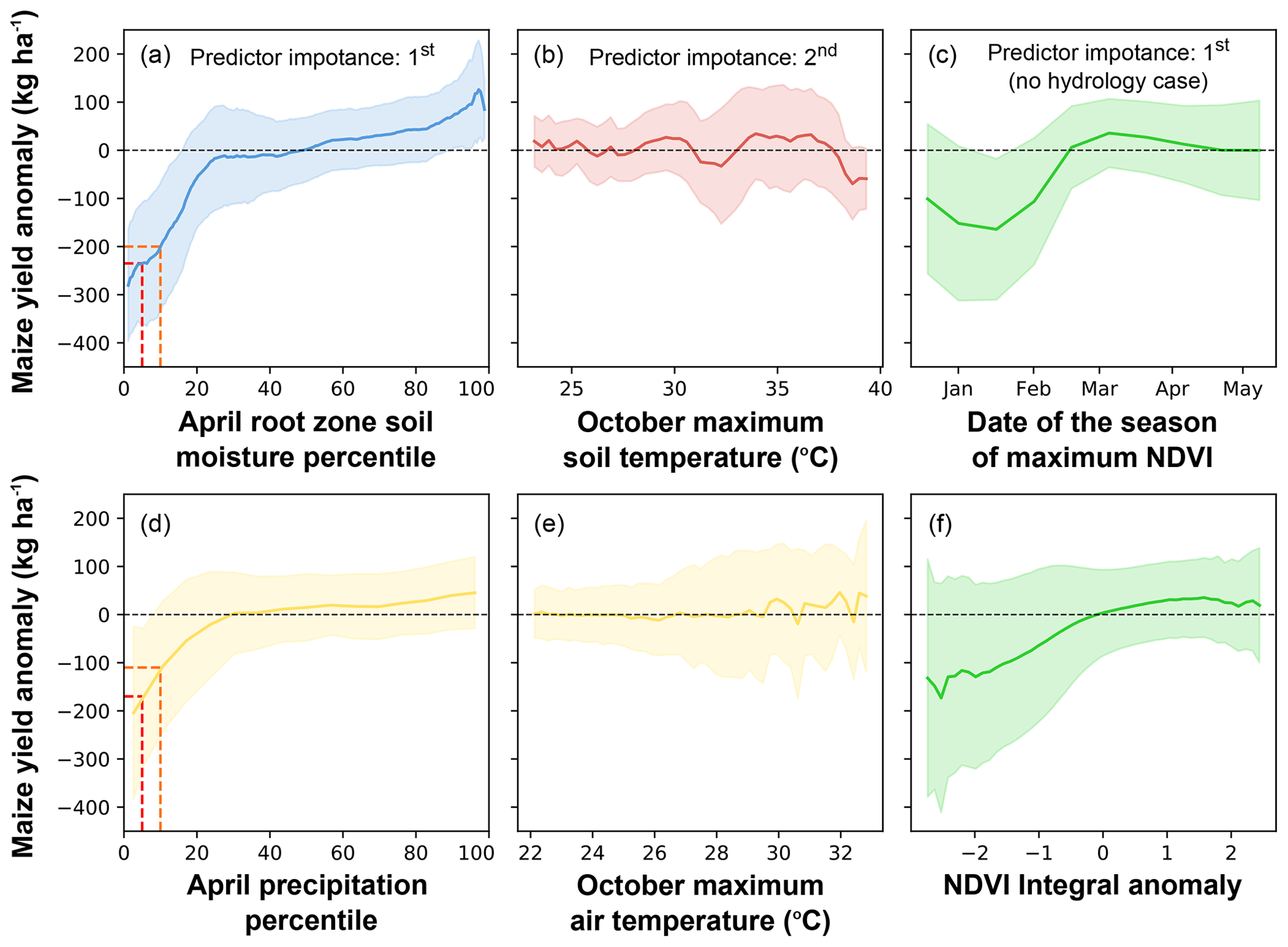
Figure 7The relationship between the field-scale maize yield anomalies with respect to the six drought indicators identified in Table 3. Panels (a–c) show the most predictive variables, and panels (d–f) show the (respective) commonly used variables. Dark lines show the mean values, and shades show the standard deviation. Red and orange dashed lines illustrate potential drought thresholds.
Negative NDVI integral anomaly and early NDVI peak date were also associated with yield reductions (Fig. 7c and f). The strongest and most certain of these was the date of peak NDVI, which resulted in yield anomalies when maximum NDVI occurred before March, with the largest reductions (164±146 kg ha−1) occurring for peak dates between January and February. Negative NDVI integral anomalies also showed substantial but more uncertain yield losses. For example, an NDVI integral anomaly of −2 identified a yield loss of 140±210 kg ha−1.
In contrast to the previous two indicators, there was little variation in yield anomalies associated with soil and air temperature, although the uncertainty in anomalies increased with both measures. However, we observe nearly consistent yield losses with October maximum soil temperatures above 37.5 ∘C, which is near known critical temperature thresholds for maize (Luo, 2011; Schauberger et al., 2017).
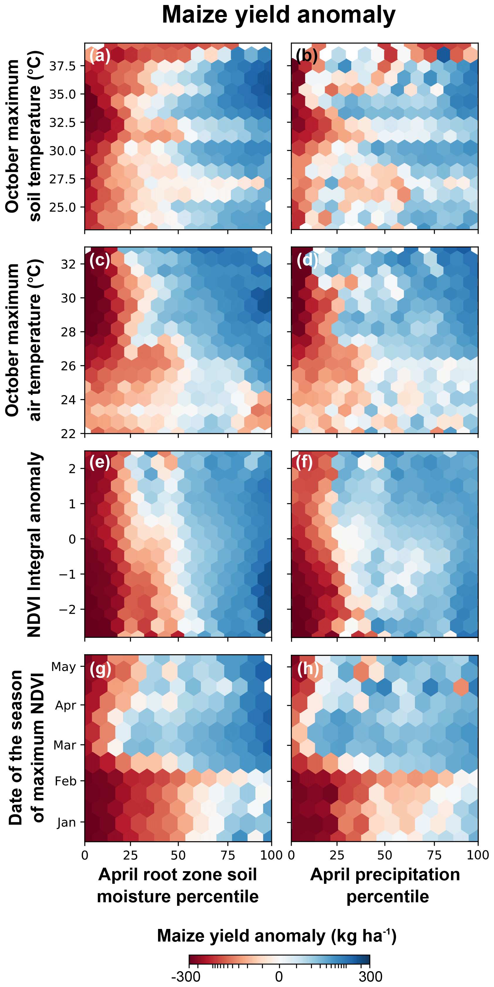
Figure 8Field-scale-estimated maize anomalies as a function of soil moisture and precipitation versus soil temperature, air temperature, date of maximum NDVI, and NDVI integral anomaly. Each hexagon shows the mean yield anomaly, where red (blue) shows overall yield losses (gains). Figure S4 in the Supplement shows the data density of each hexagon.
To gain further insight into the conditions (e.g., hot and dry vs. hot and wet) associated with yield losses, in Fig. 8 we compared how the yield anomalies co-varied with pairwise drought indicators. For example, Fig. 8a shows what the mean yield anomaly associated with its respective October maximum temperature and April root zone soil moisture is. As expected from previous findings (Fig. 7), soil moisture (Fig. 8a, c, and e) and precipitation (Fig. 8b, d, and f) percentiles are the dominant influences on maize yield responses. Both indicators show similar patterns, but the yield responses associated with precipitation are noisier. Extreme soil temperature (Fig. 8a and b) and air temperature (Fig. 8c and d) only lead to yield losses (red) when the soil moisture and precipitation percentiles are low (<25th). High temperatures under wet conditions (top right corners in Fig. 8a–d) show increased productivity (blue). Yield losses occur for the full range of NDVI peak dates when soil moisture and precipitation percentiles are below 10–15th, but when the peak date is earlier than March, yield losses occur when soil moisture and precipitation fall below their median values (Fig. 8g and h). NDVI integral anomalies below zero and below median soil moisture values show a similar relationship with yield (Fig. 8e), but this tendency was much weaker when assessed with precipitation (Fig. 8f).
4.1 Key findings
We presented a modeling framework that combines physically based, hyper-resolution land surface modeling and machine learning for maize yield prediction at the field scale. Our work advances on previous approaches by integrating field-scale hydrological variables into yield prediction and by more effectively quantifying yield sensitivity to drought. Our key findings are as follows:
-
Model skill. The modeling approach that we developed was able to estimate maize yields at district scale with comparable skill (R2=0.57; MAE = 310 kg ha−1) compared to state-of-the-art approaches based on mechanistic yield models (e.g., Jin et al., 2017; Azzari et al., 2017) and with higher skill than standard empirical approaches based on weather variables or vegetation indices (Estes et al., 2013; Zhao et al., 2018).
-
Yield estimates. The field-scale results showed a mean maize yield of 1557 kg ha−1 (±219 kg ha−1) across Zambia, with an overall increasing production trend of 3.5 (±4.6 ) between 2000 and 2018. The field-scale yields captured maize losses during the 2015–2016 El Niño drought at similar levels to losses reported by the FAO based on actual yield data (Alfani et al., 2019).
-
Drivers of yield. We identified soil moisture as the main driver of maize yield variability at both the district scale and field scale. At the district scale, soil moisture was followed in importance by soil temperature, shrubland percent coverage, and precipitation climatology. Time-varying meteorological predictors (precipitation and air temperature) played a minor role. NDVI-based predictors only showed meaningful contribution when soil moisture and soil temperature predictors were absent.
-
Drought impacts. There is a highly nonlinear behavior between drought indices and yield losses. However, consistent maize losses are observed when soil moisture or precipitation drop below the 25th percentile. At extreme dry conditions (fifth percentile), soil moisture identifies 26 % more losses with 21 % less uncertainty than precipitation, providing an effective measure of drought impact. Significant yield losses are also predicted when soil temperature exceeded 37.5 ∘C in the early growing season. Drought impacted yields differently across the landscape (Fig. 5), with most of the spatial variability coming from soil moisture (Fig. 6).
4.2 Drivers of maize yields predictability
Soil moisture and precipitation
Soil moisture and soil temperature showed a strong contribution to yield prediction because they represent the water and temperature balances at the root zone, accounting for the soil–water–plant interactions via infiltration, surface and subsurface flow, vertical drainage, water uptake by plants, and evaporation. Consequently, in our sensitivity experiments, in case 1 and case 2, the meteorological predictors added only minor improvements to yield prediction beyond the contribution of root zone predictors, mainly because precipitation does not necessarily translate into water availability for plants. For example, rainfall from intense storms may contribute mostly to runoff rather than infiltration, leading to a spatial mismatch between where the water is supplied (precipitation) and where water is finally available to plants (soil moisture). Furthermore, whilst temperature drives the atmospheric demand for evapotranspiration, it does not reflect the complexity of controls on transpiration, which are more water limited (rather than energy limited) in drier regions such as much of Zambia (Berg et al., 2016; Williams et al., 2012; McNaughton and Jarvis, 1991).
Distinctions between atmospheric and root zone processes are particularly important at the field scale, due to different natural scales of variability that influence crops in different ways. Precipitation and air temperature operate mostly at larger scales, with most of the spatiotemporal variability coming from large-scale atmospheric circulation and large-scale topographic features (Grayson and Blöschl, 2001). Soil moisture, on the other hand, operates at multiple scales, influenced by the meteorological conditions, but with most of the spatial variability coming from the heterogeneity of the landscape (topography, soil properties, and land cover; Crow et al., 2012; Famiglietti et al., 2008; Grayson and Blöschl, 2001). By providing soil moisture and soil temperature estimates at a spatial scale closer to its natural scale of variability, HydroBlocks allows for improved yield predictions. This is indicated by comparison of the joint distribution of soil moisture and precipitation percentiles (Fig. 9), which shows that most of the time their condition will be similar (0.78 correlation), yet when they are different (due to the above reasons), soil moisture better captures losses in yield.
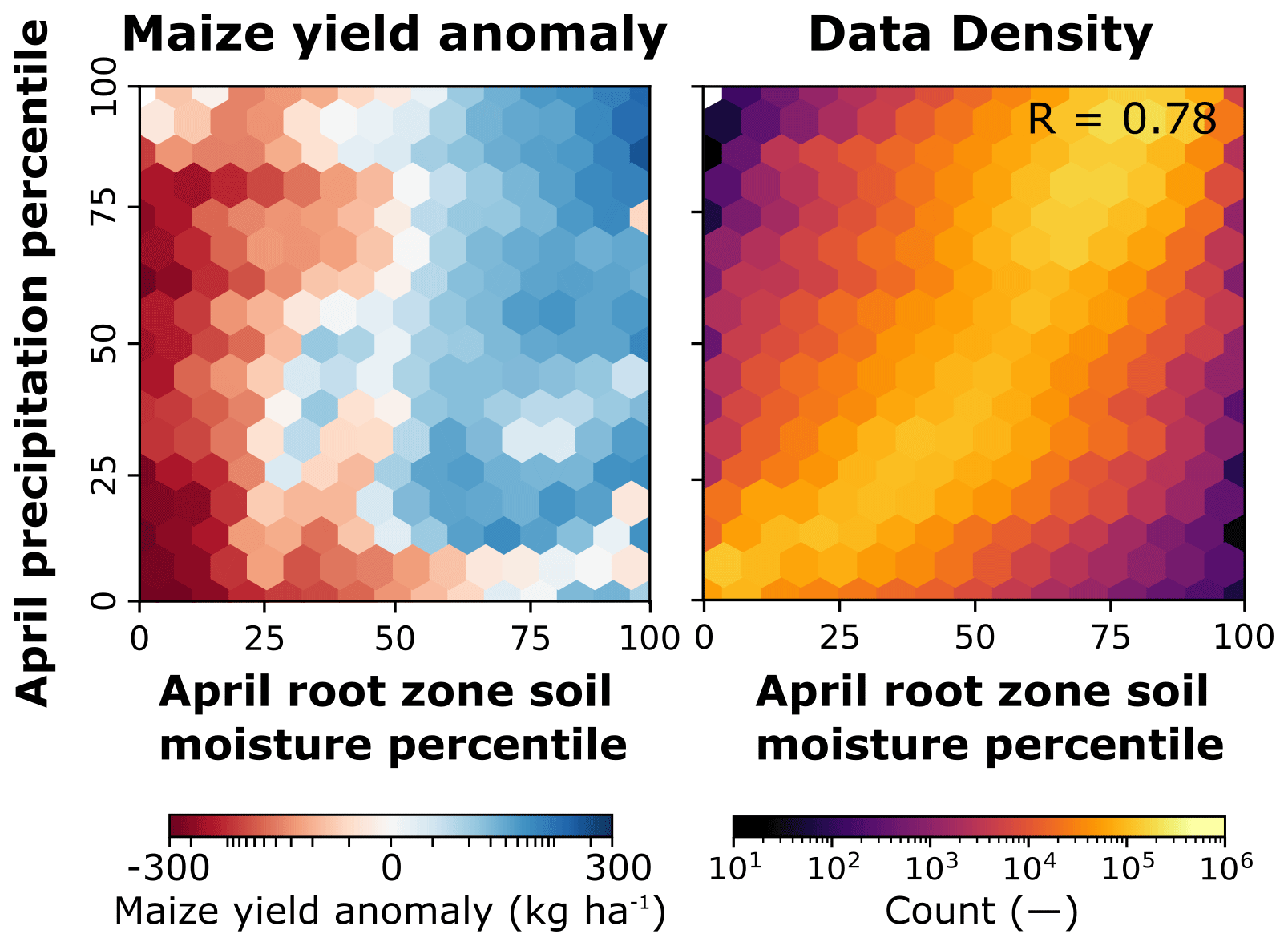
Figure 9Mean maize anomalies and data density as a function of root zone soil moisture and precipitation percentiles.
April soil moisture ranked as the strongest predictor of yield. April covers the grain-filling stage of the maize calendar in Zambia (∼35 d prior to maturity; Yonts et al., 2008), when soil moisture is critical for plants because of the large water uptake demands (Yonts et al., 2008; Borras et al., 2003). Despite the high greenness of the season (measured by vegetation indices such as NDVI, for example), if plants do receive enough water in the reproductive period, then the cob will not develop well, compromising productivity. Although several studies identified NDVI as the strongest predictors for maize (Table 1 in Funk and Budde, 2009; Johnson, 2016; Petersen, 2018; Karthikeyan et al., 2020), our sensitivity analysis results (Fig. 3; case 3) showed that only in the absence of soil moisture and soil temperature variables do NDVI-based variables emerge as strong predictors of yield. This is evident in Fig. 8e and g, which show that NDVI-based anomalies have little sensitivity to change in yields when compared to soil moisture. This could also be a limitation of visible satellite sensors in capturing under canopy plant–soil–water dynamics. A further discussion on NDVI limitations is presented in Sect. 4.4.
Soil temperature and extreme heat
Soil temperatures in October (sowing period) are also critical for controlling yields. When the rainy season is delayed, extreme temperatures in the early stages can potentially damage seeds prior to their germination (Mulenga et al., 2016) or cause an earlier start to the maize reproductive period, increasing the susceptibility to heat and water stress (Harrison et al., 2011; Hatfield and Prueger, 2015). However, elevated temperatures in the early season only lead to yield losses when the soil moisture content at the end of the season was low; otherwise, an overall yield gain is observed (Fig. 8a). Thus, wet soil moisture conditions (e.g., irrigation) could play an important role in mitigating extreme heat effects (Troy et al., 2015; Thomas et al., 2020) and potentially even increase productivity (Steward et al., 2018), such as observed in Fig. 5b. Nonetheless, because of maize's overall sensitivity to elevated temperatures (Lobell and Field, 2007; Lobell et al., 2013), soil temperature above 37.5 ∘C would lead to yield losses despite the wet conditions in the late season (Fig. 8a and b).
Static landscape predictors
In terms of the static predictors, shrubland ranked third in case 2 as it may represent the heterogeneity of agricultural landscapes. While high cropland percent could be associated with more homogenous agricultural fields (often associated with commercial farming), high shrubland percent may indicate a higher presence of fragmented agricultural areas, reflecting poorer agricultural landscapes (from a physical and management perspective) and, consequently, lower yields (Maggio et al., 2018). Figure S5 in the Supplement illustrates this relationship. On the other hand, actual shrubland/cropland mosaics may be more likely to be misclassified as a cropland pixel (commission error), which could explain the negative influence that shrubland percent has on yield. Landscape characteristics, such as slope and properties of the soil (residual soil moisture, soil water storage capacity, and wilting point), were also identified as important predictors. These predictors control soil moisture dynamics and the water-holding capacity of the soil, as more water available from plants for longer increases the likelihood of higher yields.
Climatologically based predictors
Climatological precipitation over the growing season also ranked as a strong predictor, as it represents the mean spatial distribution of rainfall. Historically, yields in Zambia are higher in locations with more precipitation during the growing season (Zhao et al., 2018). On the other hand, in the RFE analysis, monthly precipitation (i.e., dynamic) only ranked 10th. This could be because soil moisture dominated the predictive power at the subannual timescale but also because of the spatial scale mismatch between the input data (30 m soil moisture, 1 km climatological precipitation, and 9 km dynamic precipitation predictors). Conversely, climatological air temperature over the growing season did not remain after RFE, but monthly air temperatures in the early season showed predictive importance, highlighting its contribution at subannual timescales.
4.3 Drivers of maize yield spatial variability
Our results show that there is large spatial variability in yields at national and local scales (Fig. 4) that is consistently and mainly driven by the spatial variability in soil moisture (Fig. 6). The spatial variability in soil moisture originates from the interactions between the meteorological conditions and the landscape. For instance, topography controls lateral flows at the root zone, driving the wet (Fig. 1b) and cooler (Fig. 1e) soil conditions at the river valleys. Soil properties also influence the spatial variability in soil moisture by driving soil moisture dynamics (e.g., infiltration rates) but also thermal properties of the soil (e.g., thermal conductivity). Land cover and vegetation types (Fig. S1) control land–atmosphere interactions (i.e., evapotranspiration), water retention in the root zone, and surface runoff processes. This spatial variability in hydroclimate processes, along with the different farmer management practices, leads to different drought impacts on yields across the landscape. This is evident in the 2015–2016 El Niño drought. Figure 5a and b show that, despite the severity of the event, areas frequently wet and cooler at river valleys are less prone to agriculture losses. If this modeling framework was implemented using coarser hydrological data, we do not expect significant changes in the RF performance (as the data is aggregated to the district level for training), but we do expect a smoother field-scale yield prediction. This is expected because hydrology plays an important role in the spatial patterns of the predicted yields, as soil moisture and soil temperature were the strongest predictors (Fig. 3). This spatial variability in the impact of drought on yields has important implications for decision-making (at national and local scales) as traditional coarse-scale drought indices (and aggregated yield surveys) would have only captured averaged impacts, likely missing the extremes. However, future research should further evaluate the role of spatial scaling in field-scale yield predictions.
4.4 Challenges and limitations for field-scale maize yield prediction
Extending the RF model to predict maize yields at the field scale is done under the assumption that the model predictors and parameters trained at the district scale reflect the relationships at the field scale. However, there are uncertainties in the training data, predictors, and model parameters that lead to uncertainties in district-level and field-scale-level maize yield estimates. There are also uncertainties in how yields vary at small scales and the physical processes and variability in management that drive this.
Maize yield training data
The PHS survey-based data set, used to train the RF model, was computed by aggregating individual farmer self-reported harvest (number of maize bags) and field areas to the district level. While aggregating the data provides a more reliable estimate of yield, as it smooths out the noise and removes outliers, it also constrains the ability of the model to predict high and low yields. Similarly, self-reported, field-scale data are also very uncertain and sensitive to errors when estimating yields (harvest/area; Paliwal and Jain, 2020; Gourlay et al., 2019). Ideally, to improve the capability of modeling yield extremes and to ensure the reliability of the field-scale yield estimates, models should be trained on yield data that was properly measured (in terms of weight and area). Currently, such data are hard to obtain for Zambia (and other countries in the region), except for field trials and focused research projects. However, by assuming that the RF model trained on district-level data can reflect the major drivers of maize yields, we provide an estimate of field-scale yield variability that is, at least, grounded in reliable district-level estimates. Comparing and validating field-scale yield estimates is also challenging, mainly because of the mismatches between survey-observed and model-estimated yields. For instance, we assume that the PHS survey (district-level yield data) is representative of the overall yield at each district (i.e., there were no survey sampling issues) and that all 250 m grid cells with at least 50 % cropland were maize fields. These mismatches may lead to biases in the aggregated-level estimates.
Modeling framework and predictors
Despite the good potential to predict yields, our yield predictions showed a tendency to underestimate high yields (>2500 kg ha−1) and slightly overestimate low yields (<500 kg ha−1), as observed in Fig. 2. This could be due to the above reasons but also due to the limited training data of extreme high and low values and a consequence of the RF model being somewhat limited in predicting extreme values, as its final estimates are an average of an ensemble of decision trees (e.g., Baccini et al., 2004; Bourgoin et al., 2018). The underestimation of high yields could also be associated with the lack of information on farmer management, such as the use of drought-resistant seeds, fertilizers, or irrigation systems, that are not accounted for in the model. The human-driven factors can play a major role in modulating yield outcomes, especially when hydroclimate conditions are not favorable. We expected vegetation-index-based predictors to improve the capability of the model to identify high yields; however, NDVI only ranked 12th on the RFE (<0.005 change in R2; Fig. 3). This could be attributed to mixed NDVI signals from other crops (as we only map cropland occurrence and not maize occurrence), infrequent retrievals (biweekly) with high cloud coverage, and the NDVI tendency to saturate at high LAI values. We also expected socioeconomic-based predictors, such as GDP and population, to reflect farmers' access to technology, infrastructure, and markets. However, these predictors were removed by the RFE analysis, showing that yields were not influenced by these socioeconomic variables (similar to Jain, 2007) but mostly influenced by early season temperature and mid–late season rainfall.
In addition, the uncertainties associated with the strongest predictors could be also reflected in uncertainties in the maize yield prediction. As most of the temporal and spatial variability in yields comes from the variability in soil moisture and soil temperature (Fig. 6), considering the uncertainties from these estimates is fundamental. Uncertainties arise mostly from LSM input data such as soil properties, meteorological conditions, and land cover, as well as model parameterizations. While validation allows us to quantify the reliability of the simulation, in situ observations are nonexistent in most of the developing world. Given that agricultural yield dynamics are also heavily influenced by human intervention, pathways forward should consider predictors that better account for human management of crop yields. This can be achieved by accounting for water resources management (e.g., irrigation) when modeling soil moisture dynamics but also by including additional predictors that reflect farmer decision-making (e.g., information on planting dates, seed and varietal choice, use of pesticides, fertilizers, and machinery, etc.).
Current drought monitoring often relies on hydroclimate data at coarse spatial resolutions or (infrequent) vegetation index retrievals that do not always indicate the conditions farmers face in the field. As a result, few studies were able to link drought indices to agricultural losses in the field (Karthikeyan et al., 2020; Sutanto et al., 2019). Consequently, decision-making (by governments and policy-makers, insurance payouts, water resources management, etc.) based on these indices can often be disconnected from the farmers' reality.
With the advancement of hyper-resolution modeling (Wood et al., 2011; Bierkens et al., 2014; Chaney et al., 2016; Vergopolan et al., 2020), a new paradigm has been established that allows field-scale agricultural prediction and drought monitoring. In this work, this is achieved by accounting for the water balance in the root zone as a critical variable for crop productivity and by representing soil moisture and soil temperature dynamics at a scale that is representative of farm-scale spatial variability. In specific, we used the HydroBlocks model to estimate 30 m soil moisture and soil temperature (1981–2018) and combine these and other predictors with random forests to model and map 250 m maize yields (2000–2018) across Zambia. To our knowledge, this study is the first to estimate historical field-scale soil moisture and temperature in this region. Our work advances on previous approaches by integrating these variables into yield prediction and by more effectively quantifying yield sensitivity to drought at the smallholder farm scale.
By bridging the spatial-scale gap between drought monitoring and field-scale agricultural impacts, this work paves the way towards applying field-scale soil moisture monitoring to inform agricultural decision-making across scales. Although our approach is complex and involves integrating remote sensing data, hyper-resolution land surface modeling, long-term district level yield data, and machine learning, it can provide the basis for a practical approach to field-scale monitoring that is an improvement on current approaches that are less accurate and at a coarse resolution. In addition, it complements and can help to minimize the difficult task of collecting field-based yield data, which is one of the primary limitations for remote agricultural impact assessments. At the same time, accurate field-scale yield data and information on biophysical parameters (e.g., soils) and farmer-level management practices are still needed to improve and further validate the approach.
The data that support the findings of this study are available on request from the corresponding author.
The supplement related to this article is available online at: https://doi.org/10.5194/hess-25-1827-2021-supplement.
NV, LE, and JS conceived the research. NV designed and performed the analysis, with support from SX in the modeling and mapping of maize yields. JS, LE, and EFW were responsible for the funding acquisition. NV led the writing of the paper, and all co-authors provided critical feedback and contributed to the writing of the paper.
The authors declare no competing interests.
This research has been supported by the National Science Foundation (grant no. 1832393) and the National Aeronautics and Space Administration (grant nos. NNX14AH92G and 80NSSC18K0158).
This paper was edited by Lixin Wang and reviewed by Hannah Kerner and Karthikeyan Lanka.
Adegoke, J. O. and Carleton, A. M.: Relations between Soil Moisture and Satellite Vegetation Indices in the U.S. Corn Belt, J. Hydrometeorol., 3, 395–405, https://doi.org/10.1175/1525-7541(2002)003<0395:rbsmas>2.0.co;2, 2002. a
Aghighi, H., Azadbakht, M., Ashourloo, D., Shahrabi, H. S., and Radiom, S.: Machine Learning Regression Techniques for the Silage Maize Yield Prediction Using Time-Series Images of Landsat 8 OLI, IEEE J. Sel. Top. Appl., 11, 4563–4577, https://doi.org/10.1109/jstars.2018.2823361, 2018. a
Alfani, F., Arslan, A., McCarthy, N., Cavatassi, R., and Sitko, N.: Climate-change vulnerability in rural Zambia: the impact of an El Niño-induced shock on income and productivity, available at: http://www.fao.org/3/ca3255en/CA3255EN.pdf (last access: 18 May 2020), 2019. a, b, c, d
Archer, K. J. and Kimes, R. V.: Empirical characterization of random forest variable importance measures, Comput. Stat. Data An., 52, 2249–2260, https://doi.org/10.1016/j.csda.2007.08.015, 2008. a, b
Azzari, G., Jain, M., and Lobell, D. B.: Towards fine resolution global maps of crop yields: Testing multiple methods and satellites in three countries, Remote Sens. Environ., 202, 129–141, https://doi.org/10.1016/j.rse.2017.04.014, 2017. a, b
Baccini, A., Friedl, M. A., Woodcock, C. E., and Warbington, R.: Forest biomass estimation over regional scales using multisource data, Geophys. Res. Lett., 31, L10501, https://doi.org/10.1029/2004gl019782, 2004. a
Bachmair, S., Svensson, C., Hannaford, J., Barker, L. J., and Stahl, K.: A quantitative analysis to objectively appraise drought indicators and model drought impacts, Hydrol. Earth Syst. Sci., 20, 2589–2609, https://doi.org/10.5194/hess-20-2589-2016, 2016. a
Bank, T. W.: Global Risk Data Platform: Gross Domestic Product. United Nations Environment Programme, available at: http://preview.grid.unep.ch/ (last access: 10 June 2019), 2012. a
Beck, H. E., Pan, M., Miralles, D. G., Reichle, R. H., Dorigo, W. A., Hahn, S., Sheffield, J., Karthikeyan, L., Balsamo, G., Parinussa, R. M., van Dijk, A. I. J. M., Du, J., Kimball, J. S., Vergopolan, N., and Wood, E. F.: Evaluation of 18 satellite- and model-based soil moisture products using in situ measurements from 826 sensors, Hydrol. Earth Syst. Sci., 25, 17–40, https://doi.org/10.5194/hess-25-17-2021, 2021. a
Berg, A., Findell, K., Lintner, B., Giannini, A., Seneviratne, S. I., van den Hurk, B., Lorenz, R., Pitman, A., Hagemann, S., Meier, A., Cheruy, F., Ducharne, A., Malyshev, S., and Milly, P. C. D.: Land–atmosphere feedbacks amplify aridity increase over land under global warming, Nat. Clim. Change, 6, 869–874, https://doi.org/10.1038/nclimate3029, 2016. a
Beza, E., Silva, J. V., Kooistra, L., and Reidsma, P.: Review of yield gap explaining factors and opportunities for alternative data collection approaches, Eur. J. Agron., 82, 206–222, https://doi.org/10.1016/j.eja.2016.06.016, 2017. a
Bierkens, M. F. P., Bell, V. A., Burek, P., Chaney, N., Condon, L. E., David, C. H., de Roo, A., Döll, P., Drost, N., Famiglietti, J. S., Flörke, M., Gochis, D. J., Houser, P., Hut, R., Keune, J., Kollet, S., Maxwell, R. M., Reager, J. T., Samaniego, L., Sudicky, E., Sutanudjaja, E. H., van de Giesen, N., Winsemius, H., and Wood, E. F.: Hyper-resolution global hydrological modelling: what is next?, Hydrol. Process., 29, 310–320, https://doi.org/10.1002/hyp.10391, 2014. a
Borras, L., Westgate, M. E., and Oteguie, M. E.: Control of kernel weight and kernel water relations by Post-flowering Source–sink ratio in maize, Ann. Bot.-London, 91, 857–867, https://doi.org/10.1093/aob/mcg090, 2003. a
Bourgoin, C., Blanc, L., Bailly, J.-S., Cornu, G., Berenguer, E., Oszwald, J., Tritsch, I., Laurent, F., Hasan, A., Sist, P., and Gond, V.: The Potential of Multisource Remote Sensing for Mapping the Biomass of a Degraded Amazonian Forest, Forests, 9, 303, https://doi.org/10.3390/f9060303, 2018. a
Breiman, L.: Random Forests, Mach. Learn., 45, 261–277, https://doi.org/10.1023/a:1017934522171, 2001. a, b
Cai, X., Pan, M., Chaney, N. W., Colliander, A., Misra, S., Cosh, M. H., Crow, W. T., Jackson, T. J., and Wood, E. F.: Validation of SMAP soil moisture for the SMAPVEX15 field campaign using a hyper-resolution model, Water Resour. Res., 53, 3013–3028, https://doi.org/10.1002/2016wr019967, 2017. a
Chaney, N. W., Metcalfe, P., and Wood, E. F.: HydroBlocks: a field-scale resolving land surface model for application over continental extents, Hydrol. Process., 30, 3543–3559, https://doi.org/10.1002/hyp.10891, 2016. a, b, c
Chaney, N. W., Van Huijgevoort, M. H. J., Shevliakova, E., Malyshev, S., Milly, P. C. D., Gauthier, P. P. G., and Sulman, B. N.: Harnessing big data to rethink land heterogeneity in Earth system models, Hydrol. Earth Syst. Sci., 22, 3311–3330, https://doi.org/10.5194/hess-22-3311-2018, 2018. a, b
Chen, J., Jönsson, P., Tamura, M., Gu, Z., Matsushita, B., and Eklundh, L.: A simple method for reconstructing a high-quality NDVI time-series data set based on the Savitzky–Golay filter, Remote Sens. Environ., 91, 332–344, https://doi.org/10.1016/j.rse.2004.03.014, 2004. a
Chen, Y., Lu, D., Moran, E., Batistella, M., Dutra, L. V., Sanches, I. D., da Silva, R. F. B., Huang, J., Luiz, A. J. B., and de Oliveira, M. A. F.: Mapping croplands, cropping patterns, and crop types using MODIS time-series data, Int. J. Appl. Earth Obs., 69, 133–147, https://doi.org/10.1016/j.jag.2018.03.005, 2018. a
Chlingaryan, A., Sukkarieh, S., and Whelan, B.: Machine learning approaches for crop yield prediction and nitrogen status estimation in precision agriculture: A review, Comput. Electron. Agr., 151, 61–69, https://doi.org/10.1016/j.compag.2018.05.012, 2018. a, b
CIESIN: Gridded Population of the World, Version 4 (GPWv4): Population Density, Revision 10, https://doi.org/10.7927/H4DZ068D, 2017. a
Crow, W. T., Kumar, S. V., and Bolten, J. D.: On the utility of land surface models for agricultural drought monitoring, Hydrol. Earth Syst. Sci., 16, 3451–3460, https://doi.org/10.5194/hess-16-3451-2012, 2012. a, b
Deines, J. M., Kendall, A. D., and Hyndman, D. W.: Annual Irrigation Dynamics in the U. S. Northern High Plains Derived from Landsat Satellite Data, Geophys. Res. Lett., 44, 9350–9360, https://doi.org/10.1002/2017gl074071, 2017. a
D'Odorico, P. and Bhattachan, A.: Hydrologic variability in dryland regions: impacts on ecosystem dynamics and food security, Philos. T R. Soc. B, 367, 3145–3157, https://doi.org/10.1098/rstb.2012.0016, 2012. a
Donaldson, D. and Storeygard, A.: The View from Above: Applications of Satellite Data in Economics, J. Econ. Perspect., 30, 171–198, https://doi.org/10.1257/jep.30.4.171, 2016. a
Economist: ARC's covenant, available at: https://www.economist.com/finance-and-economics/2016/08/25/arcs-covenant (last access: 10 June 2019), 2016. a
Enenkel, M., Farah, C., Hain, C., White, A., Anderson, M., You, L., Wagner, W., and Osgood, D.: What Rainfall Does Not Tell Us – Enhancing Financial Instruments with Satellite-Derived Soil Moisture and Evaporative Stress, Remote Sens.-Basel, 10, 1819, https://doi.org/10.3390/rs10111819, 2018. a
Estel, S., Kuemmerle, T., Levers, C., Baumann, M., and Hostert, P.: Mapping cropland-use intensity across Europe using MODIS NDVI time series, Environ. Res. Lett., 11, 024015, https://doi.org/10.1088/1748-9326/11/2/024015, 2016. a
Estes, L. D., Bradley, B. A., Beukes, H., Hole, D. G., Lau, M., Oppenheimer, M. G., Schulze, R., Tadross, M. A., and Turner, W. R.: Comparing mechanistic and empirical model projections of crop suitability and productivity: implications for ecological forecasting, Global Ecol. Biogeogr., 22, 1007–1018, https://doi.org/10.1111/geb.12034, 2013. a
Famiglietti, J. S., Ryu, D., Berg, A. A., Rodell, M., and Jackson, T. J.: Field observations of soil moisture variability across scales, Water Resour. Res., 44, W01423, https://doi.org/10.1029/2006wr005804, 2008. a
FAO: 2015–2016 El Niño Early action and response for agriculture, food security and nutrition (Update 6), available at: http://www.fao.org/fileadmin/user_upload/emergencies/docs/FAOEl%20NinoReportMarch2016.pdf (last access: 18 May 2020), 2016a. a
FAO: 2015–2016 El Niño Early action and response for agriculture, food security and nutrition (Update 10), available at: http://www.fao.org/3/a-i6049e.pdf (last access: 18 May 2020), 2016b. a
Farr, T. G., Rosen, P. A., Caro, E., Crippen, R., Duren, R., Hensley, S., Kobrick, M., Paller, M., Rodriguez, E., Roth, L., Seal, D., Shaffer, S., Shimada, J., Umland, J., Werner, M., Oskin, M., Burbank, D., and Alsdorf, D.: The Shuttle Radar Topography Mission, Rev. Geophys., 45, RG2004, https://doi.org/10.1029/2005rg000183, 2007. a, b
Fick, S. E. and Hijmans, R. J.: WorldClim 2: new 1-km spatial resolution climate surfaces for global land areas, Int. J. Climatol., 37, 4302–4315, https://doi.org/10.1002/joc.5086, 2017. a
Folberth, C., Baklanov, A., Balkovič, J., Skalský, R., Khabarov, N., and Obersteiner, M.: Spatio-temporal downscaling of gridded crop model yield estimates based on machine learning, Agr. Forest Meteorol., 264, 1–15, https://doi.org/10.1016/j.agrformet.2018.09.021, 2019. a, b
Franz, T. E., Pokal, S., Gibson, J. P., Zhou, Y., Gholizadeh, H., Tenorio, F. A., Rudnick, D., Heeren, D., McCabe, M., Ziliani, M., Jin, Z., Guan, K., Pan, M., Gates, J., and Wardlow, B.: The role of topography, soil, and remotely sensed vegetation condition towards predicting crop yield, Field Crop. Res., 252, 107788, https://doi.org/10.1016/j.fcr.2020.107788, 2020. a, b
Funk, C. and Budde, M. E.: Phenologically-tuned MODIS NDVI-based production anomaly estimates for Zimbabwe, Remote Sens. Environ., 113, 115–125, https://doi.org/10.1016/j.rse.2008.08.015, 2009. a
Gourlay, S., Kilic, T., and Lobell, D. B.: A new spin on an old debate: Errors in farmer-reported production and their implications for inverse scale – Productivity relationship in Uganda, J. Dev. Econ., 141, 102376, https://doi.org/10.1016/j.jdeveco.2019.102376, 2019. a, b
Grayson, R. and Blöschl, G.: Spatial patterns in catchment hydrology: observations and modelling, Cambridge Univ. Press, Cambridge, UK, 2001. a, b
Gregorutti, B., Michel, B., and Saint-Pierre, P.: Correlation and variable importance in random forests, Stat. Comput., 27, 659–678, https://doi.org/10.1007/s11222-016-9646-1, 2016. a
Gu, Y., Wylie, B. K., Howard, D. M., Phuyal, K. P., and Ji, L.: NDVI saturation adjustment: A new approach for improving cropland performance estimates in the Greater Platte River Basin, USA, Ecol. Indic., 30, 1–6, https://doi.org/10.1016/j.ecolind.2013.01.041, 2013. a
Guilpart, N., Grassini, P., van Wart, J., Yang, H., van Ittersum, M. K., van Bussel, L. G. J., Wolf, J., Claessens, L., Leenaars, J. G. B., and Cassman, K. G.: Rooting for food security in Sub-Saharan Africa, Environ. Res. Lett., 12, 114036, https://doi.org/10.1088/1748-9326/aa9003, 2017. a
GYGA: Global Yield Gap and Water Productivity Atlas, available at: http://www.yieldgap.org/ (last access: 10 June 2019), 2020. a, b
Hao, Z. and Singh, V. P.: Drought characterization from a multivariate perspective: A review, J. Hydrol., 527, 668–678, https://doi.org/10.1016/j.jhydrol.2015.05.031, 2015. a
Harrison, L., Michaelsen, J., Funk, C., and Husak, G.: Effects of temperature changes on maize production in Mozambique, Clim. Res., 46, 211–222, https://doi.org/10.3354/cr00979, 2011. a
Hatfield, J. L. and Prueger, J. H.: Temperature extremes: Effect on plant growth and development, Weather Clim. Extrem., 10, 4–10, https://doi.org/10.1016/j.wace.2015.08.001, 2015. a
Hengl, T., Mendes de Jesus, J., Heuvelink, G. B. M., Ruiperez Gonzalez, M., Kilibarda, M., Blagotić, A., Shangguan, W., Wright, M. N., Geng, X., Bauer-Marschallinger, B., Guevara, M. A., Vargas, R., MacMillan, R. A., Batjes, N. H., Leenaars, J. G. B., Ribeiro, E., Wheeler, I., Mantel, S., and Kempen, B.: SoilGrids250m: Global gridded soil information based on machine learning, PLOS ONE, 12, e0169748, https://doi.org/10.1371/journal.pone.0169748, 2017. a, b
Jain, S.: An empirical economic assessment of impacts of climate change on agriculture in Zambia, The World Bank, https://doi.org/10.1596/1813-9450-4291, 2007. a
Jayne, T., Chamberlin, J., Traub, L., Sitko, N., Muyanga, M., Yeboah, F. K., Anseeuw, W., Chapoto, A., Wineman, A., Nkonde, C., and Kachule, R.: Africa's changing farm size distribution patterns: the rise of medium-scale farms, Agr. Econ., 47, 197–214, https://doi.org/10.1111/agec.12308, 2016. a, b
Jeong, J. H., Resop, J. P., Mueller, N. D., Fleisher, D. H., Yun, K., Butler, E. E., Timlin, D. J., Shim, K.-M., Gerber, J. S., Reddy, V. R., and Kim, S.-H.: Random Forests for Global and Regional Crop Yield Predictions, PLOS ONE, 11, e0156571, https://doi.org/10.1371/journal.pone.0156571, 2016. a
Jin, Z., Azzari, G., Burke, M., Aston, S., and Lobell, D.: Mapping Smallholder Yield Heterogeneity at Multiple Scales in Eastern Africa, Remote Sens.-Basel, 9, 931, https://doi.org/10.3390/rs9090931, 2017. a
Johnson, D. M.: A comprehensive assessment of the correlations between field crop yields and commonly used MODIS products, Int. J. Appl. Earth Obs., 52, 65–81, https://doi.org/10.1016/j.jag.2016.05.010, 2016. a
Jones, J. W., Hoogenboom, G., Porter, C. H., Boote, K. J., Batchelor, W. D., Hunt, L. A., Wilkens, P. W., Singh, U., Gijsman, A. J., and Ritchie, J. T.: The DSSAT cropping system model, Eur. J. Agron., 18, 235–265, https://doi.org/10.1016/S1161-0301(02)00107-7, 2003. a
Karthikeyan, L., Pan, M., Wanders, N., Kumar, D. N., and Wood, E. F.: Four decades of microwave satellite soil moisture observations: Part 2. Product validation and inter-satellite comparisons, Adv. Water Resour., 109, 236–252, https://doi.org/10.1016/j.advwatres.2017.09.010, 2017. a
Karthikeyan, L., Chawla, I., and Mishra, A. K.: A review of remote sensing applications in agriculture for food security: Crop growth and yield, irrigation, and crop losses, J. Hydrol., 586, 124905, https://doi.org/10.1016/j.jhydrol.2020.124905, 2020. a, b, c
Keating, B. A., Carberry, P. S., Hammer, G. L., Probert, M. E., Robertson, M. J., Holzworth, D., Huth, N. I., Hargreaves, J. N. G., Meinke, H., Hochman, Z., McLean, G., Verburg, K., Snow, V., Dimes, J. P., Silburn, M., Wang, E., Brown, S., Bristow, K. L., Asseng, S., Chapman, S., McCown, R. L., Freebairn, D. M., and Smith, C. J.: An overview of APSIM, a model designed for farming systems simulation, Eur. J. Agron., 18, 267–288, https://doi.org/10.1016/S1161-0301(02)00108-9, 2003. a
Khanal, S., Fulton, J., Klopfenstein, A., Douridas, N., and Shearer, S.: Integration of high resolution remotely sensed data and machine learning techniques for spatial prediction of soil properties and corn yield, Comput. Electron. Agr., 153, 213–225, https://doi.org/10.1016/j.compag.2018.07.016, 2018. a
Kintisch, E.: How a “Godzilla” El Nino shook up weather forecasts, Science, 352, 1501–1502, https://doi.org/10.1126/science.352.6293.1501, 2016. a, b
Koster, R. D., Walker, G. K., Collatz, G. J., and Thornton, P. E.: Hydroclimatic Controls on the Means and Variability of Vegetation Phenology and Carbon Uptake, J. Climate, 27, 5632–5652, https://doi.org/10.1175/jcli-d-13-00477.1, 2014. a
Kristjanson, P., Neufeldt, H., Gassner, A., Mango, J., Kyazze, F. B., Desta, S., Sayula, G., Thiede, B., Förch, W., Thornton, P. K., and Coe, R.: Are food insecure smallholder households making changes in their farming practices? Evidence from East Africa, Food Secur., 4, 381–397, https://doi.org/10.1007/s12571-012-0194-z, 2012. a
Lehmann, C. E. R. and Parr, C. L.: Tropical grassy biomes: linking ecology, human use and conservation, Philos. T R. Soc B, 371, 20160329, https://doi.org/10.1098/rstb.2016.0329, 2016. a
Lobell, D. B.: The use of satellite data for crop yield gap analysis, Field Crop. Res., 143, 56–64, https://doi.org/10.1016/j.fcr.2012.08.008, 2013. a
Lobell, D. B. and Burke, M. B.: On the use of statistical models to predict crop yield responses to climate change, Agr. Forest Meteorol., 150, 1443–1452, https://doi.org/10.1016/j.agrformet.2010.07.008, 2010. a
Lobell, D. B. and Field, C. B.: Global scale climate–crop yield relationships and the impacts of recent warming, Environ. Res. Lett., 2, 014002, https://doi.org/10.1088/1748-9326/2/1/014002, 2007. a
Lobell, D. B., Ortiz-Monasterio, J. I., and Falcon, W. P.: Yield uncertainty at the field scale evaluated with multi-year satellite data, Agr. Syst., 92, 76–90, https://doi.org/10.1016/j.agsy.2006.02.010, 2007. a, b
Lobell, D. B., Hammer, G. L., McLean, G., Messina, C., Roberts, M. J., and Schlenker, W.: The critical role of extreme heat for maize production in the United States, Nat. Clim. Change, 3, 497–501, https://doi.org/10.1038/nclimate1832, 2013. a
Luo, Q.: Temperature thresholds and crop production: a review, Climatic Change, 109, 583–598, https://doi.org/10.1007/s10584-011-0028-6, 2011. a
Maggio, G., Sitko, N. J., and Ignaciuk, A.: Cropping system diversification in Eastern and Southern Africa: Identifying policy options to enhance productivity and build resilience, FAO Agricultural Development Economics Working Paper 18-05, FAO, Rome, https://doi.org/10.22004/ag.econ.288953, 2018. a
Mason, N. M. and Myers, R. J.: The effects of the Food Reserve Agency on maize market prices in Zambia, Agr. Econ., 44, 203–216, https://doi.org/10.1111/agec.12004, 2013. a
McNaughton, K. and Jarvis, P.: Effects of spatial scale on stomatal control of transpiration, Agr. Forest Meteorol., 54, 279–302, https://doi.org/10.1016/0168-1923(91)90010-n, 1991. a
Mueller, N. D., Gerber, J. S., Johnston, M., Ray, D. K., Ramankutty, N., and Foley, J. A.: Closing yield gaps through nutrient and water management, Nature, 490, 254–257, https://doi.org/10.1038/nature11420, 2012. a
Mulenga, B. P., Wineman, A., and Sitko, N. J.: Climate Trends and Farmers' Perceptions of Climate Change in Zambia, Environ. Manage., 59, 291–306, https://doi.org/10.1007/s00267-016-0780-5, 2016. a
Muñoz-Sabater, J., Dutra, E., Agustí-Panareda, A., Albergel, C., Arduini, G., Balsamo, G., Boussetta, S., Choulga, M., Harrigan, S., Hersbach, H., Martens, B., Miralles, D. G., Piles, M., Rodríguez-Fernández, N. J., Zsoter, E., Buontempo, C., and Thépaut, J.-N.: ERA5-Land: A state-of-the-art global reanalysis dataset for land applications, Earth Syst. Sci. Data Discuss. [preprint], https://doi.org/10.5194/essd-2021-82, in review, 2021. a, b
Ng'ombe, J. N.: Technical efficiency of smallholder maize production in Zambia: a stochastic meta-frontier approach, Agrekon, 56, 347–365, https://doi.org/10.1080/03031853.2017.1409127, 2017. a
Niu, G.-Y., Yang, Z.-L., Mitchell, K. E., Chen, F., Ek, M. B., Barlage, M., Kumar, A., Manning, K., Niyogi, D., Rosero, E., Tewari, M., and Xia, Y.: The community Noah land surface model with multiparameterization options (Noah-MP): 1. Model description and evaluation with local-scale measurements, J. Geophys. Res., 116, D12109, https://doi.org/10.1029/2010jd015139, 2011. a
Paliwal, A. and Jain, M.: The Accuracy of Self-Reported Crop Yield Estimates and Their Ability to Train Remote Sensing Algorithms, Front. Sustain. Food Syst., 4, 25–35, https://doi.org/10.3389/fsufs.2020.00025, 2020. a, b
Peichl, M., Thober, S., Meyer, V., and Samaniego, L.: The effect of soil moisture anomalies on maize yield in Germany, Nat. Hazards Earth Syst. Sci., 18, 889–906, https://doi.org/10.5194/nhess-18-889-2018, 2018. a
Petersen, L.: Real-Time Prediction of Crop Yields From MODIS Relative Vegetation Health: A Continent-Wide Analysis of Africa, Remote Sens.-Basel, 10, 1726, https://doi.org/10.3390/rs10111726, 2018. a
Sadri, S., Pan, M., Wada, Y., Vergopolan, N., Sheffield, J., Famiglietti, J. S., Kerr, Y., and Wood, E.: A global near-real-time soil moisture index monitor for food security using integrated SMOS and SMAP, Remote Sens. Environ., 246, 111864, https://doi.org/10.1016/j.rse.2020.111864, 2020. a
Saxton, K. E. and Rawls, W. J.: Soil Water Characteristic Estimates by Texture and Organic Matter for Hydrologic Solutions, Soil Sci. Soc. Am. J., 70, 1569, https://doi.org/10.2136/sssaj2005.0117, 2006. a
Scanlon, T. M., Caylor, K. K., Manfreda, S., Levin, S. A., and Rodriguez-Iturbe, I.: Dynamic response of grass cover to rainfall variability: implications for the function and persistence of savanna ecosystems, Adv. Water Resour., 28, 291–302, https://doi.org/10.1016/j.advwatres.2004.10.014, 2005. a
Schauberger, B., Archontoulis, S., Arneth, A., Balkovic, J., Ciais, P., Deryng, D., Elliott, J., Folberth, C., Khabarov, N., Müller, C., Pugh, T. A. M., Rolinski, S., Schaphoff, S., Schmid, E., Wang, X., Schlenker, W., and Frieler, K.: Consistent negative response of US crops to high temperatures in observations and crop models, Nat. Commun., 8, 13931, https://doi.org/10.1038/ncomms13931, 2017. a
Searchinger, T. D., Estes, L., Thornton, P. K., Beringer, T., Notenbaert, A., Rubenstein, D., Heimlich, R., Licker, R., and Herrero, M.: High carbon and biodiversity costs from converting Africa's wet savannahs to cropland, Nat. Clim. Change, 5, 481–486, https://doi.org/10.1038/nclimate2584, 2015. a
Sheffield, J.: A simulated soil moisture based drought analysis for the United States, J. Geophys. Res., 109, D24108, https://doi.org/10.1029/2004jd005182, 2004. a
Steward, P. R., Dougill, A. J., Thierfelder, C., Pittelkow, C. M., Stringer, L. C., Kudzala, M., and Shackelford, G. E.: The adaptive capacity of maize-based conservation agriculture systems to climate stress in tropical and subtropical environments: A meta-regression of yields, Agr. Ecosyst. Environ., 251, 194–202, https://doi.org/10.1016/j.agee.2017.09.019, 2018. a
Sutanto, S. J., van der Weert, M., Wanders, N., Blauhut, V., and Van Lanen, H. A. J.: Moving from drought hazard to impact forecasts, Nat. Commun., 10, 1–7, https://doi.org/10.1038/s41467-019-12840-z, 2019. a, b
Thomas, E., Jordan, E., Linden, K., Mogesse, B., Hailu, T., Jirma, H., Thomson, P., Koehler, J., and Collins, G.: Reducing drought emergencies in the Horn of Africa, Sci. Total Environ., 727, 138772, https://doi.org/10.1016/j.scitotenv.2020.138772, 2020. a
Troy, T. J., Kipgen, C., and Pal, I.: The impact of climate extremes and irrigation on US crop yields, Environ. Res. Lett., 10, 054013, https://doi.org/10.1088/1748-9326/10/5/054013, 2015. a
Van Loon, A. F., Gleeson, T., Clark, J., Van Dijk, A. I. J. M., Stahl, K., Hannaford, J., Di Baldassarre, G., Teuling, A. J., Tallaksen, L. M., Uijlenhoet, R., Hannah, D. M., Sheffield, J., Svoboda, M., Verbeiren, B., Wagener, T., Rangecroft, S., Wanders, N., and Van Lanen, H. A. J.: Drought in the Anthropocene, Nat. Geosci., 9, 89–91, https://doi.org/10.1038/ngeo2646, 2016. a
Vergopolan, N., Chaney, N. W., Beck, H. E., Pan, M., Sheffield, J., Chan, S., and Wood, E. F.: Combining hyper-resolution land surface modeling with SMAP brightness temperatures to obtain 30-m soil moisture estimates, Remote Sens. Environ., 242, 111740, https://doi.org/10.1016/j.rse.2020.111740, 2020. a, b, c
Waldman, K. B., Vergopolan, N., Attari, S. Z., Sheffield, J., Estes, L. D., Caylor, K. K., and Evans, T. P.: Cognitive Biases about Climate Variability in Smallholder Farming Systems in Zambia, Weather Clim. Soc., 11, 369–383, https://doi.org/10.1175/wcas-d-18-0050.1, 2019. a
Wanders, N., Bachas, A., He, X. G., Huang, H., Koppa, A., Mekonnen, Z. T., Pagán, B. R., Peng, L. Q., Vergopolan, N., Wang, K. J., Xiao, M., Zhan, S., Lettenmaier, D. P., and Wood, E. F.: Forecasting the Hydroclimatic Signature of the 2015/16 El Niño Event on the Western United States, J. Hydrometeorol., 18, 177–186, https://doi.org/10.1175/jhm-d-16-0230.1, 2017. a
Williams, C. A., Reichstein, M., Buchmann, N., Baldocchi, D., Beer, C., Schwalm, C., Wohlfahrt, G., Hasler, N., Bernhofer, C., Foken, T., Papale, D., Schymanski, S., and Schaefer, K.: Climate and vegetation controls on the surface water balance: Synthesis of evapotranspiration measured across a global network of flux towers, Water Resour. Res., 48, W06523, https://doi.org/10.1029/2011wr011586, 2012. a
Wood, E. F., Roundy, J. K., Troy, T. J., van Beek, L. P. H., Bierkens, M. F. P., Blyth, E., de Roo, A., Döll, P., Ek, M., Famiglietti, J., Gochis, D., van de Giesen, N., Houser, P., Jaffé, P. R., Kollet, S., Lehner, B., Lettenmaier, D. P., Peters-Lidard, C., Sivapalan, M., Sheffield, J., Wade, A., and Whitehead, P.: Hyperresolution global land surface modeling: Meeting a grand challenge for monitoring Earth's terrestrial water, Water Resour. Res., 47, W05301, https://doi.org/10.1029/2010wr010090, 2011. a
Wylie, B. K., Pastick, N. J., Picotte, J. J., and Deering, C.: Geospatial data mining for digital raster mapping, GISci. Remote Sens., 56, 406–429, https://doi.org/10.1080/15481603.2018.1517445, 2019. a, b
Xia, Y., Ek, M. B., Peters-Lidard, C. D., Mocko, D., Svoboda, M., Sheffield, J., and Wood, E. F.: Application of USDM statistics in NLDAS-2: Optimal blended NLDAS drought index over the continental United States, J. Geophys. Res.-Atmos., 119, 2947–2965, https://doi.org/10.1002/2013jd020994, 2014. a
Yonts, C., Melvin, S., and Eisenhauer, D.: Predicting the last irrigation of the season, University of Nebraska, Lincoln, Nebraska, USA, 2008. a, b
Zargar, A., Sadiq, R., Naser, B., and Khan, F. I.: A review of drought indices, Environ. Rev., 19, 333–349, https://doi.org/10.1139/a11-013, 2011. a
Zhao, Y., Vergopolan, N., Baylis, K., Blekking, J., Caylor, K., Evans, T., Giroux, S., Sheffield, J., and Estes, L.: Comparing empirical and survey-based yield forecasts in a dryland agro-ecosystem, Agr. Forest Meteorol., 262, 147–156, https://doi.org/10.1016/j.agrformet.2018.06.024, 2018. a, b, c