Hydraulic shortcuts increase the connectivity of arable land areas to surface waters

Surface runoff represents a major pathway for pesticide transport from agricultural areas to surface waters. The influence of artificial structures (e.g. roads, hedges, and ditches) on surface runoff connectivity has been shown in various studies. In Switzerland, so-called hydraulic shortcuts (e.g. inlet and maintenance shafts of road or field storm drainage systems) have been shown to influence surface runoff connectivity and related pesticide transport. Their occurrence and their influence on surface runoff and pesticide connectivity have, however, not been studied systematically.

To address that deficit, we randomly selected 20 study areas (average size of 3.5 km²) throughout the Swiss plateau, representing arable cropping systems. We assessed shortcut occurrence in these study areas using three mapping methods, namely field mapping, drainage plans, and high-resolution aerial images. Surface runoff connectivity in the study areas was analysed using a 2×2 m digital elevation model and a multiple-flow algorithm. Parameter uncertainty affecting this analysis was addressed by a Monte Carlo simulation. With our approach, agricultural areas were divided into areas that are either directly, indirectly (i.e. via hydraulic shortcuts), or not at all connected to surface waters. Finally, the results of this connectivity analysis were scaled up to the national level, using a regression model based on topographic descriptors, and were then compared to an existing national connectivity model.

Inlet shafts of the road storm drainage system were identified as the main shortcuts. On average, we found 0.84 inlet shafts and a total of 2.0 shafts per hectare of agricultural land. In the study catchments, between 43 % and 74 % of the agricultural area is connected to surface waters via hydraulic shortcuts. On the national level, this fraction is similar and lies between 47 % and 60 %. Considering our empirical observations led to shifts in estimated fractions of connected areas compared to the previous connectivity model. The differences were most pronounced in flat areas of river valleys.

These numbers suggest that transport through hydraulic shortcuts is an important pesticide flow path in a landscape where many engineered structures exist to drain excess water from fields and roads. However, this transport process is currently not considered in Swiss pesticide legislation and authorization. Therefore, current regulations may fall short in addressing the full extent of the pesticide problem. However, independent measurements of water flow and pesticide transport to quantify the contribution of shortcuts and validating the model results are lacking. Overall, the findings highlight the relevance of better understanding the connectivity between fields and receiving waters and the underlying factors and physical structures in the landscape.

1 Introduction

Agriculture has been shown to be a major source for pesticide contamination of surface waters (Stehle and Schulz, 2015; Loague et al., 1998). Pesticides are known to pose a risk to aquatic organisms and to cause biodiversity losses in aquatic ecosystems (Malaj et al., 2014; Beketov et al., 2013). To implement effective measures to protect surface waters from pesticide contamination, the relevant transport processes have to be understood.

Pesticides are lost to surface waters through various pathways from either point sources or diffuse sources. In current research, surface runoff (Holvoet et al., 2007; Larsbo et al., 2016; Lefrancq et al., 2017), preferential flow through macropores into the tile drainage system (Accinelli et al., 2002; Leu et al., 2004a; Reichenberger et al., 2007; Sandin et al., 2018), and spray drift (Carlsen et al., 2006; Schulz, 2001; Vischetti et al., 2008) are considered of major importance. Other diffuse pathways, like leaching into groundwater and exfiltration into surface waters, atmospheric deposition, or aeolian deposition, are usually less important.

Past research showed that different catchment parts can largely differ in their contribution to the overall pollution of surface waters (Pionke et al., 1995; Leu et al., 2004b; Gomides Freitas et al., 2008). This is the case for soil erosion or phosphorus and also for pesticides. Areas largely contributing to the overall pollution load are called critical source areas (CSAs). Models delineating such CSAs assume that those areas fulfil the following three conditions (Doppler et al., 2012): (i) they represent a substance source (e.g. pesticides, soil, or phosphorus), (ii) they are connected to surface waters, and (iii) they are hydrologically active (e.g. formation of surface runoff).

Linear landscape structures, such as hedges, ditches, tile drains, or roads, have been shown to be important features for the connectivity within a catchment (Fiener et al., 2011; Rübel, 1999). Undrained roads were reported to intercept flow paths, to concentrate and accelerate runoff, and, therefore, also to influence pesticide connectivity within a catchment (Carluer and De Marsily, 2004; Dehotin et al., 2015; Heathwaite et al., 2005; Payraudeau et al., 2009). Additionally, Lefrancq et al. (2013) showed that undrained roads act as interceptor of spray drift, possibly leading to significant pesticide transport during subsequent rainfall events when intercepted pesticides are washed off the roads.

However, such linear structures and the related connectivity effects exhibit substantial regional differences due to natural conditions or various aspects of the farming systems. In contrast to other countries, many roads in agricultural areas in Switzerland are drained by storm water drainage systems (Alder et al., 2015). Inlet shafts of such systems are also found directly in fields (Doppler et al., 2012; Prasuhn and Grünig, 2001). Since they were reported to shortcut surface runoff to surface waters, those structures were called hydraulic shortcuts or short circuits. Doppler et al. (2012) showed that, in a small Swiss agricultural catchment, hydraulic shortcuts connected remote areas to surface waters and had a strong influence on pesticide transport. Only 4.4 % of the catchment area was connected directly to surface waters, while 23 % was connected indirectly (i.e. via hydraulic shortcuts). For the same catchment, Ammann et al. (2020) showed that the uncertainty of a pesticide transport model could be reduced by 30 % by including catchment-specific knowledge about hydraulic shortcuts and tile drainages.

The occurrence of hydraulic shortcuts and their influence on catchment connectivity has only been studied for a few other catchments in Switzerland. Prasuhn and Grünig (2001) found that only 3.2 % of the arable land in five small catchments was connected directly to surface waters, while 62 % was connected indirectly. Consequently, 90 % of the sediment lost to surface waters was transported through shortcuts.

To our knowledge, these two studies are the only ones systematically assessing the occurrence of hydraulic shortcuts and their influence on (sediment) connectivity. However, since these studies only covered a small total area in specific regions, it remains unknown if these findings are generally valid for Swiss agricultural areas.

Furthermore, two other studies in Switzerland addressed connectivity on a larger scale using a modelling approach. Both indicated that more areas were connected through shortcuts than being directly connected. Bug and Mosimann (2011) estimated 12.5 % of the arable land in the canton of Basel-Landschaft to be directly connected to surface waters and 35 % to be connected indirectly. Later, Alder et al. (2015) created a national connectivity map of erosion risk areas. They estimated that 21 % of the agricultural area is connected directly to surface waters and 34 % indirectly. Since the occurrence of hydraulic shortcuts was effectively known for small areas only, generalizing assumptions were made in both studies on the occurrence of hydraulic shortcuts (e.g. classification of roads as drained by shortcuts or as undrained, based on their size). As also stated by Alder et al. (2015), these assumptions are a major source of uncertainty. Their influence on the estimated connectivity fractions remains unclear.

In summary, previous studies on hydraulic shortcuts were either restricted to small study areas in a specific region or were based on generalizing assumptions, lacking a spatially explicit consideration of hydraulic shortcuts. This study aims to present a systematic, spatially distributed, and representative assessment of hydraulic shortcut occurrence on Swiss agricultural areas. Based on this assessment, we aim to quantify the influence of hydraulic shortcuts on surface runoff connectivity and pesticide transport. Additionally, we aim to estimate how additional data on the occurrence of shortcuts influence the connectivity fractions reported by the existing national connectivity map. We focused our study on arable land, since this is the largest type of agricultural land with common pesticide application in Switzerland.

Our research questions, therefore, are as follows:

1. How widespread is the occurrence of hydraulic shortcuts in Swiss arable land areas?

2. What is the contribution of hydraulic shortcuts to surface runoff connectivity, and what are potential implications for surface-runoff-related pesticide transport?

3. How do additional data on the occurrence of shortcuts influence the connectivity predictions at the national scale?

2 Material and methods

2.1 Selection of study areas

We selected 20 study areas (Table 1) representing arable land in the Swiss plateau and the Jura mountains (Fig. 1). This selection was performed randomly on a nationwide, small-scale topographical catchment data set (BAFU, 2012). The probability of selection was proportional to the total area of arable land in the catchment, as defined by the Swiss land use statistics (BFS, 2014). Random selection was performed, using the pseudo-random number generator Mersenne Twister (Matsumoto and Nishimura, 1998).

On average, the study areas have a size of 3.5 km² and are covered by 59 % agricultural land. The agricultural land mainly consists of arable land (74 %) and meadows and/or pastures (21 %). The mean slope on agricultural land is 4.9^∘, and the mean annual precipitation amounts to 1159 mm yr⁻¹. A comparison of important catchment properties of the study areas to the corresponding distribution of all Swiss catchments with arable land demonstrated that the study areas represent the national conditions well (see Fig. S1).

Table 1 Catchment properties of the 20 study areas. Fractions of agricultural area and of arable land were determined from BFS (2014), the mean slope of agricultural areas was determined from BFS (2014) and Swisstopo (2018), and the mean annual precipitation was determined from Kirchhofer and Sevruk (1992).

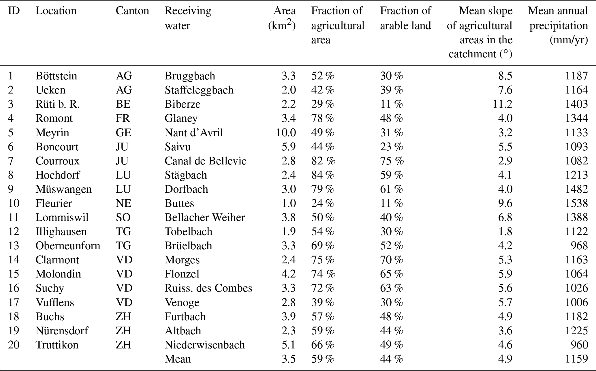
Figure 1 Study areas (black) and distribution of arable land (brown), vineyards (pink), and meadows and/or pastures (green) across Switzerland. Sources: Swisstopo (2010); BFS (2014).

2.2 Assessment of hydraulic shortcuts

2.2.1 Shortcut definition

We define a hydraulic shortcut as an artificial structure increasing and/or accelerating the process of surface runoff reaching surface waters (i.e. rivers, streams, and lakes) or making this process possible in the first place. In this study, we focused on the following structures (example photographs can be found in Figs. S2 to S13):

• a.

  storm drainage inlet shafts on roads, farm tracks, and crop areas;

• b.

  maintenance shafts of storm drainage systems or tile drainage system on roads, farm tracks, and crop areas; and

• c.

  channel drains and ditches on roads, farm tracks, and crop areas.

If one of these structures is present, we defined this as a potential shortcut. If surface runoff can enter the structure and if the structure is drained to surface waters or to a wastewater treatment plant, this is defined as a real shortcut. Other processes that are sometimes referred to as hydraulic shortcuts (e.g. tile drains) are not considered in this study. Tile drains have already received considerable attention in pesticide research and the transport to tile drains includes flow through natural soil.

2.2.2 Shortcut location and type

We mapped the location and types of potential shortcuts in each study area by combining three different methods.

• i.

  Field survey. Field surveys were performed between August 2017 and May 2018 (for details, see Table S5). In a subpart of each study area, we walked along roads and paths and mapped all the potential shortcut structures. The starting point was selected randomly, and we mapped as much as we could within 1 d. Consequently, the field survey data only cover part of the catchment. For each of the potential shortcuts, we recorded its location and a set of properties using a smartphone and the application called Google My Maps. This included a specification of the type of the shortcut (e.g. inlet shaft, maintenance shaft, ditch, or channel drain), its lid type (e.g. grid, sealed lid, or a lid with small openings), and its lid height relative to the ground surface. A list of all possible types can be found in the Supplement (Tables S2 to S4).

• ii.

  Drainage plans. For all municipalities covering more than 5 % of a study area, we asked the responsible authorities to provide us with their plans of the road storm drainage systems and the agricultural drainage systems. For 38 and 26 of the 46 municipalities concerned, we received road storm drainage system plans and tile drainage system plans, respectively. Reasons for missing data are either that the responsible authorities did not respond or that data on the drainage systems were not available. From the plans, we extracted the locations of shortcuts, and if available, the same properties were specified as in the field survey.

• iii.

  Aerial images. Between August 2017 and August 2018 (see Table S5), we acquired aerial images of the study areas with a ground resolution of 2.5 to 5 cm. We used a fixed wing UAV (unoccupied aerial vehicle; eBee, senseFly, Cheseaux-sur-Lausanne) in combination with a visible light camera (Sony DSC-WX220; RGB). The study areas were fully covered by the UAV imagery, with the exception of larger settlement areas, forests, lakes, and no-fly zones for drones (e.g. airports). The UAV images were processed to one georeferenced aerial image per study area using the software Pix4Dmapper 4.2. In the no-fly zones of the study areas in Meyrin (Geneva), Buchs (Zürich), and Nürensdorf (Zürich), we used aerial images provided by the cantons of Geneva (Etat de Genève, 2016) and Zürich (Kanton Zürich, 2015). Ground resolutions were 5 and 10 cm respectively. Using ArcGIS 10.7, we gridded the aerial images, scanned by eye through each of the grid cells, and marked all potential shortcut structures manually. If observable from the aerial image, the same properties as for the field survey were specified for each potential shortcut structure.

  We combined the three data sets originating from the three methods to a single data set. If a potential shortcut structure was only found by one of the mapping methods, its location and type were used for the combined data set. If it was found by more than one of the mapping methods, we used the location and type of the mapping method that we expected to be the most accurate. For the location information and the type specification, we used UAV imagery, before field survey, and maps.

2.2.3 Assigning shortcuts to landscape elements

In order to better understand where hydraulic shortcuts occur the most, we assigned them to different landscape elements. Using the topographic landscape model of Switzerland, swissTLM3D (Swisstopo, 2010), we defined five landscape elements, namely paved roads, unpaved roads, fields, settlements, and other areas (e.g. railways, other traffic areas, forests, water bodies, wetlands, and single buildings). For all landscape elements except roads and railways, shortcuts were assigned to their landscape elements by a simple intersection. However, shortcuts belonging to road or railway drainage systems are, in many cases, not placed directly on the road or railway but on the adjacent agricultural land or settlement. Therefore, shortcuts were assigned to the landscape elements of road or railway if they were within a 5 m buffer.

In addition, we correlated the density of shortcuts per study area to different study area properties. We selected properties that we expected to have explanatory power, i.e. density (length per area) of paved roads, density of unpaved roads, density of surface rivers, density of subsurface rivers, mean annual precipitation, and mean slope on agricultural areas.

2.2.4 Drainage of shortcuts

A potential shortcut only turns into a real one if it is drained to surface waters by pipes or other connecting structures such as ditches. Therefore, using the plans provided by the municipalities, we investigated where potential shortcuts drain to. They were allocated to one of the following categories of recipient areas, namely surface waters, wastewater treatment plants and/or combined sewer overflows, infiltration areas (e.g. forests, infiltration ponds, fields, and grassland), or unknown.

2.3 Surface runoff connectivity model

To assess how hydraulic shortcuts contribute to surface runoff connectivity, we created a surface runoff connectivity model.

The model is based on the concept of critical source areas (CSAs; see introduction). It mainly focuses on the first two elements of the CSA concept (i.e. pesticide application and connectivity to surface waters). In contrast, the question of whether an area is hydrologically active is only addressed partially because much relevant information, such as soil properties, is not available at the national scale.

The model (see Fig. 2) distinguishes source areas on which surface runoff is produced, and recipient areas on which surface runoff ends up. A connectivity model connects those areas by routing surface runoff through the landscape. These model parts are conceptually described in more detail in Sect. 2.3.1. In Sect. 2.3.2, we describe how we parameterized the model, and how we assessed the uncertainty of model output given the parameter uncertainty. In Sect. 2.3.3, we explain the testing for systematic differences in the hydrological activity between areas with direct or indirect connectivity.

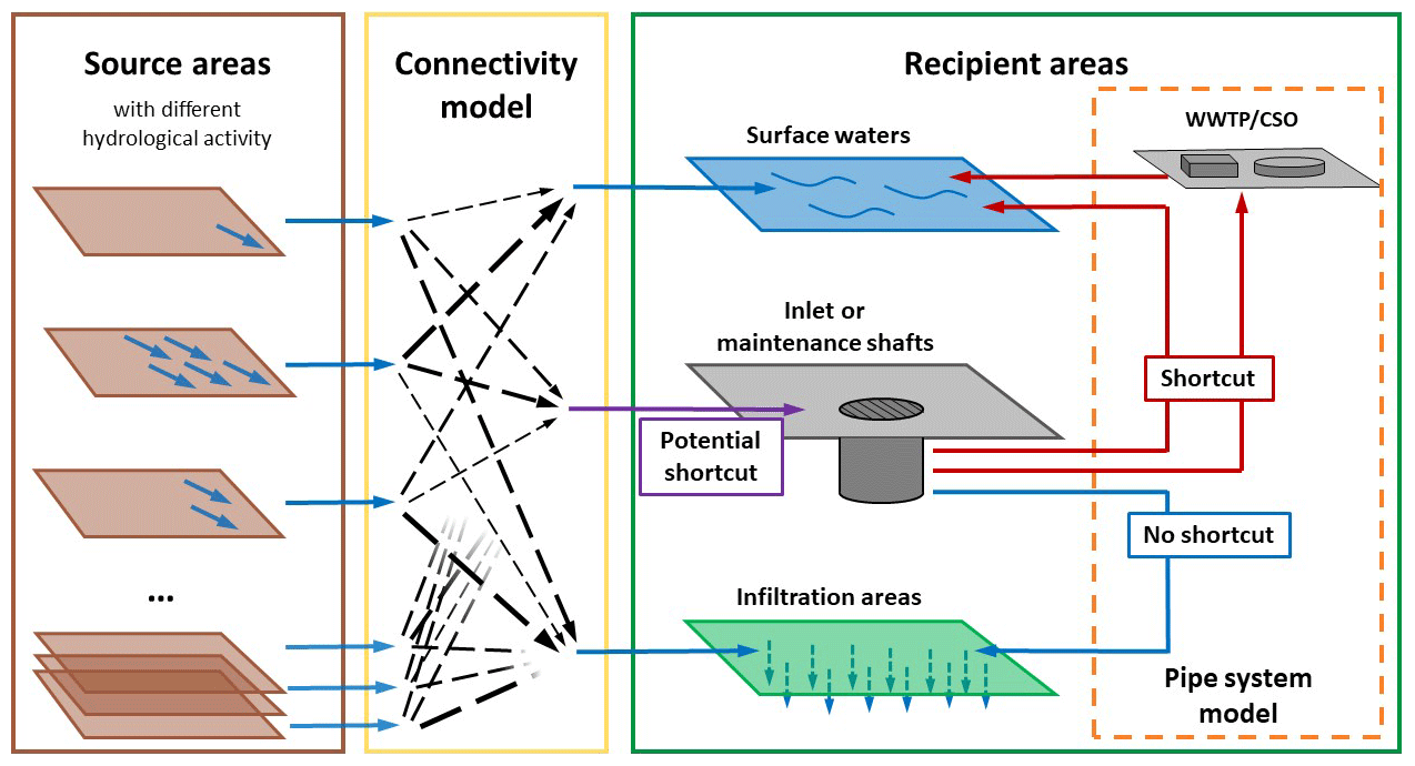
Figure 2 Structure of the surface runoff connectivity model. WWTPs – wastewater treatment plants; CSO – combined sewer overflow.

2.3.1 Model structure

Source areas. All crop areas on which pesticides are applied should, in theory, be considered as source areas. However, a highly resolved spatial data set of land in a crop rotation for our study areas is lacking. Therefore, we considered the total extent of agricultural areas (i.e. arable land, meadows and/or pastures, vineyards, orchards, and gardening) as source areas, since those areas could be derived in high resolution. The extent of agricultural areas was defined by subtracting all non-agricultural areas from the extent of the study area. For this, we used non-agricultural areas (forests, water bodies, urban areas, traffic areas, and other non-agricultural areas) as defined by the national topographical landscape model swissTLM3D (Swisstopo, 2010). According to the Swiss proof of ecological performance (PEP), pesticide usage within a distance of 6 m from a river and within 3 m from hedges and forests is prohibited. The extent of agricultural areas was reduced accordingly, except along forests (parameters – river spray buffer and hedge spray buffer).

Recipient areas. Surface runoff generated on a source area and routed through the landscape can end up in three different types of landscape elements, referred to as recipient areas, namely surface waters, infiltration areas (i.e. forests, hedges, and internal sinks), and shortcuts. The extent of surface waters (rivers that have their course above the surface, lakes, and wetlands), was defined by the swissTLM3D model, as was the extent of forests and hedges. Since forests and hedges are known to infiltrate surface runoff (Sweeney and Newbold, 2014; Schultz et al., 2004; Bunzel et al., 2014; Dosskey et al., 2005), we assumed that forests with a certain width (parameter–infiltration width) act as an infiltration area. Hedges were assumed to either act as infiltration areas or to have no effect on surface runoff. Accordingly, the parameter hedge infiltration was varied between yes (hedges act as infiltration areas) and no (hedges do not act as an infiltration areas).

Internal sinks in the landscape were defined using the 2×2 m digital elevation model (DEM; Swisstopo, 2018). All sinks larger than two raster cells and deeper than a certain depth (parameter–sink depth) were defined as internal sinks. All other sinks were filled completely.

Shortcuts were defined in two different ways (parameter – shortcut definition). In definition A, all inlet shafts, ditches, and channel drains were considered as potential shortcuts. In definition B, maintenance shafts lying in internal sinks were additionally considered as potential shortcuts. Potential shortcuts were defined to act as real shortcuts if they are known to discharge to surface waters or wastewater treatment plants. From the drainage plans of the municipalities, we know that most of the inlet shafts discharge into either a surface water body or a wastewater treatment plant. Therefore, also potential shortcuts with unknown drainage location were assumed to act as real shortcuts. Potential shortcuts discharging into forests or infiltration structures were assumed not to act as shortcuts and were not used in the model. Shortcut recipient areas were defined as the raster cells of the digital elevation model on which the shortcut is located and all the cells directly surrounding it (see Fig. S14 in the Supplement).

Connectivity model. For modelling connectivity, we used the TauDEM model (Tarboton, 1997), which is based on a D-infinity flow direction approach. As an input, we used a 2×2 m digital elevation model (Swisstopo, 2018). This DEM was modified as follows. We assumed that only those internal sinks that were defined as sink recipient areas (see above) effectively act as sinks. Therefore, first, all sinks were filled, and sink recipient areas were carved 10 m into the DEM. Second, all other recipient areas (shortcuts, forests, hedges, and surface waters) were carved between 10 and 50 m into the DEM. Carving the recipient areas into the DEM ensured that surface runoff reaching a recipient area was not routed further on to another recipient area. Third, to account for the effect of roads accumulating surface runoff (Heathwaite et al., 2005), roads were carved into the DEM by a given depth defined by the parameter road carving depth.

The modified DEM, the source areas, and the recipient areas were used as an input into the TauDEM tool of D-infinity upslope dependence. In this way, each raster cell belonging to a source area was assigned with the probability of being drained into one of the three types of recipient areas.

The connectivity of a source area may depend on the flow distance to surface waters. For longer flow distances, water has a higher probability of infiltrating before it reaches a surface water. Therefore, for each source area raster cell, we calculated the flow distance to its recipient area using the tool D-infinity distance down.

2.3.2 Model parametrization and sensitivity analyses

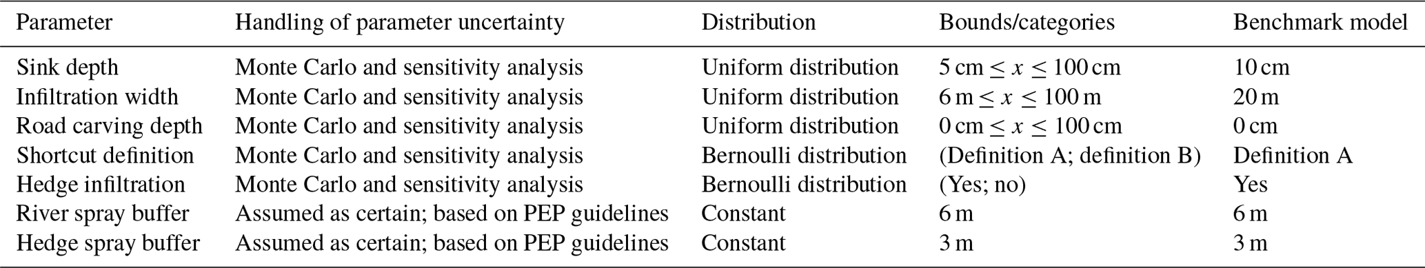
The model parameters mentioned in the section above vary in space and time. Since this variability could not be addressed with the selection of a single parameter value, we performed a Monte Carlo simulation with 100 realizations. The probability distributions of the parameters are provided in Table 2. The bounds or categories of these distributions were based on our prior knowledge about the hydrological processes involved, about structural aspects (e.g. depths of sinks), and on our experience from field mapping. The parameters river spray buffer and hedge spray buffer were assumed constant according to the guidelines of the Swiss proof of ecological performance (PEP).

To assess the influence of single parameters on our modelling results, we performed a local sensitivity analysis against a benchmark model (one realization of the model with a specific parameter set; see Table 2). When selecting the benchmark model parameter set, we kept the changes in the digital elevation model small (i.e. road carving depth is 0 cm; sink depth is 10 cm). For the other model parameters, we selected the values that we assumed to be the most probable in reality. For the local sensitivity analysis, each of the model parameters was varied individually within the same boundaries as for the Monte Carlo analysis.

Table 2 Summary of parameter distributions used for the Monte Carlo analysis and parameter values used as a benchmark for the sensitivity analysis. PEP – Swiss proof of ecological performance.

2.3.3 Hydrological activity

As mentioned earlier, a critical source area has to be hydrologically active, i.e. surface runoff has to be generated on that area. Runoff generation depends on many variables (e.g. crop types, soil types, soil moisture, and rain intensity) for which no data are available in most of our study areas and which are strongly variable over time. Since we are interested in the general relevance of shortcuts, we focused on the question of whether there is a systematic difference in the hydrological activity between areas directly or indirectly connected to streams.

For soil moisture, we tested for such differences by calculating the distribution of the topographic wetness index (TWI; Beven and Kirkby, 1979) for the source areas of the benchmark model. We calculated the TWI as follows, using the tool in the TauDEM model:

$$\begin{array}{}\text{(1)}& \mathrm{TWI}={\displaystyle \frac{\ln \left(a\right)}{\tan \left(\mathit{\beta }\right)}}.\end{array}$$

The local upslope area a and the local slope β were calculated using the D-infinity flow direction algorithm that was already used for the surface runoff connectivity model. As an input, we used the source areas and the modified DEM as specified for the surface runoff connectivity model.

The formation of surface runoff on agricultural areas is also influenced by their slope. Therefore, we calculated the distribution of slopes for source areas draining to different destinations. For this, we used the slopes from the Swiss digital elevation model (Swisstopo, 2018).

For other variables (e.g. crop type and rain intensity), there is no indication of such systematic differences. Therefore, we assumed that they do not differ systematically between areas draining to different recipient areas.

2.4 Extrapolation to the national level

2.4.1 Extrapolation of the local connectivity model

In a last step, we developed a model to extrapolate the results from our study areas (local surface runoff connectivity model – LSCM) to the national scale. This extrapolation was then used to evaluate how the results of this study compare to a pre-existing connectivity model (national erosion connectivity model – NECM; Alder et al., 2015).

Selection of explanatory variables. We calculated a list of catchment statistics based on nationally available geo-data sets that could serve as explanatory variables. As catchment boundaries, the polygons from the national catchment data set (BAFU, 2012) were used. Details on the data sets used for calculating those catchment statistics can be found in Table S1.

We created a linear regression between each of those catchment statistics to the median fractions of agricultural areas directly, indirectly, and not connected to surface waters, as reported by the LSCM (f_LSCM,dir, f_LSCM,indir, f_LSCM,nc). The strongest correlations were found for the fractions of agricultural areas directly, indirectly, and not connected to surface waters, as reported by the NECM (f_NECM,dir, f_NECM,indir, and f_NECM,nc; see Table S8). Therefore, we used them as explanatory variables to build an extrapolation model of our local results to the national scale.

The model predictions for each catchment have to fulfil specific boundary conditions. First, the sum of areal fractions of the three types of recipient areas k per catchment c has to equal one (${\sum }_{k=\mathrm{1}}^K{f}_{k,c}=\mathrm{1}$), and second, area fractions cannot be negative ($f_{k,c}\ge \mathrm{0}$). To ensure these conditions, we performed the model fit after a unit simplex data transformation. To address the uncertainty introduced by the selection of our study catchments, we additionally bootstrapped the model 100 times. The resulting modelling approach is shown in Fig. 3. Mathematical details are provided in the Supplement (Sect. S1.5).

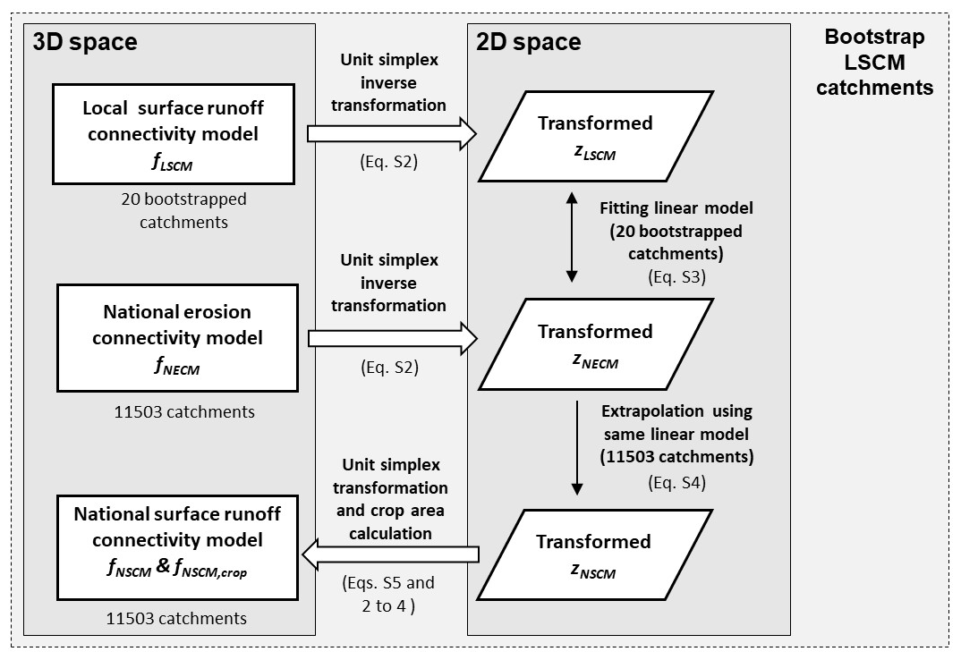
Figure 3 Extrapolation of the local surface runoff connectivity model (LSCM) to the national scale (NSCM) using a unit simplex transformation approach. Equations (2)–(4) are shown in Sect. 2.4.2. Equations (S2)–(S5) are provided in the supplement (Sect. S1.5).

As a result, we obtained a national surface runoff connectivity model (NSCM). The NSCM provides an estimate for the fractions of agricultural areas directly, indirectly, and not connected to surface waters (f_NSCM,dir, f_NSCM,indir, and f_NSCM,nc) for the catchments of the national catchment data set. Since mountainous regions of higher altitudes are excluded in the NECM, those areas are also excluded in the NSCM.

2.4.2 Connectivity of crop areas

During the time of this study, high-resolution data sets of Swiss crop areas were not available in Switzerland. Therefore, we considered the total extent of agricultural areas for building the local surface runoff connectivity model and extrapolation to the national scale. This includes areas with rare pesticide application, such as meadows and pastures.

The Swiss land use statistics data set (BFS, 2014) is a raster data set with a resolution of 100 m, dividing agricultural areas into different categories (e.g. arable land, vineyards, and meadows and/or pastures). On the national scale, the use of such a lower-resolution data set is more reasonable. Hence, we used this data set to calculate fractions of connected crop areas.

The fractions of directly, indirectly, and not connected crop areas per total agricultural area per catchment c ($f_{\mathrm{NSCM},\mathrm{crop},c}$) were calculated as follows:

$$\begin{array}{}\text{(2)}& f_{\mathrm{NSCM},\mathrm{crop},c}=f_{\mathrm{NSCM},c}\cdot r_{\mathrm{crop},c},\end{array}$$

with r_crop being the ratio of crop area to total agricultural area in a catchment, as follows:

$$\begin{array}{}\text{(3)}& {\displaystyle }& {\displaystyle }{r}_{\mathrm{crop},c}={\displaystyle \frac{A_{\mathrm{crop},c}}{A_{\mathrm{crop},c}+A_{\mathrm{mead},c}}}\text{(4)}& {\displaystyle }& {\displaystyle }{A}_{\mathrm{crop},c}=A_{\mathrm{arab},c}+A_{\mathrm{vin},c}+A_{\mathrm{orch},c}+A_{\mathrm{gard},c},\end{array}$$

where, in catchment c, A_crop,c is the crop area, A_mead,c is the meadow and pasture area, A_arab,c is the arable land area, A_vin,c is the vineyard area, A_orch,c is the orchard area, and A_gard,c is the gardening area.

3 Results

3.1 Occurrence of hydraulic shortcuts

In the following section, we first show the results of the field mapping campaign for shafts (inlet and maintenance shafts), followed by the results for channel drains and ditches. Afterwards, we present results on the accuracy of our mapping methods.

3.1.1 Shafts

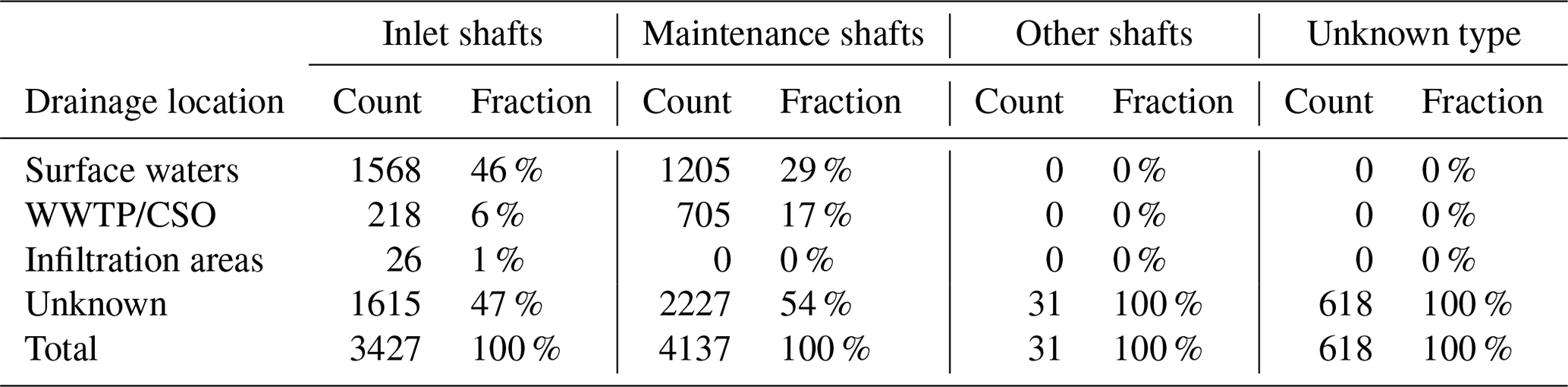
In total, we found 8213 shafts, corresponding to an average shaft density of 2.0 ha⁻¹ (min – 0.51 ha⁻¹; max – 4.4 ha⁻¹; Table 3). A total of 42 % of the shafts mapped were inlet shafts. A plot showing the density of shafts mapped per catchment and shaft type can be found in Fig. S15.

For roughly half of the inlet and maintenance shafts, we were able to identify a drainage location. Both shaft types discharge in almost all cases into surface waters, either directly (87 % of inlet shafts; 63 % of maintenance shafts) or via wastewater treatment plants or combined sewer overflows (12 % of inlet shafts; 37 % of maintenance shafts). Only 1.4 % of the inlet shafts and no maintenance shaft at all, were found to drain to an infiltration area such as forests or fields.

Table 3 Number of shafts found in agricultural areas of the study areas per shortcut category and drainage location. WWTP – wastewater treatment plant; CSO – combined sewer overflow.

Most of the inlet shafts mapped (90 %) are located on paved or unpaved roads (see Table 4). Only very few inlet shafts (2.8 %) are found directly on fields. In contrast, maintenance shafts are found much more often on fields and, therefore, less often on paved or unpaved roads. The fractions of inlet and maintenance shafts belonging to a certain landscape element for each study area can be found in Figs. S17 and S18.

Table 4 Percentage of shafts found in a certain type of landscape element. The category of other areas integrates several types of landscape elements, including railways, other traffic areas, forests, water bodies, wetlands, and single buildings.

We correlated the densities of inlet and maintenance shafts per study area with possible explanatory variables. Only the density of paved roads was significantly correlated to the density of inlet shafts (R²= 0.33; p= 0.008) and maintenance shafts (R²=0.37; p= 0.005; see Tables S6 and S7).

3.1.2 Channel drains and ditches

In addition to shafts, we also mapped channel drains and ditches. With the exception of the study areas Meyrin (4.2 m ha⁻¹) and Buchs (4.0 m ha⁻¹), these structures were rarely found (< 1.2 m ha⁻¹; see Fig. S16). In Meyrin and Buchs, most channel drains and ditches (98 % of the total length) drain to surface waters, and only few of them to infiltration areas (2 %).

3.1.3 Mapping accuracy

The results above were generated using three different mapping methods (field survey, aerial images, and drainage plans). These methods differ in their ability to identify and classify a potential shortcut structure correctly and in the study area they cover. We determined the accuracy of the mapping methods for aerial images and drainage plans using the field survey method as a ground truth (see Table 5) for those parts of the study areas where all three methods were applied. Since channel drains and ditches were rare, this assessment was only performed for shafts.

The recall (i.e. the probability that a potential shortcut is found by a mapping method) was limited for the aerial images method (53 % for inlet shafts; 62 % for maintenance shafts) and even lower for the drainage plans method (32 % for inlet shafts; 21 % for maintenance shafts). However, identified shortcuts were, in most of the cases, classified correctly (accuracy – 93 % to 94 % for aerial images; 88 % to 89 % for drainage plans).

For the entire study area, Fig. 4 shows the number of potential shortcuts identified by the three mapping methods. Despite a low recall, aerial images identified the largest number of potential shortcuts. This is due to the large spatial coverage by the aerial images method. Since the overlap between the three methods is small (only 32 % of the inlet shafts and 15 % of the maintenance shafts were found by more than one method), each of the methods was important for determining the total number of potential shortcuts in the study areas. Because the aerial images and drainage plans have a low recall but cover large parts of the study areas that were not assessed by the field survey, the numbers reported above are a lower boundary estimate.

Table 5 Recall and classification accuracies of the mapping methods of aerial images and drainage plans. The recall corresponds to the probability that a potential shortcut is found by the mapping method. Percentages indicate the recall of each individual mapping method. In parentheses, the recall of the combination of both methods is given. The accuracy corresponds to the sum of true positive fraction and true negative fraction.

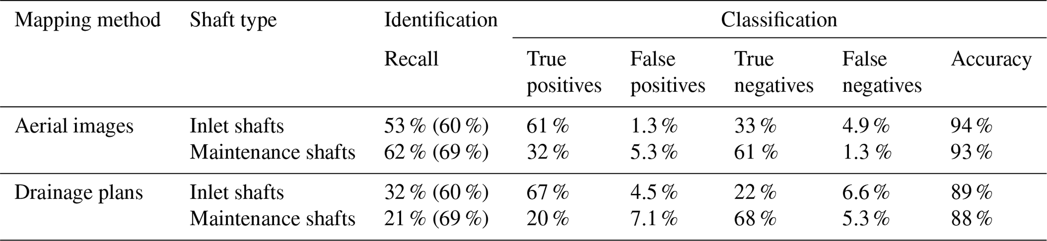
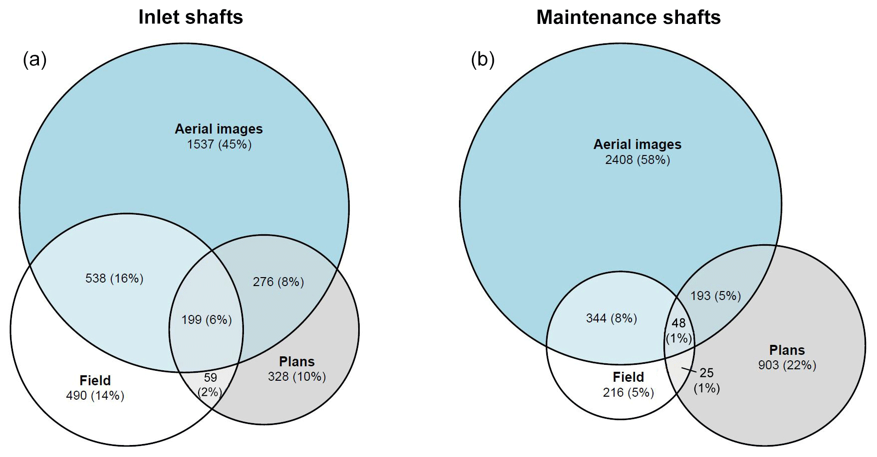
Figure 4 Number of inlet (a) and maintenance shafts (b) identified by the different mapping methods.

3.2 Surface runoff connectivity

3.2.1 Study areas

From the Monte Carlo analysis of the surface runoff connectivity model, we obtained an estimate for the fractions of agricultural areas that are connected directly, indirectly, or not at all to surface waters. To illustrate the variability resulting from these Monte Carlo (MC) runs, Fig. 5 shows the output of three MC simulations (MC28, MC41, and MC40) for Molondin. These simulations correspond to the 5 %, 50 %, and 95 % quantile of the median fraction of indirectly connected per total connected agricultural area over all study catchments. The classification of certain catchment parts is changing, depending on the model parameterization (e.g. letters A to C). However, for other parts, the results are consistent across the different MC simulations (e.g. letters D to F). Overall, the results show that not only agricultural areas close to surface waters (e.g. letter D) are connected to surface waters. Hydraulic shortcuts also create surface runoff connectivity for areas far away from surface waters (e.g. letter E).

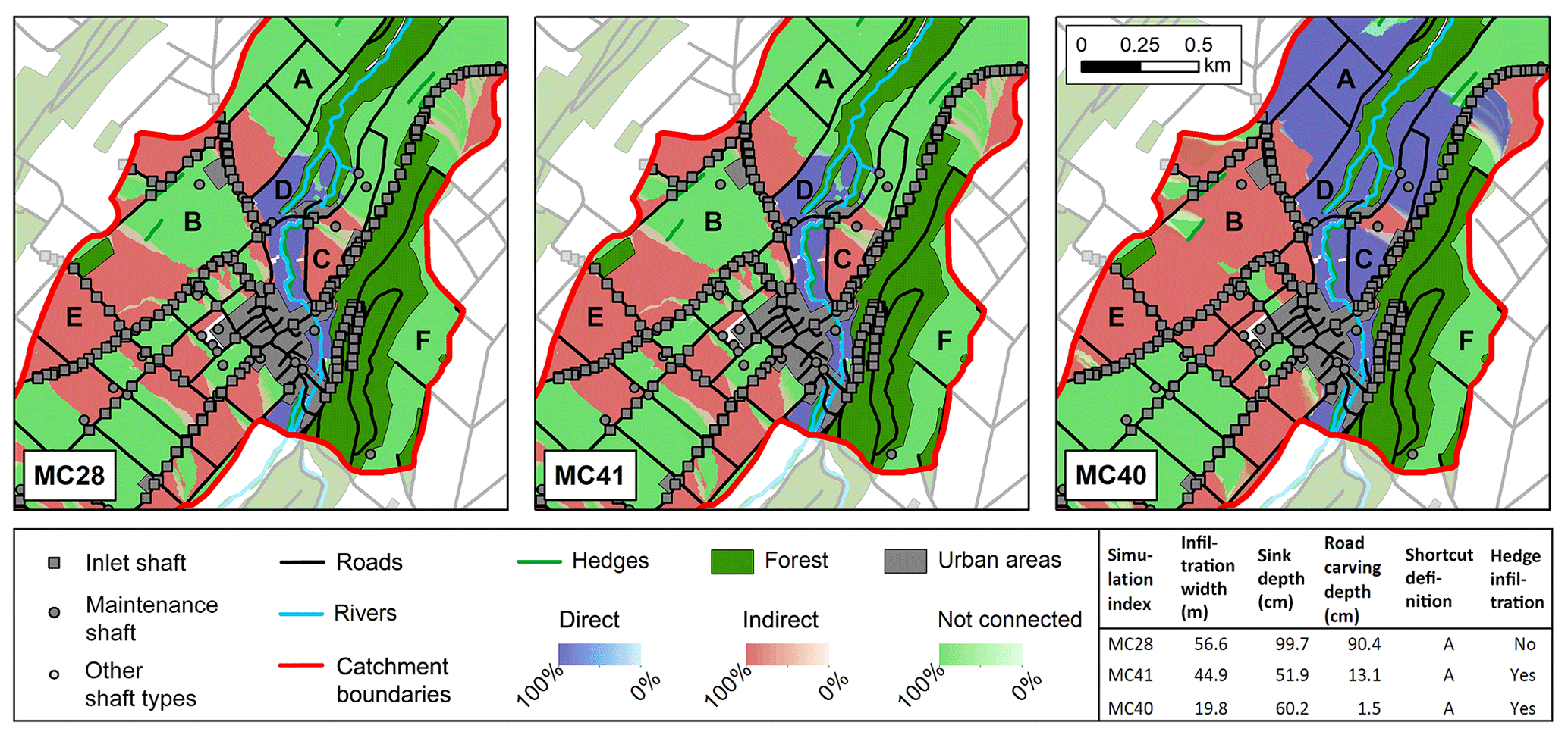
Figure 5 Results of three example Monte Carlo (MC) simulations for a part of one study area (Molondin). The colour ramps show the probability of agricultural areas to be directly connected (blue), indirectly connected (red), and not connected (green). The simulations represent, approximately, the 5 % (MC28), 50 % (MC41), and 95 % (MC40) quantiles with respect to the resulting median fractions of indirectly connected per total connected area over all study catchments. The parameters of the example MC simulations are shown at the bottom right. Source of background map: Swisstopo (2010).

In order to assess the importance of hydraulic shortcuts, we calculated the fraction of the indirectly connected area to the total connected area. Across all Monte Carlo simulations, the median of this fraction over all study catchments ranges between 43 % and 74 % (mean – 57 %; median – 58 %; Fig. 6). Despite considerable uncertainty, the results demonstrate that a large fraction of the surface runoff connectivity to surface waters is established by hydraulic shortcuts.

Figure 6 (a) Fractions of indirectly connected areas per total connected areas as calculated by the Monte Carlo analysis for each study area. White dots indicate the means of the distributions. The red dots indicate the results of the example Monte Carlo simulations (MC28, MC41, and MC 40) shown in Fig. 5. (b) Distribution of medians of fractions of indirectly connected areas per total connected areas per study catchment and per Monte Carlo simulation.

For different flow distances, the fraction of indirectly connected area to the total connected area underlies only minor variations (see Fig. S24). However, this fraction varies strongly between the study areas, with median fractions ranging from 21 % in Müswangen to 97 % in Boncourt. Although the occurrence of hydraulic shortcuts is a prerequisite for indirect connectivity, high shaft densities are not necessarily leading to high fractions of indirect connectivity in a catchment. The densities of inlet and maintenance shafts show only a weak positive correlation to the catchment medians of the fraction of indirectly connected areas (inlet shafts – R²= 0.11 and p= 0.15; maintenance shafts – R²= 0.08 and p= 0.23; see Table S8). By contrast, the two study areas with high channel drain and ditch densities (Meyrin and Buchs) show high fractions of indirect connectivity. Similarly, the density of surface waters is strongly negatively correlated to the fraction of indirect connectivity (R²= 0.51; p < 0.001). This suggests that line elements like channel drains, ditches, and surface waters usually have an influence on connectivity if they occur in a catchment. In contrast, the influence of point elements seems to depend a lot on the surrounding landscape structure.

As a further consequence of the structural differences between the study areas, not all of them reacted the same way to changes in model parameters of the Monte Carlo analysis. For example, the fraction of indirectly to total connected areas in the study area Boncourt was quite insensitive to changes in model parameters. Since Boncourt has a very low water body density, only small areas are connected directly, which is independent of the model parameterization. The study area Illighausen, on the other hand, reacted very sensitively (range of results – 68 %). Since Illighausen is a very flat catchment, changes in the sink depth parameter had a large influence on the estimated fractions of direct and indirect connectivity.

So far, we only reported on the fraction of indirectly connected per total connected area. In Table 6, we additionally report the fractions of total agricultural area connected directly, indirectly, and not at all to surface waters. On average, we estimate between 5.5 % and 38 % (mean – 28 %) of the agricultural area to be connected directly, 13 % to 51 % (mean – 35 %) to be connected indirectly, and 12 % to 77 % (mean – 37 %) not to be connected to surface waters. However, the variation between the catchments is much larger than the variation of the Monte Carlo analysis.

Table 6 Fractions of directly, indirectly, and not connected agricultural areas in our study catchments. The first row represents the mean fraction over all catchments and Monte Carlo simulations. The second row represents the median of the median over all catchments per MC simulation. The third row represents the median of the median over all MC analyses per catchment. In parentheses, the minimum and the maximum median are given.

3.2.2 Sensitivity analysis

To analyse which model parameters have the largest influence on our model results, we tested the local model parameter sensitivity on our benchmark model. The fraction of indirectly to total connected area has the most sensitive reaction to changes in the road carving depth parameter. The difference between the minimal and maximal fraction reported was 17 %. Results were also sensitive to the parameters shortcut definition (14 %) and sink depth (13 %). Infiltration width (4.3 %) and hedge infiltration (2.5 %) had only a minor influence on the fraction reported (see Figs. S22 and S23).

3.2.3 Hydrological activity

Systematic differences in hydrological activity between directly and indirectly connected areas would have a major influence on the interpretation of our connectivity analysis. We, therefore, tested for such differences by calculating the distributions of slope and topographic wetness index on these areas.

The distributions of both slope and topographic wetness index were very similar for directly, indirectly, and not connected areas (see Figs. S25 and S26). Only the slope of not connected areas was found to be slightly smaller than the slope of connected areas. Hence, we could not identify any systematic differences in the factors affecting hydrological activity between directly and indirectly connected areas.

Consequently, given the current knowledge, the proportions of direct and indirect surface runoff entering surface waters are expected to be equal to the proportions of directly and indirectly connected agricultural areas. Analogously, if other boundary conditions of pesticide transport remain unchanged, directly and indirectly transported pesticide loads are expected to be proportional to directly and indirectly connected crop areas.

3.2.4 Extrapolation to the national level

We created a model for extrapolating the results of our study areas to the national level, using area fractions of the national erosion connectivity model (NECM; Alder et al., 2015) aggregated to the catchment scale as explanatory variables. The area fractions of the NECM were transformed such that they fit the area fractions of the local surface runoff connectivity model (LSCM) resulting from the Monte Carlo analysis in our study areas. The resulting data set is called the national surface runoff connectivity model (NSCM). The NSCM provides a separate model for each of the 100 Monte Carlo runs of the LSCM. It is aggregated to the catchment scale and covers all catchments of the valley zones, hill zones, and lower elevation mountain zones. The differences between the fitted NSCM and the LSCM were strongly reduced compared to the original NECM (see Fig. 7). The root mean square error (RMSE), on average, reduced from 17 % to 9.5 % for directly connected fractions, from 12 % to 7.6 % for indirectly connected fractions, and from 18 % to 7.6 % for not connected fractions.

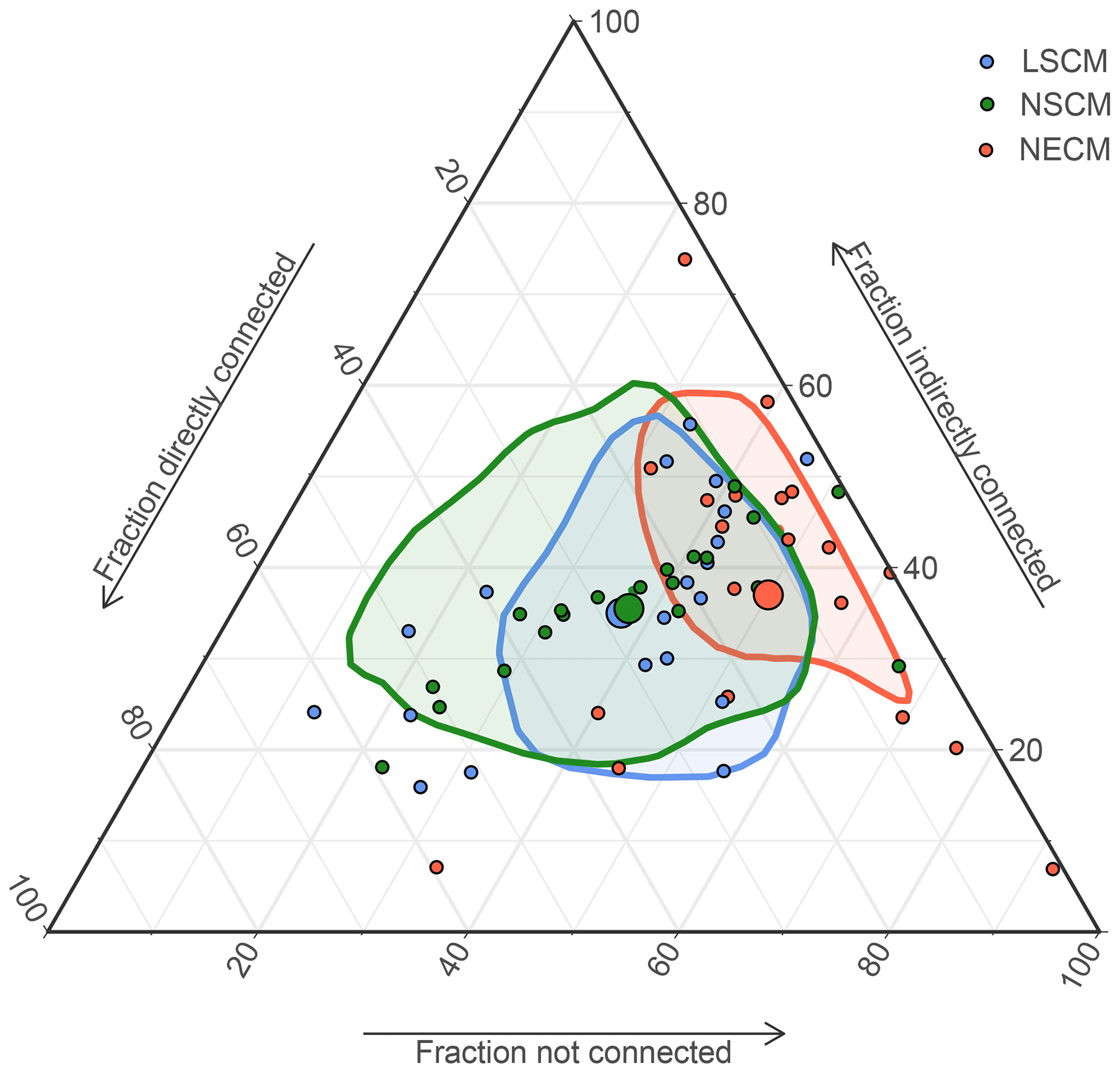
Figure 7 Fractions (%) of directly connected (f_dir), indirectly connected (f_indir), and not connected areas (f_nc) per total agricultural area for the local surface runoff connectivity model (LSCM; blue), national erosion connectivity model (NECM; red), and national surface runoff connectivity model (NSCM; green) in the 20 study areas. Small blue circles represent the catchment medians of all Monte Carlo simulations of the LSCM, small red circles represent the data reported by the NECM, and small green circles represent the catchment medians of the NSCM. Large circles represent the means of the LSCM (blue), NECM (red), and NSCM data (green). Shaded areas represent normal kernel density estimates of the LSCM, NECM, and NSCM data.

By combining the NSCM with land use data, we came up with an estimate of connected crop areas on the national scale. Half of the Swiss agricultural areas in the model region are crop areas (i.e. arable land, vineyards, orchards, and horticulture) and, therefore, potential pesticide source areas. On average, 26 % of crop areas (13 % of total agricultural area) are connected directly, 34 % (17 % of total agricultural area) indirectly, and 40 % (20 % of total agricultural area) not at all (see Fig. S27 for details; for MC simulation quantiles, see Table S9; for spatial distribution, see Figs. S30 to S36). From the total connected crop area, 54 % (between 47 % and 60 %) are connected indirectly.

These results are similar to those obtained for the 20 study areas. Mean fractions of directly and indirectly connected agricultural areas are a bit smaller in the national scale estimation than for the 20 study areas (−2.0 % and −1.9 %), while the fraction of not connected agricultural area is a bit larger (+3 %). The fraction of indirectly connected crop area per total connected crop area is slightly smaller (−2.6 %).

To assess if the national erosion connectivity model (NECM) is different from the national surface runoff connectivity model (NSCM), we determined the 5 % and 95 % quantiles of the NSCM predictions (see Table S9). If a fraction of the NECM is outside of this range, we considered this as a significantly different model prediction that is not expected given our field data.

Compared to the NSCM, the NECM, on average, predicts lower fractions of directly connected crop areas f_crop,dir (−6.4 %), which is below the 5 % quantile of the NSCM results. For indirectly connected areas f_crop,indir (−0.9 %) and not connected crop areas f_crop,nc (+7.2 %), the data reported by the NECM are within the 5 % and 95 % quantile of the NSCM results. However, the fraction of indirectly connected crop area per total connected crop area f_fracindir reported by the NECM lies beyond the 95 % quantile of the NSCM (+11 %). In summary, f_crop,dir and f_fracindir reported by the NECM are significantly different from what would be expected from the NSCM. For f_crop,indir and f_crop,nc, the reported fractions are in a similar range for both models. The results of the bootstrap (Fig. S28) show that the differences between the two models are significantly larger than the uncertainty introduced by the selection of the study catchments.

The average difference in predicted connectivity fractions of agricultural areas between the two models ($\mathrm{\Delta }f=\left(\right(f_{\mathrm{NSCM},\mathrm{dir}}-f_{\mathrm{NECM},\mathrm{dir}})+(f_{\mathrm{NSCM},\mathrm{indir}}-f_{\mathrm{NECM},\mathrm{indir}})$ $+(f_{\mathrm{NSCM},\mathrm{nc}}-f_{\mathrm{NECM},\mathrm{nc}}))/\mathrm{3}$) is strongly variable in space. Large differences are mainly found in large valleys (e.g. the Aare, Alpenrhein, and Rhône valleys and the valleys of Ticino) and in the region of Lake Constance (see Fig. S40). However, when looking at the difference in average predicted connectivity fractions of crop areas ($\mathrm{\Delta }{f}_{\mathrm{crop}}=\left(\right(f_{\mathrm{NSCM},\mathrm{crop},\mathrm{dir}}-f_{\mathrm{NECM},\mathrm{crop},\mathrm{dir}})+(f_{\mathrm{NSCM},\mathrm{crop},\mathrm{indir}}-f_{\mathrm{NECM},\mathrm{crop},\mathrm{indir}})+(f_{\mathrm{NSCM},\mathrm{crop},\mathrm{nc}}-f_{\mathrm{NECM},\mathrm{crop},\mathrm{nc}}\left)\right)/\mathrm{3}$), large differences are almost exclusively found in a band of catchments with high crop densities spreading through the Swiss midlands (see Fig. 8).

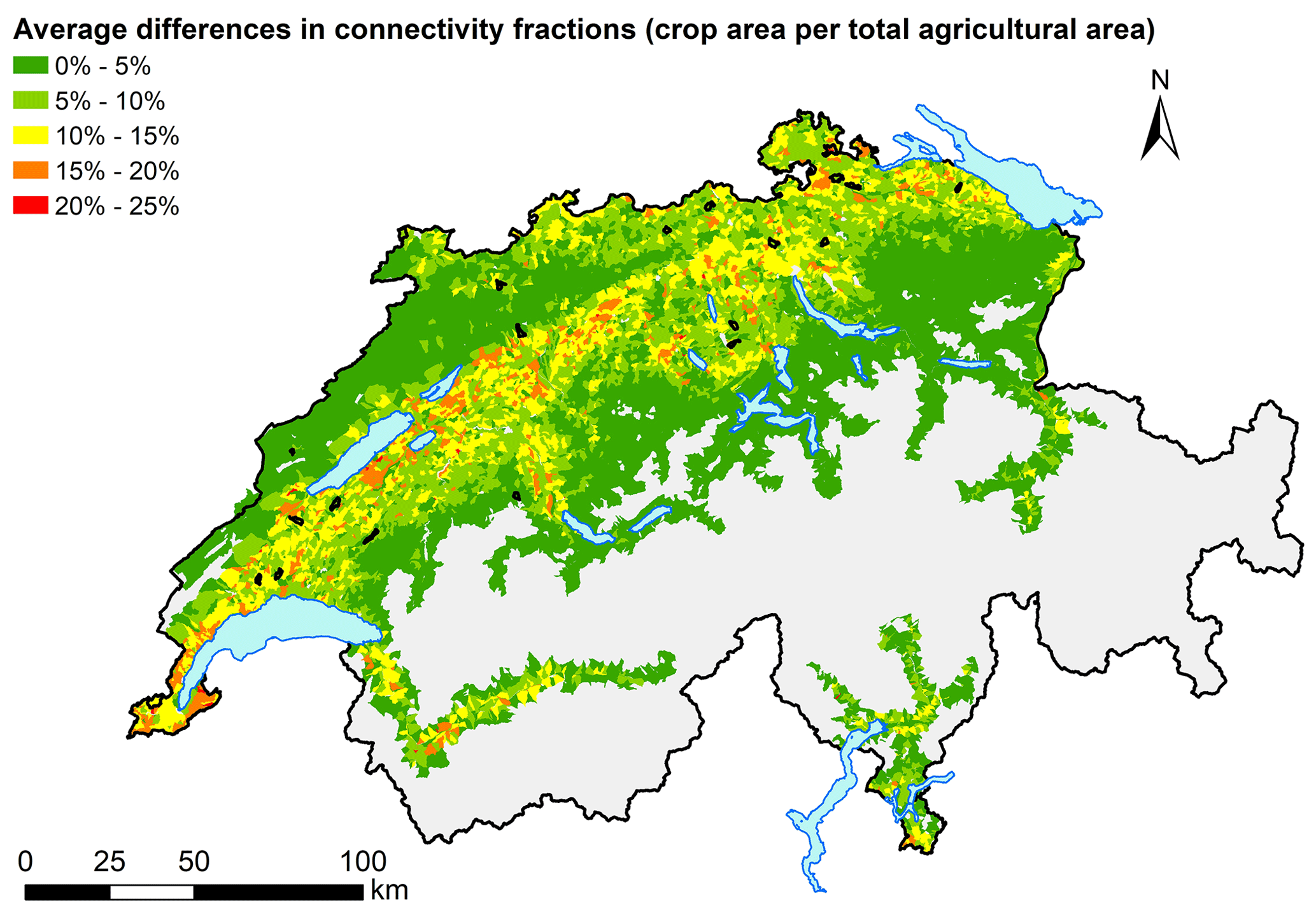
Figure 8 Average differences in connectivity fractions of crop areas between the NSCM and the NECM, as follows: $\mathrm{\Delta }{f}_{\mathrm{crop}}=\left(\right(f_{\mathrm{NSCM},\mathrm{crop},\mathrm{dir}}-f_{\mathrm{NECM},\mathrm{crop},\mathrm{dir}})+(f_{\mathrm{NSCM},\mathrm{crop},\mathrm{indir}}-f_{\mathrm{NECM},\mathrm{crop},\mathrm{indir}})+(f_{\mathrm{NSCM},\mathrm{crop},\mathrm{nc}}-f_{\mathrm{NECM},\mathrm{crop},\mathrm{nc}}\left)\right)/\mathrm{3}$. The map shows data for all Swiss catchments in the valley zones, hill zones, and lower elevation mountain zones. Grey areas represent higher elevation mountain zones that were excluded from the analysis. Study areas are marked with black lines. Details on directly, indirectly, and not connected agricultural areas and crop areas are given in Figs. S37 to S43. For comparison, a map of crop densities is given in Fig. S29. Source of background map: Swisstopo (2010).

4 Discussion

4.1 Occurrence of hydraulic shortcuts

Our study shows that storm drainage inlet and maintenance shafts are common structures found in Swiss agricultural areas. While in neighbouring countries roads are often drained by ditches, Swiss roads are usually drained by storm drainage inlet shafts (Alder et al., 2015). It is, therefore, not surprising that most of the inlet shafts found in the study areas are located on roads. These findings are in accordance with the only other study in Switzerland reporting numbers on storm drainage inlet shafts (Prasuhn and Grünig, 2001).

The vast majority of mapped storm drainage inlet shafts were found to discharge to surface waters directly or via wastewater treatment plants (WWTPs). Thus, the occurrence of an inlet shaft is, in most cases, directly related to a risk for pesticide transport to surface waters. The following three processes generate this risk. First, pesticide-loaded surface runoff produced on crop areas can enter the inlet shaft. Second, spray drift deposited on roads can be washed off and enter the inlet shaft. Third, inlet shafts can be oversprayed during pesticide application, which is mainly considered probable for inlet shafts located in the fields.

Although maintenance shafts were also found to discharge to surface waters directly or via WWTPs, their occurrence does not directly translate into a risk for pesticide transport to surface waters. In contrast to storm drainage inlet shafts, maintenance shafts are not designed to collect surface runoff. Their lids are usually closed or only have a small opening, significantly decreasing the risk of either surface runoff entering the maintenance hole or of overspraying. In addition, lids of maintenance shafts in fields are often elevated compared to the soil surface. Maintenance shafts on roads are (in contrast to inlet shafts) usually positioned so that concentrated surface runoff bypasses them. However, as also shown by Doppler et al. (2012), maintenance shafts can collect surface runoff from fields if they are located in a sink or a thalweg and water is ponding above them during rain events. During our field mapping campaign, we additionally found several damaged maintenance shafts that could easily act as a shortcut.

Channel drains and ditches discharging into surface waters were rare in most study areas, with two exceptions. In Meyrin, the large length of these structures can be explained by the existence of a large vineyard. Additionally, the shaft density in this vineyard was higher than on the surrounding arable land. This indicates that vineyards could generally have higher shortcut densities than arable land. In Buchs, around 60 % of the channel drain and ditch length consists of ditches that cannot be clearly distinguished from small streams. They are not appearing in the national topographic landscape model (Swisstopo, 2010) that was used for the definition of rivers and streams and did not appear to be streams during field mapping or when analysing aerial images.

The number of mapped shortcuts represents a lower boundary estimate of the shortcuts present (see Sect. 3.1.3) and, therefore, leads to an underestimation of indirect connectivity. Probabilities for missing shortcuts during our mapping campaign depend on their location. While aerial images were at almost full coverage of the study areas, field mapping was performed mainly along roads. Drainage plans were available more often along roads than on fields. Therefore, we expect that the detection probability of shortcuts is generally higher along roads than on fields. Besides coverage, various other factors influence the detection probabilities of the mapping methods. Field mapping and aerial image detection performance is reduced if shortcuts are covered. Along roads, this is mainly caused by leaves, soil, and, for aerial images, also by trees and vehicles. On the fields, this is mainly caused by soil or by crops. Detection performance of the aerial images method is additionally influenced by image quality and ground resolution. Image quality is mainly influenced by wind and light conditions during the UAV flights. In order to ensure high image quality, we planned UAV flights for favourable weather conditions (low wind and slightly overcast). However, differences in image quality between the study areas could not be completely avoided. Higher ground resolution could further improve the data produced. Although detection performance is not expected to be limited by the ground resolution used, higher resolution could improve the correct classification of shortcut types.

4.2 Surface runoff connectivity

Our study suggests that around half of the surface runoff connectivity in our study areas, but also on the national scale, is generated by hydraulic shortcuts. Surface runoff is considered one of the most important processes for pesticide transport to surface waters. Consequently, a large amount of the pesticide loads found in surface waters during rain events is expected to be transported by hydraulic shortcuts. These findings are in accordance to the results of other studies investigating the influence of hydraulic shortcuts on surface runoff connectivity (Alder et al., 2015; Prasuhn and Grünig, 2001; Bug and Mosimann, 2011; Remund et al., 2021) and on pesticide transport (Doppler et al., 2012).

The fraction of indirect connectivity was found to be very different between study areas. The variability introduced by the different properties of the study areas was larger than the variability introduced by the different model parameters of the Monte Carlo analysis, indicating that our results are robust against changes in our model parameters. Our model was most sensitive to changes of the parameters road carving depth, shortcut definition, and sink depth. These parameters are discussed in the following.

The parameter road carving depth accounts for the property of roads of collecting and concentrating surface runoff. This effect is strongly dependent on microtopography, is extremely variable in space, and can therefore not be properly accounted for by a space-independent parameter. Usage of a higher resolution digital elevation model could, however, reduce the uncertainty on the effect of roads on connectivity. Higher resolved digital elevation models could also help in capturing the influence of other microtopographical features better. For example, small ditches or small elevations on the ground can easily channel surface runoff. This can either direct surface runoff into a shortcut from areas not modelled to drain to a shortcut or vice versa. In Switzerland, a new digital elevation model with a raster resolution of 0.5 m (Swisstopo, 2019) recently became available and could be used for this purpose. This elevation model was not used in this study, since the study already had progressed further by the time the data set was published.

The model parameters shortcut definition (i.e. maintenance shafts in a sink considered as being a shortcut) and sink depth are both related to the fate of surface runoff ponding in a sink. This indicates that maintenance shafts in sinks could have an important influence on surface runoff connectivity of agricultural areas. During our field mapping campaign, only a few maintenance shafts in sinks were investigated. It is, therefore, unclear if most maintenance shafts in sinks are capturing ponding surface runoff, if surface runoff is usually infiltrating into the soil, or if it continues to flow on the surface. Sensitivity of our model to the parameter sink depth additionally indicates that sinks might play an important role for connectivity. Therefore, they should not be filled completely during a geographic information system (GIS) analyses, as this is done by default by some flow routing algorithms.

Surface runoff is usually assumed to drain to the receiving water of its topographical catchment. However, in various cases, the pipes draining hydraulic shortcuts were found to cross topographical catchment boundaries. Consequently, surface runoff and related pesticide loads are transported to a different receiving water than expected by the topographical catchment. This may be important to consider when interpreting pesticide monitoring data from small catchments. Similar effects were already reported for karstic aquifers or the storm drainage systems of urban areas (Jankowfsky et al., 2013; Luo et al., 2016).

4.3 Hydrological activity

We did not find any indication on systematic differences between the factors controlling hydrological activities of directly and indirectly connected agricultural areas by analysing the slope and topographic wetness index. Those variables are proxies for surface runoff formation, soil moisture, groundwater level, and also physical properties of the soil (Sorensen et al., 2006; Ayele et al., 2020). However, the hydrological activity of an agricultural area also depends on other factors that were not quantitatively analysed, such as rainfall intensities, crop types, soil management practices, or the presence of tile drainage systems.

Rainfall intensities. Because of the small size of the study areas and the close proximity between directly and indirectly connected areas, systematic differences in rainfall intensities within a catchment can be excluded.

Crop types and soil management. These variables can have a strong impact on runoff formation. They are chosen by the farmers, and there could be systematic differences in these variables. For example, farmers aware of the effect of surface runoff and erosion on the pollution of surface waters might use different cultivation methods or crops (e.g. conservation tillage) on fields close to surface waters than on fields far away. This would lead to a higher probability of surface runoff formation on indirectly connected areas compared to directly connected areas. However, different cultivation methods require different farm machinery. Therefore, cultivation methods are often constrained by the machinery available, and farmers use the same cultivation method per crop for all of their fields. Consequently, systematic differences in crop types or soil management between directly and indirectly connected areas of a catchment are unlikely.

Tile drainage systems. Inlet and maintenance shafts found in the field often belong to a tile drainage system. Therefore, fields on which such shafts are located have a higher probability to be drained by tile drainage systems than other fields. This could lead to higher infiltration capacities and, consequently, to reduced surface runoff on indirectly connected areas compared to directly connected areas. However, since most of the inlet and maintenance shafts are located along roads (see Sect. 3.1.1), such differences would only have a minor effect on the overall surface runoff connectivity.

Although rainfall intensities, crop types, and soil management practices are not expected to differ systematically within a catchment, they do differ across catchments. As mentioned in the results, we, therefore, expect the proportion of directly connected areas to indirectly connected areas in a catchment to be a good indicator for the proportion of surface runoff formed on directly and indirectly connected areas in this catchment. However, due to differences in hydrological activity, two catchments with similar total connected areas may differ strongly in the total amount of surface runoff formed.

4.4 Extrapolation to the national level

A major source of uncertainty in the national erosion connectivity model (NECM) is the usage of generalizing assumptions due to a lack of empirical data. Our results show that some of the estimated connectivity fractions of crop areas change significantly when the NECM is transformed based on additional empirical data from our field study. However, the results of both models still are in the same order of magnitude and lead to the same general conclusion. At the national level, more than half of the connected crop area is connected to surface waters via hydraulic shortcuts, as we observed for the 20 study catchments. As shown in Sect. 3.2.4, large differences between the NECM and the NSCM in the predictions of crop area connectivity are almost exclusively found in one band of catchments with high cropping densities in the Swiss midland. Potential further empirical investigations or improvements of the NECM should, therefore, focus on a better representation of these catchments.

However, it is important to note that, within this study, none of the models (NECM, LSCM, and NSCM) has been tested and validated empirically with independent data regarding their actual capacity to quantify the connectivity effects on surface runoff and related pesticide transport. These models provide predictions given the current availability of empirical observations. Suggestions for validating these models are given in Sect. 4.7.

From all tested variables, the NECM connectivity fractions showed the strongest correlations to the connectivity fractions reported by the local connectivity model (LSCM) in our study areas. This suggests that the NECM is a useful tool for assessing potential pesticide connectivity in relative terms (e.g. which catchments have high indirect connectivity compared to other catchments). Therefore, we recommend continuing to use the NECM in practice, for example, as a starting point for identifying hotspot catchments of direct or indirect connectivity. Since the model results are not validated with independent data, they should always be combined with a verification in the field.

To create the NSCM, all crop areas on which pesticides are commonly applied (arable land, vineyards, orchards, and horticulture) were assumed to contribute by the same amount to the pesticide transport via surface runoff. However, these crop types are known to differ in the amounts of pesticide applied (De Baan et al., 2015), in the amounts of surface runoff produced, and also with respect to their connectivity to surface waters. This assumption could, therefore, be refined by considering pesticide application data and by investigating surface runoff connectivity in vineyards, orchards, and horticulture in more detail.

4.5 Relevance in a broader geographical context

This study focussed on the relevance of hydraulic shortcuts in Switzerland. To our knowledge, no studies have systematically analysed the occurrence of hydraulic shortcuts in other countries. Nevertheless, the available literature suggests that, in some regions, such artificial structures like roads, pipes, or ditches are important for connecting fields with the stream network. For example, this was reported in the regions of Alsace (France; Lefrancq et al., 2013), Lower Saxony (Germany; Bug and Mosimann, 2011), Baden-Württemberg (Germany; Gassmann et al., 2012), and Rhineland-Palatinate (Germany; Rübel, 1999). Based on our findings, we hypothesize that shortcuts are mainly important in areas with small field sizes. This increases the density of linear structures, such as roads, for access.

4.6 Implications for practice

In Swiss plant protection¹ legislation and authorization, the effect of hydraulic shortcuts on pesticide transport is currently not considered. Pesticide application is prohibited within a buffer of 3 m along open water bodies, and according to the Swiss proof of ecological performance (PEP), vegetated buffer strips have to be at least 6 m wide. In contrast, along roads, a buffer of only 0.5 m is required. Hence, the current Swiss legislation is protecting surface waters against direct, but not against indirect, transport. This contrasts with the results of this study, suggesting that approximately half of the surface runoff related pesticide transport is occurring indirectly. This implies that there is evidence of a systematic gap in understanding and regulating pesticide risk at the national scale. The same gap was already pointed out by Alder et al. (2015) for soil erosion. However, beyond anecdotal evidence (e.g. Doppler et al., 2012), this gap has not yet been validated with independent measurements of surface runoff and pesticide transport in the field.

While there remain important scientific questions about the validation of the suggested gap, authorities may wish to decide on mitigation measures despite such uncertainties. We, therefore, elaborate on potential mitigation measures in the following.

The most evident measures, based on the current legislation, are vegetated buffer strips along drained roads and around hydraulic shortcuts, infiltrating surface runoff before it reaches a shortcut. Generally, measures increasing infiltration capacity on the field would reduce pesticide transport. Other measures could aim at the shortcut structures themselves (e.g. construction of shortcuts as small infiltration basins, removal of shortcuts, or treatment of water in shortcuts) or on the pipe outlets (e.g. drainage of shortcuts to infiltration basins or treatment of water at the pipe outlet).

Finally, pesticide transport via hydraulic shortcuts could be incorporated into the registration procedure and be considered for the mandatory mitigation measures that go with a registration. Models used in this context are currently only considering transport via direct surface runoff, erosion, tile drainages, and spray drift (De Baan, 2020).

4.7 Further research

Model validation. The model estimations presented here can give insight on pesticide transport via hydraulic shortcuts on the catchment and the national scale. However, as pointed out above, these models lack a field validation with independent measurements on flow and pesticide transport. In the following, we suggest validation approaches to overcome this limitation.

In our opinion, a validation of the local surface runoff connectivity model is ideally performed by measuring runoff and pesticide transport in a set of different small catchments. This should be done along a gradient of ratios between indirectly and directly connected areas (see Fig. 6). Ideally, the catchments should be similar with respect to their structure (e.g. size, stream length, slope, land use, climate, and soil properties). Signals measured at the catchment outlet are always a superposition of different flow pathways. Therefore, runoff and pesticide transport through hydraulic shortcuts cannot be directly measured at the catchment outlet. To disentangle transport through hydraulic shortcuts from other pathways, we foresee two different approaches.

The first approach aims to observe flow and transport within a catchment at locations where an unambiguous differentiation between the flow paths is possible. For example, hydraulic shortcuts in a catchment could be equipped with a discharge measurement and a water sampler. Such a set-up would allow us to determine the proportion of total catchment runoff and pesticide load that is transported via hydraulic shortcuts. In addition, isotopic tracers and runoff separation techniques could be used to determine the total amount of surface runoff contributing to catchment runoff. If the model is valid, the ratio of measured direct to measured indirect surface runoff should be proportional to the ratio of directly to indirectly connected areas. Additionally, these measurements could be used to improve the parameterization of the local connectivity model.

However, due to the large numbers of measurement locations needed, the above-mentioned validation approach would be very laborious. The second validation approach, therefore, aims to disentangle transport through hydraulic shortcuts while only measuring at the catchment outlet of a set of catchments. For the interpretation of the local connectivity model, we assumed that direct and indirect surface runoff are proportional to the directly and indirectly connected area. If this assumption is valid, more surface runoff should reach the stream in catchments with larger fractions of connected areas. Consequently, in such catchments, runoff coefficients should be higher during discharge events that are predominantly triggered by Hortonian overland flow, such as intensive thunderstorms. For these events, uncertainties introduced by different subsurface properties of the catchments play a minor role compared to other events. Furthermore, if a set of catchments has similar fractions of directly connected area, but different fractions of indirectly connected area, then larger runoff coefficients should be measured in catchments with larger fractions of indirectly connected area.

If the local connectivity model proves valid on the catchment scale, the question would be how to improve on the spatial extrapolation to the national scale. Except for the occurrence of hydraulic shortcuts, all input data for the local connectivity model are available on this larger scale as well. Therefore, the local connectivity model can easily be extended to much larger scales if the occurrence of hydraulic shortcuts is known. However, the shortcut mapping procedure used in this study is time-consuming. Thus, to efficiently map shortcuts on larger scales, automated algorithms for shaft localization, using remote sensing data, could be used (e.g. Mattheuwsen and Vergauwen, 2020; Moy de Vitry et al., 2018). An application of the local connectivity model to larger scales could then replace the extrapolation approach used in this study, eliminating the associated uncertainty.

Shortcuts in vineyards. Our results (i.e. Meyrin and additional field observations) suggest that the presence of hydraulic shortcuts and the fraction of indirectly connected areas are higher in vineyards than on arable land. Since this study focused mainly on the latter, the sample size was too small for a quantitative analysis of vineyards. The fact that Swiss vineyards usually have high road densities points in the same direction. In Swiss vineyards, pesticides are applied more often and in larger amounts than on arable land (De Baan et al., 2015). Therefore, an assessment of the hydraulic shortcut relevance in vineyards is needed.

Spray drift on roads. Hydraulic shortcuts are not only collecting surface runoff from target areas but also from non-target areas such as roads. As shown by Lefrancq et al. (2013), large amounts of spray drift can be deposited on roads. These deposits are expected to be washed off during rain events and to be transported to surface waters via hydraulic shortcuts. Further research is needed to quantify the relevance of this process for pesticide pollution in streams.

Hydrological activity. In our discussion on hydrological activity (see above), we explained that systematic differences in hydrological activity are unlikely within a catchment but are expected across catchments. Further research should aim to quantify the differences in hydrological activity across catchments and their influence on runoff formation. Some of the data sets that could serve such a comparison are available on the national scale, e.g. a map of tile drainage potential (Koch and Prasuhn, 2020) or rainfall statistics (e.g. Hydrological Atlas of Switzerland, 2018). Other data sets are currently being developed (e.g. a national, plot-specific crop-type data set) or have to be developed (e.g. national soil maps).

5 Conclusions

Our study shows that hydraulic shortcuts are common structures found in Swiss arable land areas of the Swiss plateau. Shortcuts are found mainly along roads but also directly in the field. The analyses suggests that, on average, around half of the surface runoff connectivity on Swiss arable land is caused by hydraulic shortcuts. Further analyses on hydrological activity and crop density suggest that the same proportion of surface runoff and related pesticide load is transported to surface waters through hydraulic shortcuts. This statement holds for both the selected study catchments and the whole country. However, in Swiss pesticide legislation and pesticide authorization, hydraulic shortcuts are currently not considered. Therefore, current regulations may fall short in addressing the full extent of the problem.

The field data acquired in this study suggest that the national erosion connectivity model (NECM) is a useful tool for relatively comparing potential pesticide connectivity between catchments. However, the results also show that additional field data significantly changed the reported connectivity fractions and improved the model reliability.

Overall, the findings highlight the relevance of better understanding the connectivity between fields and the receiving water as well as the underlying factors and physical structures in the landscape. The model results of this study lack validation with field measurements on actual water flow and pesticide transport in hydraulic shortcuts. This should be addressed in further research. Propositions for such validations are presented in Sect. 4.7.

This study focused on the contribution of hydraulic shortcuts to surface runoff connectivity and related pesticide transport on arable land. However, for other crop types, the contribution of shortcuts is expected to be different. Especially in vineyards, we expect a higher contribution due to their spatial structure (e.g. high road densities or steep slopes) and due to higher pesticide use.