Physical versus economic water footprints in crop production: a spatial and temporal analysis for China

A core goal of sustainable agricultural water resources management is to implement a lower water footprint (WF), i.e. higher water productivity, and to maximize economic benefits in crop production. However, previous studies mostly focused on crop water productivity from a single physical perspective. Little attention is paid to synergies and trade-offs between water consumption and economic value creation of crop production. Distinguishing between blue and green water composition, grain and cash crops, and irrigation and rainfed production modes in China, this study calculates the production-based WF (PWF) and derives the economic value-based WF (EWF) of 14 major crops in 31 provinces for each year over 2001–2016. The synergy evaluation index (SI) of PWF and EWF is proposed to reveal the synergies and trade-offs of crop water productivity and its economic value from the WF perspective. Results show that both the PWF and EWF of most considered crops in China decreased with the increase in crop yield and prices. The high (low) values of both the PWF and EWF of grain crops tended to cluster obviously in space and there existed a huge difference between blue and green water in economic value creation. Moreover, the SI revealed a serious incongruity between PWFs and EWFs both in grain and cash crops. Negative SI values occurred mostly in north-west China for grain crops, and overall more often and with lower values for cash crops. Unreasonable regional planting structure and crop prices resulted in this incongruity, suggesting the need to promote regional coordinated development to adjust the planting structure according to local conditions and to regulate crop prices rationally.

1 Introduction

Humanity is facing the increasingly severe threat of water shortage and accompanying rising food risks (Mekonnen and Hoekstra, 2016; Veldkamp et al., 2017), posing great challenges to agricultural water resource management. The economic benefits of water use form one important pillar of fresh water distribution (Hoekstra, 2014). However, traditional studies on efficient agricultural water use focus on crop water productivity from the physical perspective and rarely make comprehensive evaluations combining the results with an economic perspective. The water footprint (WF) (Hoekstra, 2003) reveals the consumption and pollution of water in the process of production or consumption and assesses fresh water appropriation in its entirety (Hoekstra et al., 2011). The consumptive WF of crop production can be divided into blue and green WFs (Hoekstra et al., 2011). Blue water is surface and ground water, whereas green water is defined as the water kept in the unsaturated soil layer and precipitation, which is eventually transferred into canopy evapotranspiration (Falkenmark and Rockstrom, 2006). In agriculture, the blue WF measures irrigation water consumption. Green WF refers to the consumption of rainwater (Hoekstra et al., 2011). As a comprehensive index to evaluate types, quantities, and efficiency of water use in the process of crop production, the WF of crop production can be expressed based on both production (PWF, m³ kg⁻¹) and economic value (EWF, m³  per  monetary  unit) (Garrido et al., 2010; Hoekstra et al., 2011), which unifies the measurement of the physical and economic levels. PWF and EWF provide clear insights for reducing the water resources input for harvesting crop yields and optimizing the economic benefits per unit of water consumption, respectively.

Garrido et al. (2010) firstly evaluated WF in terms of m³ EUR⁻¹, from a perspective of hydrology and economy for the agricultural production of Spain. They found that in areas where blue water was scarce but dominant in crop production, the scarce blue water resource was used to irrigate high-value crops, thus achieving higher yields and economic benefits, with a more efficient blue water utilization with increasing scarcity. In a case study for Kenya, Mekonnen and Hoekstra (2014a) encouraged the use of domestic water resources for production of the rainfed cash crops with high economic benefits, rather than for water-intensive export commodities with low economic benefits. Schyns and Hoekstra (2014) found that water and land resources in Morocco were mainly used to produce export crops with relatively low economic value (in terms of USD m⁻³ and USD ha⁻¹), and that water-scarce countries should attribute great importance to the allocation of freshwater and adjust crop planting structure from the perspective of economic efficiency. Chouchane et al. (2015) quantified the WF in Tunisia and evaluated the blue and green economic water productivity and economic land productivity in irrigation and rainfed agriculture from an economic perspective. They showed that irrigation water was not generally used to increase economic water productivity (USD m⁻³) but rather to increase economic land productivity (USD ha⁻¹), so it would be advantageous to expand the irrigated area of crops with high economic water productivity. Furthermore, in recent years, there have been studies on the dairy industry (Owusu-Sekyere et al., 2017a, b), the meat industry (Ibidhi and Salem, 2018), and the wine industry (Miglietta et al., 2018) to explore the WF assessment combined with an economic perspective.

Nevertheless, the above studies lacked a complete temporal and spatial evolution analysis of the WF from the economic perspective. More importantly, the above studies did not involve the study of WF coordination in different aspects, which means a good synergy in reducing the water resources input for harvesting crop yields and optimizing the economic benefits per unit of water consumption, compared with the national average level. Thus, the synergies and trade-offs between water consumption and economic value creation during crop production in WF assessment, which is undoubtedly of great significance, are ignored.

Scientifically planning agricultural water resource utilization and balancing crop production, water consumption, and social economic development are severe challenges faced by all humankind. However, China, with millions of small farmers led by smallholder production, has become one of the regions facing the biggest challenges (Tilman et al., 2011; Gao and Bryan, 2017; Cui et al., 2018). Being the country with the largest population and food consumption, China faces a series of problems, such as extensive management and low utilization rate of water resources in agricultural production (Khan et al., 2009; Kang et al., 2017). Previous studies on China have quantified the WF of crop production at the irrigation district scale (Sun et al., 2013, 2017; Cao et al., 2014), watershed scale (Zhuo et al., 2014, 2016c) and national scale (Zhuo et al., 2016b; Wang et al., 2019). Sun et al. (2013) found that the WF of crops depended on agricultural management rather than on regional climate differences. Zhuo et al. (2016b) showed that China's domestic food trade was determined by the economy and government policies, not by regional differences in water endowments. Wang et al. (2019) showed possibility and importance of accounting for developments of water-saving techniques in large-scale crop WF estimations. However, most of these studies focused on quantifying WF from a single physical perspective. To our knowledge, there is no study yet to provide clear insights into the economic benefits of water use.

To fill the above research gap, the current study objective is, taking China over 2001–2016 as the study case, to explore the relationship between water resource consumption and economic value creation of intra-national-scale crop production, and to propose a synergy evaluation index (SI) of PWF and EWF to reveal the synergies and trade-offs of crop water productivity and its economic value from the WF perspective. First, the blue and green PWF (PWF_b, PWF_g) of 14 major crops (winter wheat, spring wheat, spring maize, summer maize, rice, soybean, cotton, groundnut, rapeseed, sugar beet, sugarcane, citrus, apple, and tobacco) is calculated annually in 31 provinces at the meteorological station level, and the corresponding EWF is derived. Second, crops are distinguished between grain and cash crops, with the Mann–Kendall trend test and spatial autocorrelation analysis method for evaluation of the temporal and spatial evolution characteristics of PWF and EWF. Finally, the synergy evaluation index is constructed. Consequently, based on the quantification of PWF and EWF, we constructed the synergy evaluation index of water footprints, so that the original intention of the study, which is a comprehensive assessment from the perspective of both physics and economics, can be implemented.

2 Method and data

2.1 AquaCrop modelling

Crop WF per unit mass is defined by the evapotranspiration (ET) and yield (Y) over the growing period (Hoekstra et al., 2011). The AquaCrop model (Hsiao et al., 2009; Raes et al., 2009; Steduto et al., 2009), a water-driven crop water productivity model developed by FAO, is used to simulate the daily green and blue ET and yield Y of 14 crops for each station. The AquaCrop has fewer parameters than other crop growth models and provides a better balance between simplicity, accuracy, and robustness (Steduto et al., 2009). A large number of studies have demonstrated the good performance of AquaCrop in simulating crop growth and water use under different environmental conditions (Abedinpour et al., 2012; Jin et al., 2014; Kumar et al., 2014). Also, there have been a number of studies using AquaCrop to calculate water footprints (Chukalla et al., 2015; Zhuo et al., 2016a, c; Wang et al., 2019). The dynamic soil water balance in the AquaCrop model is shown in Eq. (1):

$$\begin{array}{}\text{(1)}& \begin{array}{rl}{S}_{\left[t\right]}=& S_{[t-\mathrm{1}]}+{\text{PR}}_{\left[t\right]}+{\text{IRR}}_{\left[t\right]}+{\text{CR}}_{\left[t\right]}-{\text{ET}}_{\left[t\right]}\\ & -{\text{RO}}_{\left[t\right]}-{\text{DP}}_{\left[t\right]},\end{array}\end{array}$$

where S_[t] (mm) is the soil moisture content at the end of day t; PR_[t] (mm) is the rainfall on day t; IRR_[t] (mm) is the irrigation amount on day t; CR_[t] (mm) is the capillary rise from groundwater; RO_[t] (mm) is the surface runoff generated by rainfall and irrigation on day t; DP_[t] (mm) is the amount of deep percolation on day t. RO_[t] is obtained through the Soil Conservation Service curve-number equation (USDA, 1964; Rallison, 1980; Steenhuis et al., 1995):

$$\begin{array}{}\text{(2)}& {\text{RO}}_{\left[t\right]}={\displaystyle \frac{({\text{PR}}_{\left[t\right]}-I_a{)}^{\mathrm{2}}}{{\text{PR}}_{\left[t\right]}+S-I_a}},\end{array}$$

where S (mm) is the maximum potential storage, which is a function of the soil curve number; I_a (mm) is the initial water loss before surface runoff; and DP_[t] (mm) is determined by the drainage capacity (${\mathrm{m}}^{\mathrm{3}}{\mathrm{m}}^{-\mathrm{3}}{\mathrm{d}}^{-\mathrm{1}}$). When the soil water content is less than or equal to the field capacity, the drainage capacity is zero (Raes et al., 2017).

AquaCrop model is able to track the daily inflow and outflow at the root zone boundary. On this basis, we use the blue and green WF calculation framework by Chukalla et al. (2015), Zhuo et al. (2016c), and Hoekstra (2019) combined with the model of soil water dynamic balance to separate the daily blue and green ET (mm), as shown in Eqs. (3) and (4):

$$\begin{array}{}\text{(3)}& {\displaystyle }\begin{array}{rl}{S}_{\mathrm{b}\left[t\right]}=& S_{\mathrm{b}[t-\mathrm{1}]}+{\text{IRR}}_{\left[t\right]}-{\text{RO}}_{\left[t\right]}\cdot {\displaystyle \frac{{\text{IRR}}_{\left[t\right]}}{{\text{PR}}_{\left[t\right]}+{\text{IRR}}_{\left[t\right]}}}\\ & -({\text{DP}}_{\left[t\right]}+{\text{ET}}_{\left[t\right]})\cdot {\displaystyle \frac{S_{\mathrm{b}[t-\mathrm{1}]}}{S_{[t-\mathrm{1}]}}},\end{array}\text{(4)}& {\displaystyle }\begin{array}{rl}{S}_{\mathrm{g}\left[t\right]}=& S_{\mathrm{g}[t-\mathrm{1}]}+{\text{PR}}_{\left[t\right]}-{\text{RO}}_{\left[t\right]}\cdot {\displaystyle \frac{{\text{PR}}_{\left[t\right]}}{{\text{PR}}_{\left[t\right]}+{\text{IRR}}_{\left[t\right]}}}\\ & -({\text{DP}}_{\left[t\right]}+{\text{ET}}_{\left[t\right]})\cdot {\displaystyle \frac{S_{\mathrm{g}[t-\mathrm{1}]}}{S_{[t-\mathrm{1}]}}},\end{array}\end{array}$$

where S_b[t] and S_g[t] (mm) respectively represent the blue and green soil water content at the end of day t. According to Siebert and Döll (2010), the maximum soil moisture of rainfed fallow land 2 years before planting is taken as the initial soil moisture for simulation. At the same time, the initial soil water during the growing period is set as green water (Zhuo et al., 2016c).

The blue and green components in DP and ET were calculated per day based on the fractions of blue and green water in the total soil water content at the end of the previous day (Zhuo et al., 2016a), which are shown in Eqs. (5) and (6):

$$\begin{array}{}\text{(5)}& {\displaystyle }{\text{ET}}_{\mathrm{b}\left[t\right]}& {\displaystyle }={\text{ET}}_{\left[t\right]}\cdot {\displaystyle \frac{S_{\mathrm{b}[t-\mathrm{1}]}}{S_{[t-\mathrm{1}]}}},\text{(6)}& {\displaystyle }{\text{ET}}_{\mathrm{g}\left[t\right]}& {\displaystyle }={\text{ET}}_{\left[t\right]}\cdot {\displaystyle \frac{S_{\mathrm{g}[t-\mathrm{1}]}}{S_{[t-\mathrm{1}]}}}.\end{array}$$

Using the normalized biomass water productivity (WP^∗, kg m⁻²), which is normalized for the atmospheric carbon dioxide (CO₂) concentration, the evaporative demand of the atmosphere (ET₀) and crop classes (C₃ or C₄ crops), AquaCrop calculates daily aboveground biomass production (B, kg) from daily transpiration (T_r) and the corresponding daily reference evapotranspiration (ET₀) (Steduto et al., 2009):

$$\begin{array}{}\text{(7)}& B={\text{WP}}^{\ast }\sum {\displaystyle \frac{T_{r\left[t\right]}}{{\text{ET}}_{\mathrm{0}\left[t\right]}}}.\end{array}$$

The crop yield (harvested biomass) is the product of the above-ground biomass (B) and the adjusted reference harvest index (HI₀, %) (Raes et al., 2017).

$$\begin{array}{}\text{(8)}& Y=f_{\text{HI}}{\text{HI}}_{\mathrm{0}}B,\end{array}$$

where the adjustment factor (f_HI) reflects the water and temperature stress depending on the timing and extent during the crop cycle.

2.2 Calculation of production-based water footprint (PWF)

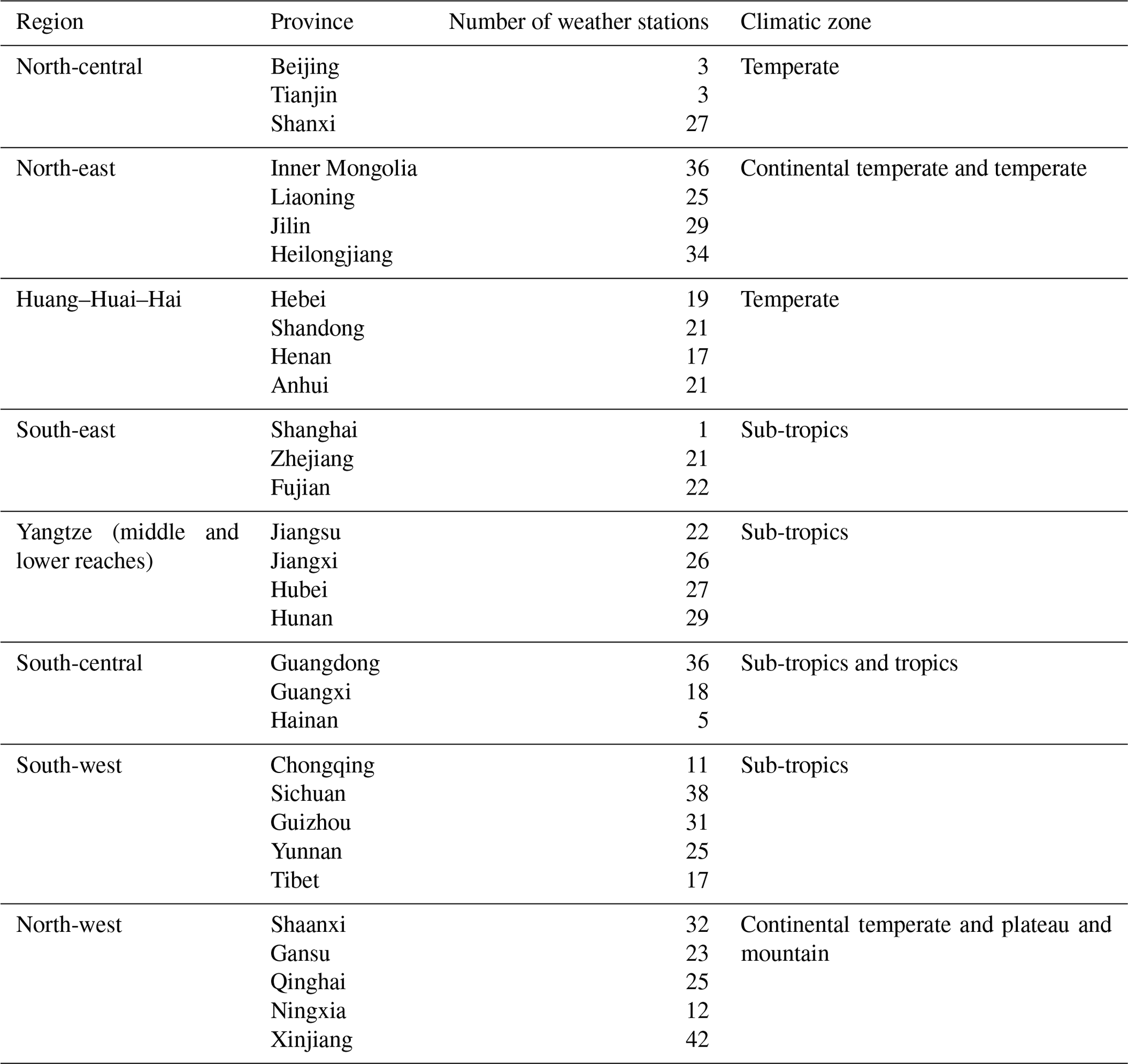
The PWF values of 14 major crops were calculated annually in 31 provinces at the meteorological station level. Table 1 shows the number of meteorological stations per province. The PWF (m³ kg⁻¹) consists of the blue PWF (PWF_b, m³ kg⁻¹) and the green PWF (PWF_g, m³ kg⁻¹), which are respectively calculated from the daily blue evapotranspiration (ET_b[t], mm), daily green evapotranspiration (ET_g[t], mm), and crop yield (Y, kg ha⁻¹) during the growing period (Hoekstra et al., 2011), as shown in Eqs. (9)–(11):

$$\begin{array}{}\text{(9)}& {\displaystyle }& {\displaystyle }\text{PWF}={\mathrm{PWF}}_{\mathrm{b}}+{\mathrm{PWF}}_{\mathrm{g}},\text{(10)}& {\displaystyle }& {\displaystyle }{\mathrm{PWF}}_{\mathrm{b}}={\displaystyle \frac{\mathrm{10}\cdot \sum _{t=\mathrm{1}}^{\text{gp}}{\text{ET}}_{\mathrm{b}\left[t\right]}}{Y}},\text{(11)}& {\displaystyle }& {\displaystyle }{\mathrm{PWF}}_{\mathrm{g}}={\displaystyle \frac{\mathrm{10}\cdot \sum _{t=\mathrm{1}}^{\text{gp}}{\text{ET}}_{\mathrm{g}\left[t\right]}}{Y}},\end{array}$$

where gp (day) is the length of growing period; 10 is the conversion coefficient. The daily ET and Y values during the growth period are simulated by the AquaCrop model. Being consistent with the existing calibration method which has been widely applied (Mekonnen and Hoekstra, 2011; Zhuo et al., 2016c, b, 2019; Wang et al., 2019), the modelled crop yield was calibrated at provincial level according to the statistics (NBSC, 2019). Within a province, we calibrated the average level of the modelled yields among station points to match the provincial statistics. Therefore, we kept the spatial variation in crop yields, so that in associated water footprints could be simulated by the AquaCrop model.

Table 1 Number of meteorological stations per province.

2.3 Calculation of economic value-based water footprint (EWF)

Following Hoekstra et al. (2011), the EWF (m³ USD⁻¹) of crop production represents the water consumption per unit of economic value.

$$\begin{array}{}\text{(12)}& \text{EWF}={\displaystyle \frac{\text{PWF}}{\text{UP}}},\end{array}$$

where PWF (m³ kg⁻¹) is the production-based WF, and UP (USD kg⁻¹) is the crop unit price. The economic benefit unit refers to crop price in the current study. The EWF is numerically equal to the inverse of the economic water productivity. Considering the PWF and the EWF together provides a clear and intuitive measurement to analyse the synergy relationship between water consumption of crop production and economic value creation. To eliminate the influence of inflation, we use the consumer price index (CPI) to calculate the inflation rate of China based on 2001 and to convert the annual crop current price into the 2001 constant Chinese Yuan price (constant 2001 CNY). Then, we convert it to the 2001 constant American dollar price (constant 2001 USD).

Referring to Chouchane et al. (2015), when calculating the blue and green EWF, we distinguish between irrigation and rainfed agricultural modes. In rainfed agriculture, the green EWF (EWF_g,rf) is obtained by dividing the green water consumption per unit yield under rainfed condition by the unit price of crops, as shown in Eq. (13). Compared to rainfed agriculture, the ratio of crop yield increment under full irrigation is obtained by the AquaCrop model. We use it to distinguish the blue and green EWF in irrigation agriculture (EWF_b,ir, EWF_g,ir), as shown in Eqs. (14)–(16):

$$\begin{array}{}\text{(13)}& {\displaystyle }& {\displaystyle }{\mathrm{EWF}}_{\mathrm{g},\mathrm{rf}}={\displaystyle \frac{{\mathrm{CWU}}_{\mathrm{g},\mathrm{rf}}}{Y_{\text{RF}}\cdot \text{UP}}},\text{(14)}& {\displaystyle }& {\displaystyle }\mathit{\alpha }={\displaystyle \frac{Y_{\text{IR}}-Y_{\text{RF}}}{Y_{\text{IR}}}},\text{(15)}& {\displaystyle }& {\displaystyle }{\mathrm{EWF}}_{\mathrm{b},\mathrm{ir}}={\displaystyle \frac{{\mathrm{CWU}}_{\mathrm{b},\mathrm{ir}}}{Y_{\text{IR}}\cdot \text{UP}\cdot \mathit{\alpha }}},\text{(16)}& {\displaystyle }& {\displaystyle }{\mathrm{EWF}}_{\mathrm{g},\mathrm{ir}}={\displaystyle \frac{{\mathrm{CWU}}_{\mathrm{g},\mathrm{ir}}}{Y_{\text{IR}}\cdot \text{UP}\cdot (\mathrm{1}-\mathit{\alpha })}},\end{array}$$

where CWU_g,rf (m³ ha⁻¹) represents the consumption of green water per unit area in rainfed agriculture; CWU_b,ir (m³ ha⁻¹) and CWU_g,ir (m³ ha⁻¹) represent the consumption per unit area in irrigation agriculture of blue and green water, respectively; α is the ratio of crop yield increment under full irrigation obtained by the AquaCrop model; and Y_RF (kg ha⁻¹) and Y_IR (kg ha⁻¹) represent the simulated crop yield after calibration at provincial level under the rainfed and irrigation modes, respectively. The EWF_g,rf represents the amount of green water consumption per economic benefit unit in rainfed agriculture (also refers to the amount of green water input for each additional economic benefit unit); EWF_b,ir (EWF_g,ir) refers to the additional amount of blue (green) water for each additional unit economic benefit under the same green (blue) water input in irrigation agriculture.

2.4 Spatial and temporal evolution of WFs

The Mann–Kendall (M–K) trend test (Mann, 1945; Kendall, 1975) is used to test the annual variation trend of WF of crop production from 2001 to 2016. When using the M–K test for trend analysis, the null hypothesis H₀ is the that all variables in WF time series $\mathit{\{}{\text{WF}}_i\mathrm{|}i=\mathrm{1},\mathrm{2},\mathrm{\dots },\mathrm{16}\mathit{\}}$ are independent and identical in distribution, with no variation trend; the alternative hypothesis H₁ is that all i, j≤16 and i≠j in the distribution of WF_i and WF_j are different, with an obvious upward or downward trend in the sequence. The M–K statistic S is shown in Eq. (17):

$$\begin{array}{}\text{(17)}& S=\sum _{i=\mathrm{1}}^{n-\mathrm{1}}\sum _{j=i+\mathrm{1}}^n\text{sgn}({\text{WF}}_j-{\text{WF}}_i),\end{array}$$

where WF_j and WF_i are the data values of year j and i of the WF time series, respectively; n is the length of the data sample, 16; and sgn is sign function, depicted in Eq. (18).

$$\begin{array}{}\text{(18)}& \text{sgn}\left(\mathit{\theta }\right)=\left\{\begin{array}{ll}\mathrm{1}& \mathit{\theta }>\mathrm{0}\\ \mathrm{0}& \mathit{\theta }=\mathrm{0}\\ -\mathrm{1}& \mathit{\theta }<\mathrm{0}\end{array}\right.\end{array}$$

When n≥8, the M–K statistic S roughly follows a normal distribution, whose mean value is zero, and the variance can be calculated by Eq. (19).

$$\begin{array}{}\text{(19)}& \text{Var}\left(S\right)={\displaystyle \frac{n(n-\mathrm{1})(\mathrm{2}n+\mathrm{5})-\sum _{p=\mathrm{1}}^g{t}_p(t_p-\mathrm{1})(\mathrm{2}{t}_p+\mathrm{5})}{\mathrm{18}}},\end{array}$$

where g is the number of tied groups, and t_p is the number of data values in the Pth group (Kisi and Ay, 2014). When n>10, the test statistic Z_c converges to the standard normal distribution, which is calculated by Eq. (20).

$$\begin{array}{}\text{(20)}& Z_{\mathrm{c}}=\left\{\begin{array}{ll}(S-\mathrm{1})/\sqrt{\text{Var}\left(S\right)}& S>\mathrm{0}\\ \mathrm{0}& S=\mathrm{0}\\ (S+\mathrm{1})/\sqrt{\text{Var}\left(S\right)}& S<\mathrm{0}\end{array}\right.\end{array}$$

Using a two-tailed test, when the absolute value of Z_c exceeds 1.96 and 2.58, it means that the significance test of 95 % and 99 % has been passed, respectively. The positive Z_c indicates an upward trend, while a negative value means a downward trend.

The first law of geography states that everything is related, and things close to each other are more relevant (Tobler, 1970). The global and local spatial relevance of WF is expressed by the Moran's I index (Moran, 1950). A positive spatial autocorrelation exists, when the high or low values of the feature variables of adjacent regions show a clustering tendency in space, and a negative spatial autocorrelation means that the value of the feature variables of adjacent regions is opposite to that of the variable of the examined region. The global Moran's I is used to evaluate the overall spatial relevance of WF of crop production, shown in Eq. (21).

$$\begin{array}{}\text{(21)}& I={\displaystyle \frac{n\sum _{i=\mathrm{1}}^n\sum _{j=\mathrm{1}}^n{W}_{ij}({\text{WF}}_i-\stackrel{\mathrm{‾}}{\text{WF}})({\text{WF}}_j-\stackrel{\mathrm{‾}}{\text{WF}})}{\sum _{i=\mathrm{1}}^n({\text{WF}}_i-\stackrel{\mathrm{‾}}{\text{WF}}{)}^{\mathrm{2}}\sum _{i=\mathrm{1}}^n\sum _{j=\mathrm{1}}^n{W}_{ij}}},\end{array}$$

where n is the number of provinces, 31; WF_i is crop WF of province i; $\stackrel{\mathrm{‾}}{WF}$ is the average WF; and W_ij is the spatial weight between the province i and j, which represents the potential interaction forces between the spatial units. When province i and j are adjacent, W_ij=1; when not adjacent, W_ij=0. At the given significance level (0.05 in this study), if the global Moran's I is significantly positive, it indicates that provinces with similar geographical attributes are clustered in space. On the contrary, if the global Moran's I is significantly negative, it means that provinces with different geographical attributes are clustered in space. A local Moran index (LISA) (Anselin, 1995) is used to detect whether there is local clustering of attributes, and the level (high or low) of the WF of a province is shown by the LISA cluster map. The LISA cluster map contains four types (Anselin, 2005): high–high (H-H) and low–low (L-L) indicate that the level (high or low) of WF in this province is consistent with adjacent provinces; high–low (H-L) and low–high (L-H) mean that the level (high or low) of WF in this province is opposite to adjacent provinces. The analysis of spatial autocorrelation can be realized by the GeoDa. The GeoDa is a free software program intended to serve as a user-friendly and graphical introduction to spatial analysis. It includes functionality ranging from simple mapping to exploratory data analysis, the visualization of global and local spatial autocorrelation, and spatial regression. A key feature of the GeoDa is an interactive environment that combines maps with statistical graphics, using the technology of dynamically linked windows. In terms of the range of spatial statistical techniques included, the GeoDa is most similar to the collection of functions developed in the open-source R environment (Anselin et al., 2006).

2.5 The synergy evaluation index (SI) of PWF and EWF

The SI in the current study is the measure of the synergy levels between the PWF and EWF of crops, by summing up their corresponding difference between the water footprint and the base value divided by the range (the maximum minus the minimum) of the water footprint. Here, we adopt the national average level water footprint value as the reference for comparison. The SI is calculated as follows:

$$\begin{array}{}\text{(22)}& \begin{array}{rl}{\text{SI}}_{i,j,c}=& {\displaystyle \frac{{\stackrel{\mathrm{‾}}{\text{PWF}}}_{j,c}-{\text{PWF}}_{i,j,c}}{{\text{PWF}}_{j,c,max}-{\text{PWF}}_{j,c,min}}}\\ & +{\displaystyle \frac{{\stackrel{\mathrm{‾}}{\text{EWF}}}_{j,c}-{\text{EWF}}_{i,j,c}}{{\text{EWF}}_{j,c,max}-{\text{EWF}}_{j,c,min}}},\end{array}\end{array}$$

where ${\text{SI}}_{i,j,c}$ is the synergy evaluation index of PWF and EWF of crop c at province i in year j, and ${\stackrel{\mathrm{‾}}{\text{PWF}}}_{j,c}$ (m³ kg⁻¹) and ${\stackrel{\mathrm{‾}}{\text{EWF}}}_{j,c}$ (m³ USD⁻¹) are the averages at the national level in year j. Obviously, the absolute value of the difference between the WF and their corresponding national average level cannot exceed the maximum minus minimum values. Therefore, the absolute value of SI cannot exceed 2. When the PWF and EWF in a region are both lower than the respective average at the national level, the SI of the region must be positive; when the PWF and EWF in a region are both higher than the respective average at the national level, the SI of the region must be negative. When one is higher and the other is lower than the corresponding average, the SI may be positive or negative, depending on the difference between the provincial value and the national average.

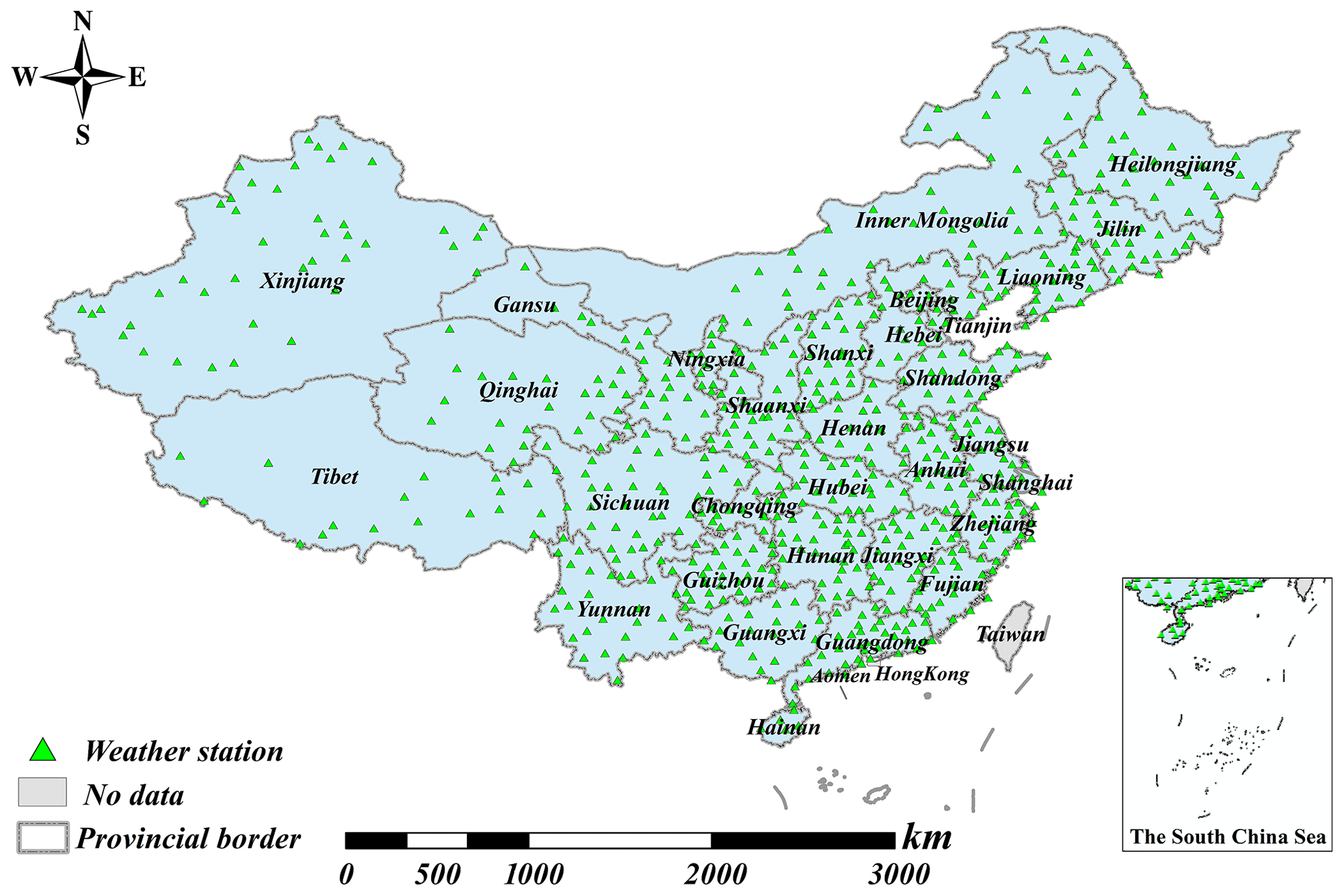
Figure 1 Considered weather stations across mainland China.

2.6 Data sources

The planting area and yield data of each province were obtained from NBSC (2019). The provincial price data of crops were obtained from the China National Knowledge Infrastructure (CNKI, 2019). The current crop prices were converted to the constant prices using the inflation rate based on 2001. The CPI, which is used to calculate the inflation rate, was retrieved from NBSC (2019). The exchange rate used to convert local constant prices into American constant prices was taken from The World Bank (2019). The meteorological data on daily precipitation, daily mean maximum temperature, and daily mean minimum temperature required for the AquaCrop model of 698 meteorological stations in the study area (see Fig. 1) were downloaded from CMDC (2019). The irrigation and rainfed areas of crops were retrieved from MIRCA2000 (Portmann et al., 2010). The soil texture data were taken from the ISRIC database (Dijkshoorn et al., 2008). The soil water content data were from Batjes (2012). The dates of planting of crops referred to Chen et al. (1995). The harvest indexes were taken from Xie et al. (2011) and Zhang and Zhu (1990). Crop growth periods and maximum root depths were taken from Allen et al. (1998) and Hoekstra and Chapagain (2007).

3 Results

3.1 Temporal and spatial evolution of PWF

At the national average level, the PWF of both grain and cash crops showed a significant downward trend over the study period 2001–2016. With the increase in crop yield (grain crop increasing by 26 %, cash crop increasing by 62 %), the PWF of grain crops decreased by 20 % from 1.16 to 0.93 m³ kg⁻¹ (Fig. 2a); and the PWF of cash crops decreased by 35 % from 0.70 to 0.46 m³ kg⁻¹ (Fig. 2b). As for the composition of the WF, the proportion of blue WF of crop production showed a decreasing trend. The proportion of blue WF of grain and cash crops decreased from 39 % and 17 % in 2001 to 34 % and 14 % in 2016, respectively.

Figure 2 Interannual variability of national average production-based water footprint (PWF) of (a) grain and (b) cash crops in China over 2001–2016.

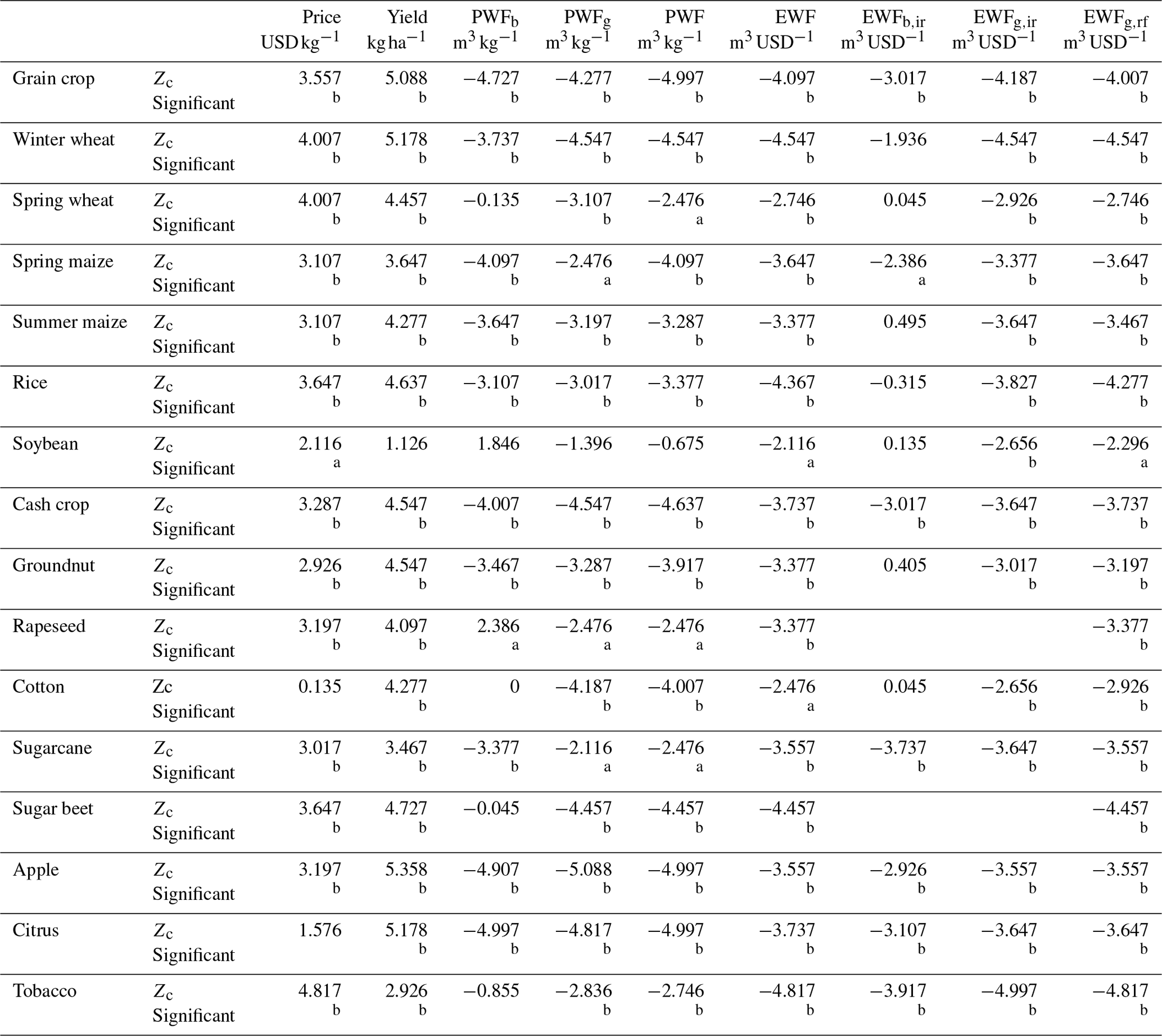
Table 2 lists the PWF, yield, and blue and green water consumption by crops under irrigated and rainfed agriculture in 2001 and 2016. Concerning grain crops, soybean had the highest PWF (2.79 m³ kg⁻¹ in 2016), followed by spring wheat (1.51 m³ kg⁻¹ in 2016). Rice had the lowest PWF (0.78 m³ kg⁻¹ in 2016). Among cash crops, cotton had the highest PWF (3.68 m³ kg⁻¹ in 2016), while sugar beet consumed the least water per yield (0.06 m³ kg⁻¹ in 2016). The proportion of blue WF in spring wheat was the highest (69 % in 2016). Cotton had the highest proportion of blue WF (32 % in 2016) in cash crops. Winter wheat is the grain crop with the highest output in China, and its PWF decreased by 29 % (from 1.47 m³ kg⁻¹ in 2001 to 1.04 m³ kg⁻¹ in 2016). Cotton is the cash crop with the highest water consumption per yield, and its PWF decreased by 31 % (from 5.29 m³ kg⁻¹ in 2001 to 3.68 m³ kg⁻¹ in 2016). The M–K test results of each crop's PWF in Table 3 further confirm the above views. The PWF and yield of different crops had different temporal evolutions. The temporal trends in the PWF_b and PWF_g of the same crop were also different. Among grain crops, winter wheat had the lowest M–K statistical value in PWF (−4.547) and the highest in yield (5.178), jointly showing an obvious positive trend on improving water use efficiency, while the M–K statistic value of soybean was only −0.675, which meant that the PWF of soybean showed little decrease. Soybean planting was dominated by individual farmer mode, with small and fragmented scales and a low planting mechanization degree. Moreover, the harvested area was shrunk (7 202 000 hectares in 2016, 24 % less than 2001). For cash crops, the changes of PWF and yield were most pronounced for fruit crops (apple and citrus). The M–K test result of PWF_b of cotton with the highest water consumption intensity was zero, with almost no changes, given little changes in the yield level in most cotton growing areas.

Table 2 National average production-based water footprint (PWF) and economic value-based water footprint (EWF) of crops in China for the years 2001 and 2016.

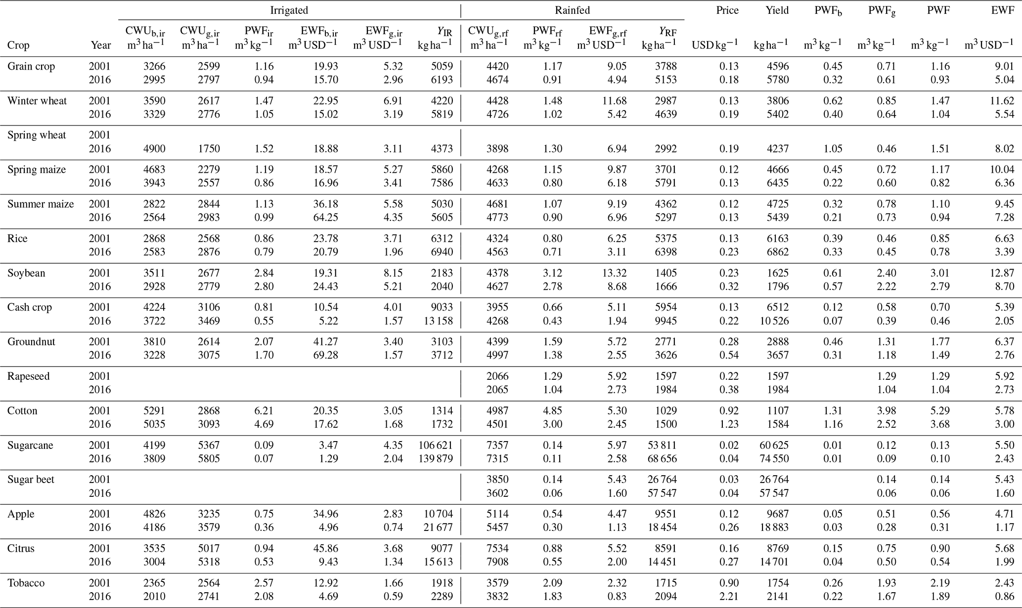
Table 3 M–K analysis of production-based water footprint (PWF) and economic value-based water footprint (EWF) of crops in China.

^a Significant at p<0.05. ^b Significant at p<0.01.

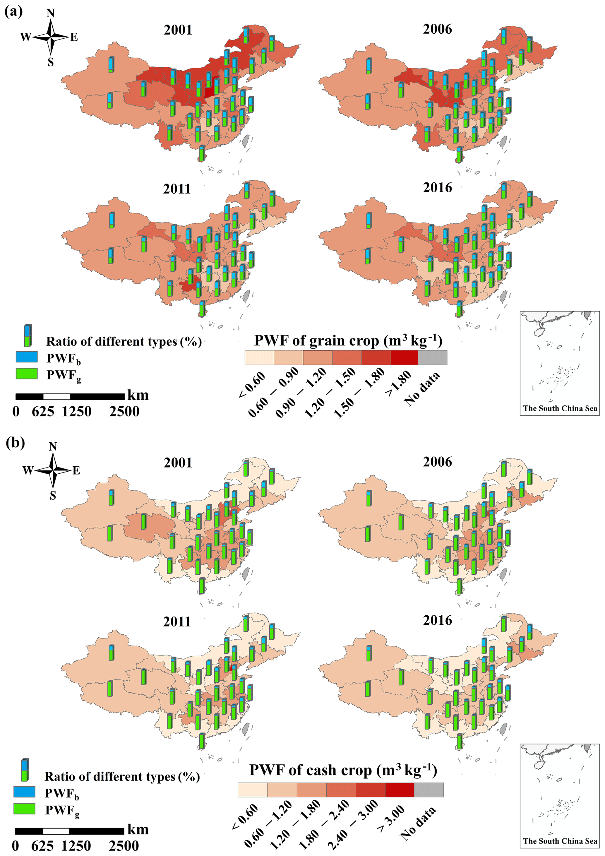
Figure 3 Temporal and spatial evolution of production-based water footprint (PWF) of (a) grain and (b) cash crops in China.

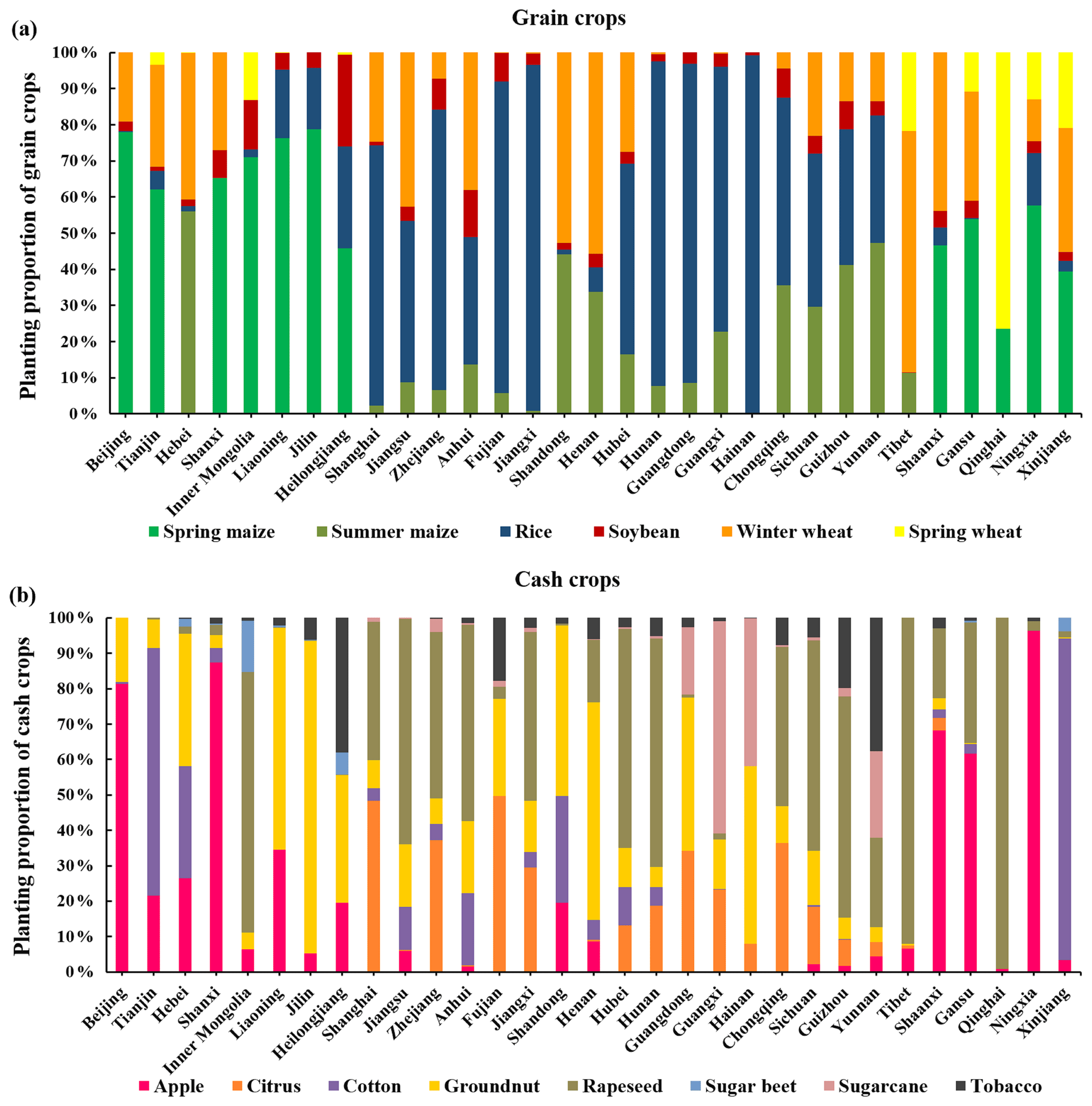
Figure 3a and b shows the spatial distribution of PWF of grain and cash crops across 31 provinces, respectively, in four representative years (2001, 2006, 2011, and 2016). The PWF of grain crops was overall higher in the north-west of China, represented by provinces Shaanxi, Gansu, and Ningxia, with the phenomenon of clustered distribution. The south-eastern coastal areas such as Guangdong, Fujian, and Zhejiang were at a relatively low level. The main reason behind this is that the drier north-west, where wheat and maize grows, has relatively higher evapotranspiration and so higher PWF, while the water-abundant and wet south-east coastal provinces grow rice with a lower PWF. Consistent with the national level analysis, the PWF of the 31 provinces decreased significantly over time (Fig. 3a). Specifically, in north-western China, Gansu province, where the water-intensive wheat and maize were the main grain crops (wheat and maize accounting for 95 % of grain crops in 2016), had the largest grain crop PWF (mean 1.43 m³ kg⁻¹) and showed an obvious downward trend, which decreased by 30 % from 1.73 m³ kg⁻¹ in 2001 to 1.21 m³ kg⁻¹ in 2016. Concerning the composition of blue and green water, Xinjiang had the largest proportion of blue water in grain crops among the 31 provinces, with an annual average of 75 %, far higher than the national average (36 %); the proportion of blue water in grain production in Jilin province was the smallest, with an annual average of 20 %.

Unlike grain crops, the PWF of cash crops was higher in the Beijing–Tianjin–Hebei region, and lower in Inner Mongolia province and the southern areas (Guangdong, Guangxi, and Hainan), without an obvious clustered characteristic (Fig. 3b). This can be interpreted as follows: regarding the cash crops, the dominant crop differs among provinces, which resulted in obvious scattered characteristics in related WFs. For instance, cotton and groundnut with PWF values of 3.68 and 1.49 m³ kg⁻¹ (in 2016) were the leading cash crops in Beijing–Tianjin–Hebei region, whereas rapeseed of lower PWF (1.04 m³ kg⁻¹ in 2016) was the main cash crop in Inner Mongolia. Specifically, during the study period, the PWF of cash crops in Tianjin where cotton was the main cash crop was the largest (3.31 m³ kg⁻¹ in 2011, much higher than the national level of 0.51 m³ kg⁻¹ the same year), with the annual average of 2.90 m³ kg⁻¹. The PWF of cash crops in Guangxi where citrus and sugarcane were dominant was the smallest, with annual average of 0.14 m³ kg⁻¹, much lower than the national level of 0.54 m³ kg⁻¹. Concerning the composition of blue and green water, the proportion of blue water was larger in northern and north-eastern China, and lower in southern and south-western China. Among them, the proportion of blue water of cash crops was the largest in Jilin province, with annual average of 35 %, while the proportion of blue water in Qinghai province was less than 1 %, which was the lowest in China. These results can be explained by the fact that Jilin's main cash crop was groundnut (88 % in 2016), with a high proportion of blue water consumption, while 99 % of Qinghai's cash crops was rainfed rapeseed.

Table 4 Moran's I test for production-based water footprint (PWF) and economic value-based water footprint (EWF) of crop production.

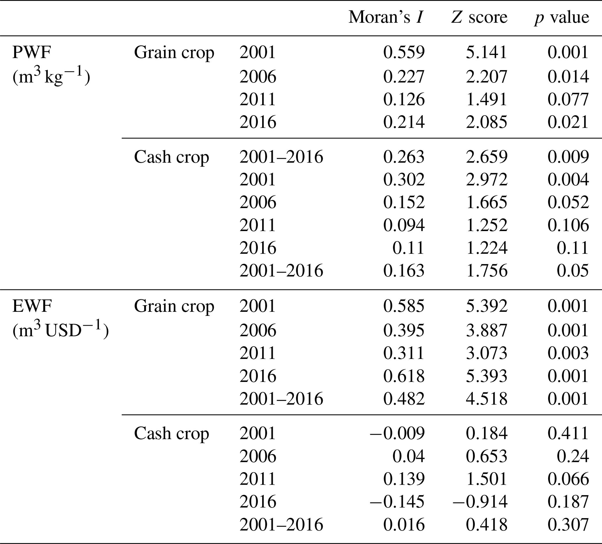
Table 4 shows global Moran's I of PWF of grain and cash crops. The annual average global Moran's I of PWF of grain crops was 0.263, with a clustered spatial distribution in most provinces, and gradually moderated over time (Moran's I decreased from 0.559 in 2001 to 0.214 in 2016). The spatial pattern of PWF of cash crops did not show obvious agglomeration, and the average Moran's I was only 0.163.

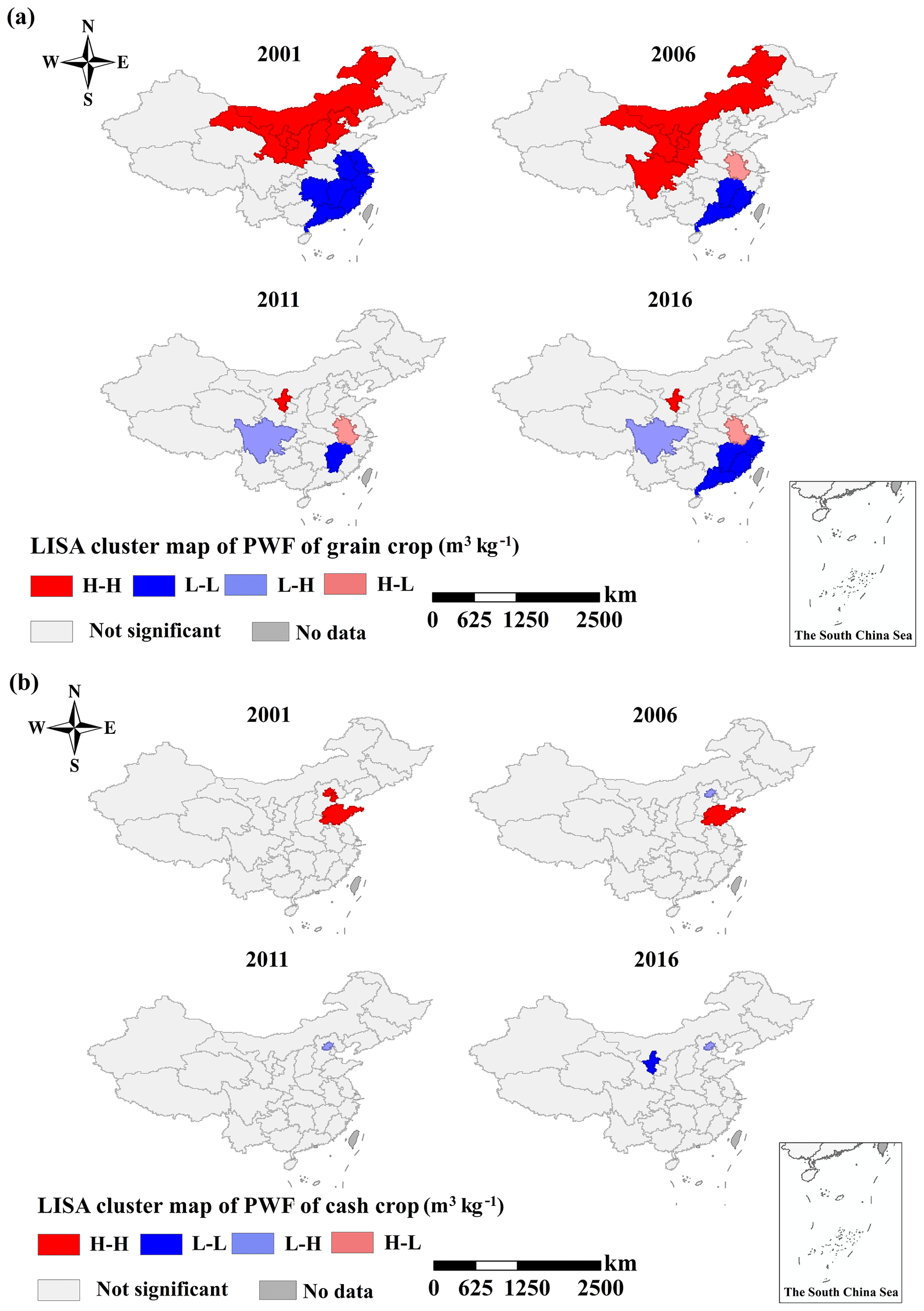
Figure 4 The LISA cluster maps of production-based water footprint (PWF) of (a) grain and (b) cash crops.

The LISA cluster map shows the H-H regions of PWF of grain crops gathered in Gansu, Ningxia, Shaanxi, and Inner Mongolia, and the L-L regions gathered in Guangdong, Zhejiang, Fujian, and Jiangxi (Fig. 4a). At the beginning of the study period, the PWF in 2001 showed an obvious positive spatial correlation, with 13 significant provinces (Gansu, Ningxia, Shaanxi, Shanxi, Inner Mongolia, and Hebei in H-H regions; Guangdong, Zhejiang, Fujian, Jiangxi, Anhui, Jiangsu, and Hunan in L-L regions). In time, the H-H regions in north-western China gradually decreased, leaving only Ningxia in H-H regions, while L-L regions remained relatively stable. Overall, there were seven significant regions in 2016, indicating that the spatial agglomeration of PWF of grain crops decreased with time. This indicates that with the development of water-saving technology and the improvement of agricultural water resource management level, the utilization efficiency of agricultural water resources in the arid north-west region has been gradually improved, while the gap with the more developed and water-rich southern provinces is narrowing. As for cash crops, no obvious agglomeration existed (Fig. 4b).

3.2 Temporal and spatial evolution of EWF

Similar to the evolution of PWF, the EWF of both grain and cash crops showed a significant declining trend at the national average level. With the increase in crop price (grain crop increasing by 40 %, cash crop increasing by 70 %), the EWF of grain crops decreased by 44 %, from 9.01 to 5.04 m³ USD⁻¹ (Fig. 5a); the EWF of cash crops decreased by 62 %, from 5.39 to 2.05 m³ USD⁻¹ (Fig. 5b).

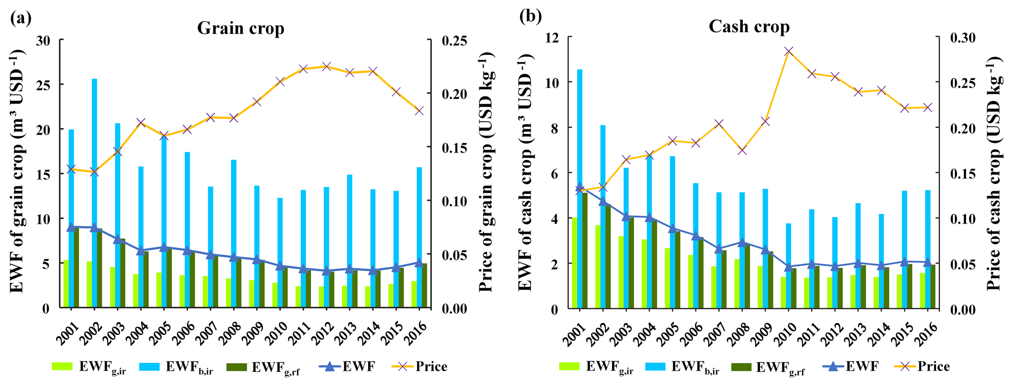
Figure 5 Interannual variability of economic value-based water footprint (EWF) of (a) grain and (b) cash crops in China over 2001–2016.

In terms of grain crops, the EWF_b,ir fluctuated, reaching the highest value of 25.58 m³ USD⁻¹ in 2002 and falling to the lowest of 12.26 m³ USD⁻¹ in 2010. In contrast, the EWF_g,ir and EWF_g,rf showed a significant and steady declining trend, decreasing from 5.32 and 9.05 m³ USD⁻¹ in 2001 to 2.96 and 4.94 m³ USD⁻¹ in 2016, respectively. Among the three types of WF, the EWF_g,ir was the lowest (mean 3.11 m³ USD⁻¹), EWF_b,ir was the highest (mean 15.49 m³ USD⁻¹), and EWF_g,rf (mean 5.31 m³ USD⁻¹) was close to the average EWF (5.41 m³ USD⁻¹) in irrigation and rainfed production modes. This suggests that more water was required per additional benefit unit under irrigation than under rainfed mode, whereas in the irrigated agriculture, compared with blue water, increasing the input of green water may result in more economic benefits. Therefore, utilization efficiency of green water resources for grain crops should be improved.

Concerning cash crops, the EWF_b,ir decreased by 50 % from 10.54 to 5.22 m³ USD⁻¹. Compared to grain crops, the difference between the EWF_g,ir and EWF_g,rf was smaller, with average values of 1.90 and 2.48 m³ USD⁻¹, respectively. In addition, compared to grain crops, the EWF of cash crops was lower, which indicated that cash crop production could get more economic benefits per water consumption unit. Besides, increasing the input of green water resource could obtain higher economic benefits, and the rainfed production had greater economic potential.

Table 2 lists the EWF by crops in 2001 and 2016 at the national scale. Among grain crops, soybean, which consumed the most water per yield unit (2.79 m³ kg⁻¹ in 2016), also had the highest EWF. The second most water-intensive, spring wheat (1.51 m³ kg⁻¹ in 2016), had the second highest EWF (8.02 m³ USD⁻¹ in 2016). Rice, with the lowest water consumption per yield unit (0.78 m³ kg⁻¹ in 2016), also had the lowest EWF (3.39 m³ USD⁻¹ in 2016). Regarding cash crops, cotton, with the highest water consumption per yield unit (3.68 m³ kg⁻¹ in 2016) was the crop with the highest EWF (3.00 m³ USD⁻¹ in 2016). Groundnut's EWF ranked second (2.76 m³ USD⁻¹ in 2016), and sugar beet had lowest water consumption per yield unit (0.06 m³ kg⁻¹ in 2016), with an EWF (1.60 m³ USD⁻¹ in 2016), much lower than the average EWF of cash crops (2.05 m³ USD⁻¹ in 2016).

Sugarcane had the lowest EWF_b,ir (1.29 m³ USD⁻¹ in 2016). The difference between EWF_g,ir and EWF_g,rf of spring wheat was the largest, with 3.11 and 6.94 m³ USD⁻¹, respectively, in 2016. The difference between EWF_g,ir and EWF_g,rf of tobacco was the smallest, with 0.59 and 0.83 m³ USD⁻¹, respectively, in 2016. Table 2 also lists the annual blue and green CWU and yield under irrigated and rainfed conditions by crops in China for the years 2001 and 2016. It can be seen that for all the crops, CWU_g,ir was 21 % (sugarcane) to 55 % (spring wheat) smaller than CWU_g,rf in 2016. Therefore, it is possible that this resulted in EWF_g,ir being much smaller than EWF_g,rf. During the study period, the EWF_g,rf of cash crops decreased most significantly. As for the EWF_b,ir, the downward trend of cash crops was more significant, compared to that of grain crops. The M–K test results in Table 3 further confirmed the above results, as the M–K statistical values of all crops' EWF passed the significance level test of p<0.05. M–K test results for the EWF of most crops were at the similar significance level to that for the corresponding PWF. It is mainly because the M–K test results of the prices of most crops were at the same significant level as the corresponding M–K test results of the yields. Due to the significantly increased price, the EWF M–K test result of soybean was −2.116, which was higher than the test result of corresponding PWF (−0.675). Cotton is another crop worthy of attention. M–K test result for EWF of cotton was −2.476, whose significance level was lower than that of PWF. This is mainly due to fluctuations in the price of cotton. In addition, it can be seen that the changes of EWF_b,ir of most crops were not as obvious as those of EWF_g,ir and EWF_g,ir. It indicates that there is more potential in optimizing the economic benefit of agricultural blue water input.

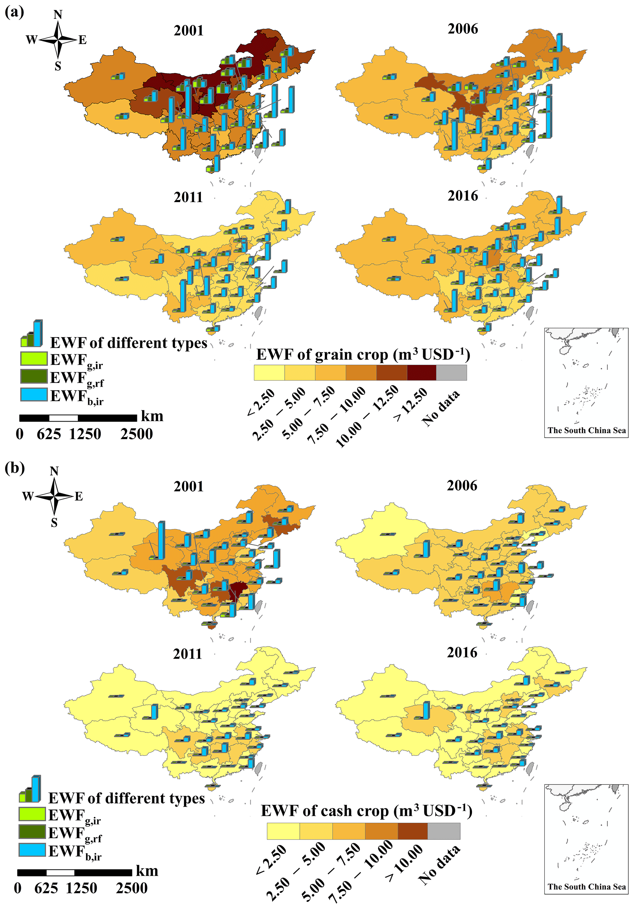
Figure 6 Temporal and spatial evolution of economic value-based water footprint (EWF) of (a) grain and (b) cash crops in China.

Figure 6a and b shows the spatial distribution of EWF of grain and cash crops, respectively. Generally, the EWF of grain crops was higher in Inner Mongolia and north-western China (Shaanxi, Gansu, Ningxia and Xinjiang); Guangdong, Jiangxi, Fujian, Zhejiang, and other south-eastern coastal provinces were at a relatively low level. The north-west, with higher PWF, has lower crop prices due to the relatively underdeveloped economies. In contrast, the economically advanced south-east coastal provinces have both low crop water consumption and higher prices. And the EWF of the 31 provinces showed a significant declining trend over time, which was consistent with the characteristics of the PWF of grain crops above (Fig. 3a). Specifically, Gansu province with the highest PWF of grain crops in north-western China (mean 1.43 m³ kg⁻¹) also had the highest EWF in the top three (mean 8.34 m³ USD⁻¹), with a significant decline of 46 % over time, from 13.28 m³ USD⁻¹ in 2001 to 7.12 m³ USD⁻¹ in 2016. Another high-value area in the north-west is Shaanxi, where winter wheat and spring maize were the main grain crops (44 % and 47 % of all grain crops, respectively, in 2016). The EWF and PWF in Shaanxi (mean 8.15 m³ USD⁻¹ and 1.39 m³ kg⁻¹) were second only to those in Gansu. In contrast, the EWF and PWF (mean 4.49 m³ USD⁻¹ and 0.94 m³ kg⁻¹) in Fujian, with rice as the main grain crop (86 % of all grain crops in 2016), were far lower than the national average (mean 5.41 m³ USD⁻¹ and 1.01 m³ kg⁻¹).

Concerning the composition of blue and green water for grain crops, the EWF_b,ir in north-western China was lower, while the EWF_g,ir and EWF_g,rf were higher. In contrast, the EWF_b,ir in southern China was higher, while the EWF_g,ir and EWF_g,rf were lower. Specifically, in the north-west region, Ningxia had the highest EWF_g,ir and EWF_g,rf (mean 5.25 and 8.35 m³ USD⁻¹, respectively), while the EWF_b,ir was only 7.28 m³ USD⁻¹, far lower than the national average (15.49 m³ USD⁻¹). Instead, the EWF_g,ir and EWF_g,rf in Yunnan were close to the national average level (3.59 and 5.31 m³ USD⁻¹), and EWF_b,ir was the highest (52.05 m³ USD⁻¹). This is mainly because Yunnan is located in the south-west, where the climate is humid and rainfall is abundant. The yields of maize and rice, the main crops, are basically guaranteed under the conditions of natural rainfall, with an extremely limited increase brought on by irrigation. The EWF of cash crops had no obvious spatial clustered phenomenon, decreasing significantly over time in 31 provinces, which was consistent with the spatial evolution characteristics of the corresponding PWF previously discussed (Fig. 3b).

Table 4 shows the global Moran's I of EWF of grain and cash crops. The average Moran's I of EWF of grain crops (0.482) was higher than the PWF (0.263). Spatial agglomeration existed in most provinces, which was more stable over time. Unlike grain crops, the spatial pattern of EWF of cash crops did not show obvious agglomeration, with average Moran's I of 0.016.

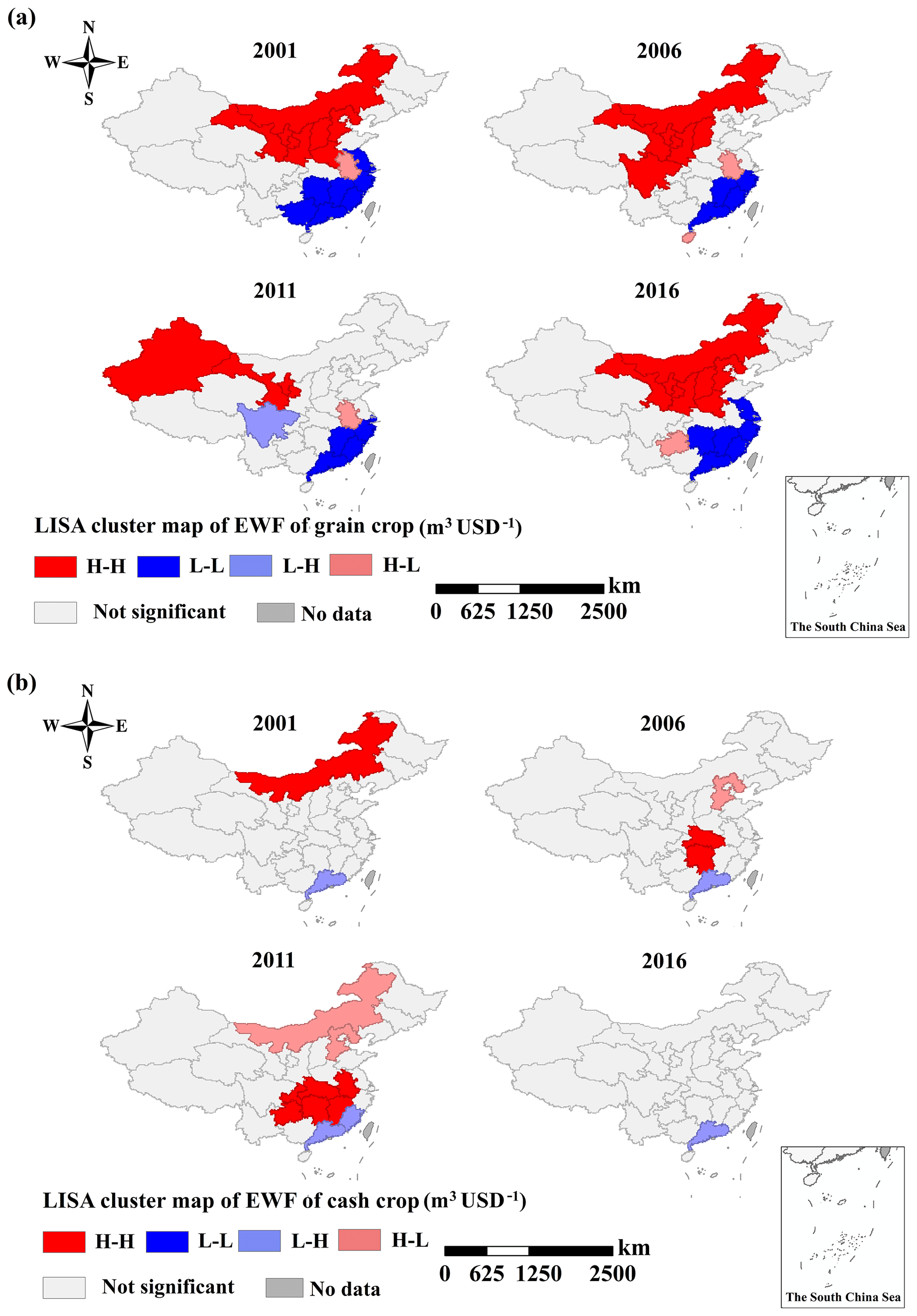
Figure 7 The LISA cluster maps of economic value-based water footprint (EWF) of (a) grain and (b) cash crops.

The LISA cluster maps of EWF of grain and cash crops are shown in Fig. 7. The H-H regions of EWF for grain crops were mainly concentrated in Ningxia, Gansu, Shaanxi, Shanxi, and Inner Mongolia, and L-L regions were mainly concentrated in Guangdong, Zhejiang, Fujian, and Jiangxi. During the research period, the EWF of grain crops showed an obvious and stable positive spatial correlation. Generally, the spatial agglomeration pattern of the EWF of grain crops was stable. As for cash crops, the LISA maps of four representative years show great changes. Only in 2011 is a certain positive spatial correlation shown, with four provinces (Hunan, Hubei, Chongqing, and Guizhou) in H-H regions. Overall, the EWF of cash crops did not show obvious spatial agglomeration. For the same crop, the spatial variations of its PWF are defined by climate and productivity. The price is one of the main factors defining the EWF. While related to the cluster maps shown in the current results for grain and cash crops, the main factor is the cultivation distribution. Regarding the grain crops, the cultivation distributions of major grain crops in China show obvious spatial agglomeration characteristics. For instance, rice is mainly distributed in central and southern China (Hubei, Hunan, Jiangxi, Guangdong, and Guangxi). Winter wheat is concentrated in the Huang–Huai–Hai Plain (Shandong, Henan, Jiangsu, Anhui, and Hebei), whereas, regarding the cash crops, the dominant crop differs among provinces (see Fig. 10b), which resulted in obvious scattered characteristics in related WFs. For example, in the north-west regions, cotton is only planted on a large scale in Xinjiang, and almost no cotton is planted in the surrounding provinces. In addition, crop prices in the main producing provinces are generally lower, while they vary depending on the regional economic level. For example, both Henan and Shandong are the main producing areas of winter wheat, but the price (0.21 USD kg⁻¹ in 2016) in Shandong, which has a more developed economy, was higher than that in Henan (0.17 USD kg⁻¹).

3.3 Synergy evaluation of PWF and EWF

Figure 8a and b show the SI between PWF and EWF of grain and cash crops across 31 provinces, respectively, over the years. Concerning grain crops, the number of provinces with negative SI were increasing. Over time, the areas with negative SI gradually expanded to the south. The SI was mostly negative in Beijing–Tianjin–Hebei, Inner Mongolia, and north-western China. In 2016, the SI of Shaanxi was −1.13, the lowest in China. The SI of Jiangxi, Chongqing, Hubei, Hunan, Jiangsu, Zhejiang, Shanghai, and other coastal areas in south-eastern China was positive. In 2016, the SI of Jiangxi was 0.62, the highest in China. Overall, the SI of grain crops was negative in Inner Mongolia and north-western China (Shaanxi, Gansu, Ningxia), whereas in Guangdong, Jiangxi, Fujian, Zhejiang, and other coastal areas in south-eastern China it was positive, with a clustered distribution. With the development of water-saving technologies and the improvement of agricultural management, China has made gratifying progress in the efficient use of water for crop production from a single physical or economic perspective. However, only by combining the physical and economic perspectives can we gain a deeper understanding of the underlying problems and catch the synergies, trade-offs, and even lose–lose relationships between reducing the water resources input for harvesting crop yields and optimizing the economic benefits per unit of water consumption in different regions.

Figure 8 Temporal and spatial evolution of synergy evaluation index (SI) of (a) grain and (b) cash crops.

As for cash crops, the SI of Tianjin, Jiangxi, and Hunan was always negative, and the lowest in China (multi-year mean values of −0.98, −0.90, and −0.74, respectively). Overall, there were more provinces with negative SI of cash crops, and the incongruity between PWF and EWF of cash crops was more significant than that of grain crops. Interestingly, the provinces with the most severe negative SI for grain crops had positive SI for cash crops. The highest SI of cash crops in 2016 occurred in Shanghai (0.39), which was lower than the SI of grain crops in the same year (0.45). At the same time, the SI of grain and cash crops in Tianjin, Tibet, and Xinjiang decreased significantly. In more provinces, the SI of grain and cash crops varied greatly and was not synchronized. For example, the SI of grain crops in Inner Mongolia and Fujian increased significantly, while the SI of cash crops showed a downward trend. Furthermore, the SI of cash crops in Shaanxi and Gansu increased significantly, while the SI of grain crops did not change significantly.

Figure 9 Production-based water footprint (PWF) vs. economic value-based water footprint (EWF) of (a) grain and (b) cash crops per province in 2016.

Taking 2016 as an example, we further look at the reasons for the lose–lose relationship between reducing the water resources input for harvesting crop yields and optimizing the economic benefits per unit of water consumption in both grain and cash crops (see Fig. 9), from the perspective of planting structure (see Fig. 10). Shaanxi province had the highest PWF in China (1.23 m³ kg⁻¹), and the second highest EWF (7.48 m³ USD⁻¹). In Shaanxi, winter wheat and spring maize with high water consumption and low yield accounted for more than 90 % of the total sown area of grain crops, with yields lower than the national averages by 24 % and 26 %, respectively. Moreover, the price of wheat in Shaanxi province (0.17 USD kg⁻¹) was lower than the national average (0.19 USD kg⁻¹). The reasons for high water consumption per unit of grain production coupled with poor economic benefits in Shaanxi province can be attributed to the above two points. In contrast, in Jiangxi province, where rice, which has low water consumption intensity, is the main grain crop (rice accounting for 95 % of the grain crops), PWF and EWF were 0.77 m³ kg⁻¹ and 3.63 m³ USD⁻¹, well below the national averages (0.93 m³ kg⁻¹, 5.04 m³ USD⁻¹).

As for cash crops, the PWF of Tianjin was 1.92 m³ kg⁻¹, the highest in China, and the EWF was 3.26 m³ USD⁻¹, the fifth highest in China, which was significantly higher than the national average (2.05 m³ USD⁻¹). It can be seen from Fig. 10b that cotton accounted for the largest proportion (70 %) in the planting structure of cash crops in Tianjin. Cotton consumed the most water per yield unit of cash crops, while the price unit of cotton in Tianjin was the second lowest in China (1.11 USD kg⁻¹), which did not reflect the advantage of cotton as a high-value crop. Jiangxi province showed the highest EWF in China (3.86 m³ USD⁻¹), and a PWF (0.96 m³ kg⁻¹) which was also higher than the national average (0.46 m³ kg⁻¹). Figure 10b shows that citrus (planting area accounting for 29 % of cash crops) and rapeseed (planting area accounting for 48 % of cash crops) are the main cash crops in Jiangxi. However, the price unit of citrus in Jiangxi was the third lowest (0.17 USD kg⁻¹, only 62 % of the national average), and the yield of rapeseed was also the third lowest (1.34 t ha⁻¹, 32 % lower than the national average). In contrast, the main cash crop in Shanxi was apple (planting area accounting for 87 % of cash crops), with low water consumption intensity and a yield which was the second highest in China (28.5 t ha⁻¹), 1.5 times larger than the national average (18.9 t ha⁻¹).

Figure 10 Planting structure of (a) grain and (b) cash crops in 31 provinces in 2016.

4 Discussion

The goal of WF regulation is to reduce its magnitude to a sustainable level (Hoekstra, 2013), but the challenges faced during implementing sustainable development are rarely encountered in a single dimension. However, previous research has most commonly adopted a single-perspective approach to WF analysis. Based on the temporal and spatial evolution of PWF and EWF, the synergy evaluation index (SI) is constructed to achieve a more comprehensive assessment in this study. This approach has led to some differences in the results of WF compared to previous research.

Table 5 Comparison between production-based water footprint (PWF) of crop production in mainland China in the current study and previous studies.

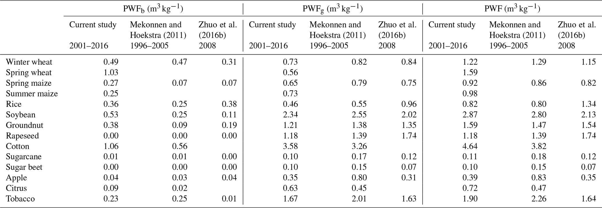
Table 6 Comparison between economic value-based water footprint (EWF) in the current results and previous studies.

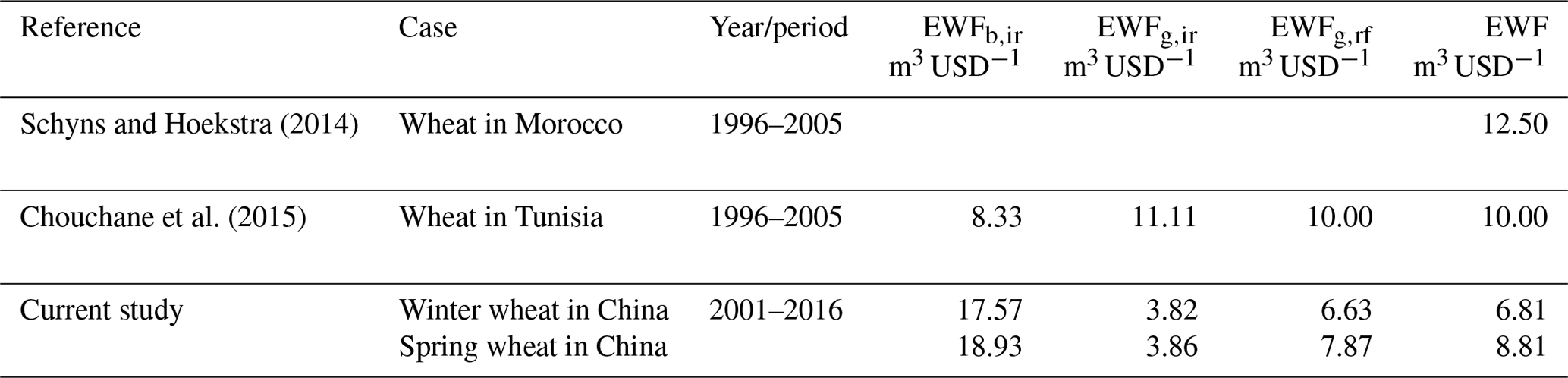
Table 5 compares the PWF results of crop production between the current study and previous ones. Differently from Mekonnen and Hoekstra (2011) and Zhuo et al. (2016b), this study distinguishes between wheat and maize varieties when calculating the WF, despite China's wheat production being mainly of winter wheat (accounting for 95 % in 2016). Due to the differences of varieties, water consumption intensity, and planting conditions, it is necessary to distinguish between crops in the provinces where spring wheat is the main crop. In addition, due to the differences in model selection and parameters, the calculation results will also be different. For example, Mekonnen and Hoekstra (2011) used the CROPWAT model and checked the crop yield at the national scale, while this study chooses the AquaCrop model and checks the crop yield at the provincial level. Both the studies of Mekonnen and Hoekstra (2011) and Zhuo et al. (2016b) were based on the 5 arcmin grid, while this research calculates the WF based on the meteorological station scale. In general, however, the crop production WF in this study is close to that of previous studies, which shows the rationality of the calculated results.

Table 6 compares the EWF of this study with previously calculated results of the economic water productivity. There were no existing EWF values for China's cases. We wish to show the available values on EWF of crops for countries other than China. Since the economic water productivity is numerically equal to the reciprocal of the EWF, the previous results are expressed in the form of EWF for comparison. The results for wheat production show that, although the average EWF is close, differences in crop varieties, planting environment, and climate conditions result in huge differences in EWF_b,ir under the same production mode. Therefore, specific problems should be investigated separately. The selection and adjustment of production modes should be made according to local conditions to promote coordinated development.

From the results of the multi-perspective analysis conducted in this study, we found that with the increase in yield and price, the PWF and EWF of crop production both showed a decreasing trend, and the EWF decreased more significantly compared with the PWF. The change of WF of cash crops was more obvious than that of grain crops. In terms of the spatial pattern, compared with cash crops, WF of grain crops had a more significant spatial correlation, and the spatial distribution of PWF was similar to that of EWF. H-H areas mainly gathered in north-western China, while L-L areas were in south-eastern coastal provinces. The average Moran's I of EWF (0.482) was higher than that of PWF (0.263).

Moreover, results show that as for grain production at the national level, the EWF_b,ir (mean 15.49 m³ USD⁻¹) was much higher than the EWF_g,ir (mean 3.11 m³ USD⁻¹), and the EWF_g,rf (mean 5.31 m³ USD⁻¹) was the closest to the average EWF in irrigation and rainfed agriculture (mean 5.41 m³ USD⁻¹). Compared with grain crops, the difference between EWF_g,ir and EWF_g,rf of cash crops was smaller, with average values of 1.90 and 2.48 m³ USD⁻¹, respectively. Moreover, the EWF of cash crops was lower than that of grain crops. It was more cost-effective to increase the input of green water than that of blue water during crop production. In north-western China, the EWF_b,ir was lower, while the EWF_g,ir and EWF_g,rf were higher; on the contrary, in southern China, the EWF_b,ir was higher, while the EWF_g,ir and EWF_g,rf were lower. Therefore, the utilization efficiency of green water resources should be improved through water retention by tillage systems and mulching. Meanwhile, more blue water can be generated through rainwater harvesting (Hoekstra, 2019). Specifically, we suggest two measures to increase the blue water efficiency in northern China. One is rainwater harvesting in the rainy season, especially for the short-term heavy rain which cannot be effectively used by crops but can easily cause soil erosion. The other one is reducing blue water consumption and loss in the field by popularizing water-saving irrigation techniques and mulching practices. Such measures are helpful to improve the utilization efficiency of both blue and green water. Based on the current results, we recommend the government to improve agricultural water use efficiency through the extension of water-saving irrigation techniques and better agricultural inputs management, especially in north-west China. High water consumption and acreages of low-economic-value crops in non-primary production areas should be reduced. For the southern regions with abundant rainwater resources, the economic benefits of irrigation are very limited; on the contrary, rainfed agriculture has obvious advantages and the potential to increase economic benefits. Therefore, farmers should improve the water conservation rate and the utilization efficiency of green water through farming systems and coverage to reduce the amount of water used for irrigation. The government should also give financial subsidies for agricultural production to those provinces where there were lose–lose relationships between reducing the water resources input for harvesting crop yields and optimizing the economic benefits per unit of water consumption. Finally, field management should be improved, especially in the utilization rate of chemical fertilizers and pesticides, to increase agricultural productivity further (Zhang et al., 2013).

There was a serious lose–lose relationship between reducing the water resources input for harvesting crop yields and optimizing the economic benefits per unit of water consumption in both grain and cash crops. In terms of grain production, the water consumption per yield was large, but the economic benefit per water consumption unit was poor in the north-west region, while the opposite was true in the south-east coastal region. Over time, the lose–lose relationship has not been alleviated, showing a relatively stable spatial pattern. Through analysis, this study shows that the unreasonable regional planting structure and crop price may be the direct cause of the incongruity between water resource consumption and economic value creation for crop production in China.

The study reveals the synergies and trade-offs of crop PWFs and EWFs. However, it is undeniable that there are some limitations and shortcomings. Firstly, in the calculation of WF, although the accuracy of the AquaCrop model in simulating crop water consumption and yield, soil field water, and fertilizer management types under different climatic conditions has been widely demonstrated, the uncertainty of results caused by the uncertainty of input parameters must be acknowledged (Zhuo et al., 2014). Secondly, this paper does not make a specific distinction between crop irrigation methods. In fact, the difference of WF results caused by different irrigation methods cannot be ignored (Wang et al., 2019). Thirdly, when calculating the WF, it is assumed that the change of crop irrigation and rainfed planting area only occurs in the data grid based on 2000, and the migration of the crop harvesting zone is not considered. Finally, this study does not focus specifically on the effects of field water and fertilizer management measures. Although there are restrictions on the availability of crop price unit data in the selection of research objects, it is still representative because the crops selected in this paper account for more than 85 % of the national crop production. As for the study perspective, this article focuses on trade-offs between water consumption and economic value creation in crop production. In fact, the ecological impacts on the environment cannot be ignored. Therefore, further research is expected to tackle this limitation by including the ecological impacts on the environment in a more comprehensive assessment. In addition, it should be noted that in the current study, the SI measures consider the spatial heterogeneities in crop WFs among provinces and the synergy levels between the current PWF and EWF. The synergy (both the PWF and EWF are lower than the national averages), trade-off (one is higher than the national average while the other is lower), or lose–lose (both are higher than the national averages) situation can be identified. The most optimized situation means high economic value generated by low water consumption. For the two provinces with high SI values, they were both in an advantageous position, while the one with a higher SI values performed better in terms of synergy between PWF and EWF. If the reference value is set by the WF benchmark (Mekonnen and Hoekstra, 2014b), then the SI will show information on efficiency. The meaning is totally different from the current one. Choosing proper reference values for different functions is highly recommended.

5 Conclusions

Based on temporal and spatial evolution analysis of WF of China's crop production from a physical and economical perspective, this study makes a comprehensive assessment by constructing a SI between PWF and EWF and reveals the synergies and trade-offs of crop water productivity and its economic value. Results show the following:

• 1.

  With the increase in yield unit and price unit, the PWF and EWF of crop production both showed a decreasing trend, and the EWF decreased more significantly. The change of WF of cash crops was more obvious than that of grain crops.

• 2.

  Compared to cash crops, WF of grain crops had a more significant spatial correlation, and the spatial distribution of PWF was similar to that of EWF. H-H areas were mainly gathered in north-western China, while L-L areas were in south-east coastal provinces. The average Moran's I of EWF (0.482) was higher than that of PWF (0.263).

• 3.

  The economic benefits of blue water and green water differed greatly, and the difference showed to be more significant for grain crops than for cash crops. Moreover, the EWF of cash crops was lower than that of grain crops. It was found to be more cost-effective to increase the input of green water than that of blue water during crop production.

• 4.

  In terms of grain production, the water consumption per yield unit was large but the economic benefit per water consumption unit was poor in the north-west region, while the opposite was true in the south-east coastal region. The trade-offs have not been alleviated over time, showing a relatively stable spatial pattern. These findings show that the unreasonable regional planting structure and crop price may be the direct cause of the lose–lose relationships between water resource consumption and economic value creation for crop production, so this issue should be tackled by coordinated governmental action, to balance the economic benefits of the water-intensive crops in different regions.