the Creative Commons Attribution 4.0 License.
the Creative Commons Attribution 4.0 License.
 | 31 Mar 2021
Improving soil moisture prediction of a high-resolution land surface model by parameterising pedotransfer functions through assimilation of SMAP satellite data
Ewan Pinnington
Javier Amezcua
Elizabeth Cooper
Simon Dadson
Rich Ellis
Jian Peng
Emma Robinson
Ross Morrison
Simon Osborne
Tristan Quaife
Pedotransfer functions are used to relate gridded databases of soil texture information to the soil hydraulic and thermal parameters of land surface models. The parameters within these pedotransfer functions are uncertain and calibrated through analyses of point soil samples. How these calibrations relate to the soil parameters at the spatial scale of modern land surface models is unclear because gridded databases of soil texture represent an area average. We present a novel approach for calibrating such pedotransfer functions to improve land surface model soil moisture prediction by using observations from the Soil Moisture Active Passive (SMAP) satellite mission within a data assimilation framework. Unlike traditional calibration procedures, data assimilation always takes into account the relative uncertainties given to both model and observed estimates to find a maximum likelihood estimate. After performing the calibration procedure, we find improved estimates of soil moisture and heat flux for the Joint UK Land Environment Simulator (JULES) land surface model (run at a 1 km resolution) when compared to estimates from a cosmic-ray soil moisture monitoring network (COSMOS-UK) and three flux tower sites. The spatial resolution of the COSMOS probes is much more representative of the 1 km model grid than traditional point-based soil moisture sensors. For 11 cosmic-ray neutron soil moisture probes located across the modelled domain, we find an average 22 % reduction in root mean squared error, a 16 % reduction in unbiased root mean squared error and a 16 % increase in correlation after using data assimilation techniques to retrieve new pedotransfer function parameters.
- Article
(13028 KB) - Full-text XML
-
Supplement
(378 KB) - BibTeX
- EndNote


Land surface models are important tools for translating meteorological forecasts and reanalyses into real-world impacts by providing schemes for how energy, water and other matter will interact with the Earth's surface, outputting relevant diagnostics and variables and understanding the role of variability in the terrestrial hydrological cycle in the Earth system. As the spatial resolution of available meteorological information has become increasingly fine (Clark et al., 2016), it is necessary to ensure land surface models can utilise this information at its native resolution in order to provide outputs that are as accurate as possible for local populations. In this paper, our focus is on soil moisture, which plays an essential role in agriculture (Asfaw et al., 2018), weather and climate prediction (Hauser et al., 2017) and land surface energy partitioning (Beljaars et al., 1996; Bateni and Entekhabi, 2012). The modelling of soil moisture is highly sensitive to driving precipitation and model parameterisations (Pitman et al., 1999). Typically, models of soil moisture will determine parameters based on spatial datasets of soil texture information using pedotransfer functions such as those defined by Cosby et al. (1984) for the Brooks and Corey (1964) soil model. The majority of pedotransfer relationships are calibrated for point samples of soil for a specific geographic location (Cosby et al., 1984; Wösten et al., 1999; Schaap et al., 2004; Tóth et al., 2015). Selecting the appropriate set of pedotransfer functions for the modelled area will allow for more representative results. It is unclear how these calibrations of pedotransfer functions and their resulting soil model parameters relate to the varying spatial scales of modern land surface models, and indeed the use of additional streams of information from remote sensing and in situ observations is seen as increasingly important for calibration and validation (Van Looy et al., 2017). Pedotransfer functions can be continuous or discrete (setting predefined model parameters for different ranges of soil texture). Discrete examples of pedotransfer functions can be found in Wösten et al. (1999) for the van Genuchten (1980) soil model. Continuous versions of these functions may be preferential as they provide greater heterogeneity for resulting soil model parameter maps, which may be more realistic. Tóth et al. (2015) provide more recent examples of continuous pedotransfer functions for the van Genuchten (1980) model. For this paper, continuous functions will also allow us to seek updated parameter values that improve the prediction of a land surface model at a given spatial scale and properly account for uncertainty in both the soil's information and resulting model predictions.
There now exists a large amount of information from different satellite missions relating to the spatial and temporal variability of soil moisture. These can be based on either active (e.g. the Advanced Scatterometer (ASCAT); Wagner et al., 2013) or passive (e.g. the Soil Moisture Ocean Salinity (SMOS) mission; Kerr et al., 2001) observing instruments with good results found when combining both (e.g. the Soil Moisture Active Passive (SMAP) mission; Entekhabi et al., 2010). The NASA SMAP mission was originally designed with both an active and passive sensor on board; soon after launch in January 2015 the active sensor malfunctioned. Sentinel 1 is now used as the active component in the SMAP soil moisture retrieval. Recent validation studies have shown SMAP to perform well in comparison with other satellite estimates (Montzka et al., 2017; Chen et al., 2018; Peng et al., 2021). These remotely sensed products are available at scales comparable to current land surface models from 50 km down to 9 km. Traditional in situ observations of soil moisture are made at a single point using a variety of different methods (Walker et al., 2004). These in situ measurements provide accurate estimates of the true state of the amount of water contained within the soil. However, the scale of such measurements can be unrepresentative of the scales of the model, even when land surface models are run at a high resolution (∼ 1 km). The recent development of cosmic-ray neutron sensing soil moisture probes (Zreda et al., 2008) somewhat alleviates this issue. Cosmic-ray neutron probe observations have a variable spatial footprint dependent on atmospheric air density (130–240 m; Köhli et al., 2015; with some studies quoting a diameter of ∼ 600 m; Desilets and Zreda, 2013) that is much more representative of land surface model estimates than that of traditional soil moisture probes. There are now good networks of cosmic-ray probes within several countries (Zreda et al., 2012). This is true in the UK where the COsmic-ray Soil Moisture Observing System United Kingdom (COSMOS-UK) network (Evans et al., 2016) has been established by the UK Centre for Ecology and Hydrology (UKCEH); it has been returning observations since 2013 (Stanley et al., 2019). These observations can act as valuable validation data of both satellite and land surface model soil moisture estimates (Duygu and Akyürek, 2019).
Data assimilation provides methods for combining new observations with land surface models in order to improve predictions. These techniques can either be used for state-estimation to update soil moisture values of the model in real time as new observations are available (Liu et al., 2011; Draper et al., 2012; De Lannoy and Reichle, 2016; Kolassa et al., 2017) or for model parameter estimation to find improved calibrations which better represent the observations (Rasmy et al., 2011; Sawada and Koike, 2014; Yang et al., 2016; Pinnington et al., 2018). Unlike traditional calibration procedures, data assimilation and other associated Bayesian optimisation methods always take into account the relative uncertainties given to both model and observed estimates to find a maximum a posteriori estimate (Beven and Binley, 1992; Thiemann et al., 2001; Vrugt et al., 2003; Moradkhani et al., 2005; Nearing et al., 2010; Mizukami et al., 2017). Previous studies have used data assimilation to update the soil parameters of land surface models (Rasmy et al., 2011; Sawada and Koike, 2014; Yang et al., 2016; Han et al., 2014). However, we are unaware of any studies using data assimilation to update the parameters of pedotransfer functions to improve land surface model predictions. Updating the parameters of these pedotransfer functions by combining them with observations from satellites addresses a key uncertainty within their calibration with respect to land surface models, adding additional information about spatial heterogeneity and the larger scales of both satellite and land surface model estimates. Many previous studies optimising model soil parameters have taken a filtering data assimilation (DA) approach (Moradkhani et al., 2005; Montzka et al., 2011; Han et al., 2014; Baatz et al., 2017; Botto et al., 2018), leading to the recovery of a time series of parameter values as additional data is assimilated through time. In this study we use a smoother method, i.e. one that uses all observations in the spatial domain within a time window of a given length. Then, the static parameters are obtained by a single minimisation process (which can contain iterative steps). Smoothers can be used in a sequence of “analysis windows” (as it is done in operational numerical weather prediction), but in this study we only use one of these windows since the parameters we are searching for do not vary in time.
We have used the Land Variational Ensemble Data Assimilation Framework (LAVENDAR) (Pinnington et al., 2020) to combine soil moisture estimates from the NASA SMAP mission with the Joint UK Land Environment Simulator (JULES) model run at a high resolution (1 km) and update the parameters of the Tóth et al. (2015) pedotransfer functions for the van Genuchten (1980) soil model. In our experiments, we assimilated 2016 SMAP data and then ran a hindcast for the year 2017. The experiments were conducted over a subdomain of the UK due to considerations of computational expense. We selected the region of East Anglia due to it being equally susceptible to flooding and drought and therefore displaying a good dynamic range of soil moisture values. This region also had a good availability of high-quality SMAP data (here we use Level-3 SMAP soil moisture observations) and a high distribution of COSMOS probes to allow for thorough validation of any results. While reducing the spatial domain in our experiments eased the computational load, we were still modelling over 30 000 grid points due to the high resolution of the domain.
We defined two objectives for this study: firstly, to examine the ability of 9 km SMAP data to update pedotransfer parameters in a 1 km land surface model and, secondly, to assess the resulting prediction of modelled soil moisture against (a) SMAP data from a different time period and (b) independent in situ data from the COSMOS-UK network. We also assess the impact on modelled latent and sensible heat flux at three flux tower sites.
2.1 JULES land surface model
Joint UK Land Environment Simulator (JULES) is a community developed process-based land surface model and forms the land surface component in the next-generation UK Earth System Model (UKESM). A description of the energy and water fluxes is given in Best et al. (2011), with carbon fluxes and vegetation dynamics described in Clark et al. (2011). We drive the JULES model with the Climate Hydrology and Ecology research Support System meteorology (CHESS) dataset (Robinson et al., 2017), which is a 1 km daily dataset of meteorological variables; an example implementation of JULES with the CHESS-met dataset can be found in Martínez-de la Torre et al. (2019). In our experiments, we have used JULES version 5.3; the code and model settings are available through the Met Office JULES repository (https://code.metoffice.gov.uk/trac/jules, last access: 29 March 2021), with Rose suite number u-bq357. This model setup is based on the Rose suite u-au394 used to create the CHESS-land dataset (Martinez-de la Torre et al., 2018). The JULES model utilises the Harmonised World Soil Database (HWSD) (Fischer et al., 2008) as the underlying soil texture map for the creation of its soil parameter ancillaries using a pedotransfer function (see Fig. 1). The HWSD has been gap-filled in urban areas where no information is available as we ran JULES without urban tiles switched on. The soil scheme is made up of four separate layers with depths of 0.1, 0.25, 0.65 and 2 m respectively. We have chosen to keep JULES in its default soil-layer setup so that our optimised parameters are relevant to the wider JULES modelling community. This is despite the fact that SMAP satellite observations are typically sensitive to the top ∼5 cm of soil (Entekhabi et al., 2010), with some studies suggesting L-band radiometer measurements may only be sensitive to the top ∼2.5 cm (Zheng et al., 2019). This could introduce an additional source of error into our DA system. To ensure that the effect of this is not too great, we show that there is only a small difference in soil moisture between depths of 10 and 5 cm in the JULES model in the Supplement (Fig. S1). We have also rerun the entire data assimilation experiment with a 5 cm topsoil layer in JULES and show that the recovered parameter distributions are similar to those recovered with a 10 cm topsoil layer in Figs. S2 and S3. It is necessary to find an appropriate initial state before running a land surface model such as JULES, and it has been shown that, without a suitable spin-up period, forecast skill can be impacted (Maurer and Lettenmaier, 2002). We include a 4 year spin-up period at the start of each JULES run to allow the soil moisture state to reach a point of equilibrium after parameter values are changed. For the JULES spin-up, the model is run from an initial value (defined by the saturated soil moisture model parameter) over the same year of forcing data, here 2015, to reach an equilibrium soil moisture state for any given set of soil hydraulic parameters. We show this model spin-up for three unique soil parameter sets at the same location in Fig. S4.

Figure 1Maps of soil properties from the Harmonised World Soil Database (HWSD) (Fischer et al., 2008) used in the creation of the JULES soil parameter ancillaries with the Tóth et al. (2015) pedotransfer functions. Blue dots show locations of COSMOS-UK probes, crosses show flux tower locations and the black dot shows the location of London, UK.
2.2 Pedotransfer functions
The JULES model implements both the Brooks and Corey (1964) and the van Genuchten (1980) models of soil physics, with the model of choice being selected by a switch in the JULES namelist files. The JULES implementation of these models can be found in Clark et al. (2011). In this paper we have used the van Genuchten (1980) soil parameterisation scheme and have selected a set of pedotransfer functions from Tóth et al. (2015). The Tóth et al. (2015) pedotransfer functions have been calibrated across a large range of European soils and should be representative of the study area. The mathematical formulation of these pedotransfer functions is
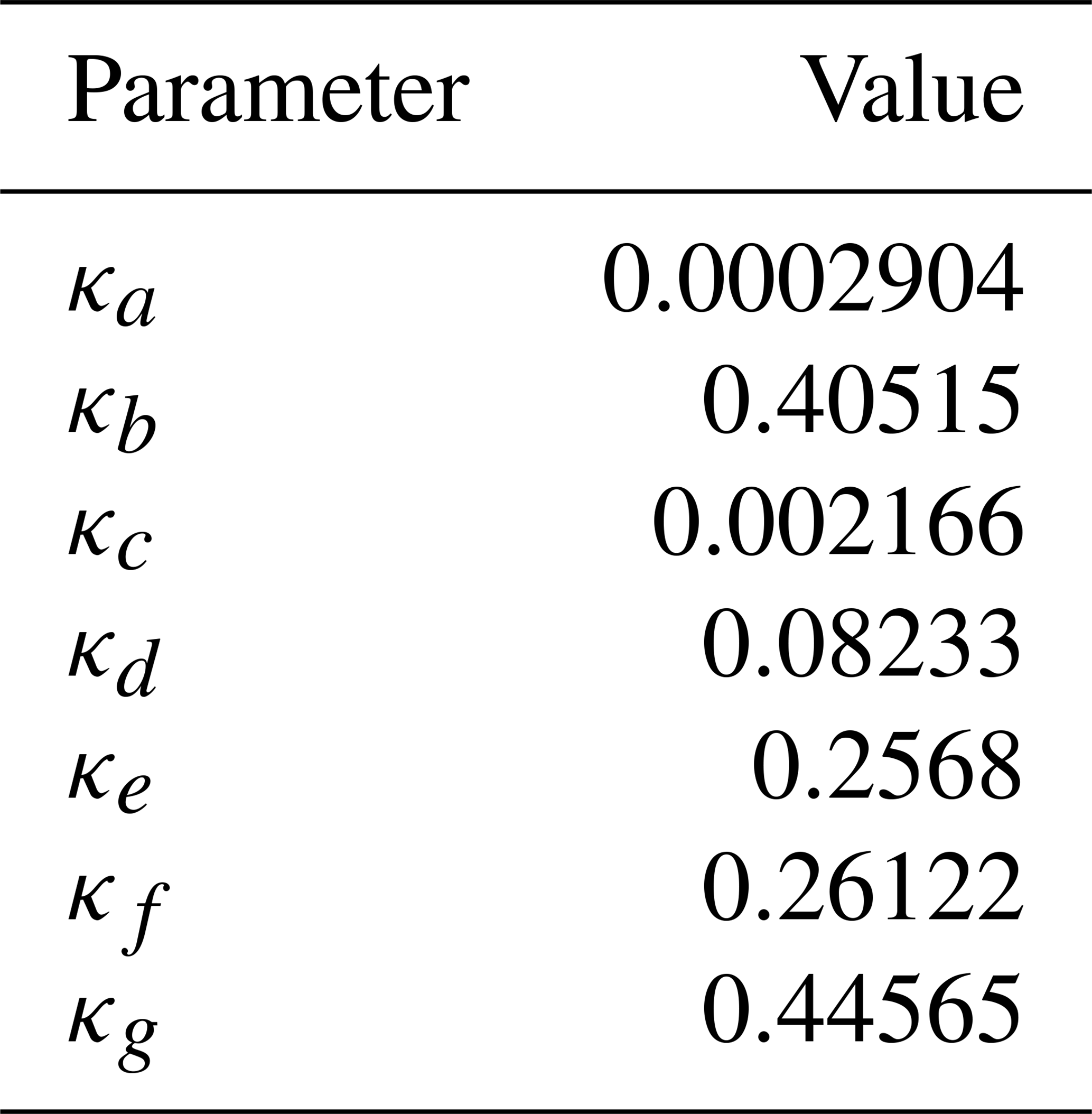
where θres is the residual soil moisture (m3 m−3), θsat is the saturated soil moisture (m3 m−3), α and (N−1) are parameters of the van Genuchten (1980) soil model (–), Ksat is the saturated hydraulic conductivity (kg m−2 s−1), are model parameters to be optimised (values given in Table 1) and are static model parameters (values given in Table 2). We optimise the parameters controlling the impact of the bulk density ρ (g cm−3), fraction of clay and silt (fclay, fsilt) ( %) and the cation exchange capacity (CEC) (mEq 100 g−1) as these terms have a first-order impact on the outputted van Genuchten (1980) soil parameters. The organic carbon content (Corganic) (%), soil pH value and topsoil flag have a less pronounced effect on the van Genuchten (1980) soil parameters. We treat the top two soil layers of JULES as topsoil (topsoil=1) and the bottom two as subsoil (topsoil=0). From Eq. (1) we can see that defining a soil as topsoil will act to increase the saturated hydraulic conductivity and the value of α, which will both allow water to flow more freely through the soil. The prior values for the parameters are shown in Table 1. We used the values given by Tóth et al. (2015) for the prior except for ϕo for which we found better results (experiments not shown) when the magnitude of this parameter was increased. To create the JULES soil parameter ancillary files, these pedotransfer functions are applied to soil texture information from the HWSD (Fischer et al., 2008) at a 1 km resolution. The DA system used here optimises values for the parameters in Table 1 across the whole domain rather than on a grid-by-grid basis. In this way, the varied soil properties across the domain give us a form of orthogonal constraint within the assimilation and allow us to recover a single set of pedotransfer functions that are valid in space and time.
Table 1Prior values for parameters of the Tóth et al. (2015) pedotransfer functions used in experiments.
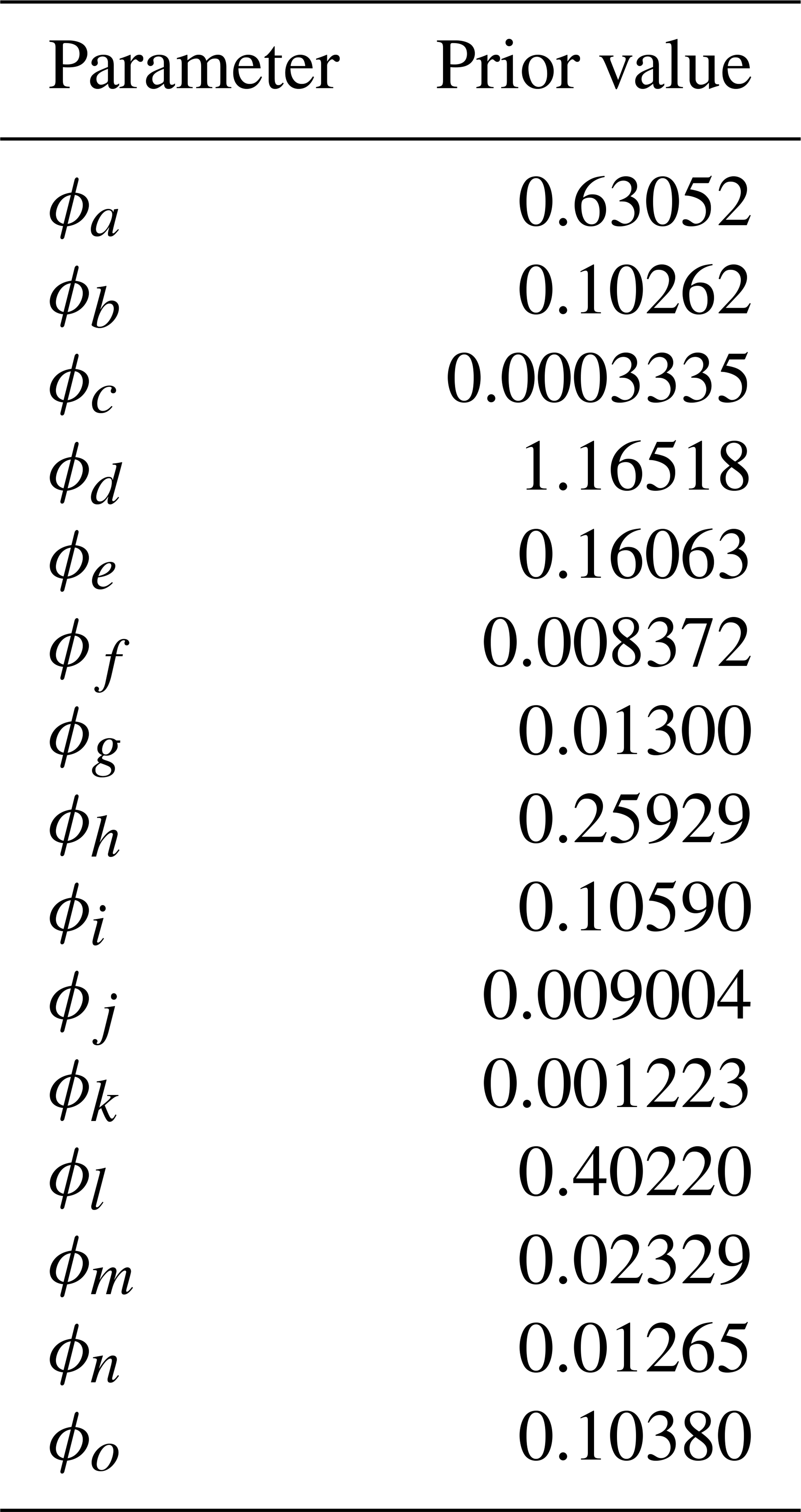
Table 2Static parameter values for the Tóth et al. (2015) pedotransfer functions used in experiments.
2.3 SMAP observations
The NASA Soil Moisture Active Passive (SMAP) satellite mission provides estimates of soil moisture every 2–3 d (Entekhabi et al., 2010). The mission is an orbiting observatory with a passive radiometer and an active radar instrument. SMAP was designed to deliver a 36 km spatial resolution estimate of soil moisture from the passive instrument alongside a 9 km estimate from a retrieval using both the passive and active sensors. After its launch in January 2015, the radar instrument malfunctioned. Subsequently ESA's Sentinel 1 mission was used as a replacement for the active sensor. For the work in this paper we use the 9 km Level-3 soil moisture product (version 3); this product has a relatively low bias (Colliander et al., 2017; Zhang et al., 2019). However, it has been shown there is a wet bias present in the Level-4 SMAP product (Reichle et al., 2017). As part of the retrieval procedure, SMAP relies on some ancillary information; one example of this is soil texture for which the Harmonised World Soil Database (HWSD) (Fischer et al., 2008) is used to calculate the soil dielectric constant for use within the retrieval algorithm. The use of such ancillary data in the retrieval could introduce additional biases into the SMAP soil moisture estimates that are not consistent with estimates from the land surface model we are comparing to. However, as the HWSD is also used to create the JULES soil parameter ancillary files, this effect should be minimised. We prescribe an error of 0.05 m3 m−3 for SMAP observations in the assimilation algorithm. Although the SMAP baseline aim for error is 0.04 m3 m−3, other studies have found slightly higher values for the error in Level-3 SMAP observations (0.043 m3 m−3, Colliander et al., 2017; 0.057 m3 m−3, Li et al., 2018; and 0.054 m3 m−3, Zhang et al., 2019); we therefore chose a value between these studies. We have only used SMAP observations corresponding to the best retrieval quality flag and surface flag in experiments. The effect that removing poor-quality observations has on the total number of observations assimilated can be seen in Fig. 2. The experiment area of the east of England is predominantly flat arable land, which should allow for good-quality SMAP retrievals; there are also coastal and urban areas where SMAP retrievals will be unreliable. This area is also prone to cloud cover, which could cause gaps in the SMAP observational record.
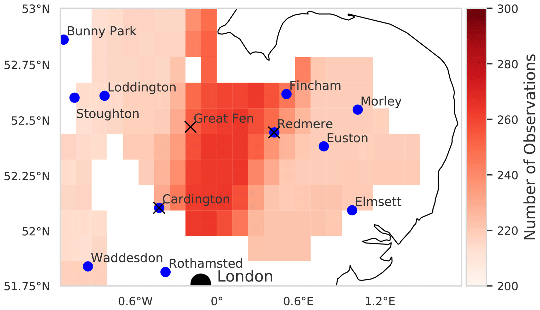
Figure 2Location of COSMOS probes (blue circles) and flux towers (black crosses) used in validation. Red shading indicates number of SMAP observations assimilated in experiment period (2016). No colour corresponds to no observations being assimilated in that location due to low-quality retrieval or surface flag. The black dot shows the location of London, UK.
2.4 COSMOS-UK observations
The COSMOS-UK network has been producing observations of soil moisture and other meteorological variables at an expanding number of stations (currently 52) since 2013 (Stanley et al., 2019). For the area of interest in this paper, we have 11 stations available to us with data for the relevant time period (see Fig. 2). Some of these stations may not be representative of JULES model estimates due to the current setup of JULES not considering some processes (groundwater, organic soils, urban tiles). Cosmic-ray sensing soil moisture probes have a variable depth as well as horizontal sensitivity (Zreda et al., 2008). There are many studies translating the cosmic-ray neutron intensity measured at COSMOS probe sites to soil moisture (Baatz et al., 2014; Bogena et al., 2015; Köhli et al., 2015). There have also been efforts to relate modelled soil moisture to cosmic-ray neutron intensity, such as the COsmic-ray Soil Moisture Interaction Code (COSMIC) (Shuttleworth et al., 2013; Rosolem et al., 2014). The COSMOS-UK network uses the N0 method described by Baatz et al. (2014) to diagnose values for the soil moisture and then the method of Köhli et al. (2015) to calculate the representative depth for each COSMOS probe measurement. The COSMOS sites in our experiment domain have a representative depth of between 14 and 40 cm dependent on conditions when measurements are made. To make a fair comparison between the COSMOS-UK and JULES soil moisture estimates, we have constructed a simple variable depth algorithm for JULES which takes a weighted average of the different soil layers of the model given the relative depth of the COSMOS-UK observation. This is defined as
where θD is the JULES modelled soil moisture at the COSMOS-UK representative depth (D), and θ10, θ25 and θ65 are the top, second and third layer soil moisture estimates from the JULES model.
2.5 Flux tower observations
In order to understand how updating the JULES soil parameters of the model might effect the model prediction of latent and sensible heat flux, we compare prior and posterior estimates to observations at three flux towers. The location of these flux towers is shown by black crosses in Fig. 2; two of these flux towers are located near to COSMOS-UK sites (Cardington and Redmere), and so the black cross is displayed over the blue dot signifying the COSMOS-UK location.
The Met Office site at Cardington (29 m above sea level) is a 18 ha area laid mainly to manicured grass set within generally flat, semi-rural surroundings (Osborne and Weedon, 2021). The site has been making continuous subsoil, surface and near-surface measurements since 1996. The turbulence fluxes we use here were calculated over 30 min intervals based on the eddy-covariance technique using tower data at 10 m height. For latent heat fluxes, the Licor LI-7500 high-frequency open-path gas analyser was used for water vapour as well as the vertical wind component from a Gill HS-50 3-D sonic anemometer. The same anemometer was used to monitor the rapid response in both the virtual temperature and vertical wind required for the sensible heat flux.
The Redmere and Great Fen sites are located on lowland peat soils in the East Anglian Fens. Both sites are nodes of the UK Land Flux Network (UKLFN) operated by the UK Centre for Ecology and Hydrology (UKCEH). The Redmere site is cropland, producing maize and lettuce in 2016 and 2017, respectively. The Great Fen site is an area of extensively managed grassland. Instrumentation is identical at both locations, consisting of a Windmaster ultrasonic anemometer (Gill Instruments Ltd.) and a LI-7500A infrared gas analyser (LI-COR Biosciences, Ltd). Raw (20 Hz) EC (eddy covariance) data were reduced to 30 min flux densities using the EddyPRO v7.0.6 flux calculation software (Fratini and Mauder, 2014). Data quality control included outlier removal and filtering using site-specific friction velocity (u*) thresholds (Papale et al., 2006; Reichstein et al., 2005). Gaps in the EC data were filled using the marginal distribution sampling approach (Reichstein et al., 2005, 2014). The Redmere and Great Fen dataset and full details of the sites and flux methodology are available in Morrison et al. (2020).
2.6 Data assimilation framework
In order to estimate the identified pedotransfer function parameters, we use the LAVENDAR data assimilation framework (Pinnington et al., 2020). This framework utilises a hybrid DA technique similar to that of the iterative ensemble Kalman smoother (IEnKS) (Bocquet and Sakov, 2013). A smoother is different than a filter (e.g. the ensemble Kalman filter Evensen, 2003), in that it uses batches of observations which are taken over a time window of given length and the whole spatial domain, as opposed to just in a time instant. These observations are combined with the model evolution over this window, and a minimisation process is performed to obtain initial conditions for the state–parameter values. It is possible to run a sequence of smoother steps for successive windows, but our study only uses a 1-year-long assimilation window as the parameters we are optimising do not vary in time.
Using a smoother instead of a filter has advantages (Lorenc and Rawlins, 2005) in that (a) more observations can be used to constrain the problem solution and (b) information from the model evolution is implicitly used in the search process. However, using a smoother requires computing the Jacobian of the model, the so-called tangent linear model (TLM) and the related adjoint model (AM), the TLM–AM (Courtier et al., 1994). Computing and maintaining the TLM–AM is not a trivial task, and in fact we do not have this for JULES. The IEnKS solves this problem by replacing the role of the TLM–AM by four-dimensional covariances, i.e. covariances defined over time and space. These covariances are computed as sample estimators of a given ensemble. The iterative nature of the method means that it finds the solution to the minimisation problems using inner iterations rather than a single step (hence the variational nature), and this helps when the distributions of the variables/parameters of interest are not Gaussian. We provide details of the method in Appendix A. Furthermore, to understand the variants of the ensemble Kalman smoother and its position within the hybrid DA methods, the reader is referred to Evensen (2018).
We show a schematic of how this system works in Fig. 3; this involves running an ensemble of JULES models, with each model in the ensemble utilising a distinct soil ancillary dataset. Each ensemble member's ancillary file is created by sampling from the normal distribution defined by mean xb and variance (0.1×xb)2), where , with ϕa, …, ϕo taking the values given in Table 1, then using each unique set of sampled parameters within Eq. (1) applied to the HWSD maps of soil properties (see Fig. 1) for the whole domain. Although van Genuchten and hydraulic conductivity parameters can be described by logarithmic distributions, it is less clear what distribution is best for the pedotransfer function (PTF) parameters optimised here. We therefore made the naive assumption of a normal distribution in the first instance as this gave us good results. In this type of experiment, the number of ensemble members will control the quality of the results, with a larger ensemble more likely to identify the optimum parameters. However, running a land surface model at a 1 km spatial resolution over the specified domain is computationally expensive; we therefore use an ensemble size of 50 in our experiments. In order to compare the 1 km estimates of soil moisture from JULES to the 9 km SMAP estimates, we create an observation operator which aggregates the JULES grid cells within each SMAP pixel by taking a spatial average of all JULES estimates which fall in the bounds of the SMAP grid cell. There is no need to project increments from the spatially averaged 9 km model estimates back to the 1 km model grid as the assimilation is only optimising the 15 PTF parameters for the whole domain and the update to soil moisture will be implicit. The aggregated spatial observation operator will introduce an additional source of representativity error alongside the observational error of SMAP and the inherent model error within JULES. It has been shown that, for variational methods such as the one used in this paper, these additional sources of error (model error, representativity error, etc.) can be included in the observational term of the cost function by inflating the diagonal observation error variance (Howes et al., 2017). Although observation error inflation is rare in relation to filtering DA methods, it is commonly used with variational methods and smoothers, especially in numerical weather prediction (Hilton et al., 2009; Bormann et al., 2015; Minamide and Zhang, 2017; Fowler et al., 2018; Wang et al., 2019). Observation error inflation is required due to the fact that all observations are used at once in the assimilation, whereby we minimise a cost function containing a prior term and an observational term. The greater the number of observations in the observational cost function term, the higher the weight they have in the optimisation. This can lead to the prior term being completely negated and hence the retrieval of non-physical parameters. Observation error inflation would not be required if the correct specification for the observation error correlations (in space and time), model error and representativity error were included. These, however, are hard to diagnose, and it has been shown that in the absence of such information, observation error inflation is required for an optimal DA system (Stewart et al., 2014). For this reason, and due to the large number of observations assimilated in our 1-year assimilation window (28 698), we inflate the specified observational error by a factor of 4. If a filtering DA system were being used, utilising a bias aware method such as that presented by Ridler et al. (2017) could help represent some of the additional sources of error discussed here.
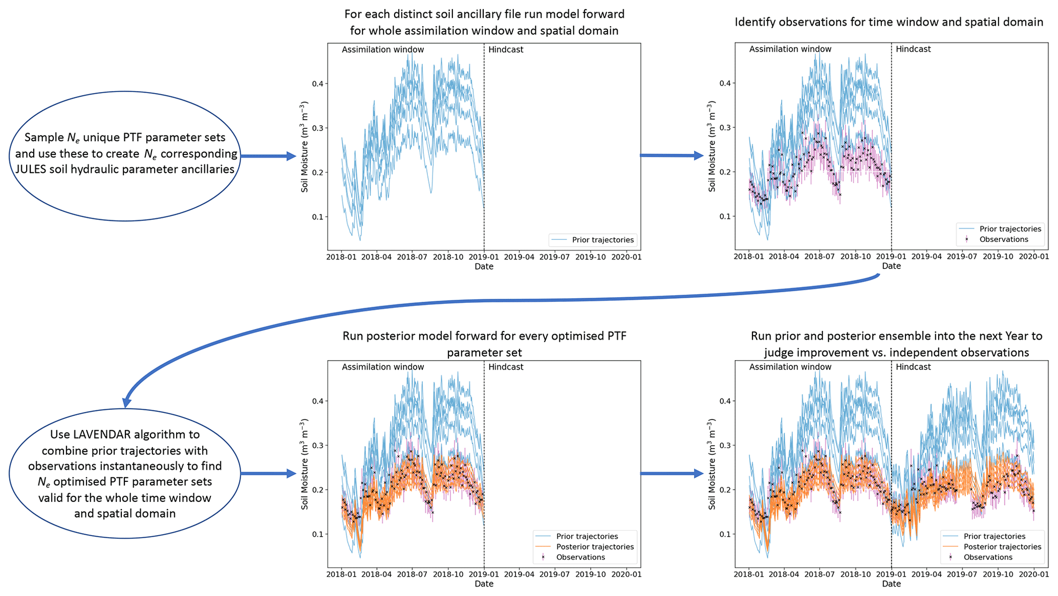
Figure 3Schematic of the LAVENDAR data assimilation framework, showing the workflow for the experiment. Here Ne is the chosen size of ensemble; in the schematic we show Ne=5, but in practice for our experiments Ne=50.
2.7 Experiment formulation
We conducted our pedotransfer function parameter estimation for the year of 2016 using all SMAP observations in this period. We also ran the prior and posterior JULES ensembles into 2017 so that we could judge the results against independent SMAP observations in a “hindcast” experiment, allowing us to judge if any skill added by the assimilation persisted into the future. For the 2016–2017 period, we then used the available COSMOS probe observations for validation, comparing both prior and posterior JULES soil moisture estimates to these observations. Using the COSMOS-UK observations in this way gives us a better understanding of whether information added by the assimilation of SMAP observations can help to improve model estimates at in situ scales.
3.1 Assimilation output
The input to the data assimilation routine is an ensemble of 50 unique Tóth et al. (2015) PTF parameter sets drawn from a prior distribution (representing our best a priori guess of the true PTF parameters), the corresponding JULES runs (2016–2017) for each PTF parameter set and all the SMAP observations for the year 2016 over the experiment domain. The output of the data assimilation is an ensemble of 50 optimised (posterior) PTF parameter sets, valid for the whole experiment domain and time; this allows us to calculate the posterior JULES soil ancillary files for each optimised parameter set and the corresponding posterior JULES model runs for 2016–2017. Figure 4 shows the prior and posterior parameter distributions for the 15 optimised parameters of the Tóth et al. (2015) pedotransfer functions. Prior distributions for the 50 JULES ensemble members are shown in light grey, with posterior distributions shown as dark grey. We can see that while the DA procedure made large updates to some parameters compared to their prior values, others have not changed, with their mean appearing to be in a very similar place. One of the parameters with a strong change is ϕa, which is decreased compared to the prior; this parameter controls the absolute magnitude of the saturated soil moisture (θsat). Decreasing it will reduce the absolute saturated soil moisture and allow the soil texture information to have more impact on the diagnosed van Genuchten (1980) model parameter. This can be seen in Fig. 5, where we show the updated PTF parameters' effect on the mean estimate of the JULES model soil parameters when applied to the spatial maps of soil properties from the HWSD. We can see how different areas of distinct soil texture (see Fig. 1) behave differently based on the PTF parameter updates after DA. For some parameters, we see the majority of grid cell parameter values increase or decrease, θsat and respectively, whereas for and θcrit, we see an increase or decrease in grid cell parameter values dependent on the underlying soil properties (sandier soils lead to an increase; less sand and more clay correspond to a decrease).
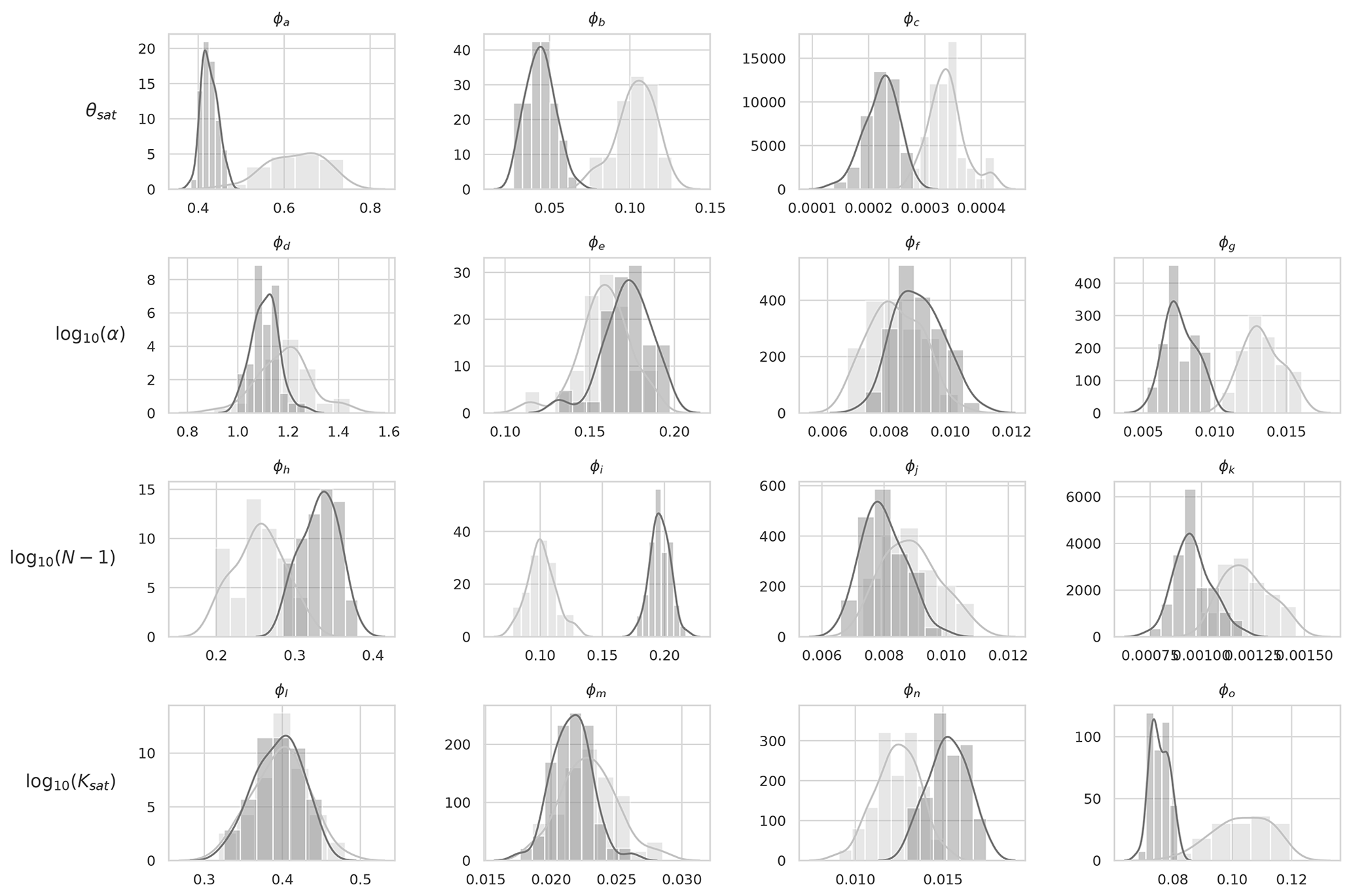
Figure 4Distributions of prior and posterior pedotransfer function parameters grouped by the term in the equations (Eq. 1) that they relate to (see row labels). Light grey: parameter distribution for the prior ensemble; dark grey: parameter distribution for the posterior ensemble.
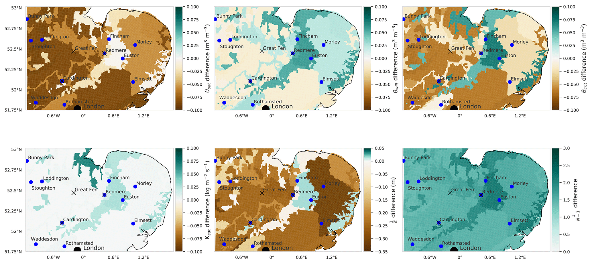
Figure 5Maps showing the difference between the prior and posterior mean JULES model soil parameters, created by applying the prior and posterior PTFs to the HWSD maps of soil properties. Brown corresponds to a decrease in the soil parameter after data assimilation and green to an increase.
In Fig. 6, we show the difference between mean water budget variable estimates (soil moisture, evapotranspiration and runoff) in 2016 for the prior and posterior JULES model ensemble. The grid cells that are darker blue correspond to the posterior ensemble estimate being higher after assimilation, and grid cells that are darker red correspond to the posterior estimate being lower. We can see that after calibration of the pedotransfer function parameters, the domain has not had a uniform increment to the value of mean soil moisture, evapotranspiration or runoff. This is due to the fact that soil-texture-specific parameters have been optimised, allowing the different distinct areas of soil type defined by the HWSD (see Fig. 1) to behave differently rather than having a uniform correction across the modelled area. Across the whole domain, we find an average increase of 0.03 m3 m−3 in mean soil moisture estimates after data assimilation. We can see that in order to update PTF parameter values to find soil moisture estimates that more closely match the SMAP observations, both evapotranspiration and runoff model estimates have also been modified. In areas of sandy soils, wetter soil moisture values have been achieved by a decrease in evapotranspiration offsetting a slight increase in runoff. In areas of high clay content, wetter soil moisture values have been achieved by a larger decrease in runoff compared to an increase in evapotranspiration. For silty soils, we find a drier value of soil moisture for the posterior compared to the prior, with a less prominent impact on evapotranspiration and runoff. Figure 6 also allows us to see the high resolution of the JULES model when run with the CHESS data; for this domain we have over 30 000 individual model grid cells.
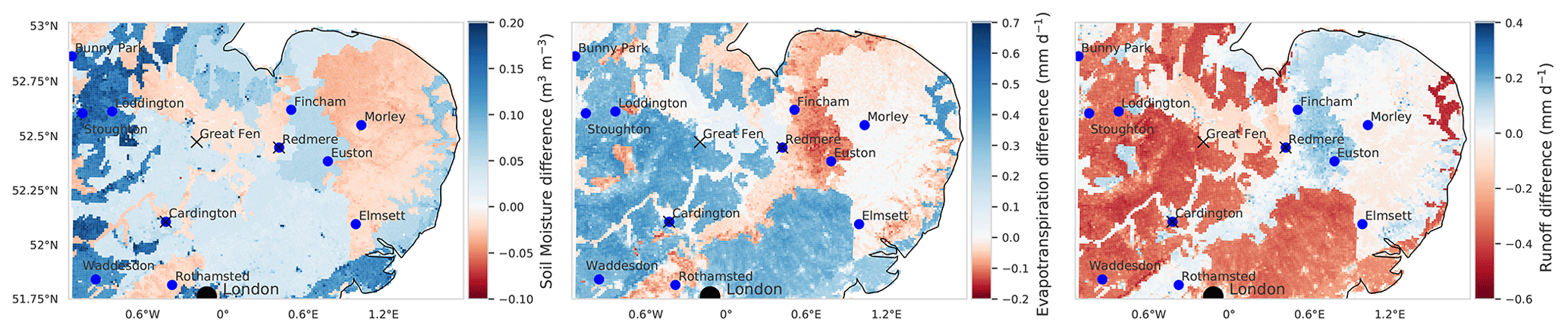
Figure 6Map showing the difference between yearly mean soil moisture for the prior and posterior ensemble of JULES model runs in 2016. Blue corresponds to the posterior ensemble estimate being wetter, and red corresponds to the posterior being drier.
Figure 7 shows the error reduction after performing data assimilation when comparing JULES spatially aggregated estimates to SMAP observations. This is computed as , where RMSEprior is the JULES prior ensemble mean root mean square error (RMSE) when compared to 2016 SMAP observations, and RMSEpost is the JULES posterior ensemble mean RMSE when compared to 2016 SMAP observations. As we are minimising a cost function to find optimised values of PTF parameters valid for the whole spatial and temporal domain, it is possible the optimisation may have to degrade the fit of the model estimates to the SMAP observations at certain locations in order to improve the picture as a whole. This could be due to errors at these locations in driving data, the underlying soil property map (e.g. presence of organic soils) or indeed in the model structure. For the majority of the domain, we find a reduction in error after assimilation, with a mean error reduction of 20 % in 2016 and 21 % in 2017, the exception to this being the area corresponding to the city of London. There are two reasons for this: firstly, we have not assimilated SMAP soil moisture estimates over this area due to the surface flag corresponding to poor-quality observations (poor-quality SMAP grid cells are shown in Fig. 7 with stippling). Secondly the setup of JULES we have used in our experiments does not have the urban tile turned on; instead we have had to gap-fill the HWSD over London with the surrounding grid cells' soil type. This means that soil moisture estimates for this location will not be realistic. To visualise what the time series of results looks like, we plot SMAP observations and JULES model predictions for different pixels in Figs. 8 and 9. From these figures, we can see the distinct seasonal dynamics of soil moisture in this region, with the highest moisture being in the winter months and a distinct dry-down from April into the summer months. This seasonal cycle is seen for both the JULES model and SMAP-observed estimates. For Fig. 8, we can clearly see the improvement in the posterior JULES ensemble estimate when compared to the prior. This improvement continues into the 2017 hindcast period when judged against observations that have not been used in the cost function of the data assimilation framework. We can see that although the dynamics in 2017 are distinct from those used for calibration in 2016 we still match the SMAP estimates for dry-down and re-wetting of the soil in this period. From Fig. 8, we can also see the spread in our model estimates, with the JULES ensemble standard deviation displayed as shading. This spread is decreased from the prior to posterior estimates. In Fig. 9, we plot the results for a SMAP pixel over London where the posterior error increases compared to the prior. However, we can see that the SMAP observations do not appear reliable here, with many observations hitting the lower bound of soil moisture in the SMAP retrieval. In Fig. 10, we show the RMSE averaged in space for the JULES model prior and posterior mean estimate, when compared to SMAP, alongside the JULES model prior and posterior ensemble spread. At all times, the posterior JULES RMSE is lower than that of the prior, showing that the DA system has found a set of PTF parameters that improve the fit to the SMAP observations through time; this continues into the hindcast period (2017) when judged against observations that were not included in the DA cost function. We find slight peaks in the RMSE values throughout the time period corresponding to wetter conditions; this could be due to slight errors in the precipitation driving data used to force the model. It is optimal to have an ensemble spread that matches the magnitude of the ensemble mean RMSE, and this relationship should hold given a large enough ensemble size (Houtekamer and Mitchell, 1998). We can see that this relationship holds for our prior estimates. However, after DA, the posterior ensemble spread is slightly lower than that of the ensemble mean RMSE. This is perhaps unsurprising as we are conducting just a single assimilation step using all observations (over 28 000) at once in space and time with a relatively small ensemble size (50). This can lead to some of the posterior parameter distributions becoming narrow, as with increasing observations we increase the confidence in our posterior, thus tightening the retrieved distributions and reducing the model ensemble spread. This result suggests that ensemble inflation (Anderson and Anderson, 1999) may be necessary if this ensemble were to be used in subsequent assimilation experiments.
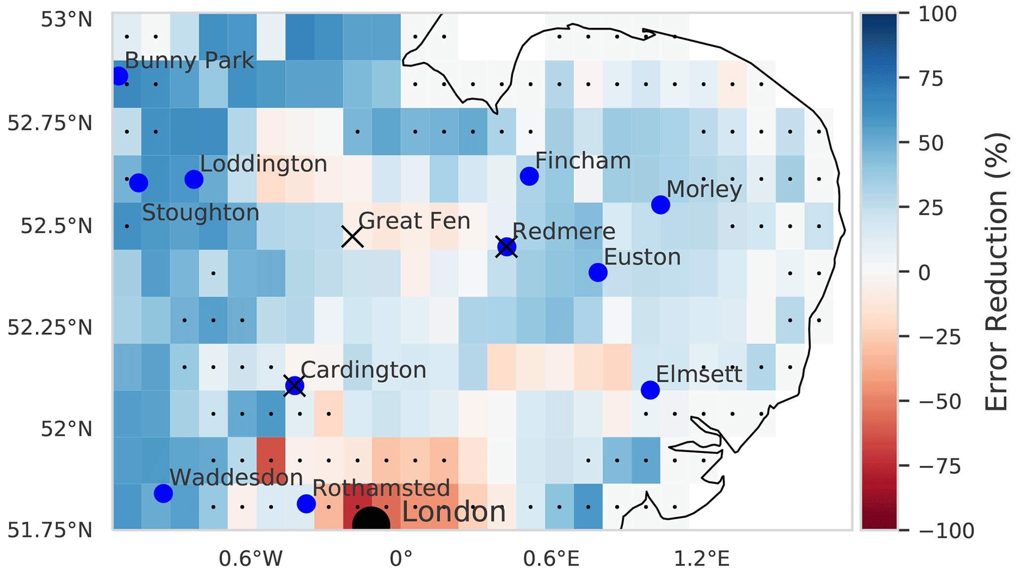
Figure 7Map showing the difference between root mean squared error (RMSE) when JULES spatially aggregated estimates are compared to SMAP observations for the prior and posterior ensemble. Blue corresponds to reductions in RMSE for the posterior ensemble and red to an increase. Grid cells displaying stippling signify low-quality SMAP pixels, which have not been used in the assimilation procedure. Over the whole domain, we find an average reduction in RMSE of 20 % after data assimilation for 2016 and 21 % for 2017.
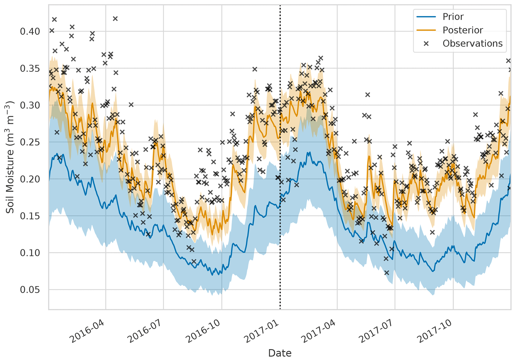
Figure 8Time series of soil moisture for 52.96∘ N, 0.40∘ W. Black crosses: SMAP observations, blue line and shading: prior JULES mean and ensemble spread, orange line and shading: posterior ensemble mean and spread. The dotted black line represents the end of the assimilation window and start of the hindcast period.
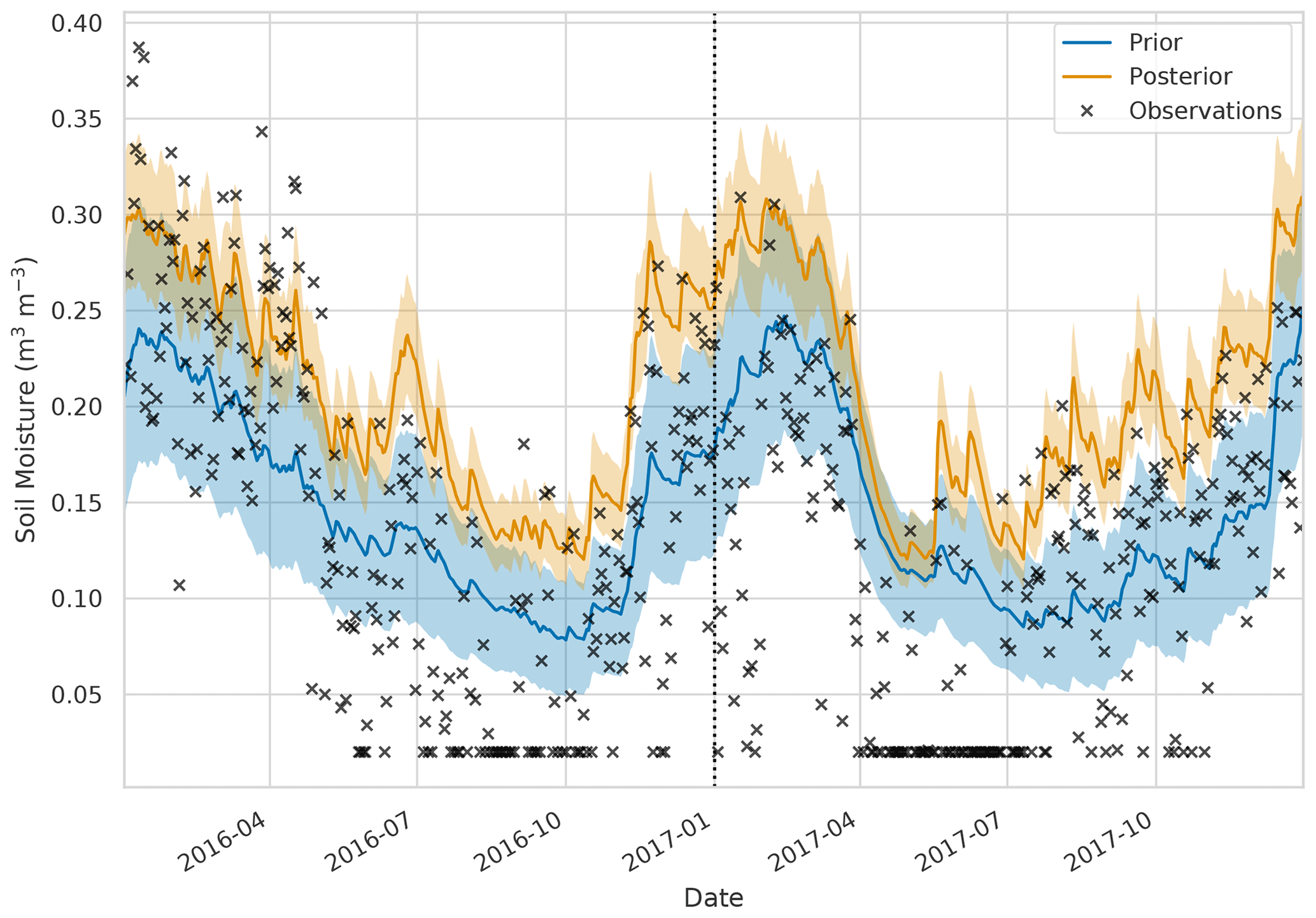
Figure 9Time series of soil moisture for 51.81∘ N 0.17∘ W. Black crosses: SMAP observations, blue line and shading: prior JULES mean and ensemble spread, orange line and shading: posterior ensemble mean and spread. The dotted black line represents the end of the assimilation window and start of the hindcast period.
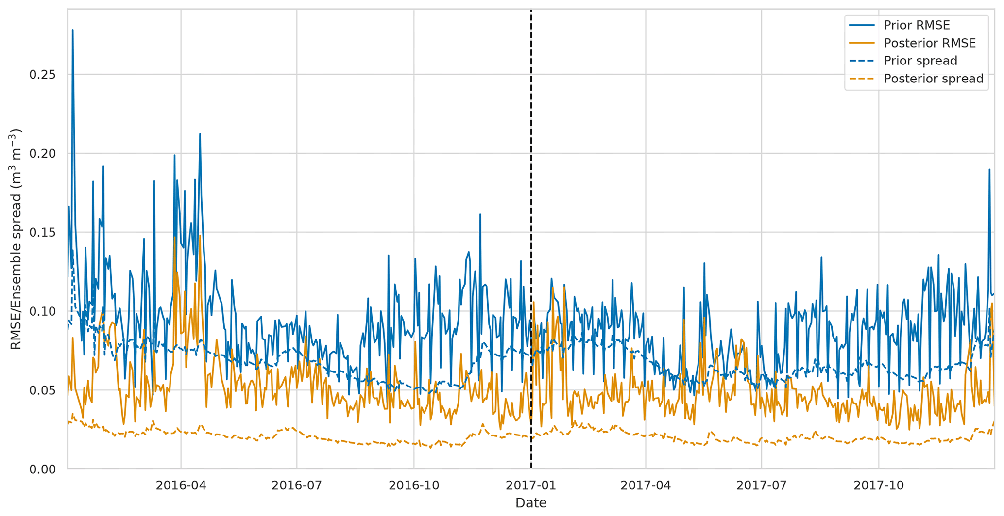
Figure 10 Spatially averaged RMSE and ensemble spread for JULES prior and posterior model estimate. Solid blue line: prior JULES RMSE, dashed blue line: prior JULES ensemble spread, solid orange line: posterior JULES RMSE, dashed orange line: posterior JULES ensemble spread. The dotted black line represents the end of the assimilation window and start of the hindcast period.
3.2 Comparison to COSMOS-UK
After performing the data assimilation procedure, we use the observation operator described in Sect. 2.4 to compare the prior and posterior JULES four-layer soil moisture estimates to the 11 COSMOS probes located in our experiment domain. For each COSMOS site, we select the nearest JULES grid cell to the given site's longitude and latitude. In Fig. 11, we show results at the Cardington COSMOS site; here we can see the posterior JULES estimate is a large improvement on the prior, although some of the driest values are still not captured. From Fig. 11, we can also see there is an increase in evapotranspiration and a decrease in runoff; this effect can also be seen from Fig. 6. Figure 12 shows results for Morley COSMOS site, where both prior and posterior JULES estimates perform similarly; we also have less of an update to evapotranspiration but a decrease in modelled runoff. There are also some sites where even after calibration we still do not capture the COSMOS estimates; Stoughton in Fig. 13 is such an example where both prior and posterior estimates are too dry. However, here the posterior estimate is still much improved from the prior. We also find large increases in evapotranspiration and reductions in runoff for Stoughton. Figure 14 is an example where both prior and posterior perform equally poorly. The fact that the estimates and updates after DA are so different for Figs. 11–14 despite all using the same PTF parameters highlights the effect that the underlying soil properties are having on soil hydraulic conductivity. At all sites, the JULES model predicts top-layer soil temperature well when both prior and posterior estimates are compared to in situ observations. In Table 3, we show summary statistics for soil moisture at the 11 COSMOS sites; we see that when looking over all sites the posterior estimate yields a 16 % increase in correlation, 16 % reduction in unbiased root mean squared error (ubRMSE) and a 22 % reduction in root mean squared error (RMSE) when compared to the prior.
The COSMOS-UK observations we have used for independent validation of the results are representative of depths from 14 cm up to around 40 cm. The SMAP satellite observations, used within the assimilation algorithm to find a new set of pedotransfer functions for the experiment domain, are representative of soil moisture for the top 2.5–5 cm of soil. Therefore the fact that after assimilation we find such a distinct improvement at in situ COSMOS probe locations indicates that although the SMAP observations are only sensitive to shallow depths, by combining these with the JULES model, we are also improving estimates at deeper levels. The large errors in our prior JULES estimates for the COSMOS sites in Figs. 13 and 14 could point towards some systematic bias within the model. However, it is important to note that the COSMOS-UK observations are independent of the data assimilation. For the assimilated SMAP observations, it may be optimal to have errors centred around zero, but for the independent in situ validation data, there will be many competing errors that may make this impossible. There will be errors in the forcing meteorology (here we are using CHESS 1 km forcing data and not observed in situ meteorology), errors in the model grid and its representativity to the in situ location, structural model errors (we currently have no groundwater model in JULES, and some in situ sites may be more groundwater-dominated), errors in the vegetation fractions and many more. At the larger SMAP scale, many of these effects will be minimised when looking at the 9 km spatial scale that is more representative of modelled estimates.

Figure 11Time series of water budget variables and soil temperature at Cardington COSMOS site. Black plus signs: COSMOS-UK observations, grey crosses: SMAP observations for closest 9 km pixel, blue line: prior JULES estimate for closest 1 km grid cell, orange line: posterior JULES estimate for closest 1 km grid cell.
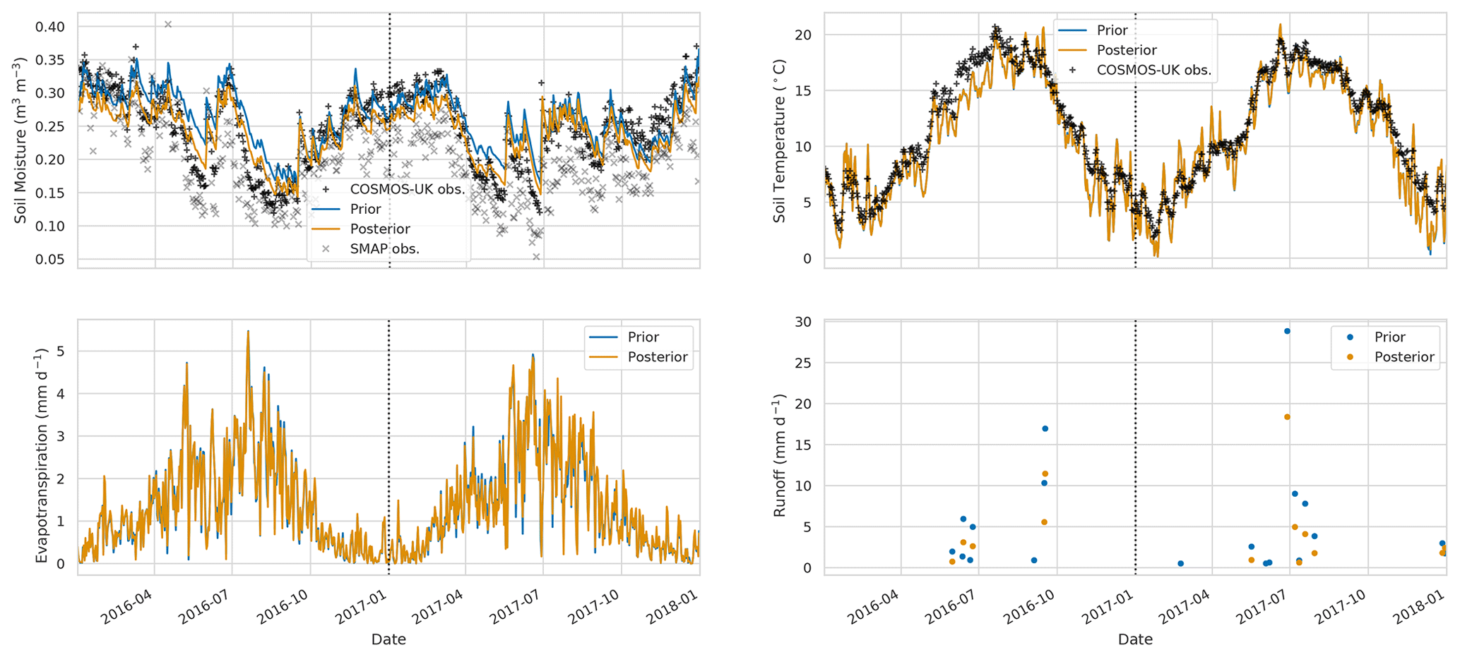
Figure 12Time series of water budget variables and soil temperature at Morley COSMOS site. Black plus signs: COSMOS-UK observations, grey crosses: SMAP observations for closest 9 km pixel, blue line: prior JULES estimate for closest 1 km grid cell, orange line: posterior JULES estimate for closest 1 km grid cell.
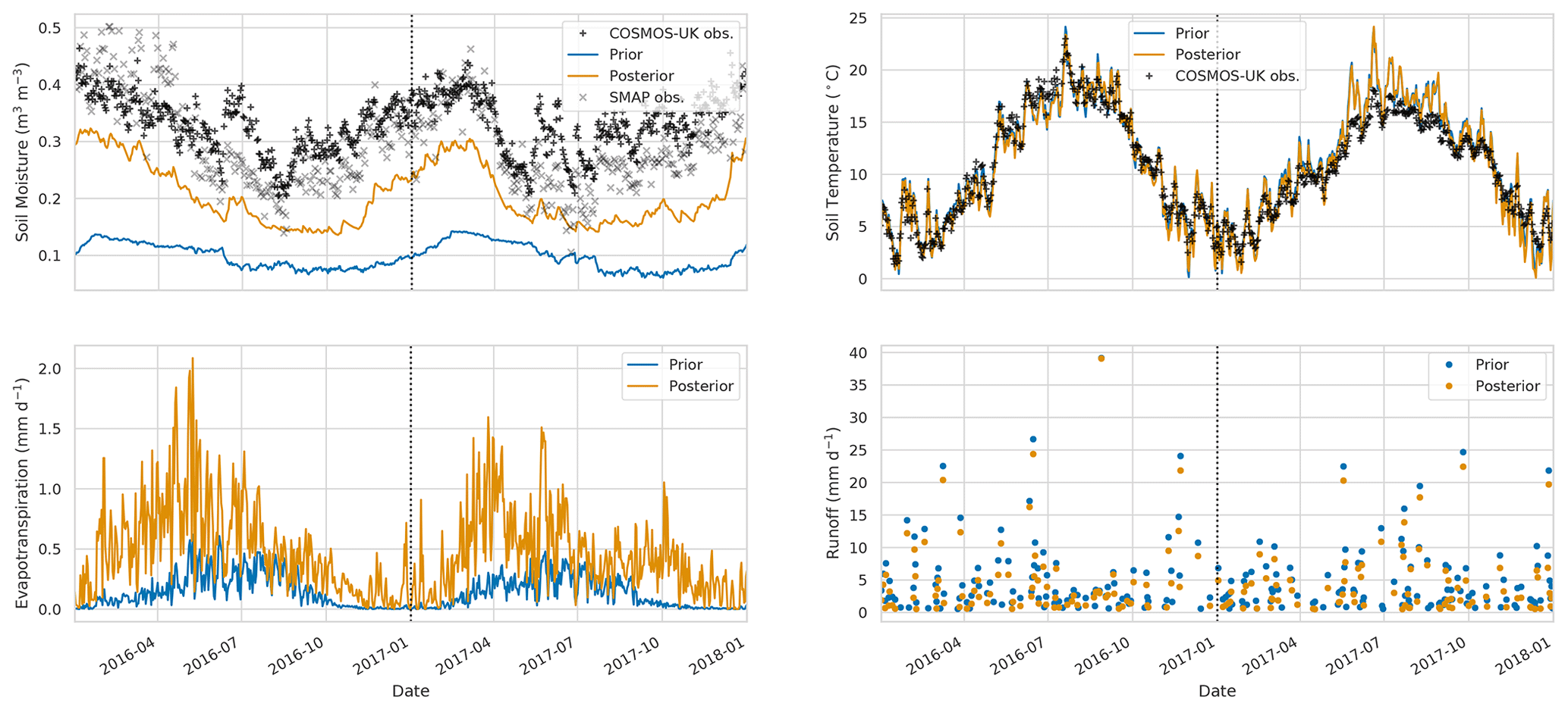
Figure 13Time series of water budget variables and soil temperature at Stoughton COSMOS site. Black plus signs: COSMOS-UK observations, grey crosses: SMAP observations for closest 9 km pixel, blue line: prior JULES estimate for closest 1 km grid cell, orange line: posterior JULES estimate for closest 1 km grid cell.
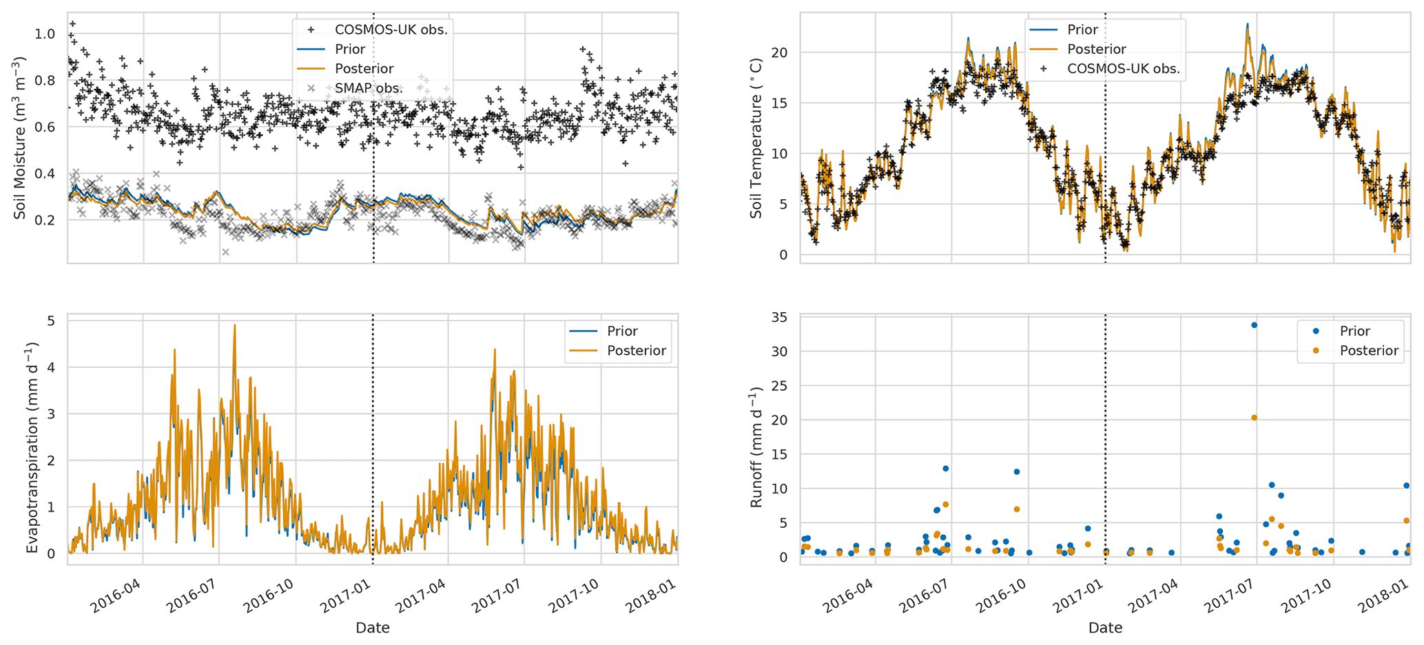
Figure 14Time series of water budget variables and soil temperature at Redmere COSMOS site. Black plus signs: COSMOS-UK observations, grey crosses: SMAP observations for closest 9 km pixel, blue line: prior JULES estimate for closest 1 km grid cell, orange line: posterior JULES estimate for closest 1 km grid cell.
Table 3Summary statistics for comparison of JULES-CHESS soil moisture estimates to COSMOS probe observations over the experiment period. Over all sites, we find a 16 % increase in correlation, 16 % reduction in ubRMSE and 22 % reduction in RMSE after performing the calibration using LAVENDAR.

3.3 Comparison to flux tower observations
In this section, we compare our results to heat flux observations made at three flux tower sites during the experiment period. Although updating the soil parameters and soil moisture in our experiments will have an impact on the modelled heat fluxes, there are multiple model components that will effect the heat flux estimates (vegetation schemes, roughness length parameterisations, etc.), so that improving modelled soil moisture does not necessarily lead to improved modelled heat fluxes. However, if these other model components perform adequately, we should see some improvement in heat flux estimates from improved soil moisture predictions. In Figs. 15 to 17, we show the prior and posterior JULES estimates compared to flux tower observations at each site, alongside the prior and posterior soil moisture for the model grid cell nearest the flux tower. For Fig. 15, we can see that at Cardington for latent heat the posterior JULES estimates move toward the flux tower observations; this is also the case to a lesser degree for sensible heat flux, with these changes corresponding to a large update to the soil moisture trajectory after assimilation. For the Great Fen flux tower site in Fig. 16, we can see we have fewer available observations; at this site we have a smaller update to the soil moisture trajectory after data assimilation with the prior and posterior both matching the SMAP observations well. Even with this slight update to soil moisture at the Great Fen site, we see a moderate improvement in latent and sensible heat flux compared to the observations. We have a similar situation for Redmere in Fig. 17, where a small increment to the soil moisture trajectory corresponds to moderate improvements in the model estimated heat fluxes. In Tables 4 and 5, we show summary statistics for the model performance of latent and sensible heat at the three flux tower sites. From these tables, we find the largest improvement in modelled heat fluxes after data assimilation at the Cardington flux tower site. This also corresponds to the site with the largest improvement in modelled soil moisture. However, even at the Great Fen and Redmere sites where we see less of an impact on modelled soil moisture after data assimilation, we still see some improvement in the modelled heat fluxes. In all cases its seems that JULES slightly under-predicts latent heat and slightly over-predicts sensible heat compared to the observations. As previously noted this under- and over-prediction is likely due to other model components, such as vegetation, for which the model's representation may be different to the truth. This is especially true for the Redmere flux site that is positioned in a cropland with a rotation of maize and lettuce, both of which are not represented in the current configuration of JULES.
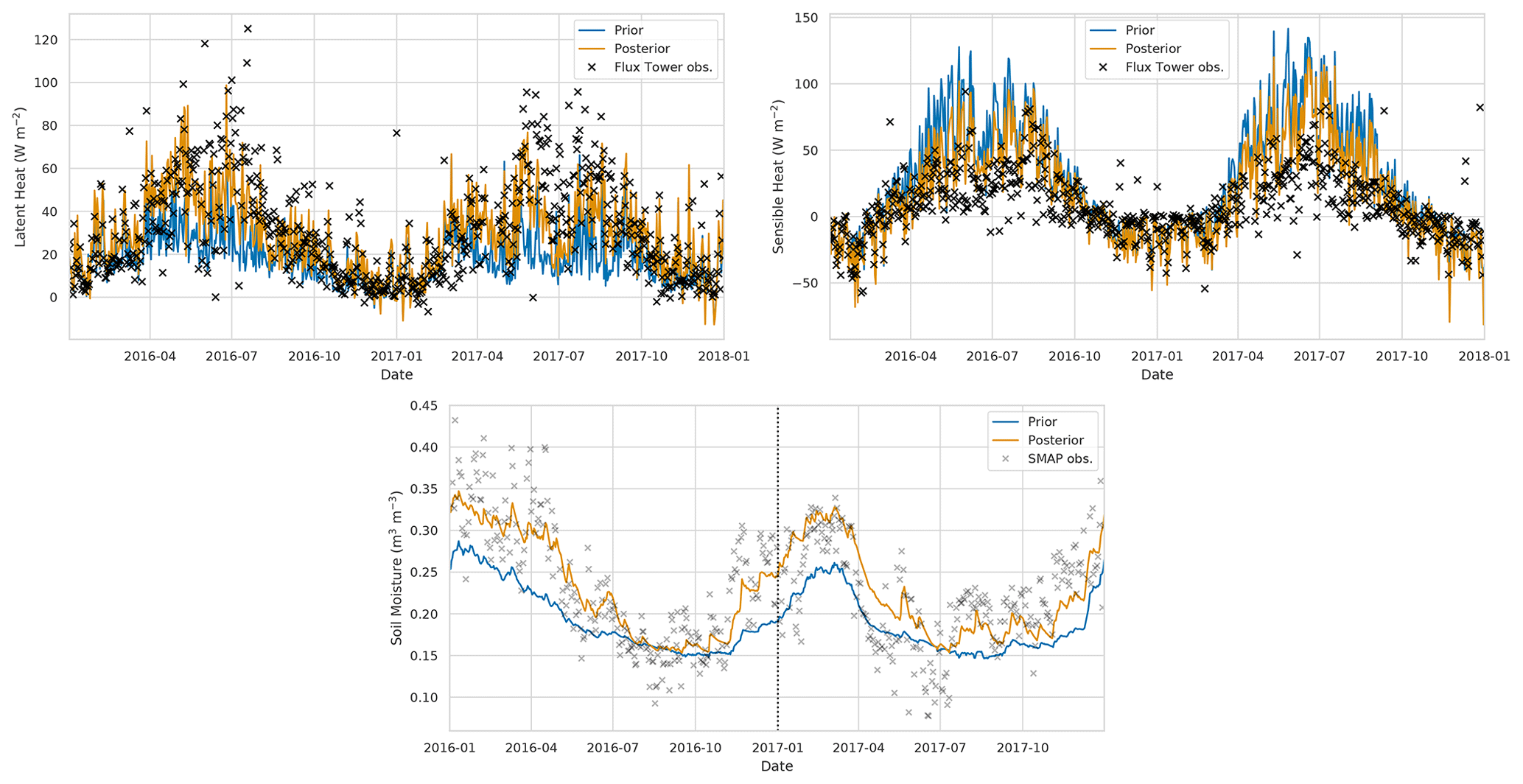
Figure 15Time series of heat flux variables and soil moisture at Cardington flux tower site. Black crosses: flux tower observations, grey crosses: SMAP observations for closest 9 km pixel, blue line: prior JULES estimate for closest 1 km grid cell, orange line: posterior JULES estimate for closest 1 km grid cell.
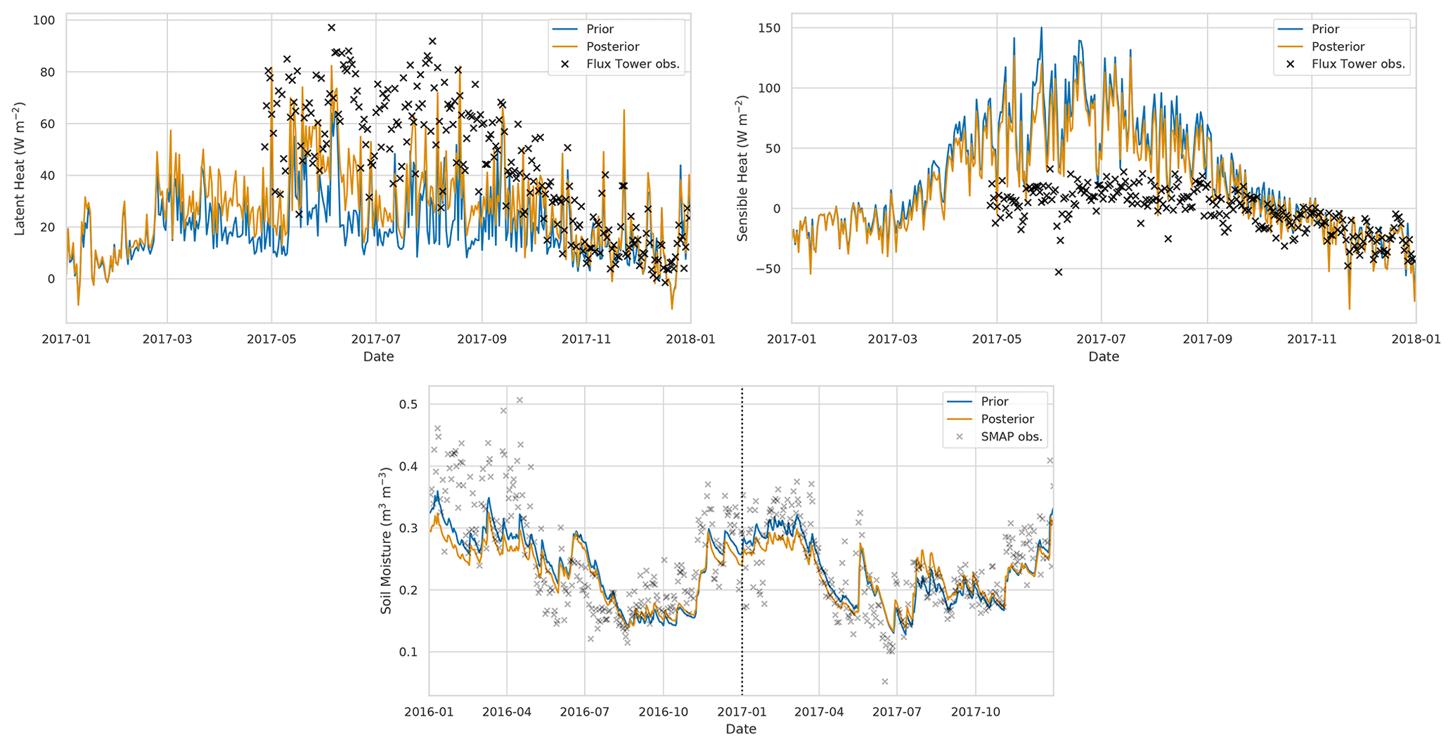
Figure 16Time series of heat flux variables and soil moisture at Great Fen flux tower site. Black crosses: flux tower observations, grey crosses: SMAP observations for closest 9 km pixel, blue line: prior JULES estimate for closest 1 km grid cell, orange line: posterior JULES estimate for closest 1 km grid cell.

Figure 17Time series of heat flux variables and soil moisture at Redmere flux tower site. Black crosses: flux tower observations, grey crosses: SMAP observations for closest 9 km pixel, blue line: prior JULES estimate for closest 1 km grid cell, orange line: posterior JULES estimate for closest 1 km grid cell.
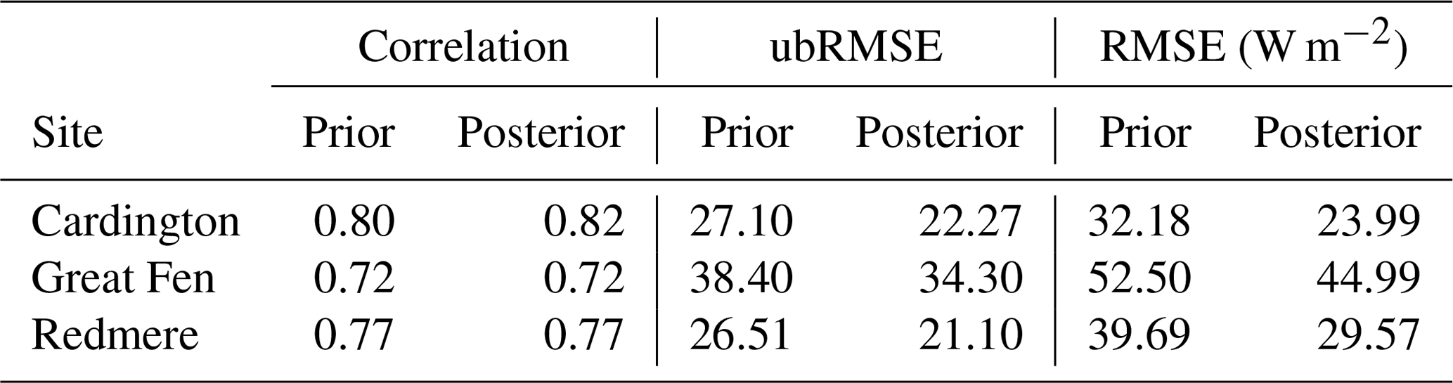
Table 4Summary statistics for comparison of JULES-CHESS latent heat estimates to flux tower observations over the experiment period. Over all sites, we find a 34 % increase in correlation, 15 % reduction in ubRMSE and 26 % reduction in RMSE after performing the calibration using LAVENDAR.
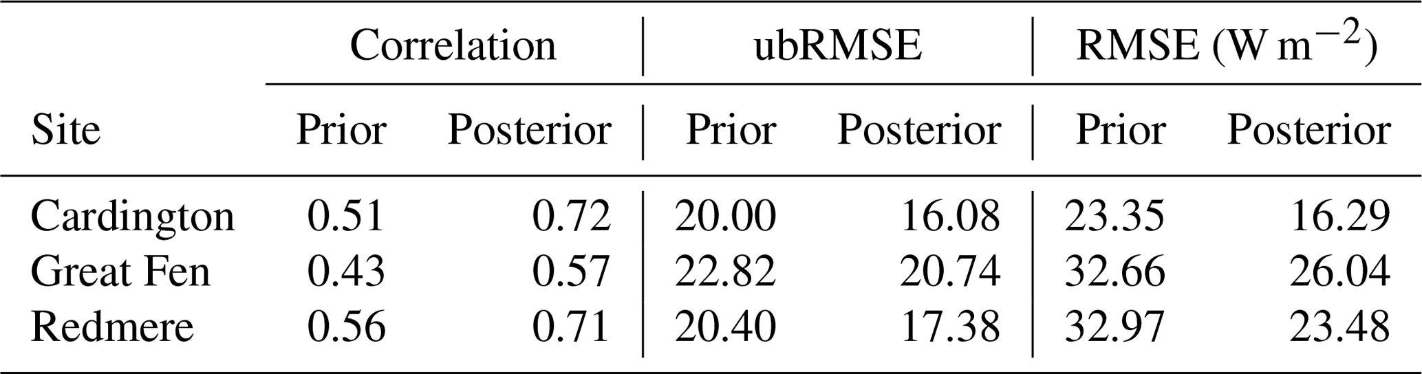
Table 5Summary statistics for comparison of JULES-CHESS sensible heat estimates to flux tower observations over the experiment period. Over all sites, we find a 1 % increase in correlation, 16 % reduction in ubRMSE and 22 % reduction in RMSE after performing the calibration using LAVENDAR.
This study aimed to determine the suitability of satellite observations to optimise pedotransfer functions and improve soil moisture estimates for a land surface model. Currently pedotransfer functions are calibrated through analyses of point soil samples, and it is unclear how these calibrations and their resultant soil model parameters relate to the varying spatial resolutions of modern land surface models. Adding additional information from satellite estimates into the calibration of pedotransfer functions should address a key uncertainty with respect to the larger scales of land surface model estimates.
We used the LAVENDAR hybrid data assimilation framework (Pinnington et al., 2020) to optimise the parameters of the Tóth et al. (2015) pedotransfer functions by combining them with SMAP Level-3 9 km satellite observations and the JULES land surface model run at a 1 km resolution. This framework outputs a single set of PTF parameters valid in space and time by utilising all data at once through the minimisation of a cost function. The optimised pedotransfer functions found after DA were shown to improve model estimates of soil moisture when compared to SMAP data from a different time period (21 % reduction in RMSE) and independent in situ observations from the COSMOS-UK network (16 % increase in correlation, 16 % reduction in ubRMSE and 22 % reduction in RMSE over 11 sites) while also seeing some improvement in modelled sensible and latent heat flux at three independent flux tower sites. This demonstrates that satellite observations can be used to update pedotransfer functions and improve estimates of soil moisture for land surface models. Previous studies have shown that satellite observations can be used to improve model estimates of soil moisture by directly updating soil model parameters on a grid-by-grid basis. Han et al. (2014) used observations from the Soil Moisture Ocean Salinity (SMOS) mission (Kerr et al., 2001) to update parameters of the Community Land Model (CLM) in a local ensemble transform Kalman filter (LETKF) and improved model estimates. Yang et al. (2016) used a variational method to combine observations from the Advanced Microwave Scanning Radiometer for Earth Observing System (AMSR-E) (Kawanishi et al., 2003) with a land surface model to improve estimates over the Tibetan and Mongolian Plateau. Nearing et al. (2010) used calibration techniques to update NOAH land surface model parameters using synthetic aperture radar imagery at a site in Arizona, USA. Our results show similar improvements are achieved by updating PTF parameters with SMAP satellite data. We also demonstrate that information from such satellite observations which are representative of a larger spatial area (9 km) and shallow soil depth (2.5–5 cm) allows us to improve 1 km model estimates at independent COSMOS probe sites. The COSMOS probes are representative of a much smaller spatial scale (∼ 300 m) and a deeper soil layer (14–40 cm), meaning that by combining SMAP observations with the JULES model, we are able to find PTFs that better represent finer spatial scales and deeper soil moisture.
The correlated nature of the PTF parameters in Eq. (1) presents a potential source of equifinality (e.g. both ϕa and ϕc act to increase the magnitude of θsat in the presence of clay soils); this means that we could achieve the same soil hydraulic conductivity with multiple realisations of PTF parameters at any individual grid cell. The effect of this is greatly reduced as we are performing the optimisation over the whole domain and not on a grid-by-grid basis. In effect, this means the unique soil properties at each of the 30 614 model grid cells act as orthogonal constraints within the DA algorithm and reduce the issue of equifinality for the optimised PTF parameters as the DA algorithm is having to fit the assimilated soil moisture observations for many different soil textures at once. It may also be possible to improve results further by including information on such correlations within our prior. Such estimates have been included in a variational DA framework for the carbon cycle and shown to improve posterior estimates (Pinnington et al., 2016). Previous studies have noted the issue of equifinality when optimising soil model parameters on a grid-by-grid basis (Beven, 2001). Samaniego et al. (2010) proposed the multiscale parameter regionalisation method to alleviate this issue by performing a spatial uniforming function and linking parameters at coarser scales to those at finer resolutions. Our technique also allows for a vastly reduced parameter space by moving from updating gridded soil model parameters to instead optimising a single set of pedotransfer function parameters valid in space and time. This could also lead to issues as we are not considering uncertainty in the underlying soil property database (Fischer et al., 2008), which could contain errors (Tifafi et al., 2018). It may be appropriate when performing such a technique at a larger scale that the optimisation is split up into different calibration zones as it has been shown that pedotransfer functions in certain regions can have a different form (e.g. tropical soils; Marthews et al., 2014).
Within the DA procedure used to optimise the PTF parameters, there are uncertainties that have not been explicitly prescribed. There will be inherent bias and errors in both the observations and model. For SMAP, any bias contained in the observations could cause us to retrieve PTF parameters that result in erroneous soil hydraulic conductivities and ultimately degrade the performance of other model components. It has been shown that the Level-3 9 km SMAP observations used here do not have a significant bias (Colliander et al., 2017), especially in temperate regions (Zhang et al., 2019). The fact that after assimilation of the SMAP data we not only reduce the RMSE of JULES compared to SMAP but also reduce the RMSE of JULES compared to independent COSMOS estimates also gives us confidence that the bias in the assimilated SMAP data is relatively low. We have dealt with the many errors contained within our DA cost function by inflating the observation uncertainty within the observation error covariance matrix, as described in Sect. 2.6. However, specifying the errors arising from structural uncertainties and missing processes within the JULES model is difficult. We can see these errors manifesting themselves in our comparisons to COSMOS-UK observations in Figs. 11 to 14. Figure 11 displays results for the Cardington cosmic-ray probe; this site is a level, well-managed grassland with a typical mineral soil and is therefore well modelled by JULES, which has the ability to represent the processes of such a site. Both the Morley and Stoughton sensors (Figs. 12 and 13 respectively) are positioned on arable land with typical mineral soils, and while we model Morley well, we struggle to match the magnitude of the Stoughton observations. It is possible that different management practices at the respective sites are impacting the ability of JULES to predict the observations. In this paper we have not run JULES with its in-built crop model turned on, so that the model will struggle to represent heavily managed crops that behave distinctly from a grassland. The site at which both prior and posterior perform worst is Redmere (Fig. 14); this cosmic-ray probe is again on arable land but with a soil type of peat. In its current configuration, JULES does not model organic soils, and estimates of soil moisture from microwave satellite sensors over peatland are problematic (Zhang et al., 2019), so it is understandable that we are unable to match the much wetter conditions observed at this site. The accuracy of JULES posterior estimates is also contingent on the assimilated SMAP observations, so if SMAP estimates have large errors compared to cosmic-ray probe observations, JULES will be unable to improve from its prior predictions.
In the initial application of this technique, we have focused on a specific region at a high resolution. Here we have utilised 256 processors to run the JULES model ensemble, with each JULES run utilising message parsing interfaces to disaggregate the spatial domain of the model and split the computational load across multiple processors. In this setup, it has taken approximately 1.5 d to complete 100 JULES model runs, with each model being for 30 614 grid cells and over 6 years (2016 to 2017, with a 4-year spin-up). In order to find a set of pedotransfer function parameters valid at the global scale, using the technique presented here, we would need to decrease the spatial resolution. Working at the scale of 0.5∘, we would have approximately 67 000 land grid cells globally. Using our fairly modest experimental setup (and assuming a linear scaling) repetition at the global scale would still only take a little over 3 d. However, it may be beneficial to focus on regional efforts to ensure the optimised pedotransfer functions best reflect the behaviour of local soils. The global domain could then be decomposed into subregions, with specific parameters being found for each distinct region.
Both SMAP and COSMOS-UK observations represent a valuable resource for validation and improvement of land surface models and could be further utilised still. It is possible that our formation of a spatially aggregated observation operator to compare SMAP 9 km estimates to JULES 1 km estimates could be improved upon and that more signal may be coming from the centre of the satellite pixel, so that we could weight these JULES model pixels more highly within the observation operator. In future work, it may also be beneficial to build towards a full radiative transfer scheme on top of JULES to assimilate the raw brightness temperature observations from the SMAP satellite to increase the representativity between the observations and the model and reduce sources of bias that may be introduced by the use of ancillary data in the soil moisture retrieval. Other studies utilising different land surface models have shown this works well (Han et al., 2014; Yang et al., 2016; Lievens et al., 2017). The COSMOS-UK observations could also be used within the data assimilation algorithm, rather than just acting as validation, to capture information on another spatial scale. Much work would be needed here to process and organise site-level driving data and understand the different characteristics of each site before combining these observations with the JULES land surface model.
In this paper, we have focused on the optimisation of pedotransfer function parameters to improve estimates of water balance from land surface models. In other regions across the globe where underlying soil texture maps are highly uncertain, it may be necessary to also consider optimising estimates of soil properties per grid cell, given satellite and in situ observations (Pinnington et al., 2018). This could further increase the skill of estimates in problematic areas. There is also the opportunity to incorporate other streams of observations into the data assimilation procedure. For example, the use of streamflow data could give us a powerful integrated constraint on land surface model estimates of water balance and runoff (Abbaszadeh et al., 2020). Flux tower observations of latent and sensible heat could also provide useful constraints on assimilation outputs. Within the Hydro-JULES project, work is being undertaken to improve the representation of hydrological processes at different scales, especially lateral soil water flow and groundwater. The development of the new JULES groundwater component will allow for the use of observations from the Gravity Recovery and Climate Experiment (GRACE) satellites (Tapley et al., 2004), which have the ability to monitor changes in the Earth's underground water storage. It will be informative to rerun this parameter estimation experiment again as new processes are added to the model to understand the effect on the retrieved pedotransfer function parameters. We will then be able to see where we might be over-fitting these parameters to account for current structural deficiencies within the model (such as the current lack of a groundwater model).
We have presented novel methods for calibrating pedotransfer functions used to create the soil parameter ancillaries of a land surface model by using satellite data from the NASA SMAP mission. After the retrieval of an optimised parameter set, using new hybrid data assimilation techniques, we find an average 20 % reduction in error for JULES model estimates of soil moisture when compared to SMAP satellite estimates. There are still areas which remain problematic such as working over urban locations and peatlands. These will require additional modelling efforts and new model components. The resultant posterior pedotransfer functions also improve the prediction of soil moisture and heat fluxes for the JULES land surface model when compared to independent in situ estimates from the COSMOS-UK network and three flux tower sites. At 11 COSMOS-UK research sites distributed across the experiment domain, we find an average 16 % increase in correlation, 16 % reduction in ubRMSE and a 22 % reduction in RMSE for the posterior pedotransfer functions compared to the prior.
In this Appendix we summarise the process to get the analysis (or posterior) ensemble of extended state variables (variables and parameters). In the case of this paper, the variables and parameters correspond to the 15 PTF parameters in Table 1. The following steps are a recapitulation and continuation of the equations in Pinnington et al. (2018).
Let us start with a background ensemble of Ne joint state–parameter vectors:
In our experiments each corresponds to a unique set of 15 PTF parameters and Ne=50. We can define the sample background (or prior) mean as
and the sample background perturbation matrix as
The ensemble background error covariance matrix is defined by
To reduce the difficulty in finding the ensemble analysis mean, we use an incremental and preconditioned algorithm. “Incremental” means that we express the analysis mean which is a perturbation from the background mean, i.e.
The preconditioned part means that the departure δx can be written by a control variable premultiplied by a conditioning matrix. In particular, we choose the departure vector to be written as a linear combination of the background ensemble of perturbations, i.e.
where wa is a vector of weights, which becomes the object we are solving for in the estimation process. This formulation has been used in several formulations, starting with Bishop et al. (2001) and Wang et al. (2004). We do not use localisation in this work, but in the presence of localisation, it would be applied in the manner of Hunt et al. (2007). This vector of weights is the minimiser of a cost function, which can be written in ensemble space as
with gradient
where are the observations for the whole time window and spatial domain (here 2016 SMAP observations over the east of England, with units m3 m−3), and are the linearised and non-linear observation operator respectively (here the JULES model, which includes both a time integration and conversion into observation space to match the SMAP observations) and is the observation error covariance matrix (here containing the error estimates for the assimilated SMAP observations).
In practice, we do not compute the linearised version of JULES. Instead one can define statistics in the observation space in the following manner. The background ensemble of Ne joint state–parameter vectors in observation space is obtained by applying the observation operator to each ensemble member:
The sample background mean in observation space is
and the sample background perturbation matrix in observation space is
Using these considerations, Eqs. (A7) and (A8) become (approximately)
and
Computing the minimum of the cost function (A12) using gradient (A13) yields the maximum a posteriori estimate wa, which inserted into Eq. (A6) gives us the maximum a posteriori estimate of the parameter and/or state variables xa. The analysis error covariance matrix (Pa) is given by (Evensen, 2003)
where K is the Kalman gain matrix and
Then,
i.e. the analysis ensemble of perturbations can be obtained by a right multiplication of the background ensemble of perturbations multiplied by a matrix of weights defined as
In our case, the matrix square root is computed via Cholesky decomposition. Finally the posterior ensemble of Ne parameter–state vectors (Xa) is constructed as
This posterior parameter ensemble and corresponding set of JULES runs can then be used to provide uncertainty estimates for our posterior model predictions and can also be used in future calibration studies or as an ensemble forecast for state estimation.
The code used in experiments is available from the MetOffice JULES repository (https://code.metoffice.gov.uk/trac/roses-u/browser/b/q/3/5/7/trunk, last access: 29 March 2021) (Pinnington, 2020) under Rose suite number u-bq357. The LAVENDAR data assimilation first release is available here: https://doi.org/10.5281/zenodo.2654853 (Pinnington, 2019).
The supplement related to this article is available online at: https://doi.org/10.5194/hess-25-1617-2021-supplement.
EP designed the data assimilation system and conducted all experiments with input from all co-authors. JA contributed to the underlying mathematical framework. EC wrote the algorithm to compare JULES soil moisture to cosmic-ray probe measurements. ER processed the HWSD and built the initial system for relating soil textural information to the parameters of JULES used in these experiments. EP prepared the manuscript with input from all co-authors.
The authors declare that they have no conflict of interest.
This work was funded by the UK Natural Environment Research Council's Hydro-JULES project (NE/S017380/1). The contribution of Tristan Quaife and Javier Amezcua was funded via the UK National Centre for Earth Observation (NCEO) at the University of Reading (grant no. nceo020004). The authors gratefully acknowledge the provision by UKCEH of hydrometeorological and soil data collected by the COSMOS-UK project.
This research has been supported by the UK Natural Environment Research Council (grant no. NE/S017380/1).
This paper was edited by Harrie-Jan Hendricks Franssen and reviewed by Roland Baatz, Long Zhao, and one anonymous referee.
Abbaszadeh, P., Gavahi, K., and Moradkhani, H.: Multivariate remotely sensed and in-situ data assimilation for enhancing community WRF-Hydro model forecasting, Adv. Water Resour., 145, 103721, https://doi.org/10.1016/j.advwatres.2020.103721, 2020. a
Anderson, J. L. and Anderson, S. L.: A Monte Carlo Implementation of the Nonlinear Filtering Problem to Produce Ensemble Assimilations and Forecasts, Mon. Weather Rev., 127, 2741–2758, https://doi.org/10.1175/1520-0493(1999)127<2741:AMCIOT>2.0.CO;2, 1999. a
Asfaw, D., Black, E., Brown, M., Nicklin, K. J., Otu-Larbi, F., Pinnington, E., Challinor, A., Maidment, R., and Quaife, T.: TAMSAT-ALERT v1: a new framework for agricultural decision support, Geosci. Model Dev., 11, 2353–2371, https://doi.org/10.5194/gmd-11-2353-2018, 2018. a
Baatz, R., Bogena, H., Hendricks Franssen, H.-J., Huisman, J., Qu, W., Montzka, C., and Vereecken, H.: Calibration of a catchment scale cosmic-ray probe network: A comparison of three parameterization methods, J. Hydrol., 516, 231–244, https://doi.org/10.1016/j.jhydrol.2014.02.026, 2014. a, b
Baatz, R., Hendricks Franssen, H.-J., Han, X., Hoar, T., Bogena, H. R., and Vereecken, H.: Evaluation of a cosmic-ray neutron sensor network for improved land surface model prediction, Hydrol. Earth Syst. Sci., 21, 2509–2530, https://doi.org/10.5194/hess-21-2509-2017, 2017. a
Bateni, S. M. and Entekhabi, D.: Relative efficiency of land surface energy balance components, Water Resour. Res., 48, W04510, https://doi.org/10.1029/2011WR011357, 2012. a
Beljaars, A. C. M., Viterbo, P., Miller, M. J., and Betts, A. K.: The Anomalous Rainfall over the United States during July 1993: Sensitivity to Land Surface Parameterization and Soil Moisture Anomalies, Mon. Weather Rev., 124, 362–383, https://doi.org/10.1175/1520-0493(1996)124<0362:TAROTU>2.0.CO;2, 1996. a
Best, M. J., Pryor, M., Clark, D. B., Rooney, G. G., Essery, R. L. H., Ménard, C. B., Edwards, J. M., Hendry, M. A., Porson, A., Gedney, N., Mercado, L. M., Sitch, S., Blyth, E., Boucher, O., Cox, P. M., Grimmond, C. S. B., and Harding, R. J.: The Joint UK Land Environment Simulator (JULES), model description – Part 1: Energy and water fluxes, Geosci. Model Dev., 4, 677–699, https://doi.org/10.5194/gmd-4-677-2011, 2011. a
Beven, K.: How far can we go in distributed hydrological modelling?, Hydrol. Earth Syst. Sci., 5, 1–12, https://doi.org/10.5194/hess-5-1-2001, 2001. a
Beven, K. and Binley, A.: The future of distributed models: Model calibration and uncertainty prediction, Hydrol. Process., 6, 279–298, https://doi.org/10.1002/hyp.3360060305, 1992. a
Bishop, C. H., Etherton, B. J., and Majumdar, S. J.: Adaptive Sampling with the Ensemble Transform Kalman Filter. Part I: Theoretical Aspects, Mon. Weather Rev., 129, 420–436, https://doi.org/10.1175/1520-0493(2001)129<0420:ASWTET>2.0.CO;2, 2001. a
Bocquet, M. and Sakov, P.: Joint state and parameter estimation with an iterative ensemble Kalman smoother, Nonlin. Processes Geophys., 20, 803–818, https://doi.org/10.5194/npg-20-803-2013, 2013. a
Bogena, H. R., Huisman, J. A., Güntner, A., Hübner, C., Kusche, J., Jonard, F., Vey, S., and Vereecken, H.: Emerging methods for noninvasive sensing of soil moisture dynamics from field to catchment scale: a review, WIREs Water, 2, 635–647, https://doi.org/10.1002/wat2.1097, 2015. a
Bormann, N., Bonavita, M., Dragani, R., Eresmaa, R., Matricardi, M., and McNally, A.: Enhancing the impact of IASI observations through an updated observation error covariance matrix, ECMWF Technical Memorandum Number 756, ECMWF, https://doi.org/10.21957/gq8j2gjp7, 2015. a
Botto, A., Belluco, E., and Camporese, M.: Multi-source data assimilation for physically based hydrological modeling of an experimental hillslope, Hydrol. Earth Syst. Sci., 22, 4251–4266, https://doi.org/10.5194/hess-22-4251-2018, 2018. a
Brooks, R. H. and Corey, A. T.: Hydraulic properties of porous media and their relation to drainage design, T. ASAE, 7, 26–28, 1964. a, b
Chen, F., Crow, W. T., Bindlish, R., Colliander, A., Burgin, M. S., Asanuma, J., and Aida, K.: Global-scale evaluation of SMAP, SMOS and ASCAT soil moisture products using triple collocation, Remote Sens. Environ., 214, 1–13, https://doi.org/10.1016/j.rse.2018.05.008, 2018. a
Clark, D. B., Mercado, L. M., Sitch, S., Jones, C. D., Gedney, N., Best, M. J., Pryor, M., Rooney, G. G., Essery, R. L. H., Blyth, E., Boucher, O., Harding, R. J., Huntingford, C., and Cox, P. M.: The Joint UK Land Environment Simulator (JULES), model description – Part 2: Carbon fluxes and vegetation dynamics, Geosci. Model Dev., 4, 701–722, https://doi.org/10.5194/gmd-4-701-2011, 2011. a, b
Clark, P., Roberts, N., Lean, H., Ballard, S. P., and Charlton-Perez, C.: Convection-permitting models: a step-change in rainfall forecasting, Meteorol. Appl., 23, 165–181, https://doi.org/10.1002/met.1538, 2016. a
Colliander, A., Jackson, T., Bindlish, R., Chan, S., Das, N., Kim, S., Cosh, M., Dunbar, R., Dang, L., Pashaian, L., Asanuma, J., Aida, K., Berg, A., Rowlandson, T., Bosch, D., Caldwell, T., Caylor, K., Goodrich, D., al Jassar, H., Lopez-Baeza, E., Martínez-Fernàndez, J., Gonzàlez-Zamora, A., Livingston, S., McNairn, H., Pacheco, A., Moghaddam, M., Montzka, C., Notarnicola, C., Niedrist, G., Pellarin, T., Prueger, J., Pulliainen, J., Rautiainen, K., Ramos, J., Seyfried, M., Starks, P., Su, Z., Zeng, Y., van der Velde, R., Thibeault, M., Dorigo, W., Vreugdenhil, M., Walker, J., Wu, X., Monerris, A., O'Neill, P., Entekhabi, D., Njoku, E., and Yueh, S.: Validation of SMAP surface soil moisture products with core validation sites, Remote Sens. Environ., 191, 215–231, https://doi.org/10.1016/j.rse.2017.01.021, 2017. a, b, c
Cosby, B. J., Hornberger, G. M., Clapp, R. B., and Ginn, T. R.: A Statistical Exploration of the Relationships of Soil Moisture Characteristics to the Physical Properties of Soils, Water Resour. Res., 20, 682–690, https://doi.org/10.1029/WR020i006p00682, 1984. a, b
Courtier, P., Thépaut, J.-N., and Hollingsworth, A.: A strategy for operational implementation of 4D-Var, using an incremental approach, Q. J. Roy. Meteor. Soc., 120, 1367–1387, https://doi.org/10.1002/qj.49712051912, 1994. a
De Lannoy, G. J. M. and Reichle, R. H.: Assimilation of SMOS brightness temperatures or soil moisture retrievals into a land surface model, Hydrol. Earth Syst. Sci., 20, 4895–4911, https://doi.org/10.5194/hess-20-4895-2016, 2016. a
Desilets, D. and Zreda, M.: Footprint diameter for a cosmic-ray soil moisture probe: Theory and Monte Carlo simulations, Water Resour. Res., 49, 3566–3575, https://doi.org/10.1002/wrcr.20187, 2013. a
Draper, C. S., Reichle, R. H., De Lannoy, G. J. M., and Liu, Q.: Assimilation of passive and active microwave soil moisture retrievals, Geophys. Res. Lett., 39, L04401, https://doi.org/10.1029/2011GL050655, 2012. a
Duygu, M. B. and Akyürek, Z.: Using Cosmic-Ray Neutron Probes in Validating Satellite Soil Moisture Products and Land Surface Models, Water, 11, 1362, https://doi.org/10.3390/w11071362, 2019. a
Entekhabi, D., Njoku, E. G., O'Neill, P. E., Kellogg, K. H., Crow, W. T., Edelstein, W. N., Entin, J. K., Goodman, S. D., Jackson, T. J., Johnson, J., Kimball, J., Piepmeier, J. R., Koster, R. D., Martin, N., McDonald, K. C., Moghaddam, M., Moran, S., Reichle, R., Shi, J. C., Spencer, M. W., Thurman, S. W., Tsang, L., and Van Zyl, J.: The Soil Moisture Active Passive (SMAP) Mission, P. IEEE, 98, 704–716, 2010. a, b, c
Evensen, G.: The Ensemble Kalman Filter: theoretical formulation and practical implementation, Ocean Dynam., 53, 343–367, https://doi.org/10.1007/s10236-003-0036-9, 2003. a, b
Evensen, G.: Analysis of iterative ensemble smoothers for solving inverse problems, Computat. Geosci., 22, 885–908, https://doi.org/10.1007/s10596-018-9731-y, 2018. a
Evans, J. G., Ward, H. C., Blake, J. R., Hewitt, E. J., Morrison, R., Fry, M., Ball, L. A., Doughty, L. C., Libre, J. W., Hitt, O. E., Rylett, D., Ellis, R. J., Warwick, A. C., Brooks, M., Parkes, M. A., Wright, G. M. H., Singer, A. C., Boorman, D. B., and Jenkins, A.: Soil water content in southern England derived from a cosmic-ray soil moisture observing system – COSMOS-UK, Hydrol. Process., 30, 4987–4999, https://doi.org/10.1002/hyp.10929, 2016. a
Fischer, G., Nachtergaele, F., Prieler, S., Van Velthuizen, H., Verelst, L., and Wiberg, D.: Global agro-ecological zones assessment for agriculture (GAEZ 2008), IIASA, Laxenburg, and FAO, Rome, Italy, available at: http://www.fao.org/soils-portal/soil-survey/soil-maps-and-databases/harmonized-world-soil-database-v12/en/ (last access: 28 April 2020), 2008. a, b, c, d, e
Fowler, A. M., Dance, S. L., and Waller, J. A.: On the interaction of observation and prior error correlations in data assimilation, Q. J. Roy. Meteor. Soc., 144, 48–62, https://doi.org/10.1002/qj.3183, 2018. a
Fratini, G. and Mauder, M.: Towards a consistent eddy-covariance processing: an intercomparison of EddyPro and TK3, Atmos. Meas. Tech., 7, 2273–2281, https://doi.org/10.5194/amt-7-2273-2014, 2014. a
Han, X., Franssen, H.-J. H., Montzka, C., and Vereecken, H.: Soil moisture and soil properties estimation in the Community Land Model with synthetic brightness temperature observations, Water Resour. Res., 50, 6081–6105, https://doi.org/10.1002/2013WR014586, 2014. a, b, c, d
Hauser, M., Orth, R., and Seneviratne, S. I.: Investigating soil moisture–climate interactions with prescribed soil moisture experiments: an assessment with the Community Earth System Model (version 1.2), Geosci. Model Dev., 10, 1665–1677, https://doi.org/10.5194/gmd-10-1665-2017, 2017. a
Hilton, F., Collard, A., Guidard, V., Randriamampianina, R., and Schwaerz, M.: Assimilation of IASI radiances at European NWP centres, available at: https://www.ecmwf.int/node/15331 (last access: 29 March 2021), 2009. a
Houtekamer, P. L. and Mitchell, H. L.: Data Assimilation Using an Ensemble Kalman Filter Technique, Mon. Weather Rev., 126, 796–811, https://doi.org/10.1175/1520-0493(1998)126<0796:DAUAEK>2.0.CO;2, 1998. a
Howes, K. E., Fowler, A. M., and Lawless, A. S.: Accounting for model error in strong-constraint 4D-Var data assimilation, Q. J. Meteor. Soc., 143, 1227–1240, https://doi.org/10.1002/qj.2996, 2017. a
Hunt, B. R., Kostelich, E. J., and Szunyogh, I.: Efficient data assimilation for spatiotemporal chaos: A local ensemble transform Kalman filter, Physica D, 230, 112–126, 2007. a
Kawanishi, T., Sezai, T., Ito, Y., Imaoka, K., Takeshima, T., Ishido, Y., Shibata, A., Miura, M., Inahata, H., and Spencer, R. W.: The Advanced Microwave Scanning Radiometer for the Earth Observing System (AMSR-E), NASDA's contribution to the EOS for global energy and water cycle studies, IEEE T. Geosci. Remote, 41, 184–194, https://doi.org/10.1109/TGRS.2002.808331, 2003. a
Kerr, Y. H., Waldteufel, P., Wigneron, J., Martinuzzi, J., Font, J., and Berger, M.: Soil moisture retrieval from space: the Soil Moisture and Ocean Salinity (SMOS) mission, IEEE T. Geosci. Remote, 39, 1729–1735, 2001. a, b
Köhli, M., Schrön, M., Zreda, M., Schmidt, U., Dietrich, P., and Zacharias, S.: Footprint characteristics revised for field-scale soil moisture monitoring with cosmic-ray neutrons, Water Resour. Res., 51, 5772–5790, https://doi.org/10.1002/2015WR017169, 2015. a, b, c
Kolassa, J., Reichle, R., and Draper, C.: Merging active and passive microwave observations in soil moisture data assimilation, Remote Sens. Environ., 191, 117–130, 2017. a
Li, C., Lu, H., Yang, K., Han, M., Wright, J., Chen, Y., Yu, L., Xu, S., Huang, X., and Gong, W.: The Evaluation of SMAP Enhanced Soil Moisture Products Using High-Resolution Model Simulations and In-Situ Observations on the Tibetan Plateau, Remote Sens., 10, 535, https://doi.org/10.3390/rs10040535, 2018. a
Lievens, H., Reichle, R. H., Liu, Q., De Lannoy, G. J. M., Dunbar, R. S., Kim, S. B., Das, N. N., Cosh, M., Walker, J. P., and Wagner, W.: Joint Sentinel-1 and SMAP data assimilation to improve soil moisture estimates, Geophys. Res. Lett., 44, 6145–6153, https://doi.org/10.1002/2017GL073904, 2017. a
Liu, Q., Reichle, R. H., Bindlish, R., Cosh, M. H., Crow, W. T., de Jeu, R., De Lannoy, G. J. M., Huffman, G. J., and Jackson, T. J.: The Contributions of Precipitation and Soil Moisture Observations to the Skill of Soil Moisture Estimates in a Land Data Assimilation System, J. Hydrometeorol., 12, 750–765, https://doi.org/10.1175/JHM-D-10-05000.1, 2011. a
Lorenc, A. C. and Rawlins, F.: Why does 4D-Var beat 3D-Var?, Q. J. Roy. Meteor. Soc., 131, 3247–3257, https://doi.org/10.1256/qj.05.85, 2005. a
Marthews, T. R., Quesada, C. A., Galbraith, D. R., Malhi, Y., Mullins, C. E., Hodnett, M. G., and Dharssi, I.: High-resolution hydraulic parameter maps for surface soils in tropical South America, Geosci. Model Dev., 7, 711–723, https://doi.org/10.5194/gmd-7-711-2014, 2014. a
Martinez-de la Torre, A., Blyth, E., and Robinson, E.: Water, carbon and energy fluxes simulation for Great Britain using the JULES Land Surface Model and the Climate Hydrology and Ecology research Support System, meteorology dataset (1961–2015) [CHESS-land], https://doi.org/10.5285/c76096d6-45d4-4a69-a310-4c67f8dcf096, 2018. a
Martínez-de la Torre, A., Blyth, E. M., and Weedon, G. P.: Using observed river flow data to improve the hydrological functioning of the JULES land surface model (vn4.3) used for regional coupled modelling in Great Britain (UKC2), Geosci. Model Dev., 12, 765–784, https://doi.org/10.5194/gmd-12-765-2019, 2019. a
Maurer, E. P. and Lettenmaier, D. P.: Potential Effects of Long-Lead Hydrologic Predictability on Missouri River Main-Stem Reservoirs, J. Climate, 17, 174–186, https://doi.org/10.1175/1520-0442(2004)017<0174:PEOLHP>2.0.CO;2, 2004. a
Minamide, M. and Zhang, F.: Adaptive Observation Error Inflation for Assimilating All-Sky Satellite Radiance, Mon. Weather Rev., 145, 1063–1081, https://doi.org/10.1175/MWR-D-16-0257.1, 2017. a
Mizukami, N., Clark, M. P., Newman, A. J., Wood, A. W., Gutmann, E. D., Nijssen, B., Rakovec, O., and Samaniego, L.: Towards seamless large-domain parameter estimation for hydrologic models, Water Resour. Res., 53, 8020–8040, https://doi.org/10.1002/2017WR020401, 2017. a
Montzka, C., Moradkhani, H., Weihermüller, L., Franssen, H.-J. H., Canty, M., and Vereecken, H.: Hydraulic parameter estimation by remotely-sensed top soil moisture observations with the particle filter, J. Hydrol., 399, 410–421, https://doi.org/10.1016/j.jhydrol.2011.01.020, 2011. a
Montzka, C., Bogena, H. R., Zreda, M., Monerris, A., Morrison, R., Muddu, S., and Vereecken, H.: Validation of Spaceborne and Modelled Surface Soil Moisture Products with Cosmic-Ray Neutron Probes, Remote Sens., 9, 103, https://doi.org/10.3390/rs9020103, 2017. a
Moradkhani, H., Sorooshian, S., Gupta, H. V., and Houser, P. R.: Dual state-parameter estimation of hydrological models using ensemble Kalman filter, Adv. Water Resour., 28, 135–147, https://doi.org/10.1016/j.advwatres.2004.09.002, 2005. a, b
Morrison, R., Cooper, H., Cumming, A., Evans, C., Thornton, J., Winterbourn, J., Rylett, D., and Jones, D.: Eddy covariance measurements of carbon dioxide, energy and water fluxes at a cropland and a grassland on lowland peat soils, East Anglia, UK, 2016–2019, UK Centre for Ecology and Hydrology data set, https://doi.org/10.5285/2fe84b80-117a-4b19-a1f5-71bbd1dba9c9, 2020. a
Nearing, G. S., Moran, M. S., Thorp, K. R., Collins, C. D. H., and Slack, D. C.: Likelihood parameter estimation for calibrating a soil moisture model using radar bakscatter, Remote Sens. Environ., 114, 2564–2574, https://doi.org/10.1016/j.rse.2010.05.031, 2010. a, b
Osborne, S. R. and Weedon, G. P.: Observations and Modeling of Evapotranspiration and Dewfall during the 2018 Meteorological Drought in Southern England, J. Hydrometeorol., 22, 279–295, https://doi.org/10.1175/JHM-D-20-0148.1, 2021. a
Papale, D., Reichstein, M., Aubinet, M., Canfora, E., Bernhofer, C., Kutsch, W., Longdoz, B., Rambal, S., Valentini, R., Vesala, T., and Yakir, D.: Towards a standardized processing of Net Ecosystem Exchange measured with eddy covariance technique: algorithms and uncertainty estimation, Biogeosciences, 3, 571–583, https://doi.org/10.5194/bg-3-571-2006, 2006. a
Peng, J., Pinnington, E., Robinson, E., Evans, J., Quaife, T., Harris, P., and Blyth, E.: A high-resolution soil moisture dataset from merged model and Earth observation data in Great Britain, Remote Sens. Environ., in review, 2021. a
Pinnington, E.: pyearthsci/lavendar: First release of LaVEnDAR software (Version v1.0.0), Zenodo, https://doi.org/10.5281/zenodo.2654853, 2019. a
Pinnington, E.: LAVENDAR Rose-suite repository, Met-Office trac system, availalbe at: https://code.metoffice.gov.uk/trac/roses-u/browser/b/q/3/5/7/trunk (last access: 29 March 2021), 2020. a
Pinnington, E., Quaife, T., and Black, E.: Impact of remotely sensed soil moisture and precipitation on soil moisture prediction in a data assimilation system with the JULES land surface model, Hydrol. Earth Syst. Sci., 22, 2575–2588, https://doi.org/10.5194/hess-22-2575-2018, 2018. a, b, c
Pinnington, E., Quaife, T., Lawless, A., Williams, K., Arkebauer, T., and Scoby, D.: The Land Variational Ensemble Data Assimilation Framework: LAVENDAR v1.0.0, Geosci. Model Dev., 13, 55–69, https://doi.org/10.5194/gmd-13-55-2020, 2020. a, b, c
Pinnington, E. M., Casella, E., Dance, S. L., Lawless, A. S., Morison, J. I., Nichols, N. K., Wilkinson, M., and Quaife, T. L.: Investigating the role of prior and observation error correlations in improving a model forecast of forest carbon balance using Four-dimensional Variational data assimilation, Agr. Forest Meteorol., 228/229, 299–314, https://doi.org/10.1016/j.agrformet.2016.07.006, 2016. a
Pitman, A. J., Henderson-Sellers, A., Desborough, C. E., Yang, Z. L., Abramopoulos, F., Boone, A., Dickinson, R. E., Gedney, N., Koster, R., Kowalczyk, E., Lettenmaier, D., Liang, X., Mahfouf, J. F., Noilhan, J., Polcher, J., Qu, W., Robock, A., Rosenzweig, C., Schlosser, C. A., Shmakin, A. B., Smith, J., Suarez, M., Verseghy, D., Wetzel, P., Wood, E., and Xue, Y.: Key results and implications from phase 1(c) of the Project for Intercomparison of Land-surface Parametrization Schemes, Clim. Dynam., 15, 673–684, https://doi.org/10.1007/s003820050309, 1999. a
Rasmy, M., Koike, T., Boussetta, S., Lu, H., and Li, X.: Development of a Satellite Land Data Assimilation System Coupled With a Mesoscale Model in the Tibetan Plateau, IEEE T. Geosci. Remote, 49, 2847–2862, 2011. a, b
Reichle, R. H., De Lannoy, G. J. M., Liu, Q., Ardizzone, J. V., Colliander, A., Conaty, A., Crow, W., Jackson, T. J., Jones, L. A., Kimball, J. S., Koster, R. D., Mahanama, S. P., Smith, E. B., Berg, A., Bircher, S., Bosch, D., Caldwell, T. G., Cosh, M., Gonzàlez-Zamora, A., Holifield Collins, C. D., Jensen, K. H., Livingston, S., Lopez-Baeza, E., Martínez-Fernàndez, J., McNairn, H., Moghaddam, M., Pacheco, A., Pellarin, T., Prueger, J., Rowlandson, T., Seyfried, M., Starks, P., Su, Z., Thibeault, M., van der Velde, R., Walker, J., Wu, X., and Zeng, Y.: Assessment of the SMAP Level-4 Surface and Root-Zone Soil Moisture Product Using In Situ Measurements, J. Hydrometeorol., 18, 2621–2645, https://doi.org/10.1175/JHM-D-17-0063.1, 2017. a
Reichstein, M., Falge, E., Baldocchi, D., Papale, D., Aubinet, M., Berbigier, P., Bernhofer, C., Buchmann, N., Gilmanov, T., Granier, A., Grünwald, T., Havránková, K., Ilvesniemi, H., Janous, D., Knohl, A., Laurila, T., Lohila, A., Loustau, D., Matteucci, G., Meyers, T., Miglietta, F., Ourcival, J.-M., Pumpanen, J., Rambal, S., Rotenberg, E., Sanz, M., Tenhunen, J., Seufert, G., Vaccari, F., Vesala, T., Yakir, D., and Valentini, R.: On the separation of net ecosystem exchange into assimilation and ecosystem respiration: review and improved algorithm, Glob. Change Biol., 11, 1424–1439, https://doi.org/10.1111/j.1365-2486.2005.001002.x, 2005. a, b
Reichstein, M., Moffat, A., Wutzler, T., and Sickel, K.: REddyProc: Data processing and plotting utilities of (half-) hourly eddy-covariance measurements, R package version 0.6-0/r9, available at: https://cran.r-project.org/web/packages/REddyProc/index.html (last access: 29 March 2021), 2014. a
Ridler, M.-E., Zhang, D., Madsen, H., Kidmose, J., Refsgaard, J. C., and Jensen, K. H.: Bias-aware data assimilation in integrated hydrological modelling, Hydrol. Res., 49, 989–1004, https://doi.org/10.2166/nh.2017.117, 2017. a
Robinson, E., Blyth, E., Clark, D., Comyn-Platt, E., Finch, J., and Rudd, A.: Climate hydrology and ecology research support system meteorology dataset for Great Britain (1961–2015) [CHESS-met] v1.2, https://doi.org/10.5285/b745e7b1-626c-4ccc-ac27-56582e77b900, 2017. a
Rosolem, R., Hoar, T., Arellano, A., Anderson, J. L., Shuttleworth, W. J., Zeng, X., and Franz, T. E.: Translating aboveground cosmic-ray neutron intensity to high-frequency soil moisture profiles at sub-kilometer scale, Hydrol. Earth Syst. Sci., 18, 4363–4379, https://doi.org/10.5194/hess-18-4363-2014, 2014. a
Samaniego, L., Kumar, R., and Attinger, S.: Multiscale parameter regionalization of a grid-based hydrologic model at the mesoscale, Water Resour. Res., 46, W05523, https://doi.org/10.1029/2008WR007327, 2010. a
Sawada, Y. and Koike, T.: Simultaneous estimation of both hydrological and ecological parameters in an ecohydrological model by assimilating microwave signal, J. Geophys. Res.-Atmos., 119, 8839–8857, https://doi.org/10.1002/2014JD021536, 2014. a, b
Schaap, M. G., Nemes, A., and van Genuchten, M. T.: Comparison of Models for Indirect Estimation of Water Retention and Available Water in Surface Soils, Vadose Zone J., 3, 1455–1463, https://doi.org/10.2136/vzj2004.1455, 2004. a
Shuttleworth, J., Rosolem, R., Zreda, M., and Franz, T.: The COsmic-ray Soil Moisture Interaction Code (COSMIC) for use in data assimilation, Hydrol. Earth Syst. Sci., 17, 3205–3217, https://doi.org/10.5194/hess-17-3205-2013, 2013. a
Stanley, S., Antoniou, V., Ball, L., Bennett, E., Blake, J., Boorman, D., Brooks, M., Clarke, M., Cooper, H., Cowan, N., Evans, J., Farrand, P., Fry, M., Hitt, O., Jenkins, A., Kral, F., Lord, W., Morrison, R., Nash, G., Rylett, D., Scarlett, P., Swain, O., Thornton, J., Trill, E., Warwick, A., and Winterbourn, J.: Daily and sub-daily hydrometeorological and soil data (2013–2017) [COSMOS-UK], https://doi.org/10.5285/a6012796-291c-4fd6-a7ef-6f6ed0a6cfa5, 2019. a, b
Stewart, L. M., Dance, S. L., Nichols, N. K., Eyre, J. R., and Cameron, J.: Estimating interchannel observation-error correlations for IASI radiance data in the Met Office system†, Q. J. Roy. Meteor. Soc., 140, 1236–1244, https://doi.org/10.1002/qj.2211, 2014. a
Tapley, B. D., Bettadpur, S., Ries, J. C., Thompson, P. F., and Watkins, M. M.: GRACE Measurements of Mass Variability in the Earth System, Science, 305, 503–505, https://doi.org/10.1126/science.1099192, 2004. a
Thiemann, M., Trosset, M., Gupta, H., and Sorooshian, S.: Bayesian recursive parameter estimation for hydrologic models, Water Resour. Res., 37, 2521–2535, https://doi.org/10.1029/2000WR900405, 2001. a
Tifafi, M., Guenet, B., and Hatté, C.: Large Differences in Global and Regional Total Soil Carbon Stock Estimates Based on SoilGrids, HWSD, and NCSCD: Intercomparison and Evaluation Based on Field Data From USA, England, Wales, and France, Global Biogeochem. Cy., 32, 42–56, https://doi.org/10.1002/2017GB005678, 2018. a
Tóth, B., Weynants, M., Nemes, A., Makó, A., Bilas, G., and Tóth, G.: New generation of hydraulic pedotransfer functions for Europe, Eur. J. Soil Sci., 66, 226–238, https://doi.org/10.1111/ejss.12192, 2015. a, b, c, d, e, f, g, h, i, j, k, l
van Genuchten, M. T.: A Closed-form Equation for Predicting the Hydraulic Conductivity of Unsaturated Soils, Soil Sci. Soc. Am. J., 44, 892–898, https://doi.org/10.2136/sssaj1980.03615995004400050002x, 1980. a, b, c, d, e, f, g, h, i
Van Looy, K., Bouma, J., Herbst, M., Koestel, J., Minasny, B., Mishra, U., Montzka, C., Nemes, A., Pachepsky, Y. A., Padarian, J., Schaap, M. G., Tóth, B., Verhoef, A., Vanderborght, J., van der Ploeg, M. J., Weihermüller, L., Zacharias, S., Zhang, Y., and Vereecken, H.: Pedotransfer Functions in Earth System Science: Challenges and Perspectives, Rev. Geophys., 55, 1199–1256, https://doi.org/10.1002/2017RG000581, 2017. a
Vrugt, J. A., Gupta, H. V., Bouten, W., and Sorooshian, S.: A Shuffled Complex Evolution Metropolis algorithm for optimization and uncertainty assessment of hydrologic model parameters, Water Resour. Res., 39, 1201, https://doi.org/10.1029/2002WR001642, 2003. a
Wagner, W., Hahn, S., Kidd, R., Melzer, T., Bartalis, Z., Hasenauer, S., Figa-Saldaña, J., de Rosnay, P., Jann, A., Schneider, S., Komma, J., Kubu, G., Brugger, K., Aubrecht, C., Züger, J., Gangkofner, U., Kienberger, S., Brocca, L., Wang, Y., Blöschl, G., Eitzinger, J., Steinnocher, K., Zeil, P., and Rubel, F.: The ASCAT Soil Moisture Product: A Review of its Specifications, Validation Results, and Emerging Applications, Meteorol. Z., 22, 5–33, https://doi.org/10.1127/0941-2948/2013/0399, 2013. a
Walker, J. P., Willgoose, G. R., and Kalma, J. D.: In situ measurement of soil moisture: a comparison of techniques, J. Hydrol., 293, 85–99, https://doi.org/10.1016/j.jhydrol.2004.01.008, 2004. a
Wang, P., Li, J., Li, Z., Lim, A. H. N., Li, J., and Goldberg, M. D.: Impacts of Observation Errors on Hurricane Forecasts When Assimilating Hyperspectral Infrared Sounder Radiances in Partially Cloudy Skies, J. Geophys. Res.-Atmos., 124, 10802–10813, https://doi.org/10.1029/2019JD031029, 2019. a
Wang, X., Bishop, C. H., and Julier, S. J.: Which Is Better, an Ensemble of Positive–Negative Pairs or a Centered Spherical Simplex Ensemble?, Mon. Weather Rev., 132, 1590–1605, https://doi.org/10.1175/1520-0493(2004)132<1590:WIBAEO>2.0.CO;2, 2004. a
Wösten, J., Lilly, A., Nemes, A., and Le Bas, C.: Development and use of a database of hydraulic properties of European soils, Geoderma, 90, 169–185, https://doi.org/10.1016/S0016-7061(98)00132-3, 1999. a, b
Yang, K., Zhu, L., Chen, Y., Zhao, L., Qin, J., Lu, H., Tang, W., Han, M., Ding, B., and Fang, N.: Land surface model calibration through microwave data assimilation for improving soil moisture simulations, J. Hydrol., 533, 266–276, https://doi.org/10.1016/j.jhydrol.2015.12.018, 2016. a, b, c, d
Zhang, R., Kim, S., and Sharma, A.: A comprehensive validation of the SMAP Enhanced Level-3 Soil Moisture product using ground measurements over varied climates and landscapes, Remote Sens. Environ., 223, 82–94, https://doi.org/10.1016/j.rse.2019.01.015, 2019. a, b, c, d
Zheng, D., Li, X., Wang, X., Wang, Z., Wen, J., van der Velde, R., Schwank, M., and Su, Z.: Sampling depth of L-band radiometer measurements of soil moisture and freeze-thaw dynamics on the Tibetan Plateau, Remote Sens. Environ., 226, 16–25, https://doi.org/10.1016/j.rse.2019.03.029, 2019. a
Zreda, M., Desilets, D., Ferré, T. P. A., and Scott, R. L.: Measuring soil moisture content non-invasively at intermediate spatial scale using cosmic-ray neutrons, Geophys. Res. Lett., 35, L21402, https://doi.org/10.1029/2008GL035655, 2008. a, b
Zreda, M., Shuttleworth, W. J., Zeng, X., Zweck, C., Desilets, D., Franz, T., and Rosolem, R.: COSMOS: the COsmic-ray Soil Moisture Observing System, Hydrol. Earth Syst. Sci., 16, 4079–4099, https://doi.org/10.5194/hess-16-4079-2012, 2012. a