The benefit of brightness temperature assimilation for the SMAP Level-4 surface and root-zone soil moisture analysis

The Soil Moisture Active Passive (SMAP) Level-4 (L4) product provides global estimates of surface soil moisture (SSM) and root-zone soil moisture (RZSM) via the assimilation of SMAP brightness temperature (T_b) observations into the NASA Catchment Land Surface Model (CLSM). Here, using in situ measurements from 2474 sites in China, we evaluate the performance of soil moisture estimates from the L4 data assimilation (DA) system and from a baseline “open-loop” (OL) simulation of CLSM without T_b assimilation. Using random forest regression, the efficiency of the L4 DA system (i.e., the performance improvement in DA relative to OL) is attributed to eight control factors related to the CLSM as well as τ–ω radiative transfer model (RTM) components of the L4 system. Results show that the Spearman rank correlation (R) for L4 SSM with in situ measurements increases for 77 % of the in situ measurement locations (relative to that of OL), with an average R increase of approximately 14 % (ΔR=0.056). RZSM skill is improved for about 74 % of the in situ measurement locations, but the average R increase for RZSM is only 7 % (ΔR=0.034). Results further show that the SSM DA skill improvement is most strongly related to the difference between the RTM-simulated T_b and the SMAP T_b observation, followed by the error in precipitation forcing data and estimated microwave soil roughness parameter h. For the RZSM DA skill improvement, these three dominant control factors remain the same, although the importance of soil roughness exceeds that of the T_b simulation error, as the soil roughness strongly affects the ingestion of DA increments and further propagation to the subsurface. For the skill of the L4 and OL estimates themselves, the top two control factors are the precipitation error and the SSM–RZSM coupling strength error, both of which are related to the CLSM component of the L4 system. Finally, we find that the L4 system can effectively filter out errors in precipitation. Therefore, future development of the L4 system should focus on improving the characterization of the SSM–RZSM coupling strength.

1 Introduction

Soil moisture modulates water and energy feedback between the land surface and the lower atmosphere by determining the partitioning of incoming net radiation into latent and sensible heat (Seneviratne et al., 2010, 2013). High-quality, global-scale soil moisture products have become increasingly available in recent years. In particular, the L-band NASA Soil Moisture Active Passive (SMAP) satellite mission (Entekhabi et al., 2010; Piepmeier et al., 2017) has significantly improved the skill of available, global-scale soil moisture products. However, the SMAP observations contain temporal data gaps and are only representative of conditions within only the first 5 cm of the vertical soil moisture column (Entekhabi et al., 2010). To address these limitations, the SMAP Level-4 surface and root-zone soil moisture (L4) algorithm assimilates SMAP brightness temperature (T_b) observations into the NASA Catchment Land Surface Model (CLSM) to derive an analysis of surface (0–5 cm) and root-zone (0–100 cm) soil moisture estimates with global, 3-hourly coverage (Reichle et al., 2017a, b, 2019).

However, the performance of a land data assimilation (DA) system is sensitive to the DA parameterization and requires careful assessment. For instance, Reichle et al. (2008) demonstrate that DA based on incorrect assumptions of modeling errors and observation errors can degrade soil moisture estimates, compared with the case of not performing DA, which is commonly referred to as the “open-loop” (OL) baseline. Theoretically, the optimality of DA can be evaluated using so-called “innovations”, or observation-minus-forecast residuals; however, an investigation of the innovations alone is often insufficient to determine if the soil moisture analysis is optimal, as the innovations are affected by multiple factors (Crow and Van Loon, 2006).

Recently, Dong et al. (2019a) proposed a novel statistical framework for evaluating the performance of a soil moisture DA system. Specifically, they demonstrated that the relative skill of surface soil moisture (SSM) estimates acquired with and without DA can be estimated using the ratio of their correlations with just one noisy but independent ancillary remote sensing product. This approach was applied to the SMAP L4 system using Advanced Scatterometer soil moisture retrievals. Their results show that the benefit of SMAP DA is closely related to densities of both rain gauge and vegetation. Generally, higher rain gauge density indicates lower error in precipitation forcing, and lower vegetation density indicates higher background model performance – both conditions lead to reduced SMAP DA benefit. However, due to the limited availability of independent root-zone soil moisture (RZSM) products for performing statistical error estimation, this method is only applicable for SSM estimates.

Relative to SSM, the efficiency of assimilating land surface observations to improve RZSM is complicated by model structural error that affects the ability of the DA to update unobserved model states. For instance, Kumar et al. (2009) identified the surface–root zone coupling strength, which is the result of a model-dependent representation of processes related to the partitioning of rainfall into infiltration, runoff, and evaporation components, as an important factor for determining RZSM improvement associated with the assimilation of SSM retrievals. Their synthetic experiments suggest that, faced with unknown true subsurface physics, overestimating the surface–root zone coupling in the land model is a more robust strategy for obtaining skill improvements in the root zone than underestimating the coupling. Likewise, Chen et al. (2011) suggested that the Soil and Water Assessment Tool significantly under-predicts the magnitude of vertical soil water coupling in the Cobb Creek Watershed in southwestern Oklahoma, USA, and this lack of coupling impedes the ability of DA to effectively update soil moisture in deep layers, groundwater flow, and surface runoff. In the context of the present paper, the evaluation of L4 RZSM estimates has been limited to SMAP core validation and sparse network sites (Reichle et al., 2017a, b, 2019). With such limited validation sites, the RZSM skill of the L4 product at the global scale remains uncertain.

The primary objective of this study is to assess the DA skill improvement of the L4 product, i.e., the performance improvement in L4 DA results relative to the OL baseline, and to further determine how DA skill improvement varies as a function of the major aspects in the system. As mentioned above, the modeling portion of the L4 system consists of two components: land surface modeling (LSM) and radiative transfer modeling (RTM). Therefore, we select control factors from each of the two components. For the LSM component, the errors can be attributed to potential factors including (1) model input forcing errors of (a) precipitation, (b) leaf area index (LAI), and (c) the presence of vertical variability in soil properties; (2) model structure errors in characterizing SSM–RZSM coupling strength; and (3) model output error of the latent heat flux (LE). For the RTM component, errors are characterized by (1) T_b innovation, i.e., SMAP-observed minus RTM-simulated T_b; and (2) the environmental factors that complicate the DA analysis when assimilating T_b observations, which include the magnitude of (a) microwave soil roughness and (b) LAI. Figure 1 illustrates the conceptual relationship between these factors. Specifically, precipitation and LAI are selected since they have been proven important for SMAP L4 SSM accuracy in a previous study (Dong et al., 2019a). The presence of errors in the vertical variability of soil properties and SSM–RZSM coupling strength are selected because both factors control the propagation of soil moisture error from the surface soil layer to deeper layers, and we focus on both the SSM and RZSM retrieval accuracy. Error in CLSM LE output is selected because of its connection between the water and energy balance. Error in T_b innovation is selected because of its direct impact on the size of the DA update. Error in microwave soil roughness is selected owing to its high impact on RTM accuracy. These eight control factors from the above-mentioned five aspects determine the crucial aspects of both the LSM and RTM components in the L4 system and are readily quantifiable using remote sensing products. Thus, they are selected to investigate the mechanism underlying the L4 improvement observed in this study.

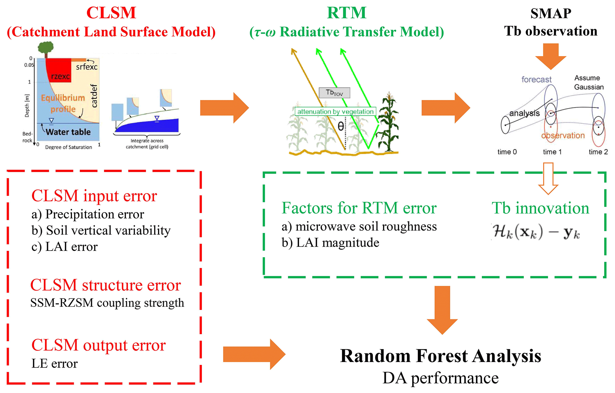
Figure 1 Systematic connection in the DA framework and the association between the eight selected factors in the analysis.

Therefore, to achieve the two major objectives, we first evaluate the performance of L4 SSM and RZSM estimates using 2474 sites in China with soil moisture profile measurements (generally acquired at subsurface depths between 10 and 50 cm) during the 2-year period of 2017 to 2018. Next, the in situ measurements are used to assess the DA skill improvement of the L4 system, which is defined as the skill difference between the L4 estimates and the OL baseline. Additionally, we apply a machine learning technique to quantify by how much the eight potential control factors drive the spatial variations in the efficiency of the L4 system. In this way, we seek to prioritize future enhancements to the L4 system.

2 Data and methods

In this section, we briefly describe the SMAP L4 soil moisture product (Sect. 2.1), the network of in situ soil moisture observations in China (Sect. 2.2), the above-mentioned control factors and ancillary data sources (Sect. 2.3), and the vertical coupling metric used in the skill assessment (Sect. 2.4). Next, we introduce the double instrumental variable (IV_d) method employed to determine the errors in control factors that cannot be determined using ground observations (Sect. 2.5). Finally, we describe the random forest (RF) regression method used to identify the main factor(s) (out of the eight control factors from both CLSM and RTM aspects) that affect the spatial variations in SMAP L4 DA skill improvement and L4 performance (Sect. 2.6).

2.1 SMAP L4 soil moisture product

The SMAP L4 soil moisture product (version 4; Reichle et al., 2019) is generated by assimilating the SMAP L1C Radiometer half-orbit 36 km Equal-Area Scalable Earth (EASE) Grid T_b observations (Version 4 SPL1CTB; Chan et al., 2016) into the CLSM. The SMAP T_b observations are assimilated at 3 h intervals using a spatially distributed, 24-member ensemble Kalman filter (Reichle et al., 2017b). The surface meteorological forcing data are from the global Goddard Earth Observing System (GEOS) Forward Processing atmospheric analysis (Lucchesi, 2013), with precipitation corrected using the daily, 0.5^∘, gauge-based Climate Prediction Center Unified (CPCU) product (Xie et al., 2007). The L4 product provides global, 9 km, 3-hourly surface (0–5 cm), and root-zone (0–100 cm) soil moisture estimates along with related land surface fields and analysis diagnostics. For the present study, we aggregate all soil moisture estimates to daily averaged (00:00 to 23:59 UTC) data. The OL baseline is a model-only, ensemble CLSM simulation without the assimilation of SMAP T_b observations but otherwise using the same configuration, including perturbations, as in the L4 system (Reichle et al., 2021).

The SMAP L4 assimilation system includes a zero-order τ–ω forward RTM (De Lannoy et al., 2013) that converts SSM and surface soil temperature into L-band brightness temperature estimates. Selected parameters of the L4 RTM, including the microwave soil roughness parameter h, vegetation structure parameter τ, and the microwave scattering albedo ω, are calibrated using multi-angular L-band brightness temperature observations from the Soil Moisture Ocean Salinity (SMOS) mission (De Lannoy et al., 2014a). The L4 RTM parameterizes microwave soil roughness as a function of SSM (De Lannoy et al., 2013; their Eq. B1). Here, we use this parameterization to compute the 2017–2018 daily averaged microwave soil roughness estimates as one potential indicator of DA skill improvement (Sect. 2.3). The necessary parameters are obtained from L4 Land Model Constants output collection (https://doi.org/10.5067/KGLC3UH4TMAQ; Reichle et al., 2018a). The L4 Analysis Update Data output collection includes RTM predictions of T_b and the assimilated SMAP T_b observations (https://doi.org/10.5067/60HB8VIP2T8W; Reichle et al., 2018b).

To avoid the impact of seasonality, we perform our analysis using anomaly time series, derived by subtracting a seasonally varying (daily) climatology from each raw time series. The climatology of a given time series is obtained by sampling the mean value of all soil moisture estimates that fall within a 31 d moving window centered on a particular day of year. Moreover, L4 estimates of LE, sensible heat flux (H), and the climatological LAI inputs to CLSM and the RTM are obtained from the L4 Geophysical Data output collection (https://doi.org/10.5067/KPJNN2GI1DQR; Reichle et al., 2018c). These datasets are also used to compute control factors to explain spatial variations in the DA skill improvement of the L4 system (Sect. 2.3).

2.2 Soil moisture validation data

In situ soil moisture measurements during 2017 and 2018 are collected from a national network of Chinese Automatic Soil Moisture Observation Stations (CASMOS) maintained by the Chinese Meteorological Administration (CMA; Han et al., 2017). In total, soil moisture measurements from 2474 separate stations across China, and covering different land use types, are collected. At each CASMOS site, frequency domain reflectometry-based instruments (DNZ1, DNZ2, and DNZ3) are used to record hourly volumetric soil moisture content within the following vertical depth ranges: 0–10, 10–20, 20–30, 30–40, and 40–50 cm below the surface. This instrumentation – DNZ1, DNZ2, and DNZ3 – is separately produced by Shanghai Changwang Meteorological Science and Technology Corporation (Shanghai, China), Henan Meteorological Science Research Institute and the 27th Institute of China National Electric Power Corporation (Zhengzhou, China), and China Huayun Technology Development Corporation (Beijing, China), respectively. From the above-mentioned instruments, the hourly estimates (at multiple depths) are then aggregated into daily values and linearly averaged (vertically) to produce 0–10 cm (SSM) and 0–50 cm (RZSM) in situ soil moisture measurements, which are subsequently used to validate the L4 and OL SSM (0–5 cm) and RZSM (0–100 cm) estimates. Note that Spearman's correlation rather than Pearson's correlation is used for L4 and OL validation because Pearson's correlation assumes linear consistency of the underlying variables and is more sensitive to outliers. By employing Spearman's rank correlation, we do not need to exclude soil moisture outliers and thus avoid introducing ad hoc thresholds that would define outliers. Nonetheless, we repeat the analysis based on Pearson's correlation (not shown) and find that the results are qualitatively consistent with the results using Spearman's correlation.

Ground observations within the same 9 km EASE grid were averaged for comparisons against the collocated 9 km L4 and OL soil moisture estimates. A total of 2287 individual 9 km EASE grid cells within China are included in the analysis. Among them, 92.35 % of grid cells contain one in situ site, 7.26 % contain two sites, seven grid cells contain three sites, and the remaining two grid cells contain four and five sites respectively. Figure 2 shows the number of in situ CASMOS sites within each 9 km EASE grid.

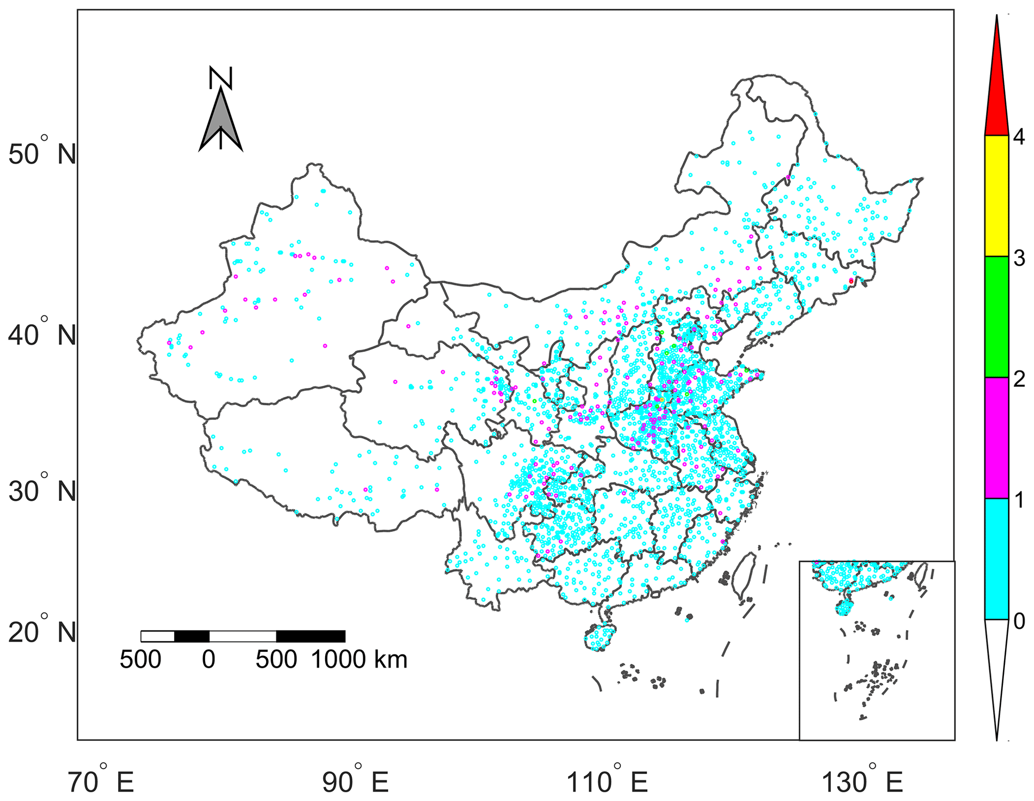
Figure 2 The number of in situ CASMOS sites within each 9 km EASE grid across the study area.

2.3 Explanatory data products

As discussed above, our hypothesis is that the efficiency of the SMAP L4 system will be sensitive to the ability of the ensemble-based L4 analysis in filtering errors that exist in CLSM, the RTM forecast T_b, and the assimilated SMAP T_b observations. We therefore consider two separate categories of factors that potentially control spatial variations in DA skill improvement. The factors are summarized in Table 1.

Table 1 Benchmark datasets and metrics used for evaluating control factors of SMAP L4.

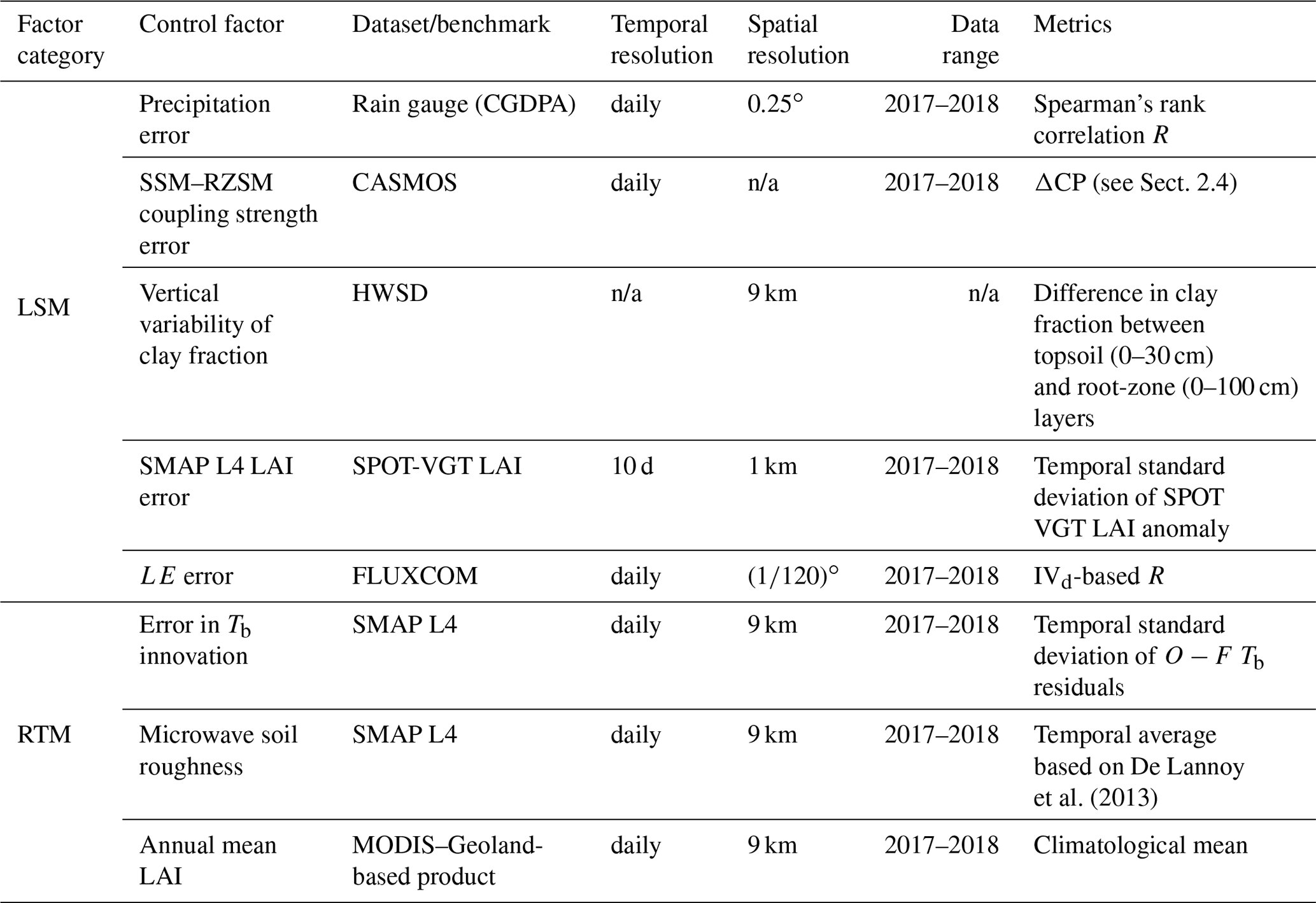
n/a stands for not applicable.

The first category represents a range of factors known to affect the skill of soil moisture estimates derived from the LSM (in this case, CLSM). The five control factors in this category are (1) the error in precipitation forcing, (2) the error in (input) LAI, (3) the error in (output) LE, (4) the magnitude of mean error in CLSM SSM–RZSM coupling strength, and (5) the presence of vertical variability in soil properties (defined as the difference in clay fraction across the vertical soil profile). Note that such variability represents a potential source of error because, with the exception of some surface-layer moisture transport parameters, CLSM assumes soil texture and associated soil parameters are vertically homogeneous within the soil column. However, the Harmonized World Soil Database (HWSD; FAO/IIASA/ISRIC/ISSCAS/JRC, 2012) often captures distinct vertical variations in soil properties, which are neglected by CLSM. Therefore the magnitude of vertical heterogeneity in soil texture may be an effective proxy for overall CLSM soil moisture accuracy. HWSD is selected due to its extensive use in soil science (De Lannoy et al., 2014b), and switching from HWSD to the high-resolution soil hydraulic and thermal properties dataset derived from the Global Soil Dataset for Earth System Models and SoilGrids (Dai et al., 2019) does not qualitatively change our conclusion or the importance ranking of vertical variability in soil properties (figure not shown). In addition, given the high specific surface area of clay and its high influence on soil structure and aggregation, the clay fraction is very important for soil moisture retention (Hillel, 1998), and thus the clay fraction is chosen over silt and sand fractions in the analysis. Besides, note that since LE and H are generally (strongly) anti-correlated, it is not appropriate to include both in a single random forest analysis – since including both would yield biased (high) regression weights for LE and H.

The second category contains three factors that affect radiative transfer modeling (RTM) and therefore DA updates. These include (1) estimates of the T_b innovation, namely the difference between SMAP T_b observations and RTM T_b simulations; (2) the magnitude of microwave soil roughness; and (3) the magnitude of LAI (as a proxy for the vegetation optical depth at microwave frequencies, which modulates the contribution of surface soil to the observed T_b).

The control factors take a variety of forms. Some factors are based on estimates of the errors fed into the L4 system, namely (1) the error in CLSM rainfall forcing data, (2) the error in SSM–RZSM coupling strength, (3) the vertical variability of clay fraction, (4) the SMAP L4 LAI error, (5) the output LE error, and (6) the error in T_b innovation. Other factors consist of the magnitude of the variable itself, namely the magnitude of microwave soil roughness and annual mean LAI. Note that LAI is used in both ways: LAI error is used to predict OL performance (because LAI is an important input into CLSM), while mean LAI is used to explain DA performance (because increased LAI is associated with decreased soil moisture information in microwave observations).

Note that the LAI used in the L4 system is a merged climatology from Moderate Resolution Imaging Spectroradiometer (MODIS) and Geoland data based on satellite observations of the normalized difference vegetation index (Mahanama et al., 2015; Reichle et al., 2017a). Therefore, to indicate the magnitude by which the LAI of each grid cell typically deviates from its long-term climatology, we use the temporal standard deviation for the anomaly time series of a benchmark LAI time series as a measure of the error in the LAI value used in the L4 system. This benchmark LAI is from the SPOT-VEGETATION (SPOT VGT) product and includes inter-annual variations (Sect. 2.3.3). Owing to the lack of reference T_b observations at similar satellite overpass times and locations, errors in T_b innovation are gauged using the time series standard deviation of the observation-minus-forecast (O−F) T_b residuals, which indicate the typical misfit between the RTM forecast T_b and the rescaled SMAP T_b observations. This rescaling process ensures zero-mean differences between T_b observations and forecasts and involves a seasonal multi-year-mean bias correction, which makes sure that the DA only corrects for errors in short-term and inter-annual variations and not for errors in the climatological seasonal cycles of the modeled soil moisture or other land surface fields. The standard deviation of the O−F T_b residuals measures the total error in T_b observation space.

The exact datasets and the metrics utilized for evaluating all eight control factors are summarized in Table 1.

2.3.1 Gauge-based precipitation gridded product

Errors in the precipitation data used to force the CLSM within the SMAP L4 system are estimated via Spearman's rank correlation with available rain gauge observations. These network observations are based on an analysis of ∼2400 rain gauge stations distributed across China (Shen and Xiong, 2015). Recently, the China Gauge-based Daily Precipitation Analysis (CGDPA) with a spatial resolution of $\mathrm{0.25}{}^{\circ }\times \mathrm{0.25}{}^{\circ }$ based on this network was constructed and has been made operational over China (http://data.cma.cn/data/cdcdetail/dataCode/SEVP_CLI_CHN_PRE_DAY_GRID_0.25.html, last access: 28 April 2020). CGDPA uses a modified version of climatology-based optimal interpolation (OI) with topographic correction proposed by Xie et al. (2007). In this process, the daily precipitation climatology over China is optimized and rebuilt using the 30-year average precipitation observations from ∼2400 gauges of the period 1971–2000 (Shen et al., 2010). CGDPA is shown to have smaller bias and root mean square error (for instance, 13.51 mm d⁻¹ vs. 17.02 mm d⁻¹ for precipitation of 25.0–50.0 mm d⁻¹) than the CPCU product used in the SMAP L4 system, which is based on fewer than 400 gauge sites over China (Shen and Xiong, 2015).

2.3.2 FLUXCOM LE estimates

The FLUXCOM ensemble of global land–atmosphere energy fluxes is used to evaluate error in L4 LE estimates. This ensemble merges energy flux measurements from FLUXNET eddy covariance towers with remote sensing and meteorological data based on four broad categories of machine learning method (namely tree-based methods, regression splines, neural networks, and kernel methods) to estimate global gridded net radiation, LE and H, and their related uncertainties (Jung et al., 2019). The resulting FLUXCOM database has a 0.0833^∘ spatial resolution when applied using MODIS remote sensing data. The monthly energy flux data of all ensemble members, as well as the ensemble estimates from the FLUXCOM initiative, are freely available (CC4.0 BY license) from the Data Portal, while the daily and 8 d FLUXCOM products are acquired from dataset provider Martin Jung (http://fluxcom.org/, last access: 16 April 2020). To calculate the LE error, we collected the daily, high spatial resolution FLUXCOM product and extracted the LE estimates where in situ soil moisture sites are located.

2.3.3 SPOT VGT LAI

The dataset used as a benchmark for assessing leaf area index (LAI) errors present in the SMAP L4 analysis is derived from the SPOT/VEGETATION and PROBA-V LAI products (version 2) that were generated every 10 d (at best) with a spatial resolution of 1 km. The SPOT LAI version 2 product GEOV2 is provided by the Copernicus Global Land Service (https://land.copernicus.eu/global/products/LAI, last access: 15 April 2020; Baret et al., 2013). It capitalizes on the development of already existing products: CYCLOPES version 3.1 and MODIS collection 5, based on neural networks (Baret et al., 2013; Verger et al., 2008). Compared to version 1, the version 2 products are derived from top of canopy daily reflectances, which ensures reduced sensitivity to missing observations and avoids the need for a bidirectional reflectance distribution function model.

2.3.4 HWSD soil texture

The soil texture information is from the HWSD attribute database (v1.2; FAO/IIASA/ISRIC/ISSCAS/JRC, 2012), which is a 30 arcsec raster database with 15 773 different soil-mapping units worldwide. It provides information on the standardized soil parameters for topsoil (0–30 cm) and subsoil (30–100 cm) separately. In this study, we use the difference of clay fractions between topsoil (0–30 cm) and the aggregated 0–100 cm layer to measure the vertical clay fraction variation at each 9 km grid cell.

2.4 Vertical coupling metric

The RZSM time series generally show decreased temporal dynamics relative to SSM. As a result, overestimated SSM–RZSM coupling tends to spuriously increase the (correlation-based) similarity of SSM and RZSM time series and, thereby, overestimate RZSM temporal variability. Therefore, analogous to the Kling–Gupta efficiency (Gupta et al., 2009), we define the SSM–RZSM coupling strength (CP) as

$$\begin{array}{}\text{(1)}& \mathrm{CP}=\mathrm{1}-\sqrt{(R-\mathrm{1}{)}^{\mathrm{2}}+(\mathit{\alpha }-\mathrm{1}{)}^{\mathrm{2}}},\end{array}$$

where R is Spearman's rank correlation between SSM and RZSM, and α is the ratio of temporal standard deviation of SSM to that of RZSM. The CP estimation is based on anomaly time series of both SSM and RZSM. A CP value of 1 represents the extreme case where RZSM is identical to SSM, i.e., a strongly coupled case. Likewise, a CP of 0 represents the opposing case of completely uncoupled time series. Cases with negative CP do not exist in this study.

Observed CP (CP_obs) was based on comparisons between 0–10 cm surface and 0–50 cm root-zone in situ observations and used as a benchmark. In contrast, CP estimates of OL (CP_OL) was based on the comparison of 0–5 cm surface and 0–100 cm root-zone estimates. Therefore, the surface versus root-zone storage contrast in the observation time series is less than that of the L4 estimates. This will likely cause the observed correlation between surface and root-zone time series to be systematically higher than the analogous vertical correlation calculation for L4 estimates. However, this bias is partially corrected for by the second term in Eq. (1) – since the observed α ratio will, by the same token, tend to be smaller (i.e. closer to 1) than α sampled from the L4 analysis. Such ability to compensate for vertical depth differences is a key reason we apply CP, rather than simple correlation, as a vertical coupling strength metric. Nevertheless, it should be noted that our main interest here lies in describing spatial variations in CP_OL–CP_obs, and care should be taken when interpreting raw CP_OL–CP_obs differences as an absolute measure of L4 vertical coupling bias.

2.5 Double instrumental variable (IV_d) method

The benchmark dataset of FLUXCOM LE described above contains error that is assumed to be of a similar order of magnitude as the L4 LE dataset it is applied to evaluate. Therefore, in an attempt to correct for the impact of this error, the LE error used here as a control factor is obtained via a double instrumental variable (IV_d; Dong et al., 2019b) analysis approach that minimizes the spurious impact of random errors in benchmark datasets. As shown in Dong et al. (2019b), for the evaluation of two time series containing autocorrelated errors, IV_d is more robust than a single instrumental-variable-based algorithm; therefore we apply IV_d to evaluate the LE error.

IV_d is a modified version of triple collocation (TC) analysis. In TC analysis (McColl et al., 2014), geophysical variables obtained from three independent sources (x_t, y_t, and z_t) at time t are assumed to be linearly related to the true signal P_t as

$$\begin{array}{}\text{(2)}& x_t={\mathit{\alpha }}_x{P}_t+B_x+{\mathit{\epsilon }}_{x,t},\end{array}$$

where the α_x is a scaling factor, B_x is a temporal constant bias, and ε_x,t is the zero-mean random error.

As opposed to the TC method, IV_d uses only two independent products (x, y) to characterize geophysical data product errors. This method introduces two instrumental variables I, which is the lag − 1 time series of x, and J, which is the lag − 1 time series of y, respectively.

$$\begin{array}{}\text{(3)}& {\displaystyle }& {\displaystyle }{I}_t={\mathit{\alpha }}_x{P}_{t-\mathrm{1}}+B_x+{\mathit{\epsilon }}_{x,t-\mathrm{1}}\text{(4)}& {\displaystyle }& {\displaystyle }{J}_t={\mathit{\alpha }}_y{P}_{t-\mathrm{1}}+B_y+{\mathit{\epsilon }}_{y,t-\mathrm{1}}\end{array}$$

Therefore, assuming that the errors of two independent products are serially white, the covariance between instrumental variables and products can be written as follows:

$$\begin{array}{}\text{(5)}& {\displaystyle }& {\displaystyle }{C}_{Ix}={\mathit{\alpha }}_x^{\mathrm{2}}{L}_{PP}\text{(6)}& {\displaystyle }& {\displaystyle }{C}_{Jy}={\mathit{\alpha }}_y^{\mathrm{2}}{L}_{PP},\end{array}$$

where C represents the covariance of the subscript products. For instance, C_Ix represents the covariance of x and its instrumental variable I. Variable L_PP is the lag − 1 auto-covariance of the true signal. Combining Eqs. (5) and (6), the scaling ratio $s_{{\mathrm{iv}}_{\mathrm{d}}}$ of the two products x and y can be written as

$$\begin{array}{}\text{(7)}& s_{{\mathrm{iv}}_{\mathrm{d}}}=\sqrt{{\displaystyle \frac{C_{Ix}}{C_{Jy}}}}.\end{array}$$

Based on Eq. (7), their correlation with truth can be estimated as

$$\begin{array}{}\text{(8)}& {\displaystyle }& {\displaystyle }{R}_{P_x}^{\mathrm{2}}={\displaystyle \frac{C_{xy}{s}_{{\mathrm{iv}}_{\mathrm{d}}}}{C_{xx}}}\text{(9)}& {\displaystyle }& {\displaystyle }{R}_{P_y}^{\mathrm{2}}={\displaystyle \frac{C_{xy}}{C_{yy}{s}_{{\mathrm{iv}}_{\mathrm{d}}}}}.\end{array}$$

In this way, the error in the L4 LE (measured by IV_d-based correlation with truth) can be estimated robustly using the FLUXCOM LE product described in Sect. 2.3.2.

2.6 Random forest regression

A random forest (RF) regression approach is used to quantify and rank the importance of the eight control factors introduced above (Table 1) for describing spatial patterns in DA skill improvement for both SSM and RZSM estimates. The RF method is a supervised learning algorithm based on an averaged ensemble of decision trees (Breiman, 2001). Unlike linear regression approaches, RF can capture nonlinear interactions between the features and the target. In addition, the normalization (or scaling) of data is not necessary in RF application. Another advantage of the RF algorithm is that it can readily measure the relative importance of each feature on the estimates, which makes it highly suitable for an attribution analysis. Therefore, based on the output of RF, key control factors determining the skill improvement of SMAP DA are evaluated and ranked. The RF estimates are based on a 10-fold cross-validation approach.

3 Results

3.1 Validation of SMAP L4 and OL estimates of SSM and RZSM anomalies

Figure 3 maps validation results (i.e., Spearman's rank correlation of anomaly with in situ observations, R) for SMAP L4 and associated OL soil moisture estimates. The skill patterns for OL and L4 are, in general, quite spatially consistent. Both are characterized by an increasing trend of SSM estimation skill moving from northwestern to southeastern China (Fig. 3a and b) that matches the increasing density of the rain gauge network. In relative terms, the L4 product surpasses the baseline OL's SSM skill for 77 % of the 2287 9 km EASE grid cells containing ground observations – with a mean R increase of ΔR=0.056 [–] and mean relative improvement versus R_OL of 14 %.

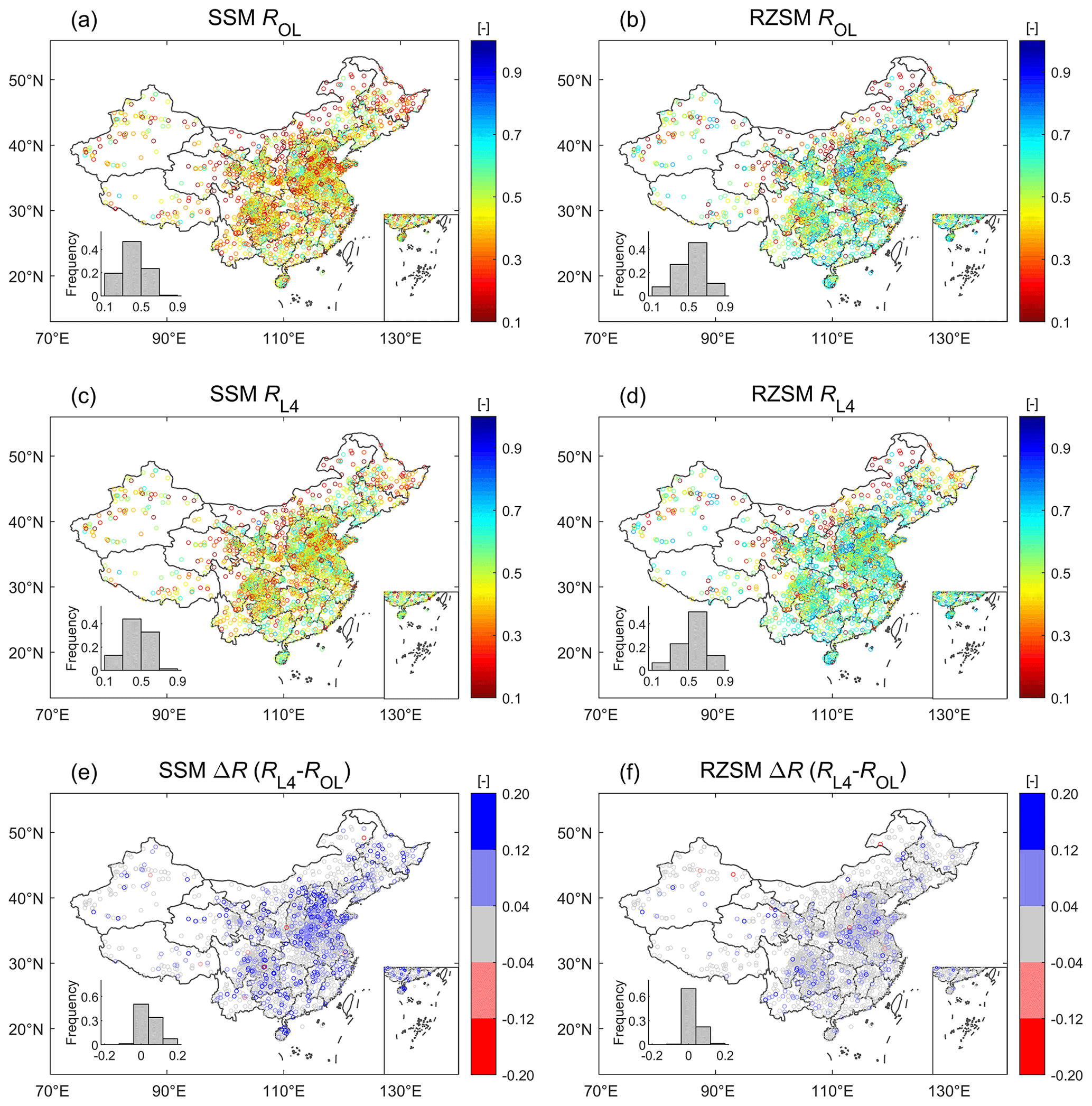
Figure 3 OL (a, b) and L4 (c, d) skills (R values) for SSM (a, c, e) and RZSM (b, d, f). DA skill improvement ($\mathrm{\Delta }R=R_{\mathrm{L}\mathrm{4}}-R_{\mathrm{OL}}$) for (e) SSM and (f) RZSM. Blue (red) colors in (e) and (f) indicate grid cells where L4 estimates are better (worse) than OL. Non-significant differences (based on a 1000-member bootstrapping analysis) are shaded grey. The lower left inset in each subplot indicates the frequency of binned R values across all 9 km EASE grid cells containing ground observations.

Similar spatial patterns are observed for RZSM skill. As with SSM, generally higher consistency with in situ RZSM measurements is found in southeastern China relative to northwestern China. However, relative to SSM, the benefit of SMAP data assimilation (i.e., L4) is reduced for RZSM, and the mean relative R improvement is only 7 % (ΔR=0.034 [–]) (compare Fig. 3e and f). This reduction is expected since assimilated SMAP T_bs are primarily sensitive to soil moisture conditions in the surface (0–5 cm) layer.

3.2 Spatial distribution of potential factors controlling SMAP L4 DA performance

As described in Sect. 2.3, we select eight control factors that potentially influence the skill of SMAP L4 soil moisture estimates. Using the attribution analysis described in Sect. 2.6, these factors are used to explain the spatial variations in DA skill and DA skill improvement seen in Fig. 3. As a first step, this section examines the spatial patterns inherent in the eight control factors. Errors in the CLSM precipitation forcing are relatively higher in northwestern China (Fig. 4a), where the gauge density is generally sparser than in southern China. Among the factors representing CLSM structural errors, a predominantly negative bias is observed in SSM–RZSM coupling strength generally across China (i.e., lower CP_OL compared to CP_obs), while a very small number of grid cells show a positive coupling strength bias in eastern China (dark green dots in Fig. 4b). This is expected since the coupling strength generally decreases with coarser resolution; i.e., the vertical coupling strength of the model is assumed much lower than that of any single site. In addition, this may be partially attributed to layer depth differences, since CLSM represents surface and root-zone depths of 0–5 and 0–100 cm, respectively, whereas the corresponding in situ observations represent the 0–10 and 0–50 cm layers. Therefore, CP_OL is likely to be systematically smaller than CP_obs. In addition, the vertical variability of the clay fraction seems to show little spatial variation across China (Fig. 4c). With respect to CLSM LAI error, regions in southern China that have generally higher LAI show larger standard deviations in SPOT LAI time series (Fig. 4d and h). The IV_d-based estimates of SMAP L4 LE error, which represent a potential control factor for water-balance errors in CLSM, generally show a low level of error across China (Fig. 4e).

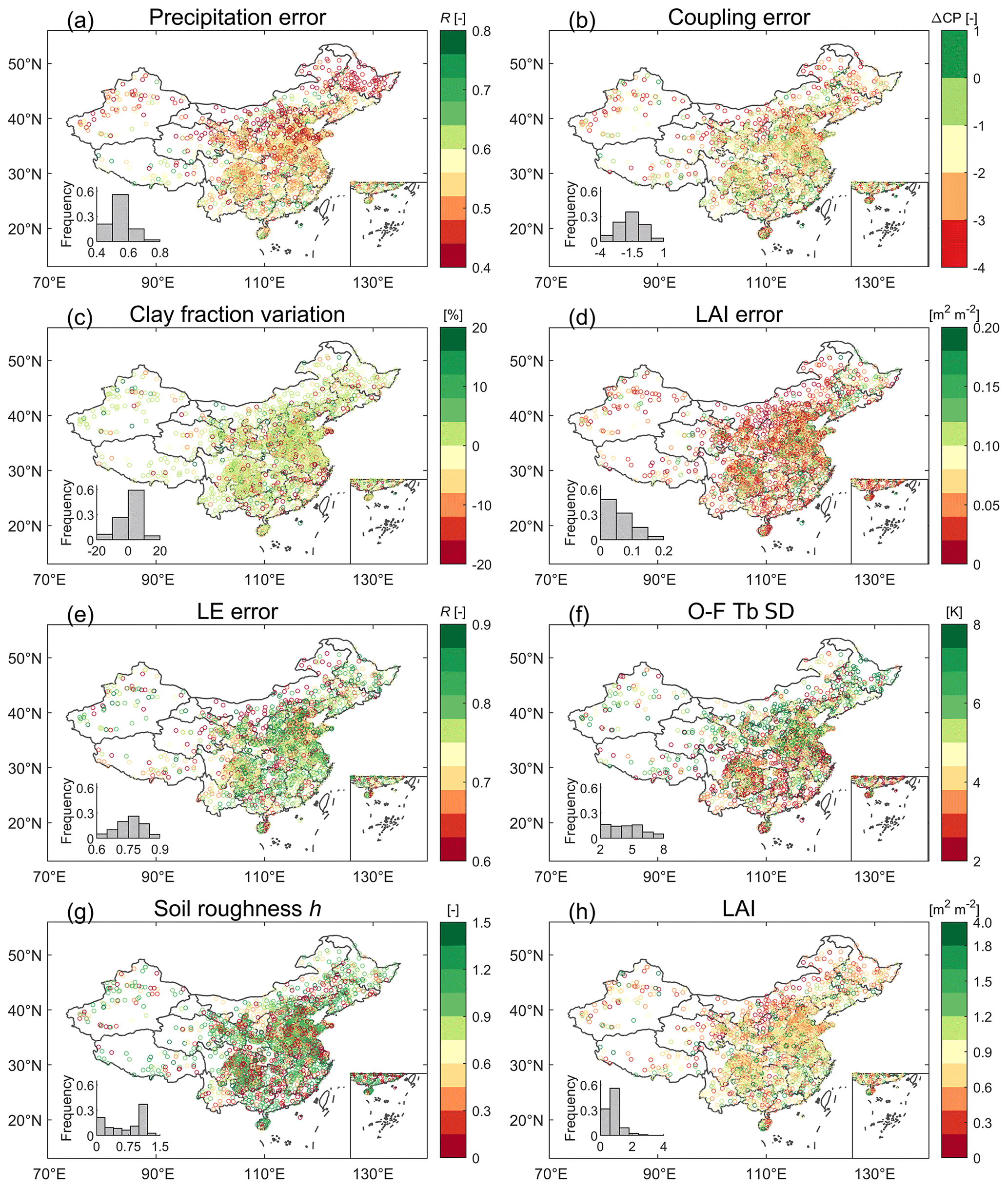
Figure 4 Factors potentially influencing SMAP L4 performance over the study area: (a) CLSM precipitation error measured by the Spearman's rank correlation between CLSM precipitation and ground observations; (b) SSM–RZSM coupling strength error (CP_OL minus CP_obs); (c) clay fraction variation (difference) across the soil profile; (d) error in LAI input to L4; (e) IV_d-based error of LE from L4; (f) O−F T_b standard deviation; (g) L4 microwave soil roughness; (h) climatology mean of LAI input to L4. The last row shows factors that consist of the magnitude of the variable itself, while the other rows show factors based on estimates of the errors that are fed into the L4 system.

Figure 5 Attribution analysis of SMAP L4 DA skill improvement: (a) cross-validation of RF regression method in predicting DA skill improvement $\mathrm{\Delta }R=R_{\mathrm{L}\mathrm{4}}-R_{\mathrm{OL}}$ based on our eight control factors (Table 1). Relative importance of eight control factors determining spatial patterns in (b) DA skill improvement (ΔR), (c) OL performance (R_OL), and (d) L4 performance (R_L4). Red (blue) bars represent predictor importance for SSM (RZSM). Error bars reflect the standard deviation from 50-member bootstrapping of the RF importance estimates. Since RTM-related errors do not impact the SM skill in the OL simulation, the corresponding bars in panel (c) are shown as semi-transparent (see text for details).

For O−F T_b residuals describing RTM-related error, a higher standard deviation of O−F T_b residuals is observed in the North China Plain (Fig. 4f), which is very consistent in spatial distribution with areas displaying the highest and most significant SSM prediction improvement (Fig. 3c). This is expected, as mentioned above, because O−F T_b residuals are the basis for the soil moisture corrections (or increments) that are applied in the DA system as part of the L4 analysis. The 2017–2018 mean of soil roughness shows a relatively scattered spatial pattern (Fig. 4g), while the 2017–2018 mean LAI shows higher values in southwestern and southeastern China (Fig. 4h).

3.3 Attribution of SMAP L4 versus OL performance to control factors

3.3.1 Attribution using random forest regression

As mentioned above, RF regression is used to identify the relative importance of our eight control factors for determining the improvement of SMAP L4 DA (i.e., $\mathrm{\Delta }R=R_{\mathrm{L}\mathrm{4}}-R_{\mathrm{OL}}$) and also R_L4 and R_OL. We first investigate the robustness of RF for predicting ΔR. To estimate the magnitude of randomness in the RF algorithm, we use 50 bootstrap runs. As shown in Fig. 5a, the 10-fold cross-validation test (228 validation samples) shows that the predicted and in situ-based ΔR have a mean correlation of 0.72 and 0.46 for SSM and RZSM, respectively. In Fig. 5a, the mean and median of the cross-validation correlation are shown by the black circle and black line respectively within the boxes, while the second and third quartiles of the cross-validation correlation are shown by the edges of boxes.

Given the sampling errors of ΔR, which is based on a 2-year validation period, and the relatively low spatial variability in RZSM skill (Fig. 2f), the performance of RF is acceptable. In addition, the upscaling error of the ground measurement is likely a significant contributor to unexplainable spatial variability for ΔR in Fig. 3. In fact, Chen et al. (2016) found large spatial variability in the ability of point-scale SSM ground observations to describe grid-cell-scale SSM dynamics. In situ sites associated with larger random point-to-grid upscaling errors will introduce a spurious low bias into sampled estimates of ΔR values (see Appendix B in Dong et al., 2020). Therefore, part of the ΔR spatial variability observed in Fig. 3 is unrelated to any aspect of the L4 system and, therefore, unexplainable via our eight selected control factors.

Independent representativeness errors have an equal impact on both the L4 and OL skill assessments and should therefore not bias the relative skill assessments of L4 versus OL, particularly when these assessments are based on averaging across multiple grid cells. This holds if the location of ground-based measurements sites (within a footprint) is purely random. For the systematic sampling errors, we analyze the site representativeness using the 500 m MODIS Land Cover product (MCD12Q1 v6) of 2017, using the IGBP dataset. First, we take the land cover (LC) type of the MODIS grid cell where a given in situ site is located as the ground-based LC type. Next, we search all the MODIS grid cells that fall within the SMAP 9 km EASE grid cell where this in situ site is located. The latter area consists of about $\mathrm{20}\times \mathrm{20}=\mathrm{400}$ MODIS grid cells. We calculate the fraction of these 400 MODIS grid cells that have the same LC type as the ground-based LC and define this fraction as the site representativeness. We find that 52 % of the 2474 sites have site representativeness higher than 50 %. When we use only these sites for the RF attribute analysis, the top three factors controlling skill improvement (R_L4−R_OL), L4 skill (R_L4), and OL skill (R_OL) are still the same, although the precipitation error becomes the top influencer for R_L4 (not shown).

Based on the RF results, the T_b innovation is quantified as the most prominent factor in determining DA skill improvement (i.e., $\mathrm{\Delta }R=R_{\mathrm{L}\mathrm{4}}-R_{\mathrm{OL}}$) – followed by precipitation error and microwave soil roughness (Fig. 5b). The RF-derived ranking of control-factor importance for RZSM is similar to that of SSM in that the same three factors are still the most explanatory. However, relative to SSM, the importance of T_b innovation for RZSM decreased dramatically from >30 % to ∼15 %. Other modeling error sources (e.g., the vertical variability of soil properties) have only very limited impacts on SMAP DA improvement.

As seen in Fig. 5c, for the OL performance (R_OL), the most important factors identified by RF include precipitation error, SSM–RZSM coupling error, and T_b innovation (microwave soil roughness) for SSM (RZSM). Note that although the T_b innovation is identified as the third most important factor for R_OL in SSM skill, this is an instance where correlation does not imply a causal relationship (i.e., poorer skill happens to coincide with higher Tb innovation). Specifically, it is expected that T_b innovations are higher in areas where the OL performs worse, but a high T_b innovation is not the cause of a low OL performance. The same argument applies to the relationship between microwave soil roughness and OL skill for RZSM estimation. To retain the consistency with the analysis of R_L4 and avoid the misconnection between RTM-related factors and R_OL, the bars representing the importance of RTM-related factors to R_OL are shown as semi-transparent in Fig. 5c. The SMAP L4 system is able to reduce impact of precipitation errors on both SSM and RZSM estimation skill, rendering SSM–RZSM coupling error the most important factor for R_L4 (Fig. 5d). In addition, in the L4 system, the high vegetation density effect on SSM and RZSM estimation is clearly reduced, as the fourth most important factor of LAI magnitude is replaced by T_b innovation.

The qualitative rankings provided by the RF analysis in Fig. 5 are relatively robust to our particular choice of the benchmark dataset to define the “error” of various control variables. For instance, we replace the CGDPA precipitation benchmark with the Climate Prediction Center Morphing (CMORPH) merged product (Version 1, https://doi.org/10.25921/w9va-q159; Xie et al., 2019), which is the 0.1^∘ merging product of CMORPH and observations from more than 30 000 automatic weather stations in China. In this case, the predictive power of the regression model established by the RF is not affected (similar to Fig. 5a), and the qualitative rankings of the precipitation error in R_OL and R_L4 are not impacted (similar to Fig. 5c and d).

3.3.2 Attribution using box plot comparisons

As stated in Sect. 2.6, the RF method is adept at summarizing the impact of multiple (co-varying) control factors simultaneously in the established regression model and thus provides more comprehensive insights than the examination of how the target variable (DA improvement) fluctuates with each individual control factor. However, it does not allow for the investigation of the sign of the relationship between DA improvement and each control factor – which is important for understanding how each factor influences the DA system. In addition, since the net impact of various factors can enhance DA skill improvement by either degrading the OL or enhancing the ability of DA to add more value, it is important to decompose the source of variations in ΔR. Therefore, in addition to examining how SMAP DA skill improvement, i.e., $\mathrm{\Delta }R=R_{\mathrm{L}\mathrm{4}}-R_{\mathrm{OL}}$, varies as a function of the most prominent control factors identified above in Sect. 3.3.1 (i.e., T_b innovation, precipitation forcing error, and microwave soil roughness), we also examine how precipitation error as a control factor affects the OL performance, i.e., R_OL.

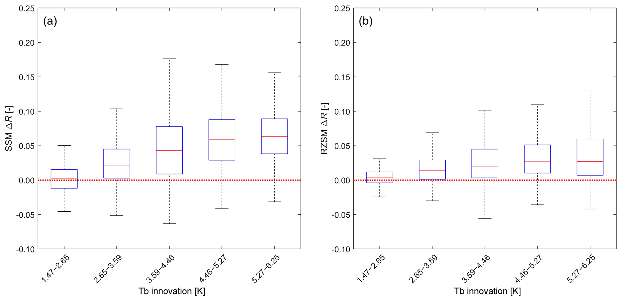
Figure 6 SMAP L4 DA skill improvement ($\mathrm{\Delta }R=R_{\mathrm{L}\mathrm{4}}-R_{\mathrm{OL}}$) as a function of T_b innovation for (a) SSM and (b) RZSM. Samples with T_b innovation ranking above the 80th percentile are excluded from the analysis.

To minimize the uncertainty caused by large errors in each of the control factors, we exclude samples with errors (separately for each control factor) ranking above the 80th percentile in the following analysis. The relationship between T_b innovations and L4 DA skill improvement is straightforward: higher T_b innovations are associated with higher ΔR, with ΔR generally larger for SSM than for RZSM (Fig. 6a and b).

For precipitation, this decomposition is illustrated in Fig. 7. Note that, as expected, low-quality precipitation tends to degrade the skill (i.e., correlation versus ground observations) of OL SSM and RZSM estimates (see Fig. 7a and b). This degradation provides an enhanced opportunity for SMAP L4 DA to provide benefit. As a result, ΔR tends to be an inversely proportional function of precipitation skill (i.e., higher precipitation skill leads to lower ΔR; see Fig. 7c and d). This inverse relationship is a well-known tendency for land DA systems (Liu et al., 2011; Bolten and Crow, 2012; Dong et al., 2019a). Precipitation quality has a diminished impact on RZSM estimation skill compared to SSM estimation skill. This is expected since RZSM is (essentially) the result of applying a low-pass time series filter to precipitation. As such, it is less sensitive to high-frequency errors in precipitation products than SSM is.

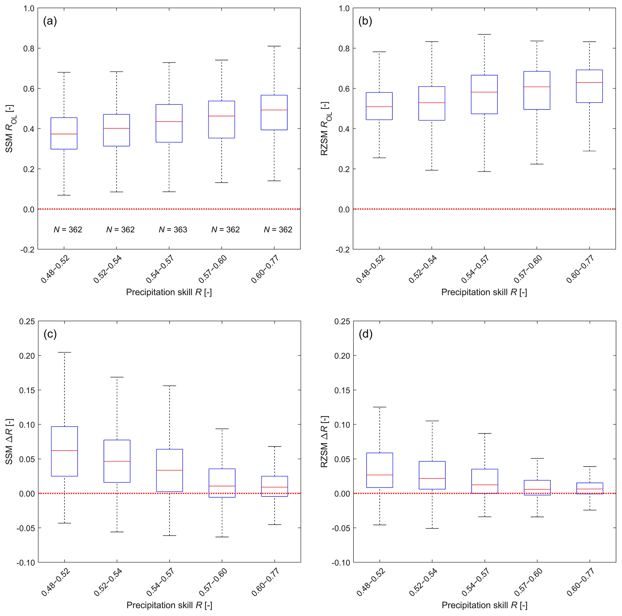
Figure 7 OL performance (R_OL) as a function of precipitation forcing skill R for (a) SSM and (b) RZSM. SMAP L4 DA skill improvement ($\mathrm{\Delta }R=R_{\mathrm{L}\mathrm{4}}-R_{\mathrm{OL}}$) as a function of precipitation skill for (c) SSM and (d) RZSM. Samples with precipitation skill ranking below the 20th percentile are excluded from the analysis.

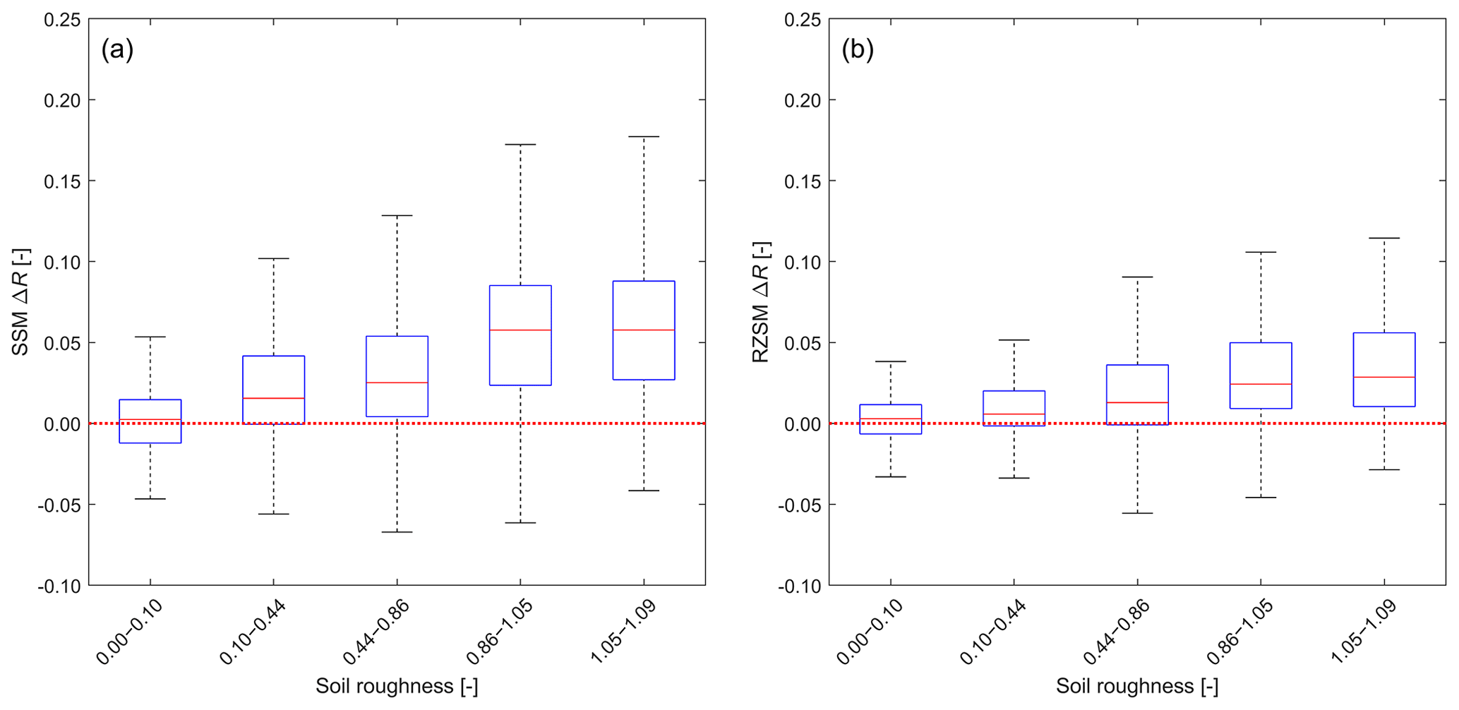
Figure 8 is analogous to Fig. 6 but shows skill differences ΔR as a function of microwave soil roughness. Similar to T_b innovations, it is as expected that this control factor has little impact on the OL performance, except that R_OL shows slight decreasing tendency with increasing soil roughness (not shown). Given the fact that the OL does get worse with increasing roughness, there is more room for improvement in areas with higher soil roughness, which makes it plausible that ΔR increases with increasing soil roughness (see Fig. 8a and b).

Figure 8 As in Fig. 6 but for ΔR as a function of microwave soil roughness.

Besides the above three control factors that dominate the DA skill improvement, we also examine the top factor that affects SMAP L4 performance, i.e., vertical coupling errors (Fig. 9). As expected, larger (absolute) bias in SSM–RZSM coupling in CLSM tends to be associated with degraded OL estimates of both SSM and RZSM (see Fig. 9a and b), although the analysis does not prove such a causal relationship. Similar to precipitation errors above, decreased OL skill (seen on the left-hand side of the figure panels) provides an opportunity for increased DA skill improvement – which is clearly seen in Fig. 9c and d. However, such increases are much larger for SSM than for RZSM.

For RZSM, SSM–RZSM coupling bias exerts both positive and negative effects on estimation accuracy. While such bias leads to an enhanced opportunity to improve upon a degraded OL, it should also hamper the ability of DA to transfer SSM increments into the root zone – particularly when, like here, the bias reflects the lack of vertical coupling in the model (Kumar et al., 2009). This means that some of the opportunity presented by the larger RZSM errors in OL is squandered by sub-optimal DA. As a result, the increase in RZSM DA skill improvement associated with biased SSM–RZSM coupling (Fig. 9d) is smaller than the analogous increase in SSM DA skill improvement (Fig. 9c).

Figure 9 As in Fig. 7 but for R_OL and ΔR as a function of SSM–RZSM coupling error indicated by the CP difference ($\mathrm{\Delta }\mathrm{CP}={\mathrm{CP}}_{\mathrm{OL}}-{\mathrm{CP}}_{\mathrm{obs}}$).

For the three strongest control factors that determine DA skill improvement ΔR, i.e., T_b innovation, precipitation error, and microwave soil roughness, we further conducted paired one-way analysis of variance. Results indicates that for each of the five binned groups separated by each of the above-mentioned three control factors, the inter-group difference in ΔR caused by each control factor is significant (p<0.01) for both SSM and RZSM. In addition, except for the groups with lowest mean ΔR in Figs. 6a and 8a, the averages of ΔR from all groups are significantly higher than 0 (p<0.01).

4 Conclusions

The SMAP L4 algorithm assimilates L-band T_b observations into the CLSM to provide surface and root-zone soil moisture estimates (i.e., SSM, RZSM) with 3-hourly, global coverage at 9 km resolution. The performance of the L4 soil moisture estimates compared to a baseline model-only simulation (OL) is influenced by multiple control factors associated with CLSM and the τ–ω RTM components of the L4 system. In this study, we assess the performance of the SMAP L4 DA system using 2 years of in situ soil moisture profile observations at 2474 sites across China. We apply a RF regression to identify the dominant factors (from a predefined list) that control the spatial distribution of the DA skill improvement (defined as the skill difference between the L4 and OL estimates of SSM and RZSM as measured by their Spearman rank correlation with in situ measurements). Results show that L4 improves SSM prediction skill by 14 % on average, with over 77 % of the 2287 9 km EASE grid cells showing an increase in Spearman's rank correlation with in situ observations. Similarly, widespread, though smaller, improvements are observed in RZSM, with average R improvement of 7 %.

Based on the RF regression analysis, the benefit of SMAP L4 DA for SSM is primarily determined by T_b innovation (measured by standard deviation of O−F T_b residuals), followed by microwave soil roughness and daily precipitation error. These three factors are also the most prominent factors controlling SMAP DA improvement for RZSM, albeit with the T_b innovation being the least important of these three factors for RZSM DA skill improvement.

Generally, the OL performance clearly decreases with increasing precipitation error, whereas for L4 performance precipitation error is not identified as the most dominant control factor. This indicates that the L4 system is able to correct for errors in precipitation forcing. In addition, our results demonstrate that SMAP DA contributes the most benefit for cases where CLSM underestimates SSM–RZSM vertical coupling strength. However, due to the difference in top-layer soil depth between the in situ observations (10 cm) and the L4 analysis (5 cm), it is unclear whether or not the observed SSM–RZSM coupling strength biases are real in an absolute sense – or simply reflect inconsistencies in the depth of modeled versus observed SSM and RZSM time series. Nevertheless, it is worth stressing that, despite the ambiguity about their absolute magnitude/sign, relative variations in apparent SSM–RZSM coupling biases explain a significant amount of the observed spatial variation in L4 performance. Therefore, this finding clearly underpins the importance of properly specifying SSM–RZSM coupling strength in CLSM as a way to improve the SMAP L4 product.

For SMAP L4 SSM skill, the next most important factors (after SSM–RZSM coupling) are the precipitation error, the T_b innovation, and microwave soil roughness (Fig. 5d). For L4 RZSM skill, the next most important factors (after SSM–RZSM coupling) are the precipitation error, the T_b innovation error, and the LE error, with the latter two factors of comparable importance (Fig. 5d). To enhance the L4 performance, additional focus should thus be placed on improving the model's characterization of the microwave radiative transfer modeling (T_b innovation), together with the partitioning of the available energy into latent and sensible heat (LE error).

Some of our RF analysis results fall squarely within expectation; for instance, the OL skill is predominately determined by precipitation error, which is in line with the previous studies using core validation site, sparse network sites, and other microwave soil moisture datasets (Reichle et al., 2017a, 2021; Dong et al., 2019a), and L4 skill improvement (i.e., R_L4−R_OL) is mostly determined by T_b innovation. On the other hand, there are also some more surprising results. For instance, we found that SSM–RZSM coupling error and precipitation error have a comparable impact on OL. For L4 skill, however, the impact of SSM–RZSM coupling error exceeds that of precipitation error. More specifically, L4 DA contributes the most benefit for cases where CLSM underestimates SSM–RZSM vertical coupling strength. This is the first quantification of the impact of different DA aspects (including background model structure error and model input error) on DA performance. These findings could be used for L4 product development. In addition, this study pinpoints that the L4 skill improvement is not heavily impacted by LAI magnitude, which gives confidence for using the L4 product over densely vegetated areas.