Implications of model selection: a comparison of publicly available, conterminous US-extent hydrologic component estimates

Spatiotemporally continuous estimates of the hydrologic cycle are often generated through hydrologic modeling, reanalysis, or remote sensing (RS) methods and are commonly applied as a supplement to, or a substitute for, in situ measurements when observational data are sparse or unavailable. This study compares estimates of precipitation (P), actual evapotranspiration (ET), runoff (R), snow water equivalent (SWE), and soil moisture (SM) from 87 unique data sets generated by 47 hydrologic models, reanalysis data sets, and remote sensing products across the conterminous United States (CONUS). Uncertainty between hydrologic component estimates was shown to be high in the western CONUS, with median uncertainty (measured as the coefficient of variation) ranging from 11 % to 21 % for P, 14 % to 26 % for ET, 28 % to 82 % for R, 76 % to 84 % for SWE, and 36 % to 96 % for SM. Uncertainty between estimates was lower in the eastern CONUS, with medians ranging from 5 % to 14 % for P, 13 % to 22 % for ET, 28 % to 82 % for R, 53 % to 63 % for SWE, and 42 % to 83 % for SM. Interannual trends in estimates from 1982 to 2010 show common disagreement in R, SWE, and SM. Correlating fluxes and stores against remote-sensing-derived products show poor overall correlation in the western CONUS for ET and SM estimates. Study results show that disagreement between estimates can be substantial, sometimes exceeding the magnitude of the measurements themselves. The authors conclude that multimodel ensembles are not only useful but are in fact a necessity for accurately representing uncertainty in research results. Spatial biases of model disagreement values in the western United States show that targeted research efforts in arid and semiarid water-limited regions are warranted, with the greatest emphasis on storage and runoff components, to better describe complexities of the terrestrial hydrologic system and reconcile model disagreement.

1 Introduction

A long-term goal of the atmospheric and hydrologic scientific communities has been to produce accurate estimates of the hydrologic cycle across continental and global domains (Archfield et al., 2015; Beven, 2006; Freeze and Harlan, 1969). Various methodologies have been applied to meet this goal, typically in the form of physically based, reanalysis, or remote-sensing-based models. Many of the resulting estimates are made publicly available by an assortment of scientific entities at both continental and global extents across a wide range of spatiotemporal resolutions. These data sets accelerate progress in the atmospheric and hydrologic sciences by filling knowledge gaps in data-sparse regions, reducing the need for time-consuming and computationally expensive modeling, and by providing numerous estimates to apply within ensemble analyses.

Publicly available modeled estimates have been applied to work on water budget analyses (Gao et al., 2010; Pan et al., 2012; Rodell et al., 2015; Smith and Kummerow, 2013; Velpuri et al., 2019; Zhang et al., 2018), the effects of climate change (La Fontaine et al., 2015; G. J. McCabe et al., 2017), and water availability and use (Landerer and Swenson, 2012; Thomas and Famiglietti, 2019; Voss et al., 2013; Zaussinger et al., 2019). Rapid increases in computational power and data accessibility following the advent of early global- and continental-extent hydrologic models in the 1980s and 1990s (Koster and Suarez, 1992; Manabe, 1969; Sellers et al., 1986; Yang and Dickinson, 1996), and increasingly higher-resolution passive and active satellite measurements of both the surface and subsurface of the Earth (Alsdorf et al., 2007; M. F. McCabe et al., 2017), have led to an explosion in the production of multidecadal, continental- to global-extent models estimating all major components of the hydrologic cycle (Peters-Lidard et al., 2018). Accordingly, this has given rise to a multitude of model comparison and evaluation projects throughout the scientific literature.

Earlier model intercomparison projects, such as the Coupled Model Intercomparison Project (CMIP; Covey et al., 2003), the Integrated Hydrologic Model Intercomparison Project (IH-MIP; Kollet et al., 2017; Maxwell et al., 2014), the Agricultural Model Intercomparison and Improvement Project (AgMIP; Rosenzweig et al., 2013), and the Water Model Intercomparison Project (WaterMIP; Haddeland et al., 2011), provide robust analyses aimed at attributing differences in model process representation to differences in model design, parameter selection, and meteorological forcings.

Detailed comparisons between smaller selections of models are often included in studies presenting novel products (Daly et al., 2008; Senay et al., 2011; Velpuri et al., 2013; Xia et al., 2012a, b). Furthermore, a range of studies have focused solely on the validation of third-party models, either examining multiple water budget components simultaneously (Gao et al., 2010; Sheffield et al., 2009) or focusing on specific components such as precipitation (P; Derin and Yilmaz, 2014; Donat et al., 2014; Guirguis and Avissar, 2008; Prat and Nelson, 2015; Sun et al., 2018), evapotranspiration (ET; Carter et al., 2018; McCabe et al., 2016), snow water equivalent (SWE; Broxton et al., 2016; Chen et al., 2014; Dawson et al., 2016, 2018; Essery et al., 2009; Mudryk et al., 2015; Rutter et al., 2009; Vuyovich et al., 2014), or soil moisture (SM; Brocca et al., 2011; Koster et al., 2009; Xia et al., 2014).

Most of these comparison studies have revolved around error metrics derived through validation against in situ and ex situ measurements. However, validation often yields unsatisfactory representations of model skill. Observational data sets are often spatiotemporally discontinuous, and model estimates in grid structure may not sufficiently represent the sub-grid heterogeneity that is present in point data, especially in topographically and ecologically complex regions. Furthermore, observational measurements can have significant associated uncertainty (Di Baldassarre and Montanari, 2009). Validation literature is heavily focused on the comparison of error statistics and spatial summaries of model skill and rarely discusses the effect of model disagreement on research results.

This research seeks to supplement past comparison and validation literature by evaluating how uncertainty between publicly available water budget component estimates used within a study can control outcomes and conclusions across a range of ecological regimes. We differentiate this work from previous model intercomparison and validation studies by placing results in the context of multiple water budget analyses. We seek to quantify how estimates of component magnitudes and long-term trends differ in the conterminous United States (CONUS) and within ecologically distinct regions. The primary goal of this work is to quantify model disagreement in terms of magnitude, interannual trend, and correlation against remote sensing (RS) products. The effects of model disagreement are shown in regional water budget analyses. We undertake a robust comparison of P, ET, R, SWE, and SM estimates generated through hydrologic models, reanalysis data sets, and remote sensing products. We iteratively calculate water budget imbalances in eight regions by applying a range of flux estimates to quantify how model selection may impact residuals.

2 Methods and data

2.1 Data categories

Hydrologic estimates are divided into water budget flux components of P, ET, and R, and storage components of SWE and SM, representing the primary fluxes and stores of a surface water budget. Data sets were selected by prioritizing public availability, ease of access, and relative use within the research community. These data sets are subdivided into loosely defined categories of hydrologic models, reanalysis data sets, and remote-sensing-derived products. References and spatiotemporal information for each data set are provided in Table 1, and more detailed long-form descriptions are provided in Appendix A.

Table 1 Summary of data sets used in this research, including assigned data category, abbreviated name, primary organization, literature reference, spatiotemporal resolution, and sourced hydrologic components. The reader is referred to Appendix A for definitions of abbreviated model names, descriptions, and further references. Components are precipitation (P), evapotranspiration (ET), runoff (R), snow water equivalent (SWE), and soil moisture in equivalent water depth and volumetric water content (SM(e) and SM(v), respectively). Hydrologic models NMH-MWBM and NMH-PRMS are based on a delineated (i.e., non-gridded), topographically derived spatial framework composed on hydrologic response units (HRUs). The reanalysis product WaterWatch is generated at hydrologic units (HUs) 2–8. The finest-resolution product, HU8, is used in this study.

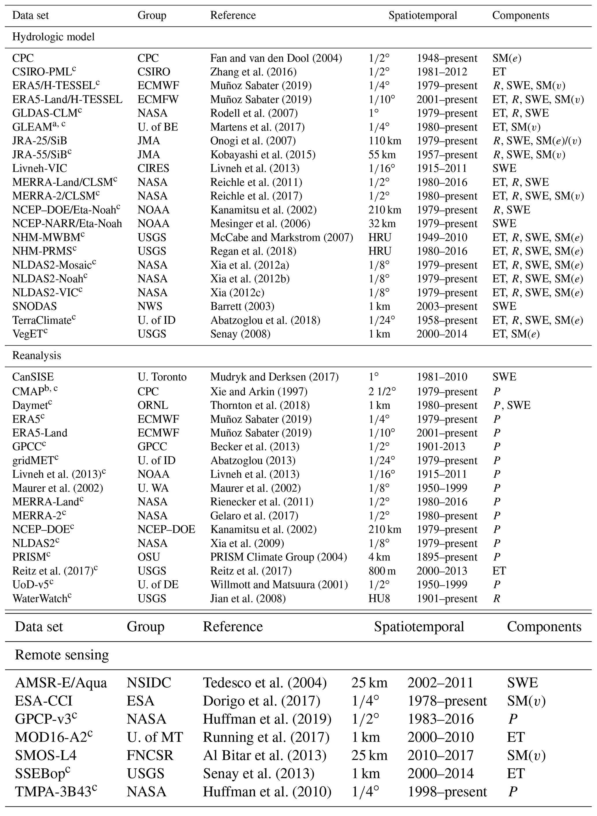
^a Versions 3.3a and 3.3b. ^b Standard and enhanced versions. ^c Data sets used in the water budget case study with complete data for water years 2001–2010.

2.1.1 Hydrologic models

The hydrologic model category (Table 1; Appendix A) includes any estimates generated using equations or concepts attempting to represent real-world hydrology. Model output differences are strongly controlled by forcing data sets (Elsner et al., 2014; Mizukami et al., 2014), calibration methods (Mendoza et al., 2015), applied equations (Clark et al., 2015a), model structure (Clark et al., 2015a, b), and geophysical parameter availability (Beven, 2002; Bierkens, 2015; Mizukami et al., 2017). The most common hydrologic models this study evaluates are conceptual and physically based. Conceptual models derive terrestrial hydrology estimates through empirical relationships between fluxes and stores, typically through a water balance model (WBM) in the style of Thornthwaite (1948; NHM-MWBM and TerraClimate). Physically based models utilize meteorological forcing data and solve equations describing physical conservation laws of mass, energy, and momentum. These can be further sub-divided by targeted hydrologic variables as follows: land surface models (LSMs) target land–atmosphere interactions, especially ET, while catchment models (CMs) target streamflow (Archfield et al., 2015). Additionally, LSMs are often 1D models that operate at discrete spatial intervals, typically grid cells, lacking horizontal transfer of surface or subsurface water between regions. CMs, on the other hand, utilize 2D model structures by routing overland and subsurface flows between spatial domains to better realize surface and groundwater estimates using prescribed stream networks. The CLSM, described in the literature as a land surface model (Koster et al., 2000), is discussed in conjunction with the NHM-PRMS because of the sub-grid catchment network used to model horizontal runoff and streamflow fluxes. LSMs are the most common hydrologic model here (e.g., CLM, H-TESSEL, Mosaic, Noah, SiB, and VIC) because they are often coupled with global-extent atmospheric research and, thus, more commonly operated at the spatial extent of this study, while CMs are more typically operated at the catchment or basin scale. Additional products included in the hydrologic model category are those using simplified WBMs falling outside the conceptual model paradigm (CPC, CSIRO-PML, GLEAM, and VegET) and those using component-specific physically based models (SNODAS).

2.1.2 Reanalysis

Reanalysis data sets (Table 1; Appendix A) assimilate multisource in situ and ex situ observational data into spatiotemporally continuous 4D estimates of continental- or global-scale atmospheric and meteorological fluxes using numerical algorithms. This category includes reanalysis data sets derived solely from in situ and ex situ data (e.g., CMAP, Daymet, Maurer et al., 2002, and UoD-v5) and those assimilating or blending multiple reanalysis products with or without observational measurements (e.g., CanSISE, gridMET, Livneh et al., 2013, and NLDAS2). In past studies, reanalysis models were often grouped and defined separately from gridded data sets derived through statistical interpolation of in situ observations (e.g., WaterWatch, Reitz et al., 2017, and GPCC). We combine the two categories, defining the single reanalysis category as containing products not generated solely from remote sensing observations or through terrestrial hydrologic models. The reasons for this are two-fold, i.e., (1) to simplify reporting of results and discussion across water budget components, and (2) although interpolation-based products are often used as reference data sets in model validation studies, especially for precipitation, accuracy decreases in regions with sparse observations and complex topography (Hofstra et al., 2008) and, thus, should be considered modeled products.

2.1.3 Remote sensing derived

The RS-derived data sets (Table 1; Appendix A) are components of the hydrologic system derived from passive and/or active ex situ observations. We note the use of the term RS-derived rather than RS because none of the data sets used here can be truly described as direct observations as they are always relying on a range of modeling techniques to create hydrologic estimates. For example, the AMSR-E/Aqua SWE product uses a sequence of steps including a snow-detection routine, followed by a physical retrieval algorithm, which is then validated against observational SWE data (Chang and Rango, 2000), and the SSEBop product uses a radiation-driven energy balance model to estimate ET (Senay et al., 2013). Remote sensing data sets include estimates modeled from single-sensor ex situ observations (MOD16-A2 and SSEBop), though most utilize an assembly of information from both passive and active sensors at various spatiotemporal resolutions (e.g., ESA-CCI and GPCP-v3).

2.2 Data processing

Data sets included in this research cover a broad spectrum of spatial resolutions, extents, coordinate reference systems, and timescales and, therefore, require a uniform spatiotemporal system to better facilitate comparison. To that end, gridded (e.g., NLDAS2-Mosaic) and polygonal (e.g., NHM-PRMS) data sets were aggregated by area-weighted mean to 10 Environmental Protection Agency Ecoregions, Level I (Omernik and Griffith, 2014), that encompass the Watershed Boundary Dataset hydrologic units (U.S. Geological Survey, 2016; Fig. 1; Table 2) over the CONUS. Data sets were processed in their native coordinate system to avoid interpolation of raw values, and the reference system of the ecoregions' spatial data set was transformed to match that of each target data set. Flux and storage terms were aggregated to monthly time steps. Flux values (P, ET, and R) were summed from hourly or daily when necessary, and storage values (SWE and SM) were averaged.

Table 2 Sizes of study ecoregions in square kilometers (km²) and percent (%) of study domain.

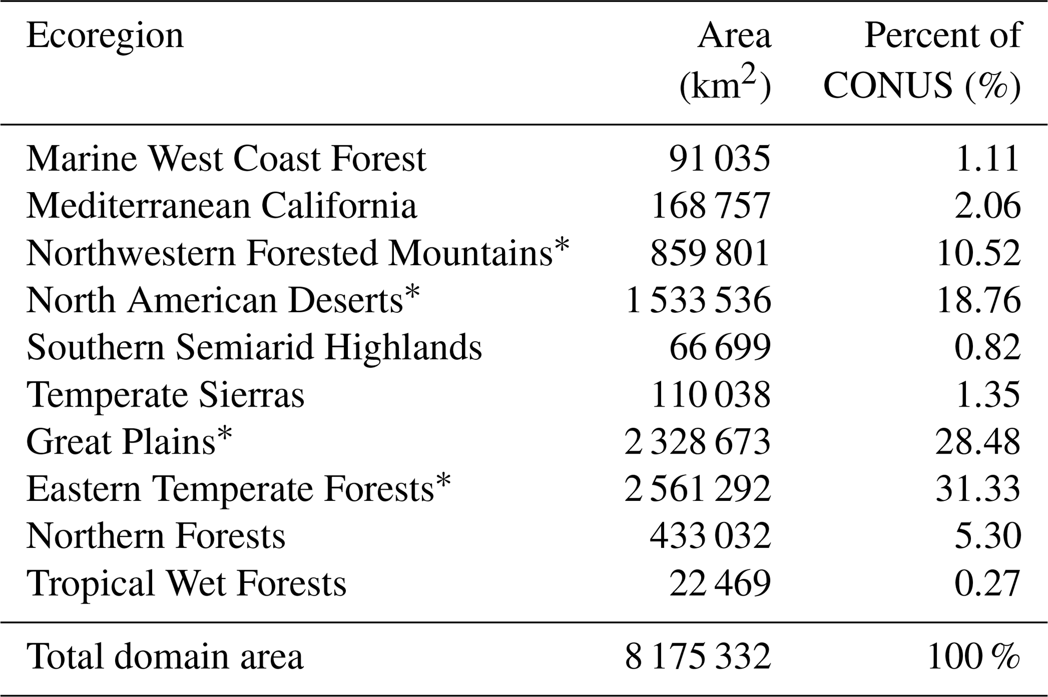
^* Primary ecoregions highlighted during water budget analysis.

Units of P, ET, R, and SWE are uniformly presented as equivalent water depth in millimeters (mm). SM is provided by data sets as either equivalent water depth (mm) or volumetric soil moisture content (m³ per cubic meter) and denoted as SM(e) or SM(v), respectively. The SM(e) and SM(v) categories are merged during results and discussion when magnitude is irrelevant, such as with long-term trend and correlation against RS products. All data generated through these methods are available in an associated data release hosted on the USGS ScienceBase (Saxe et al., 2020).

Figure 1 Distribution of the 10 ecoregions covering the CONUS study domain.

2.3 Statistics

2.3.1 Annual uncertainty

Uncertainties in hydrologic component values are measured as the variability between modeled estimates using the coefficient of variation (CV) calculated as follows:

$$\begin{array}{}\text{(1)}& \mathrm{CV}={\displaystyle \frac{\mathit{\sigma }}{\stackrel{\mathrm{‾}}{x}}}\times \mathrm{100}\mathit{\%},\end{array}$$

where σ is the standard deviation across all products of a given component in a given water year, and $\stackrel{\mathrm{‾}}{x}$ is the associated mean. The σ and CV statistics were calculated for each water year (WY; a water year is the 12 month period of 1 October through 30 September and is designated by the calendar year in which it ends) between available estimates for all components. Annual values of flux terms (P, ET, and R) were derived by summing monthly values to WYs, and storage terms were derived by averaging monthly values by WY. Incomplete WYs (n months <12) were discarded. Because of incompatibility between data set temporal ranges, σ and CV values were divided into two 15 WY periods, namely the early period consisting of WYs 1985–1999 and the late period consisting of WYs 2000–2014.

Uncertainty metrics are impacted by the number of models available for each calculation. That is, increasing the number of models typically increases the intermodel variability. Depending on the water year, there can be 14–16 P models, 11–17 ET models, 12–15 R models, 14–20 SWE models, 7–9 SM(e) models, and 5–7 SM(v) models available. To reduce the effects of model count disparity in variability measures, CV and σ are calculated through a bootstrap approach that calculates the CV and σ for all possible combinations of five models (from the minimum SM(v) availability) by water year, and returns final CV and σ as the mean of the bootstrapped combinations.

2.3.2 SWE timing

Variability in seasonal timing of SWE estimates was compared for trends of both accumulation and ablation in terms of relative timing, defined here as the difference between the antecedent month of snow accumulation or ablation for each data set from the mean antecedent month of the remaining data sets, calculated for each Julian year from 1985 to 2014. The antecedent accumulation (ablation) month is defined as the first month of the June–December (January–May) period, where change in SWE is greater than (less than) 1 mm per month (−1 mm per month). Some data sets contained anomalies in January and February, showing a large negative change in SWE followed by positive rates of SWE accumulation for 1–2 more months, which introduced a negative bias into relative timing values. To eliminate these biases, ablation timing was only considered for months subsequent to the final date of the positive SWE rate of change. Resulting annual relative timing values are presented for each SWE product grouped by (a) early and late periods, (b) accumulation and ablation, and (c) the Northern Forests and Northwestern Forested Mountains ecoregions. To simplify the comparison of SWE timing between trends and ecoregions, annual directions of relative timing were summarized by percent direction, defined here as the percentage of years with a positive relative timing value, as follows:

$$\begin{array}{}\text{(2)}& p^{+}={\displaystyle \frac{\mathrm{|}{\mathbb{R}}^{+}\mathrm{|}}{\mathrm{|}\mathbb{R}\mathrm{|}}}\times \mathrm{100}\mathit{\%},\end{array}$$

where p⁺ is percent direction, |ℝ⁺| is the cardinality (number of elements in a set) of positive, real relative timing values, and $\left|\mathbb{R}\right|$ is the cardinality of all real values. Within the figure presenting summary values (Fig. B4), percent direction values less than 50 % (i.e., those dominantly negative) are converted to a scale of 50 % to 100 % with the following:

$$\begin{array}{}\text{(3)}& \mathrm{pD}=\left\{\begin{array}{l}{p}^{+}\\ \mathrm{100}\mathit{\%}-p^{+}\end{array}\right.\begin{array}{l}{p}^{+}>\mathrm{50}\\ p^{+}<\mathrm{50}\end{array},\end{array}$$

where pD is the directionalized percent direction colored according to the dominant direction value. Positive pD uses a green gradient, and negative pD uses a purple gradient.

2.3.3 Interannual trend

Both the Mann–Kendall trend test (τ; Kendall, 1938) and Sen's slope estimator (Sen, 1968) are used to identify and measure monotonic trends in annual values over WYs 1982–2010. Trend significance is evaluated using p values (p) in a binary significance test, assuming an alpha (α) of 0.05 and a null hypothesis of no monotonic trend. Under the condition of p<α, the null hypothesis is rejected and the alternative hypothesis, i.e., that of the presence of a monotonic trend, is assumed; if p>α, the null hypothesis is not rejected. Disagreement in the presence of a significant trend and trend direction is quantified using the unalikeability coefficient (u), which measures how often categorical variables differ on a $\mathrm{0}\le u\le \mathrm{1}$ scale, with 0 and 1 being complete agreement and disagreement, respectively (Kader and Perry, 2007). This study compares trends between 11 to 16 different products ($\mathrm{11}\le n\le \mathrm{16}$), depending on water budget component, and uses categorical values (c) of (a) significant negative trend, (b) significant positive trend, and (c) no significant trend, derived from the direction (sign) and significance (α=0.05) of τ. When n>c, maximum possible u decreases from one exponentially to an asymptote of two-thirds as the ratio of n:c increases. With a n:c ranging from 11:3 to 16:3, maximum possible u in this trend analysis is approximately 0.71.

Spearman's rho (Spearman, 1904) is applied to quantify the correlation between RS components P, ET, SWE, and SM and the analogous components of hydrologic models and remote sensing data sets. Spearman's rho (ρ), a non-parametric rank correlation metric, is used to estimate correlation, producing values on a −1 to 1 scale, where 1 is perfect positive correlation and −1 is perfect negative correlation, as follows:

$$\begin{array}{}\text{(4)}& \mathit{\rho }=\mathrm{1}-{\displaystyle \frac{\mathrm{6}\sum d_i^{\mathrm{2}}}{n(n^{\mathrm{2}}-\mathrm{1})}},\end{array}$$

where d is the difference between ranks, and n is the sample size. A binary significance test is used to test correlation statistics, assuming α=0.05, and a null hypothesis that there is no relationship between data sets. If p<α, the null hypothesis is rejected and a significant correlation between the data sets is assumed; if p>α, the null hypothesis is not rejected. Correlation is computed and assessed along the monthly time step, requiring a minimum of 48 months of temporal overlap between the modeled estimates and remote sensing data set.

2.3.4 Water budget imbalances

Water budgets are calculated assuming a steady-state system and are solved for imbalances by the following:

$$\begin{array}{}\text{(5)}& {\displaystyle }P=\mathrm{AET}+R+\mathit{\epsilon },\text{(6)}& {\displaystyle }\mathit{\epsilon }=P-\mathrm{AET}-R,\end{array}$$

where ε is imbalances. Imbalances, ε, cannot be accurately defined as residuals. In reality, ε is the sum of excluded fluxes in addition to model uncertainty (residuals). Excluded fluxes include both natural (e.g., groundwater recharge and changes to long-term storage) and anthropogenic (e.g., groundwater extraction) hydrologic processes. Relative imbalances (Rε) are calculated to better compare water budget results between regions of varying hydrologic flux by weighting water budget ε against the total input P as follows:

$$\begin{array}{}\text{(7)}& R\mathit{\epsilon }=(\mathit{\epsilon }/P)\times \mathrm{100}\mathit{\%}.\end{array}$$

Water budget relative imbalances were calculated from summed P, ET, R, and ε over the 10 water year period of 2001–2010 for 15 P, 15 ET, and 13 R estimates (noted in Table 1) with temporally continuous monthly data for 10 ecoregions. Each ecoregion yielded 2925 water budgets by iterating through all possible combinations of models, totaling 29 250 water budgets in primary regions of the CONUS. In addition, a single water budget was calculated for each of the eight ecoregions using the ensemble means of the model estimates over the same period.

3 Results

3.1 CONUS domain average

3.1.1 Magnitude variability

Uncertainties between annual estimates of states and fluxes of the hydrologic cycle are substantial when averaged over the CONUS for each studied component (Fig. 2). The actual magnitude of model estimate differences averaged by water budget component, measured as σ, is similar for P, ET, and R (Fig. 2a) and low (6.6 mm per year) for SWE. However, comparing uncertainty relative to mean magnitude (Fig. 2b), measured as CV, shows that the vertical, atmospheric-controlled fluxes of P and ET demonstrate lower intermodel uncertainty than the horizontal flux of R or storage components SWE and SM. The CV statistic shows how, due to the low overall magnitude of SWE, small differences in estimates have a substantial effect on magnitude. SM, which is often a large overall storage term in the water budget, also shows high CV, indicating that uncertainty in estimates of this component may have the largest impact on hydrologic analyses.

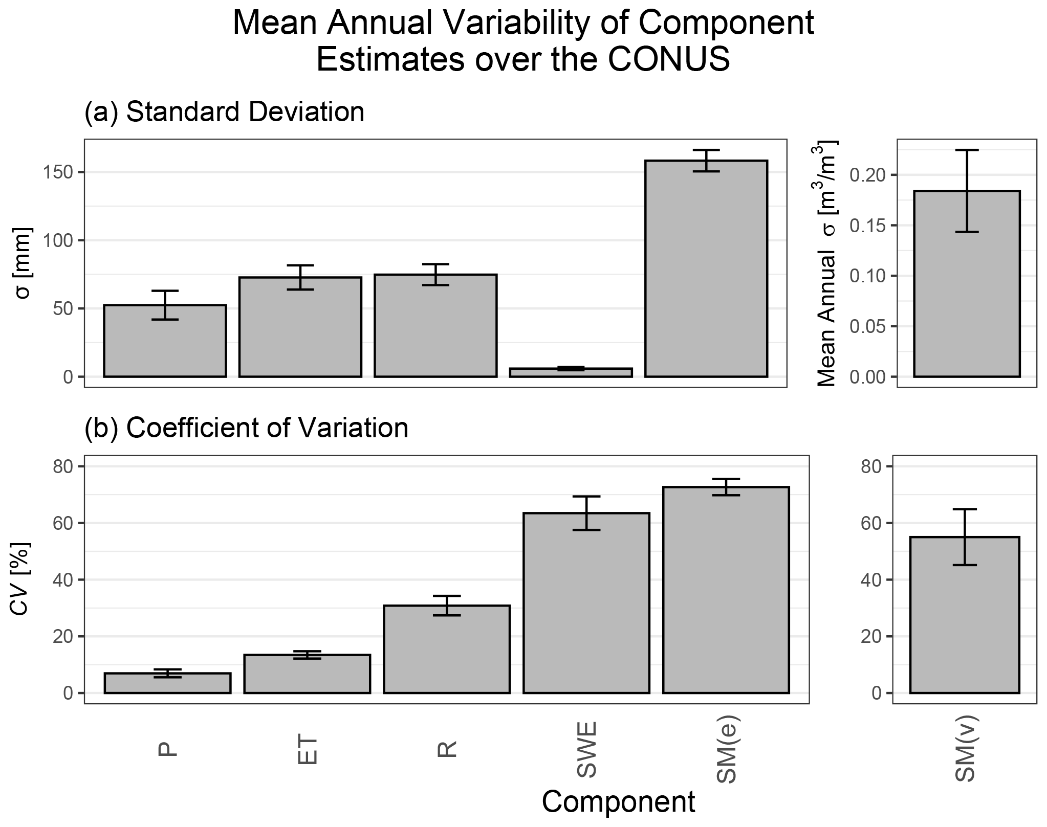
Figure 2 Mean annual (a) standard deviation (σ) and (b) coefficient of variation (CV) calculated between CONUS-extent modeled estimates of hydrologic components precipitation (P), evapotranspiration (ET), runoff (R), snow water equivalent (SWE), soil moisture in equivalent water depth (SM(e)), and soil moisture in volumetric water content (SM(v)). Whiskers on each bar represent the standard deviation of annual values.

Unfortunately, high-magnitude differences in SM (Fig. 3e, f) are likely strongly controlled by model-defined soil layer depth and, thus, limit the utility of disagreement statistics. For example, the TerraClimate and NLDAS2-Noah models apply spatially invariant root zone soil depth across the model domains (Abatzoglou et al., 2018; Xia et al., 2012a), whereas the NHM-PRMS assumes a variable depth according to vegetative and geophysical parameters (Regan et al., 2018). SM(e) estimates are directly controlled by soil depth, returning values of equivalent water depth. SM(v) differences are likely to be less influenced by soil depth due to inherent measurements of fractional volume rather than depth. However, soil water profiles can change significantly with depth, so attributing model differences strictly by root zone depth definition is more difficult.

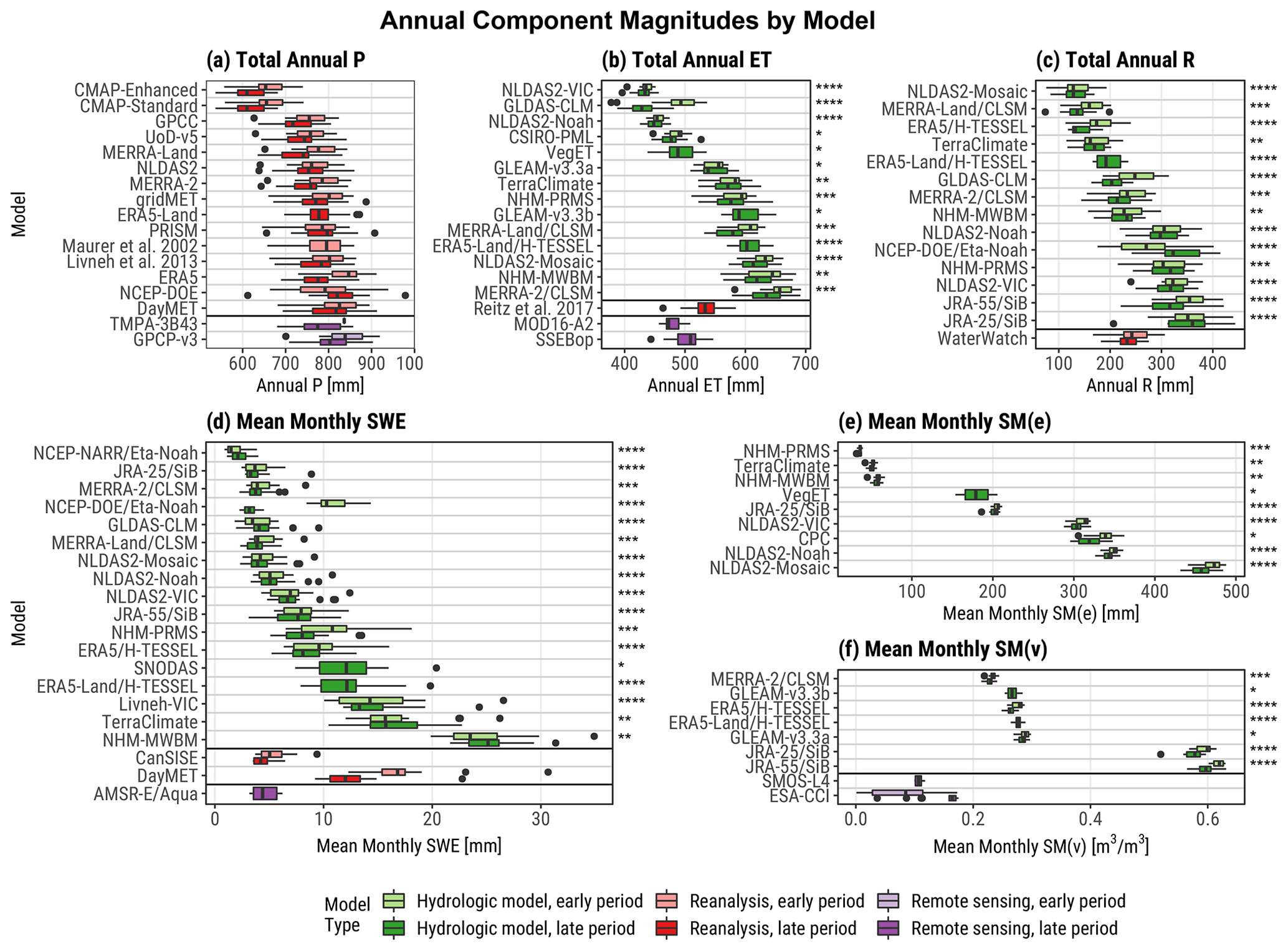
Figure 3 Box plots of annual water year magnitudes of all study model estimates averaged over the CONUS extent for hydrologic components (a) precipitation (P), (b) evapotranspiration (ET), (c) runoff (R), (d) snow water equivalent (SWE), (e)soil moisture in units of equivalent water depth (SM(e)), and (f) soil moisture in units of volumetric water content (SM(v)). Data set magnitudes are subdivided into two periods, i.e., 1985–1999 (top) and 2000–2014 (bottom), for each model. Flux component estimates (P, ET, and R) are summed from monthly values to calculate annual water year rates. Storage component estimates (SWE, SM(e), and SM(v)) are averaged from monthly values to calculate annual water year average storage values. Box lower limits, midlines, and upper limits represent the 25th, 50th (median), and 75th percentiles, respectively, of the associated data. Whiskers represent 1.5 times the interquartile range. Box color denotes data set categories of hydrologic model, reanalysis, or remote sensing derived. Asterisks are used to identify the following hydrologic models types: land surface models (${}^{****}$), catchment models (${}^{***}$), water balance models (${}^{**}$), and miscellaneous (^*).

Box plots of modeled estimates by water budget component (Fig. 3) demonstrate the annual ranges of magnitude generated by various products. Precipitation models (Fig. 3a) exhibit low overall variability, with median magnitudes falling within a distinct 100 mm per year (700–800 mm per year) range. The exceptions to this are the CMAP reanalysis data sets, which have a median 647 mm per year.

Variability among ET estimates (Fig. 3b) is higher, falling within a 200 mm per year (435–650 mm per year) range, though attributing differences to model type (e.g., LSMs vs. CMs) is difficult. Generally, CMs (MERRA-2/CLSM, MERRA-Land/CLSM, and NHM-PRMS) and conceptual WBMs (NHM-MWBM, GLEAM, and TerraClimate) produce greater annual rates of ET compared to LSMs (NLDAS2-VIC, GLDAS-CLM, and NLDAS2-Noah). Exceptions to this are the LSMs NLDAS2-MOSAIC and H-TESSEL that are more similar in annual ET flux to CMs and WBMs. The RS data sets agree more at the CONUS extent with lower-magnitude estimates.

Estimates of R show three distinct clusters of CONUS magnitudes (Fig. 3c) of 130–190, 220–242, and 310–345 mm per year. The NLDAS2-Noah and NLDAS2-VIC LSMs, which produced some of the lowest ET rates, fall within the higher-magnitude R clusters, as do the JRA-driven SiB models and NHM-PRMS model. The lowest magnitude estimates are the NLDAS2-Mosaic and ERA5-driven H-TESSEL LSMs, which are grouped with the CM MERRA-Land/CLSM and WBM TerraClimate. LSMs are more likely to estimate greater R than WBMs or CMs.

Box plots of annually averaged SWE monthly values (Fig. 3d) show that WBMs, notably the NHM-MWBM, generate much higher SWE than most other data sets. Alternatively, there are few discernible patterns between the remaining products, with LSMs and CMs interspersed throughout the gamut of median values. To generalize, the LSMs Noah, GLDAS-CLM, and NLDAS2-Mosaic produce lower-magnitude estimates of monthly SWE. A total of three different Noah estimates, driven with different meteorological forcings and run both independently (NLDAS2-Noah) or as part of a larger model (e.g., NCEP-NARR/Eta-Noah), all estimate lower SWE relative to other data sets. The two VIC LSMs show contrasting median monthly SWE magnitude over the CONUS, with the Livneh-VIC median exceeding the NLDAS2-VIC median by more than 200 %. The RS AMSR-E/Aqua product agrees more with lower-magnitude estimates at the CONUS extent.

Across all water budget components, most data sets demonstrate lower-magnitude values in the late period (WYs 2000–2014) compared to the early period (WYs 1985–1999). Within the P flux, almost all data sets agree on a decrease in the magnitude of hydrologic fluxes from the early to late periods. This is similarly reflected in the flux estimates of ET and R, and, to a less uniform extent, the storage components of SWE and SM. Several data sets, however, exhibit increased estimates from the early to late periods. For example, the NCEP–DOE reanalysis precipitation, and corresponding runoff derived by forcing the Noah LSM within the Eta atmospheric model, show increased median annual flux rates from the early to late periods.

3.1.2 Trends

Only 19 out of 87 component estimates exhibit statistically significant CONUS average domain trends, evaluated with Sen's slope, from 1982 to 2010 (Fig. 4). Within most components, one or more data sets produced a significant slope that is contradicted by one or more data sets. For example, the R estimates from LSMs GLDAS-CLM, JRA-55/SiB, and ERA5/H-TESSEL each show a significant negative trend in annual values across the CONUS over the 1982–2010 period. Conversely, the NCEP–DOE/Eta-Noah LSM shows a significant positive trend over the same period, and the remaining data sets, a mix of hydrologic and reanalysis models, show no significant trend. While the NCEP–DOE reanalysis precipitation trend matches that of the NCEP–DOE forced Eta-Noah, model estimates of SWE indicate a significant negative trend.

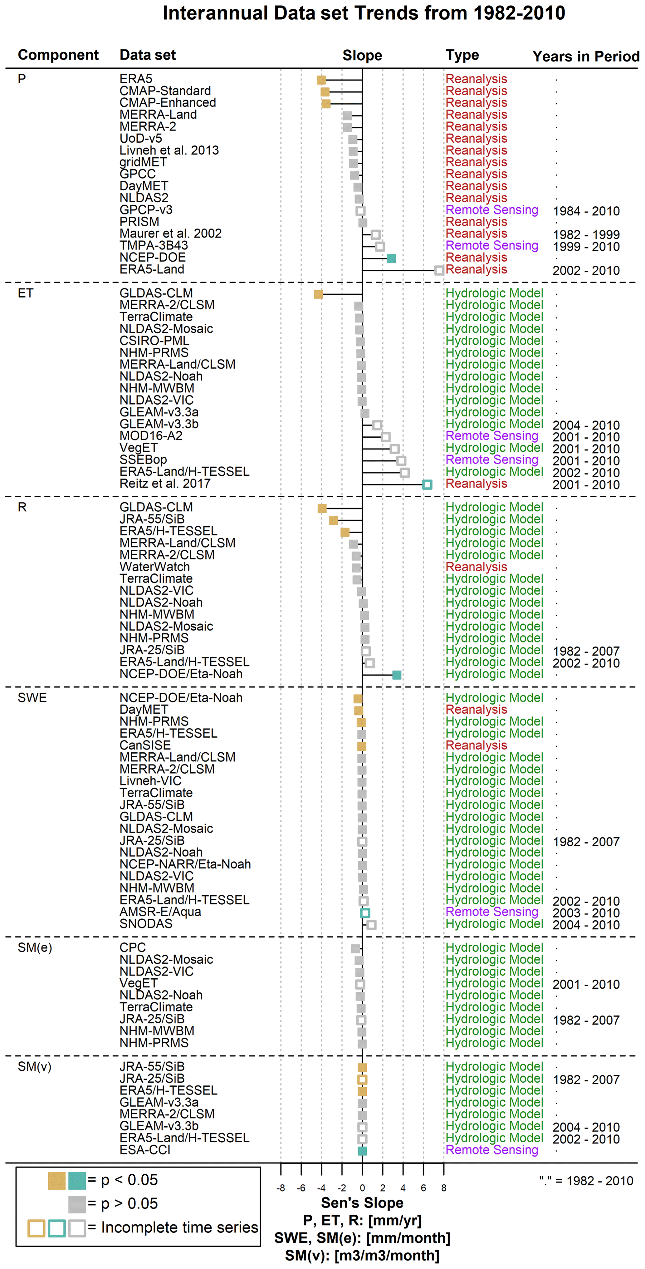
Figure 4 Forest plot of interannual (water year) component estimate Sen's slope from 1982 to 2010 for components of precipitation (P), evapotranspiration (ET), snow water equivalent (SWE), soil moisture in units of equivalent water depth (SM(e)), and soil moisture in units of volumetric water content (SM(v)). Insignificant trends (p>0.05) are gray. Significant trends are colored based on direction, where negative trends are gold and positive trends are green. Data sets without complete data during the study period are represented with hollow points, and the temporal extent is noted under “Years in Period” column.

3.2 Ecoregions

3.2.1 Magnitude variability

Uncertainty in modeled hydrologic component estimates in each ecoregion is presented in terms of CV (Fig. 5) and σ (Appendix A). Ecoregions are organized from west to east within each figure. Results and discussion of uncertainty are focused primarily on CV due to the disparity in annual water flux between regions. By component, P and ET estimates demonstrate lower uncertainty compared to other hydrologic components (Fig. 5a, b). P estimates typically range in median uncertainty from 5 % to 14 % in the eastern CONUS and 11 % to 21 % in the western CONUS. P uncertainty is highest in mountainous regions with more variable topography (e.g., Northwestern Forested Mountains and Temperate Sierras) and lowest in more humid, topographically homogeneous regions (e.g., Eastern Temperate Forests).

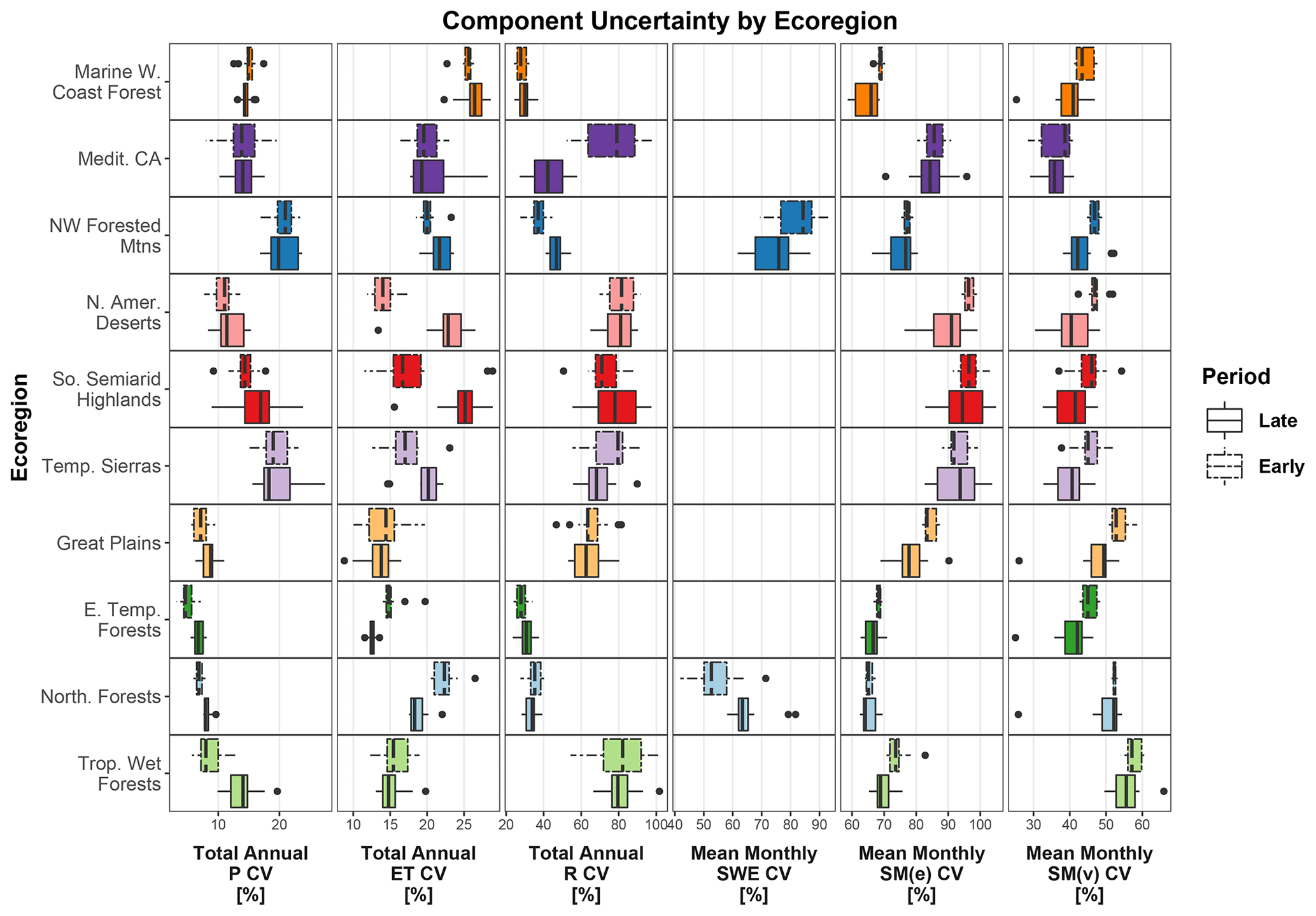
Figure 5 Box plots of uncertainty, measured as annual coefficient of variation (CV), between component estimates at 10 ecoregions. CV distributions are subdivided into late and early periods, i.e., 1985–1999 and 2000–2014. Box lower limits, midlines, and upper limits represent the 25th, 50th (median), and 75th percentiles, respectively, of the associated data. Whiskers represent 1.5 times the interquartile range. Box colors denote the ecoregion and correspond to the map colors in Fig. 1. Components displayed are precipitation (P), evapotranspiration (ET), runoff (R), snow water equivalent (SWE), soil moisture in units of equivalent water depth (SM(e)), and soil moisture in units of volumetric water content (SM(v)). Results for SWE uncertainty are omitted for ecoregions with limited annual snowpack.

The median uncertainties of ET estimates typically range from 13 % to 22 % in the eastern CONUS ecoregions and 14 % to 26 % in the western CONUS. Uncertainty is greatest along the Pacific coast and northerly ecoregions and arid and semiarid ecoregions that are heavily influenced by anthropogenic water use. Of the four largest ecoregions (Table 2), Northwestern Forested Mountains and North American Deserts demonstrate mean uncertainties of 21 % and 19 %, respectively, and the Great Plains and Eastern Temperate Forests demonstrate mean uncertainties of 14 % each.

Estimates of R (Fig. 5c) generally exceed 29 % variability throughout the study ecoregions, with median values reaching or exceeding 72 % in arid, snow-sparse western ecoregions of North American Deserts, Southern Semiarid Highlands, and Temperate Sierras, as well as in Tropical Wet Forests influence by tropical storm systems. In the large Northwestern Forested Mountains and Great Plains ecoregions, median data set variability is 28 % to 55 % and 47 % to 81 %, respectively.

SWE estimate uncertainty is highlighted for the snow-dominated Northwestern Forested Mountains and Northern Forests ecoregions (Fig. 5d), where annual peak SWE values exceed estimated snowpack in the remaining ecoregions by up to 700 % (Fig. B2). Of primary interest is the Northwestern Forested Mountains ecoregion that contains the snowmelt-dominated regimes of the Rocky, Sierra Nevada, and Cascade mountain ranges that are strong contributors to water supply for population centers such as Denver, Los Angeles, San Francisco, Portland, and Seattle. In this ecoregion, modeled estimates of monthly mean SWE storage vary by 76 % to 84 %, equating to median equivalent water depth standard deviations as high as 48 mm per month.

SM(e) estimate uncertainty (Fig. 5e) is greatest, 66 %–96 %, in arid western ecoregions, though other regions fall within a 64 %–83 % uncertainty range. SM(v) shows lower overall uncertainty (Fig. 5f), with less dramatic differences between regions, ranging from 36 % to 57 %, with the greatest uncertainty (44 %–57 %) in central and eastern CONUS ecoregions. As mentioned previously, uncertainty in SM estimates, most importantly SM(e), is strongly influenced by model-defined root zone soil thickness. Spatial differences in SM(e) uncertainty measured as CV, therefore, are pronounced in regions with lower water content because CV, a measure of relative variability, is more strongly affected by magnitude differences. Because the range of values is constrained from 0 to 1 in m³ per cubic meter, uncertainty in SM(v) is less influenced by spatial variability in soil water magnitudes and is therefore a better measure for understanding regional soil water estimate disagreement. Following this logic, SM(v) uncertainty is greater in Tropical Wet Forests, Northern Forests, and Great Plains ecoregions, with an average CV of 53 % compared to an average of 42 % for the remaining ecoregions.

3.2.2 SWE accumulation and ablation

Timing of SWE estimates is presented in terms of relative timing (Figs. B3 and B4). Figures are divided by Northern Forests and Northwestern Forested Mountains ecoregions, trends of accumulation and ablation, and early and late periods. Negative (positive) values in purple (green), identify models for which accumulation or ablation begins more than 1 month earlier (later) than the mean of other data sets. Distributions of relative timing by year are presented in Fig. B3 and summarized as the percentage of years that are positive or negative in Fig. B4. In both ecoregions, uncertainty among data sets is greater in ablation timing than accumulation timing, and overall uncertainty is greater in the Northwestern Forested Mountains ecoregion than in the Northern Forests.

Relative timing between models can be similar between ecoregions (Figs. B3a and B4), especially regarding accumulation. For instance, the AMSR-E/Aqua RS and NHM-MWBM CM consistently show later accumulation start dates than other data sets in both ecoregions, while the ERA5-Land/H-TESSEL, JRA-55/SiB, and SNODAS models estimate earlier accumulation dates. Conversely, the JRA-25/SiB and TerraClimate models show different trends in accumulation timing between regions with earlier SWE accumulation in Northern Forests but later accumulation in Northwestern Forested Mountains.

Regarding ablation, outliers are much more common when comparing models (Figs. B3b and B4). For example, the Daymet model consistently estimates a much later start of spring ablation while the Eta-Noah models driven with NCEP–DOE and NCEP-NARR reanalyses typically estimate much earlier ablation times, often 1–2 months after the mean antecedent month (Fig. B3). Uncertainty in ablation timing is typically much higher in the Northwestern Forested Mountains ecoregion than in the Northern Forests. The Daymet, ERA5-Land/H-TESSEL, Livneh-VIC, NLDAS2-VIC, and SNODAS models commonly estimate a later start to ablation than the remaining models.

Models that predict earlier (later) accumulation timing and later (earlier) ablation timing represent longer (shorter) periods of growing or available snowpack (Fig. B4). The ERA5-Land/H-TESSEL, Livneh-VIC, and SNODAS models estimate longer snowpack periods than other models in both ecoregions. The AMSR-E/Aqua, JRA-55/SiB, NHM-PRMS, and TerraClimate models estimate longer snowpack periods in only one ecoregion. The NCEP-NARR/Eta-Noah, NLDAS2-Mosaic, and NLDAS2-Noah models estimate shorter snowpack periods in the Northern Forests ecoregion while the GLDAS-CLM and JRA-25/SiB models estimate shorter snowpack periods in the Northwestern Forested Mountains ecoregion.

Attributing the relative timing of SWE to model type is difficult at the monthly scale. LSMs estimate both earlier and later accumulation and ablation antecedences, and the two WBMs in this study show opposing timing trends. Similarly, grouping by organization does not yield significant similarities. For example, the timing of NLDAS2-driven LSMs from the National Aeronautics and Space Administration (NASA) is dissimilar from that of the MERRA-2-driven and MERRA-Land-driven CLSM, which are also from NASA. Forcing data also do not yield useful information for identifying controlling variables. Only the NLDAS2-driven models from NASA tend to all show later (earlier) accumulation (ablation) timing. Even the Eta-Noah LSMs, driven by the NCEP–DOE reanalysis and the corresponding higher-resolution version for North America NCEP-NARR show different relative timing values in both ecoregions.

3.2.3 Trend

Interannual trend analyses performed with the Mann–Kendall trend test (τ) over water years 1982–2010 show varying degrees of agreement and disagreement between ecoregions. Figures showing explicit distributions of trends with model names are supplied in the appendix (Fig. B5). Model disagreement in trend direction is quantified using the unalikeability coefficient (u; Fig. 6), with 0 and 1 being complete agreement and disagreement, respectively.

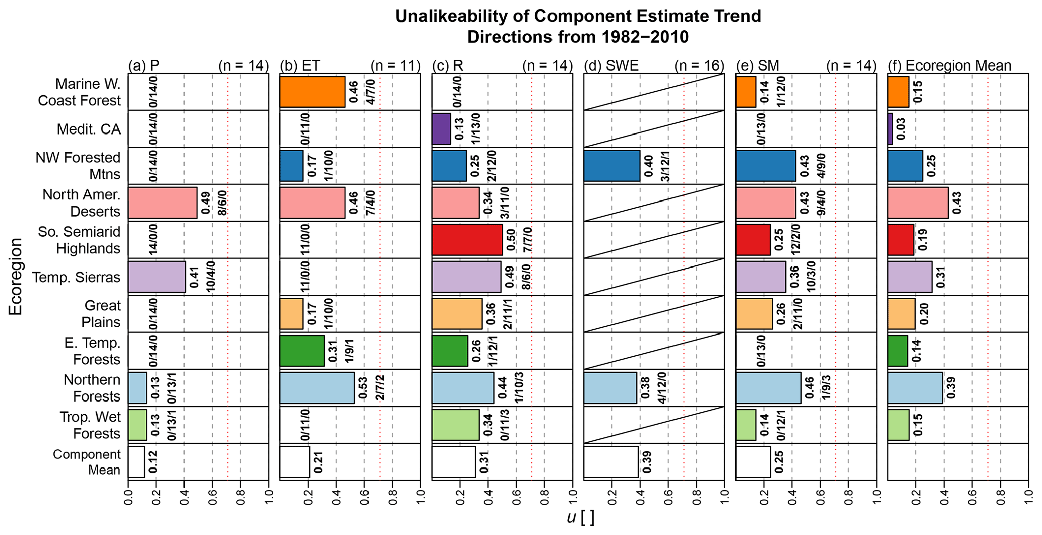
Figure 6 Bar plots summarizing the disagreement in Mann–Kendall trend (τ) direction using the unalikeability coefficient (u) after categorizing τ as significant negative trend, significant positive trend, or no significant trend for 10 ecoregions from 1982 to 2010. Trends were assumed to be significant if p<0.05. u can range from complete agreement (u=0) to complete disagreement (u=1) when sample size (n) is less than the number of categorical values (c). Because here n>c, maximum possible u is approximately 0.71 (dotted red line). Text to the right of each bar shows, in order, the u value and the number of data sets showing the negative, insignificant, or positive trend. Bars are color matched to ecoregion colors from Fig. 1 and are ordered from west (top) to east (bottom). Results are provided for water balance components of precipitation (P), evapotranspiration (ET), runoff (R), snow water equivalent (SWE), and soil moisture (SM) in units of either equivalent water depth or volumetric water content.

Precipitation estimates demonstrate the lowest u, showing no (u=0) to low (u=0.13) disagreement in eight ecoregions where data sets show no significant τ (Fig. B5a). Disagreement is higher in North American Deserts and Temperate Sierras ecoregions (u= 0.41–0.49) where most data sets show a negative τ, and all data sets show a negative τ in the Southern Semiarid Highlands. Coefficient u is higher among ET data sets than P data sets, averaging 0.21 across ecoregions, notably in the North American Deserts and Marine West Coast Forest ecoregions (u=0.46 and 0.53), where negative and insignificant τ values are present (Fig. B5b). All data sets identify negative ET τ in the Southern Semiarid Highlands and Temperate Sierras. Data sets show positive, negative, and insignificant τ in the Eastern Temperate Forests (u=0.31) and Northern Forests (u=0.53). Runoff data sets show the most consistent spatial distribution of u>0 across the study ecoregions. Disagreement in the western ecoregions is caused by conflicting negative and insignificant Rτ (Fig. B5c), with the greatest u in the Southern Semiarid Highlands (u=0.50) and Temperate Sierras (u=0.49). Eastern ecoregion τ is generally caused by conflicting positive, negative, and insignificant τ values (u= 0.26–44). Ecoregions with good agreement (u= 0–0.35) are generally due to most data sets showing no significant trend.

SWE data sets, limited in this study to the Northwestern Forested Mountains and Northern Forests, show disagreement, i.e., u=0.42 and 0.40, respectively, mostly caused by conflicting negative and insignificant τ, though most data sets show no significant trend (Fig. B5d). Trend agreement is better among SM data sets (mean u= 0.25), though higher u is noted in the Northwestern Forested Mountains, North American Deserts, and Northern Forests and is caused by conflicting negative and insignificant τ values. Ecoregions with low u typically show no significant τ values in SM data sets, except for the Southern Semiarid Highlands where most data sets show a significant negative τ.

Generally, τ disagreement is highest in the North American Deserts and Northern Forests ecoregions and lowest in the Mediterranean California, Eastern Temperate Forests, Marine West Coast Forest, and Tropical Wet Forests ecoregions. Trend disagreement is almost always caused by conflicting negative and insignificant trends, indicating that disagreement is due to the occurrence, and not the direction, of the trend. That is to say, higher u values are caused by disagreement over whether there is or is not a significant trend present in the data, as opposed to higher u values being caused by disagreement between significant negative and significant positive trends.

3.2.4 Correlation with remote sensing

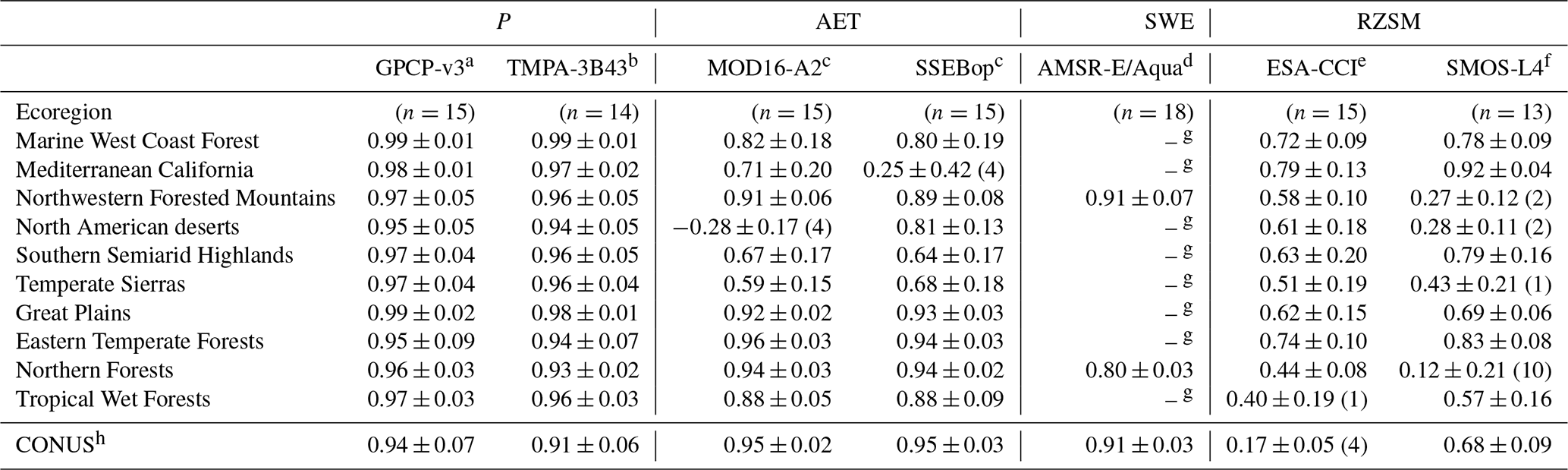
Spearman's rho (ρ) correlation was calculated for all hydrologic models and reanalysis data sets against remote sensing products with 48 or more months of intersecting temporal extents (Fig. 7; Table 3). Precipitation data sets (Fig. 7a, b), correlated against the GPCP-v3 and TMPA-3B43 products, show high correlation compared against 13 data sets (ρ= 0.93–0.99) with no statistically insignificant values. Variability in P estimate correlations are low (± 0.01–0.09). ET data sets correlated against the MOD16-A2 and SSEBop products (Fig. 7c, d) show poorer correlation in western ecoregions, with mean ρ ranging from 0.59 to 0.91. Extreme cases are found when correlating against MOD16-A2 in North American Deserts ($\mathit{\rho }=-\mathrm{0.28}$) and SSEBop in Mediterranean California (ρ=0.25), where four data sets show insignificant ρ. The exception in the western CONUS is in Northwestern Forested Mountains, where models correlate against both RS data sets well (MOD16-A2 ρ= 0.91 and SSEBop ρ= 0.89). Correlation against both products is high in eastern ecoregions, ranging from ρ= 0.88 to 0.96, with standard deviation decreasing as ρ increases.

Table 3 Spearman's rho (ρ) correlation of monthly hydrologic model and reanalysis data set estimates against remote sensing products quantifying hydrologic components precipitation (P), evapotranspiration (ET), snow water equivalent (SWE), and soil moisture (SM). Correlation was calculated at 10 ecoregions and at the CONUS extent. The number of modeled data sets correlated against remote sensing products is shown as (n=X) for each column. Mean and standard deviation (σ) of ρ are provided for each ecoregion and remote sensing products as ρ±σ. Counts of statistically insignificant correlations (Y) are denoted when n>0 as (Y). SM combines data sets produced in units of equivalent water depth (SM(e) in text) and volumetric soil moisture water content (SM(v) in text). Correlation of SWE products is included only for regions of high annual mean SWE storage. Hydrologic model and reanalysis data sets (Table 1) used in each column are listed in the footnotes.

^a CMAP enhanced and standard, Daymet, ERA5, ERA5-Land, GPCC, gridMET, Livneh et al. (2013), Maurer et al. (2002), MERRA-2, MERRA-Land, NCEP–DOE, NLDAS2, PRISM, and UoD-v5.
^b CMAP enhanced and standard, Daymet, ERA5, ERA5-Land, GPCC, gridMET, Livneh et al. (2013), MERRA-2, MERRA-Land, NCEP–DOE, NLDAS2, PRISM, and UoD-v5.
^c CSIRO-PML, ERA5-Land/H-TESSEL, GLDAS-CLM, GLEAM-v3.3a and v3.3b, MERRA-2 and MERRA-Land/CLSM, NHM-MWBM and NHM-PRMS, NLDAS2-Mosaic, NLDAS2-Noah, NLDAS2-VIC, Reitz et al. (2017), TerraClimate, and VegET.
^d CanSISE, Daymet, ERA5-Land/H-TESSEL, GLDAS-CLM, JRA-25 and JRA-55/SiB, Livneh-VIC, MERRA-2 and MERRA-Land/CLSM, NCEP–DOE and NCEP-NARR/Eta-Noah, NHM-MWBM and NHM-PRMS, NLDAS2-Mosaic, NLDAS2-Noah, and NLDAS2-VIC, SNODAS, and TerraClimate.
^e CPC, ERA5-Land and ERA5/H-TESSEL, GLEAM-v3.3a and v3.3b, JRA-25 and JRA-55/SiB, MERRA-2/CLSM, NHM-MWBM and NHM-PRMS, NLDAS2-Mosaic, NLDAS2-Noah and NLDAS2-VIC, TerraClimate, and VegET.
^f CPC, ERA5-Land and ERA5/H-TESSEL, GLEAM-v3.3a and v3.3b, JRA-55/SiB, MERRA-2/CLSM, NHM-PRMS, NLDAS2-Mosaic, NLDAS2-Noah, and NLDAS2-VIC, TerraClimate, and VegET.
^g Regions omitted.
^h Calculated from data sets spatially aggregated by weighted area mean at the CONUS extent (Fig. 1) and not as a mean of individual ecoregion ρ estimates above.

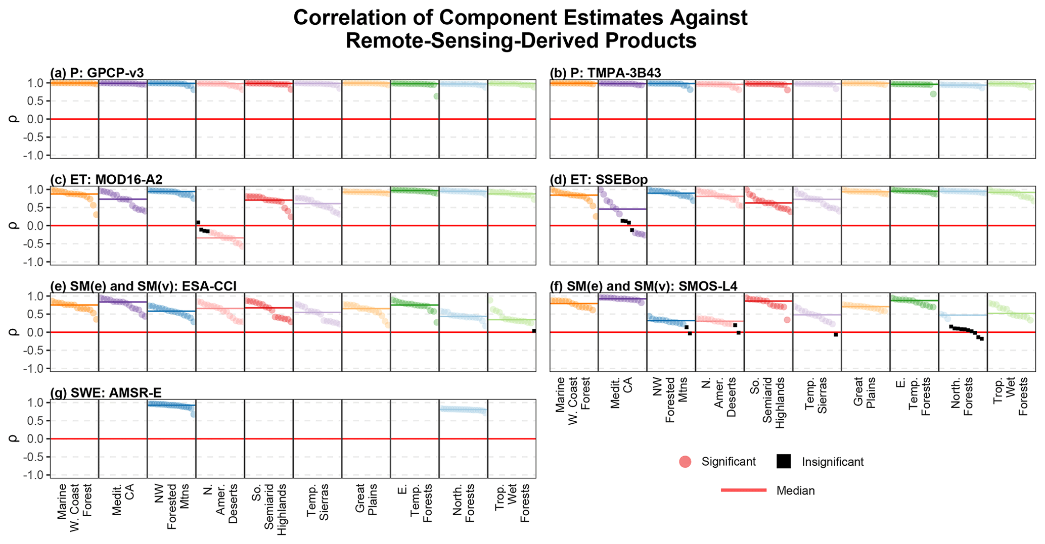
Figure 7 Spearman's rho (ρ) correlation values of hydrologic model and reanalysis data set component estimates against remote-sensing-derived products for components of precipitation (P), evapotranspiration (ET), soil moisture in units of both equivalent water depth (SM(e)) and volumetric water content (SM(v)), and snow water equivalent (SWE). The title of each sub-plot (e.g., Fig. 7a) provides the hydrologic component (e.g., P) and the remote sensing product against which the data set was correlated (e.g., GPCP-v3). Statistically significant ρ values (p<0.05) are shown as colored circles. Insignificant ρ values (p>0.05) are shown as black squares. Horizontal bars within each ecoregion denote mean ρ. Point and bar colors correspond to ecoregions, as shown in Fig. 1. Each point or square corresponds to a single modeled data set, with points sorted by descending ρ value. More detailed information can be found in Fig. B6.

SWE data sets correlated against the AMSR-E/Aqua product are highlighted for the Northwestern Forested Mountains and Northern Forests ecoregions (Fig. 7e). Modeled estimates correlate better in the Northwestern Forested Mountains (ρ=0.91) than Northern Forests (ρ=0.80). SM data sets show worse and more variable ρ against remote sensing products ESA-CCI and SMOS-L4 (Fig. 7f, g) than other components. At the CONUS scale, estimates correlate very poorly against the ESA-CCI product (ρ=0.17) and only moderately well against SMOS-L4 (ρ=0.68). Generally, correlation is best in the Mediterranean California and Eastern Temperate Forests ecoregions (ρ= 0.74–0.92). Correlation is worst in Northwestern Forested Mountains, North American Deserts, and Northern Forests (ESA-CCI ρ= 0.44–0.61; SMOS-L4 ρ= 0.12–0.28). Explicit distributions of correlation for each data set by ecoregion are provided in Fig. B6.

3.2.5 Case study – impact of model selection on water budget imbalances

A case study calculating 2925 10 year water budgets (WY 2001–2010) using 15 P, 15 ET, and 13 R estimates for each of the 10 ecoregions was performed to demonstrate quantitatively how model selection can affect research results. Each water budget was solved for a relative imbalance (Rε) with Eq. (7), which estimated the model error as a fraction of total water flux in P.

Histograms of the results, overlain with box plots (Fig. 8), demonstrate the range and distribution of potential water budget Rε values. In most ecoregions, Rε values exhibit an approximately normal distribution. The following four ecoregions dominating the area of the CONUS (Fig. 8a–d), constituting 90 % of the CONUS area (Table 2), are the focus of these results: the western ecoregions of the Northwestern Forested Mountains and North American deserts and the eastern ecoregions of the Great Plains and Eastern Temperate Forests (11 %, 19 %, 29 %, and 31 % of the CONUS area, respectively).

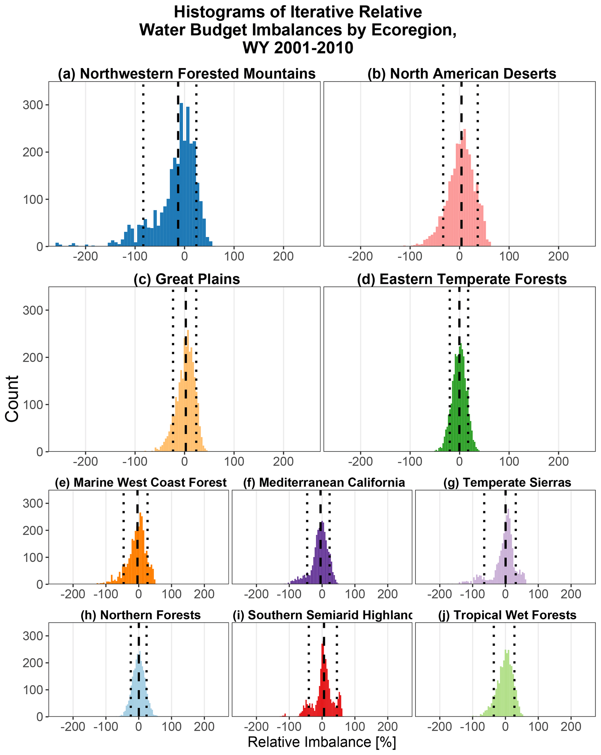
Figure 8 Histograms of 10 ecoregion water budget relative imbalances calculated from combinations of all annual precipitation (15), evapotranspiration (15), and runoff (13) data sets with complete data from water years 2001–2010 (Table 1). Each region yielded 2925 water budgets. Relative imbalances are calculated as a percentage of annual P. The 10th and 90th percentiles of each ecoregion distribution are provided as vertical dotted lines. Dashed vertical lines represent the relative imbalances of 10 year (2001–2010) water budgets from the ensemble mean of all modeled products.

Of these larger domains, water budget Rε values in the eastern ecoregions show much lower variability (Table 4), with the Great Plains and Eastern Temperate Forests yielding σ values of 18.2 percentage points and 14.3 percentage points, respectively, and medians of 3.9 % and −0.4 %, respectively. Similarly, the 10th and 90th percentiles (P10 and P90) are −23.2 % and 23.6 % for the Great Plains and −19.9 % and 17.2 % for the Eastern Temperate Forests. In contrast, the major western ecoregions exhibit much higher variability, with Northwestern Forested Mountains and North American Desert σ values of 45.6 % and 27.0 %, respectively, and medians of −6.7 % and 4.7 %, respectively. P10 and P90 are higher than eastern regions as well, yielding −83.3 % and 23.8 % for the Northwestern Forested Mountains and −33.2 % and 36.6 % for the North American Deserts. Smaller ecoregions (Fig. 8e–j) yield similar spatial trends in variability, with the eastern Northern Forests ecoregion showing lower σ and P10 and P90 than the western Marine West Coast Forest and Mediterranean California ecoregions.

The Northwestern Forested Mountains region, accounting for 11 % of the CONUS area, is unique among ecoregions in this study. It exhibits the greatest magnitude of variability in iterative water budget Rε, P10–P90 Rε ranges, skewness (−1.6), and kurtosis (3.7). Furthermore, the difference between the ensemble water budget Rε and median iterative water budget Rε is greater than any other ecoregion (−6.3 points).

4 Discussion

Results of model comparisons demonstrate the effect that model disagreement can have on both regional- and continental-scale research. Comparisons of P estimates agree with previous findings (Derin and Yilmaz, 2014; Guirguis and Avissar, 2008; Sun et al., 2018), noting increased uncertainty between products in regions of complex topography. ET comparisons showed that LSMs are more likely to produce lower annual ET than CMs and WBMs, similar to results found by Mueller et al. (2011), and that model disagreement is higher in Pacific regions, similar to the comparison and validation of MOD16-A2, NLDAS2-Noah, and ALEXI by Carter et al. (2018). However, this paper finds some differences from the work of Carter et al. (2018) and notes a higher uncertainty of ET estimates in arid, semiarid, and mountainous regions, as well as lower uncertainty in eastern regions. Haddeland et al. (2011) found that LSMs underestimate R partitioning relative to global hydrologic models (not used in this paper). Here, we find that LSMs are more likely to estimate greater R than either WBMs or CMs. Xia et al. (2012a, b) noted greater model disagreement in R estimates between several LSMs in the northeastern and western mountainous regions of the CONUS. This paper, using CV as a measure of relative uncertainty, alternatively shows that modeled runoff uncertainty is higher in the arid and semiarid regions of the western CONUS where annual R rates are lower.

Table 4 Summary statistics of ecoregion water budget calculations summed for complete water years 2001–2010. Median (P₅₀) and standard deviation (σ) summarize the iterative water budgets' (n=2925) relative imbalances (Rε) in units of percent. The 10th, 25th, 75th, and 90th percentiles (P_i) quantify the distribution ranges, along with skew (γ) and kurtosis (K). The ensemble column μ provides water budget Rε produced from the ensemble mean of all data sets available for water years 2001–2010.

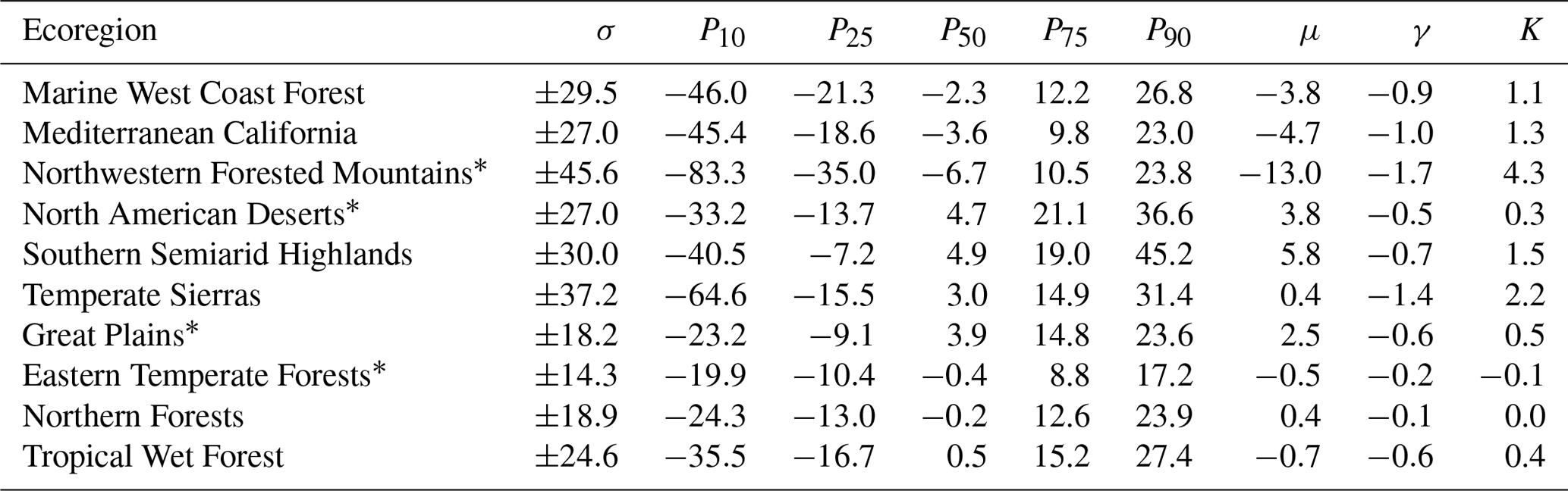
^* Primary focus ecoregions.

Previous analyses of modeled SWE estimates focused largely on the validation of winter snowpack magnitudes against the SNODAS model or on the timing of accumulation and ablation periods. Broxton et al. (2016) found that LSMs estimated earlier ablation timing than observational measurements, in contrast with the results of Essery et al. (2009) and Rutter et al. (2009), who noted later timing in LSMs. Our results indicate the alternative argument that neither snow accumulation nor ablation timing can be accurately attributed solely to model design and note differences in relative timing of as much as 2 months between LSMs. In contrast to the arguments by Murdryk et al. (2015) and Broxton et al. (2016), who concluded that uncertainty in estimates may be controlled by differences in model structure, the results here show that attributing model differences to structure is likely impossible without controlling for forcing data, model parameters, and calibration methods. Properly identifying controls on model differences requires robust MIPs wherein hydrologic models are operated within the confines of strict input data and calibration schemes, such as those performed by Haddeland et al. (2011), Kollet et al. (2017), or Rosenzweig et al. (2013).

Perhaps the most important variable controlling uncertainties in SM(e) is the discrepancies in model-defined root zone depth. Typically, the largest surface storage component in the hydrologic cycle, i.e., differences in SM(e) estimates, will more greatly affect water availability calculations than any other component. Koster et al. (2009) argued that modeled soil moisture, related in units of equivalent water depth (i.e., SM(e)), should not be considered direct measures of actual soil water content but should instead be used as relative values to identify seasonal to annual trends and responses to changing climatology. However, LSM estimates of soil moisture depth are commonly applied in research applications as direct measures of soil water content. For example, groundwater storage trends are calculated from Gravity Recovery and Climate Experiment (GRACE) solutions of terrestrial water storage anomalies (Rodell et al., 2007; Scanlon et al., 2012; Thomas and Famiglietti, 2019; Voss et al., 2013). Groundwater storage is calculated as the remainder after removing surface storage components, such as modeled surface water storage, SWE, and SM(e) storage values, from GRACE terrestrial water storage. Because estimates of SM(e) can vary by 64 % to 96 %, groundwater storage values derived from GRACE solutions will be significantly affected. Groundwater storage values are most commonly extracted using the NLDAS2- or GLDAS-driven LSMs of Mosaic, Noah, VIC, or CLM that agree more in monthly SM(e) magnitude than with other estimates from WBMs or CMs. However, even those products show differences in SM(e) estimates of up to 250 mm per year. Therefore, quantifying differences in SM(e) is useful in understanding the uncertainty propagation in research results.

In terms of evaluating surface water availability, snowmelt from the Northwestern Forested Mountains ecoregion is a primary supply of water for many western population centers. However, disagreement between models of annual snowpack in this study, measured as SWE, averages 97 %, and relative variability and timing on accumulation or ablation can vary by up to 2 months. These levels of disagreement strongly affect the accuracy of predictive and retrospective snow water analyses of both present snowpack and long-term trends.

LSMs, typically targeted to estimate the vertical ET flux, generally overestimate R compared to CMs. Conversely, CMs, targeted to estimate the horizontal R flux, often overestimate ET compared to LSMs. This is likely an example of equifinality (Beven, 2006), wherein target variable accuracy may be reached without accurately representing the complete hydrologic system. In comparing model output by organization, estimates of P, ET, and SWE produced by NASA are often lower in magnitude than those produced by the USGS and European Centre for Medium-Range Weather Forecasts (ECMWF), indicating organizational differences in model operation methods, such as forcing data selection or calibration methodology.

Results of the water budget case studies demonstrate that water budget Rε values are more variable in the western CONUS, with σ of ± 27.0 % to 45.6 % by ecoregion, although even eastern CONUS Rε values range in variability from ± 14.3 % to 18.9 % by ecoregion. In all regions, various combinations of products can result in both positive and negative imbalances (ε), yielding alarmingly different research implications. Positive ε (P>ET+R) means that more water is entering a system than leaving. Assuming a limited influence of model uncertainty, this would imply that excluded natural or anthropogenic fluxes are removing water from the $P=\mathrm{ET}+R$ system. This could be interpreted as the presence of long-term natural contributions to storage components, such as soil moisture or groundwater, or as the presence of anthropogenic extractions. The same region, depending on the models selected, could yield negative ε (P<ET+R), implying the presence of additive fluxes such as releases from surface storage or increased irrigation from imported water.

Results in this paper supplement the work of Haddeland et al. (2011), who argued that climate change effect modeling on large-scale hydrologic processes should utilize a range of model estimates rather than rely on a single model realization. Indeed, we show that model variability in storage components often exceeds the magnitude of the measurements themselves, calling into question the functional application of terrestrial storage estimates. Our work shows that ensembles of model estimates are not only useful but are in fact a necessity for better understanding and quantifying current knowledge of terrestrial hydrology. Improved ensembling methods, as was done by Zaherpour et al. (2019), will likely be invaluable resources in the fields of terrestrial hydrology, climatology, and meteorology modeling. Work by Newman et al. (2015) and Addor et al. (2017) organized numerous modeled data sets across hundreds of watersheds in the USA through the Catchment Attributes and MEteorology for Large-sample Studies (CAMELs) data set, compiling meteorological, geophysical, and hydrologic response variables. Data hosted within the CAMELs data set, and the data sets prepared for this study (Saxe et al., 2020), reduce the workload for users for a better understanding of the inherent uncertainty in modeled products. This comprehensive and systematic comparison helps elucidate where we, as a scientific community, could better target research efforts to reconcile large-extent estimates of the hydrologic cycle. Most importantly, differences in modeled SM(e), both in terms of magnitude depth and correlation against RS products, would need to be addressed at the continental scale to better understand the largest surface store. Furthermore, estimates in SWE, ET, and R need to be reconciled in much of the western CONUS to provide a more accurate retrospective and operational overview of the hydrologic cycle. Finally, differences in hydrologic estimates warrant incorporation into future analysis that use these products to provide the scientific community with a more robust understanding of results confidence and areas of uncertainty. All data sets explored in this paper are easily obtained from publicly available sources, and modern data-processing workflows are applied to multiple data sets without difficulty.

5 Conclusions

Model selection can significantly alter results and findings when used as a substitute for observational data. Publicly available modeled estimates are commonly used within the scientific community, though the literature that effectively evaluates differences in magnitude and trend in the context of application is rare. MIPs abound within the scientific literature, often focusing on the causes of model disagreement (e.g., forcing data, model structure, and calibration) and validating against in situ observational data despite limited availability. In contrast, this study investigated how publicly available modeled estimates of hydrologic flux and storage components can affect scientific analyses by quantifying the disagreement between numerous hydrologic models, reanalysis data sets, and remote sensing products.

Results show that flux and storage magnitudes disagree most greatly in the western CONUS, with uncertainty (measured as a coefficient of variation) ranging from 11 % to 21 % for precipitation (P), 14 % to 26 % for evapotranspiration (ET), 28 % to 82 % for runoff (R), 76 % to 84 % for snow water equivalent (SWE), and 36 % to 96 % for soil moisture (SM). In the eastern CONUS, uncertainty is somewhat lower, ranging from 5 % to 14 % for P, 13 % to 22 % for ET, 28 % to 82 % for R, 53 % to 63 % for SWE, and 42 % to 83 % for SM. Interannual trends in estimates from 1982 to 2010 show more comprehensive agreement for P and ET fluxes, but common disagreement for R, SWE, and SM. Disagreement in trends (i.e., positive versus negative versus insignificant) between models is typically a result of conflicting negative and insignificant trends rather than between negative and positive trends, indicating that the disagreement is due to the occurrence and not the direction of trend. Correlating fluxes and stores against remote-sensing-derived products show poor overall correlation in the western CONUS for ET and SM. P correlates well in all regions, and SWE correlates well in the primary regions of Northwestern Forested Mountains and Northern Forests.

A water budget analysis, performed by iterating through all combinations of publicly available modeled products highlighted in this research, shows that in large eastern ecoregions the model selection can result in relative imbalances ranging from −50 % to 50 %. In larger western ecoregions, relative imbalances can range from −150 % to 60 %.

Publicly available modeled estimates of the hydrologic system accelerate the development of scientific research by reducing the necessary workload, processing time, and technical expertise for researchers. In addition, estimates fill knowledge gaps in fluxes and stores where observational data are incomplete. Metrics of disagreement in component estimates presented here help to describe the uncertainty of the scientific community's current state of knowledge. The uncertainty inherent in modern data sets can affect the results of studies as diverse as satellite-derived groundwater estimates and predictive snowmelt analyses. Our results highlight problem areas within CONUS-extent hydrologic estimation efforts that warrant better understanding and addressing in future endeavors. Most importantly, our results show that the most important issues to reconcile are disagreement, in terms of both magnitude and long-term trend, and of (a) SM storage across the CONUS, (b) SWE storage in western mountains, and (c) hydrologic fluxes in western arid and semiarid regions. Additionally, our results support the findings of previous studies and agree that future work applying modeled data would prove to be more accurate, more informative, and more robust by incorporating model ensembles to provide confidence intervals, better quantify result uncertainty, and improve overall accuracy.

Appendix A

Acronym	Product description
Hydrologic models
CPC	Climate Prediction Center
	Root zone soil moisture (equivalent water depth) estimated through a one-layer water balance model forced by CPC reanalysis precipitation and temperature. Resolutions are monthly at $\mathrm{1}/\mathrm{2}{}^{\circ }$, from 1948 to the present for the globe (Fan and van den Dool, 2004). (Author's acknowledgement – CPC soil moisture data are provided by NOAA/OAR/ESRL PSD, Boulder, Colorado, USA, from https://www.esrl.noaa.gov/psd/, last access: 1 September 2019.)
CSIRO-PML	Commonwealth Scientific and Industrial Research Organisation
	Estimates of evapotranspiration generated by a spatially explicit Penman–Monteith–Leuning (PML) model constrained annually by the Fu hydroclimatic model. The model is driven by precipitation, temperature, vapor pressure, wind speed, and radiation estimates. Data sets used include reanalysis climatology and meteorology products and ex situ surface and vegetation data. Resolutions are monthly at $\mathrm{1}/\mathrm{2}{}^{\circ }$ spatial resolution, from 1981 to 2012, for the globe (Zhang et al., 2016).
ERA5/H-TESSEL	Hydrology revised-Tiled ECMWF Scheme for Surface Exchanges over Land forced with the ERA5 reanalysis
	From the European Centre for Medium-Range Weather Forecasts (ECMWF), a land surface model, improved from the original TESSEL model, estimates land surface and subsurface fluxes and stores. The model is structured with four soil layers (0–7, 7–28, 28–100, and 100–289 cm), a single snow layer, two sub-grid vegetation types, and a spatially variant soil type. This paper uses model output forced with ERA5 reanalysis data (see below), provided by Copernicus Climate Change Service (C3S), in conjunction with the reanalysis product. Resolutions are hourly at 0.25∘, from 1979 to the present, for the globe (Balsamo et al., 2009; Muñoz Sabater, 2019). (Author's acknowledgement – contains modified Copernicus Climate Change Service Information, 2019.)
ERA5-Land/H-TESSEL	Hydrology revised-Tiled ECMWF Scheme for Surface Exchanges over Land forced with the ERA5-Land reanalysis
	From the ECMWF, a land surface model, improved from the original TESSEL model, estimates land surface and subsurface fluxes and stores. See above for a description of the model structure. This paper uses model output forced with ERA5-Land reanalysis data (see below), provided by C3S, in conjunction with the reanalysis product. Resolutions are hourly at 0.1∘ from 2001 to the present for the globe (Balsamo et al., 2009; C3S, 2019). (Author's acknowledgement – contains modified Copernicus Climate Change Service Information, 2019.)
GLDAS-CLM	Community Land Model, V2, driven by the NASA GLDAS
	From the National Aeronautics and Space Administration (NASA) Global Land Data Assimilation System (GLDAS), a single-column land surface model that estimates surface and subsurface fluxes and stores within independent spatial domains. The model is structured with variable layer spacing for soil temperature and moisture, multilayer snow process parameterization, TOPMODEL-concept runoff parameterization, a canopy photosynthesis–conductance model, and tiling treatments for sub-grid energy and water balances. Model input requirements are land surface types, soil and vegetation parameters, model initialization states, and climatological forcing data. This study uses the operational version driven by the NASA GLDAS. Resolutions are sub-daily at 1∘ from 1979 to the present for the globe (Dai et al., 2003; Rodell et al., 2004, 2007).

Acronym	Product description
Hydrologic models
GLEAM	Global Land Evaporation Amsterdam Model
	Estimates land evaporation, surface soil moisture, root zone soil moisture, potential evaporation, and evaporative stress conditions. Potential evapotranspiration is calculated using the Priestly–Taylor equation on reanalysis, in situ, and ex situ meteorological measurements. Actual evapotranspiration is calculated using an evaporative stress factor based on root zone soil moisture estimates and microwave ex situ observations. Root zone soil moisture is estimated through a water balance model. Model generation 3.3 replaces reanalysis measurements from ERA-Interim with ERA-5 (see below). Model version 3.3b differs from 3.3a by utilizing primarily ex situ data and excluding reanalysis products. Resolutions are daily at $\mathrm{1}/\mathrm{4}{}^{\circ }$ from 1980 to the present for the globe (Martens et al., 2017; Miralles et al., 2011).
JRA-25/SiB	Simple Biosphere model forced with Japanese 25-year Reanalysis
	Land surface flux and store estimates generated as output from the Japan Meteorological Agency (JMA)-operated Simple Biosphere model (SiB) forced with Japanese 25-year Reanalysis (JRA-25) reanalysis. The predecessor to modern land surface models such as Mosaic, the model is biophysically based and structured with two vegetation layers (canopy and ground cover) and three soil layers. Resolutions are sub-daily to daily at T106 (∼110 km) from 1979 to 2004 for the globe (NCAR Research Staff, 2016; Onogi et al., 2007; Sellers et al., 1986).
JRA-55/SiB	Simple Biosphere model forced with Japanese 55-year Reanalysis
	Land surface flux and store estimates generated as output from the JMA-operated SiB model forced with Japanese 55-year Reanalysis (JRA-55). See above for the model description. Resolutions are sub-daily to daily at T319 (∼55 km) from 1957 to the present for the globe (Kobayashi et al., 2015; Kobayashi and NCAR Research Staff, 2019; Sellers et al., 1986).
Livneh-VIC	Variable Infiltration Capacity (VIC) model forced and calibrated by Livneh et al. (2013)
	Modeled estimates of soil moisture, snow water equivalent, discharge, and surface heat fluxes generated by forcing the VIC model with the Livneh et al. 2013 reanalysis meteorological data set (see below). See below (NLDAS2-VIC) for a description of the model structure. Resolutions are sub-daily to daily at $\mathrm{1}/\mathrm{16}{}^{\circ }$ from 1915 to 2011 for the conterminous United States (Liang et al., 1994; Livneh et al., 2013).
MERRA-	Catchment land surface model (CLSM) forced with MERRA-Land reanalysis
Land/CLSM	A land surface model developed to improve the treatment of the horizontal hydrologic process in response to previous land surface model over-attention to vertical processes. The model is structured around tiled hydrologic catchments defined by topography, two soil layers, and three snow layers. This paper uses surface estimates generated from the MERRA-Land forced version from GEOS-5, released in conjunction with the MERRA-Land reanalysis product (see below). Resolutions are sub-daily at $\mathrm{1}/\mathrm{2}{}^{\circ }$ from 1980 to 2016 for the globe (Koster et al., 2000; Reichle et al., 2011; Rienecker et al., 2011).
MERRA-2/	Catchment land surface model forced with MERRA-2 reanalysis
CLSM	A land surface model estimating surface and subsurface hydrologic fluxes and stores. See above for the model description. This paper uses estimates generated from the MERRA-2-forced version from GEOS-5, released in conjunction with the MERRA-2 reanalysis product (see below). Resolutions are sub-daily at $\mathrm{1}/\mathrm{2}{}^{\circ }$ from 1980 to the present (Gelaro et al., 2017; Reichle et al., 2017).

Acronym	Product description
Hydrologic models
NCEP–DOE/Eta-Noah	Noah land surface model forced with National Centers for Environmental Prediction–Department of Energy, R-2 reanalysis
	Noah land surface model estimates surface and subsurface hydrologic fluxes. See below (NLDAS2-Noah) for the model description. Model estimates here are generated through the Noah land surface model component of the National Centers for Environmental Prediction (NCEP) Eta atmospheric model forced with NCEP–Department of Energy (DOE) reanalysis (see below), released in conjunction with the NCEP–DOE product. Resolutions are sub-daily at T62 (∼210 km) gridding from 1979 to the present for the globe (Kalnay et al., 1996; Kanamitsu et al., 2002). (Author acknowledgment – NCEP_Reanalysis 2 data provided by NOAA/OAR/ESRL PSD, Boulder, Colorado, USA, from https://www.esrl.noaa.gov/psd/, last access: 1 October 2019.)
NCEP-NARR/Eta-Noah	Noah land surface model forced with National Centers for Environmental Prediction North American Regional Reanalysis
	Noah land surface model estimates produced as a component of the larger Eta atmospheric model. See below (NLDAS2-Noah) for the model description. Model estimates here are generated through the Noah surface model component of the NCEP Eta atmospheric model forced with NCEP North American Regional Reanalysis (NCEP-NARR), released in conjunction with the NCEP-NARR product. Resolutions are sub-daily at 32 km from 1979 to the present for North America (Mesinger et al., 2006). (Author's acknowledgement– NCEP Reanalysis data provided by NOAA/OAR/ESRL PSD, Boulder, Colorado, USA, from https://www.esrl.noaa.gov/psd/, last access: 1 October 2019.)
NHM-MWBM	National Hydrologic Model framework Monthly Water Balance Model
	A water balance model applied within the U.S. Geological Survey's National Hydrologic Model framework that utilizes a monthly accounting procedure to estimate evapotranspiration, runoff, soil moisture, and snow water equivalent based on methodology from Thornthwaite (1948). Resolutions are monthly at Hydrologic Response Units from 1949 to 2010 for the conterminous United States (McCabe and Markstrom, 2007).
NHM-PRMS	National Hydrologic Model framework Precipitation Runoff Modeling System
	A process-based, deterministic hydrologic model applied within the framework of the U.S. Geological Survey's National Hydrologic Model that estimates various surface and subsurface fluxes and stores using a conceptualized watershed composed of a series of reservoirs, stream segments, and lakes maintained with a balanced water budget. The model utilizes reanalysis and ex situ physical characteristic data of topography, soils, vegetation, geology, and land use to derive required parameters and is driven by precipitation and temperature reanalysis products. Resolutions are daily at Hydrologic Response Units from 1980 to 2016 for the conterminous United States (Markstrom et al., 2015; Regan et al., 2018).
NLDAS2-Mosaic	Mosaic model driven by the NASA NLDAS, Phase 2
	A land surface model, directly descended from the SiB land surface model, that estimates surface and subsurface fluxes and stores, originally targeted to be coupled with climate and weather models. The model is structured to allow vegetation control over surface energy and water balances, a canopy interception reservoir, three soil reservoirs (thin surface, middle root zone, and lower recharge), and a complete snow budget. The model name is derived from the mosaic approach of tiling sub-grid cells into homogeneous vegetation types with independent energy balances. This study uses the operational version driven by the NASA NLDAS Phase 2 (see below), wherein the model was configured to support up to 10 tiles per grid cell, each with specified predominant soil types and three spatially invariant soil layers. Resolutions are hourly at $\mathrm{1}/\mathrm{8}{}^{\circ }$ from 1979 to the present for North America (Koster and Suarez, 1996; Xia et al., 2012a, b).

Acronym	Product description
Hydrologic models
NLDAS2-Noah	Noah model driven by the NASA NLDAS, Phase 2
	A grid-based land surface model, simpler than the Noah-MP version, originally developed as a component of the NOAA-NCEP Eta model and updated for use in the NASA NLDAS, Phase 2 (see below) and is used within the Weather Research and Forecasting (WRF) atmospheric model, the National Oceanic and Atmospheric Administration-NCEP Climate Forecast System (NOAA-NCEP CFS), and the NOAA Global Forecast System. The model is structured with four spatially invariant thickness soil layers (three layers forming the root zone system in non-forested regions and four in forested regions) and can simulate soil freeze–thaw processes. This study uses the operational version (Noah-2.8) driven by the NASA NLDAS, Phase 2 (see below). Resolutions are hourly at $\mathrm{1}/\mathrm{8}{}^{\circ }$ from 1979 to the present for North America (Ek et al., 2003; Xia et al., 2012b).
NLDAS2-VIC	Variable Infiltration Capacity (VIC) model driven by NLDAS, Phase 2
	A semi-distributed, grid-based hydrologic model estimating surface and subsurface fluxes and stores. Model structure is composed of three soil layers (top spatially invariant 10 cm thickness; others spatially variant) with root zone depth controlled by vegetation. The model utilizes sub-grid vegetation tiling similar to the Mosaic land surface model (see above) and a two-layer energy balance snow model. This study uses the operational version driven by the NASA NLDAS, Phase 2 (see below). Resolutions are hourly at $\mathrm{1}/\mathrm{8}{}^{\circ }$ from 1979 to the present for North America (Liang et al., 1994; Xia et al., 2012b, c).
SNODAS	SNOw Data Assimilation System
	Estimates snow cover and snow water equivalent by integrating modeled snow estimates with observational and reanalysis data from in situ and ex situ sources. The primary estimation method is a physically based, spatially distributed energy and mass balance snow model forced by downscaled output from the National Weather Service Rapid Refresh weather forecast model. In situ and ex situ data sources are applied, depending on difference fields between modeled and observed values, and used to perform immediate model calibrations. Resolutions are daily at 1 km from 2003 to the present for North America (Barrett, 2003; National Operational Hydrologic Remote Sensing Center, 2004).
TerraClimate	TerraClimate
	A data set utilizing both reanalysis and water budget modeling to generate estimates of climate, meteorological, and hydrologic variables. Climate and meteorological estimates are calculated by applying interpolated time-varying anomalies from both Climate Research Unit (CRU) Ts4.0 and JRA-55 to the higher-resolution WorldClim climatology. Hydrologic estimates of evapotranspiration, precipitation, temperature, and soil water capacity are generated through a modified Thornthwaite–Mather climatic water balance model. Water-balance-derived resolutions are monthly at $\mathrm{1}/\mathrm{2}{}^{\circ }$ from 1958 to the present for the globe (Abatzoglou et al., 2018).
VegET	Vegetation ET
	Estimates root zone soil moisture and evapotranspiration through a precipitation-driven 1D root zone water balance model. Because the model is parameterized to operate on a control volume using water-holding capacity, it captures only evapotranspiration from vegetation sources (i.e., natural conditions) and does not consider anthropogenic (i.e., non-natural) water use. Data were provided via personal correspondence with the authors. Resolutions are daily at 1 km from 2000 to 2014 for the conterminous United States (Senay, 2008; Velpuri and Senay, 2017).

Acronym	Product description
Reanalysis
CanSISE	Canadian Sea Ice and Snow Evolution Network, V2
	Estimates snow water equivalent (SWE) by merging five observation-based estimates through an adapted ensemble mean methodology. Merged products are (1) GlobSnow-combined SWE (merges ex situ passive microwave and in situ weather station observations), (2) ERA-Interim reanalysis, (3) MERRA reanalysis, (4) SWE from the Interactions Soil–Biosphere–Atmosphere (ISBA) land surface model forced with ERA-Interim reanalysis (see below), and (5) NASA Global Land Data Assimilation System reanalysis. Resolutions are daily at 1∘ from 1981 to 2010 for the Northern Hemisphere (Mudryk et al., 2015; Mudryk and Derksen, 2017).
CMAP	Climate Prediction Center (CPC) Merged Analysis of Precipitation
	From the CPC, this model estimates precipitation by blending various in situ, ex situ, and reanalysis data sets. The standard product estimates precipitation by blending ex situ Global Precipitation Index (GPI), Outgoing Longwave Radiation (OLR) Precipitation Index (OPI), Special Sensor Microwave/Imager (SSM/I) emission, and Microwave Sounding Unit (MSU) data with in situ precipitation gauge measurement data. The enhanced product additionally includes blended NCEP-NCAR reanalysis (see below) precipitation estimates. Resolutions are monthly at 2 $\mathrm{1}/\mathrm{2}{}^{\circ }$ from 1979 to the present for the globe (Xie and Arkin, 1997). (Author's acknowledgement – CMAP precipitation data provided by NOAA/OAR/ESRL PSD, Boulder, Colorado, USA, from https://www.esrl.noaa.gov/psd/, last access: 1 October 2019.)
Daymet	Daily Surface Weather Data on a 1 km Grid for North America, V3
	Version 3 of the Daymet model generates estimates of temperature, precipitation, radiation, vapor pressure, snow water equivalent, and day length from in situ observations of temperature and precipitation and digital elevation data. Interpolation is performed using the spatial convolution of a truncated Gaussian weighting filter with an iterative station density algorithm applied to heterogeneous observation distribution in complex terrain. Snow water equivalent is estimated using a simple temperature-based snowmelt model from Running and Coughlan (1988). This paper assigns Daymet snow water equivalent estimates to the reanalysis category because of the snow model's simplicity and lack of a physical or conceptual hydrologic framework. The best descriptions of the current model framework are found on the ORNL DAAC website (https://daac.ornl.gov/DAYMET/guides/Daymet_V3_CFMosaics.html, last access: 1 October 2019). Resolutions are daily at 1 km from 1980 to the present for North America (Thornton et al., 1997, 2000, 2017).
ERA5	ECMWF reanalysis, fifth product
	Generates numerous estimates of climate and meteorological variables by assimilating observational data from 55 ex situ and 19 in situ sources using the 4D-Var variational method. Previous generations of the ERA product were FGGE, ERA-15, ERA-40, and ERA-Interim, which are all now out of service. Resolutions are hourly at 0.25∘ from 1979 to the present for the globe (Muñoz Sabater, 2019). (Author's acknowledgement – contains modified Copernicus Climate Change Service Information, 2019.)
ERA5-Land	ECMWF reanalysis, fifth product
	Estimates of climate, meteorological, and surface hydrology fluxes by replaying the ERA5 reanalysis (see above) land component at a higher spatial resolution. Resolutions are hourly at 0.1∘ from 2001 to the present for the globe (Balsamo et al., 2009; Muñoz Sabater, 2019). (Author's acknowledgement – contains modified Copernicus Climate Change Service Information, 2019.)

Acronym	Product description
Reanalysis
GPCC	Global Precipitation Climatology Centre
	Monthly accumulated precipitation estimates based on 67 200 in situ observational stations with decadal or longer temporal spans. The data set used in this paper is V7, one of two GPCC full data products, which the product's authors suggest has the highest accuracy of their data sets. Resolutions are monthly at $\mathrm{1}/\mathrm{2}{}^{\circ }$ from 1901 to 2013 for the globe (Becker et al., 2013; Schneider et al., 2011). (Author's acknowledgement – GPCC precipitation data provided by NOAA/OAR/ESRL PSD, Boulder, Colorado, USA, from https://www.esrl.noaa.gov/psd/, last access: 1 October 2019.)
gridMET	gridMET (or METDATA)
	Estimates temperature, precipitation, downward shortwave radiation, wind velocity, humidity, relative humidity, and specific humidity by blending PRISM reanalysis (see below) climate data with NLDAS2 reanalysis (see below) data. Resolutions are daily at $\mathrm{1}/\mathrm{24}{}^{\circ }$ from 1979 to the present for the conterminous United States (Abatzoglou, 2013).
Livneh et al.	Livneh daily CONUS near-surface gridded observed meteorological data
(2013)	Near-surface meteorological estimates generated from approximately 20 000 NOAA Cooperative Observer station daily data sets. Precipitation and temperature in situ observations are converted to grids using the synergraphic mapping system, which is wind data linearly interpolated from the lower resolution NCEP-NCAR reanalysis data set. Other variables were derived using methods from the mountain microclimate simulator. Daily temperature data is converted to 3 h using spline interpolation. Resolutions are daily at $\mathrm{1}/\mathrm{16}{}^{\circ }$ from 1915 to 2011 for the conterminous United States (Livneh et al., 2013). (Author's acknowledgement – Livneh data provided by NOAA/OAR/ESRL PSD, Boulder, Colorado, USA, from https://www.esrl.noaa.gov/psd/, last access: 1 October 2019.)
Maurer et al.	Maurer et al. (2002)
(2002)	Meteorological and surface hydrologic estimates generated through both reanalysis and hydrologic modeling. Precipitation gridded from in situ daily measurement stations using the synergraphic mapping system algorithm scaled to match PRISM (see below) long-term averages. Surface estimates derived through the VIC (see above) hydrologic model. Resolutions are daily at $\mathrm{1}/\mathrm{8}{}^{\circ }$ from 1950 to 1999 for North America (Maurer et al., 2002).
MERRA-Land	Modern-Era Retrospective analysis for Research and Applications with improved land surface variables
	The predecessor to MERRA-2 (see below) estimates meteorological and surface hydrologic components. Meteorological estimates are derived through the GEOS-5 atmospheric general circulation model by assimilating in situ (3DVAR analysis algorithm) and ex situ (Community Radiative Transfer Model) observational data. This paper uses the land surface diagnostics precipitation. Resolutions are sub-daily at $\mathrm{1}/\mathrm{2}{}^{\circ }$ from 1980 to 2016 for the globe (Rienecker et al., 2011).
MERRA-2	Modern-Era Retrospective analysis for Research and Applications, V2
	The most recent version of the MERRA product differs from MERRA-Land by including updates to models, algorithms, observing systems, and ex situ processing methods, as well as 14 additional ex situ data sources. Precipitation is derived from global precipitation products disaggregated to hourly time steps using MERRA-Land precipitation. Precipitation estimates used in this paper are from the land surface diagnostics category. Resolutions are sub-daily at $\mathrm{1}/\mathrm{2}{}^{\circ }$ from 1980 to the present (Gelaro et al., 2017).

Acronym	Product description
Reanalysis
NCEP–DOE	National Centers for Environmental Prediction–Department of Energy, R-2
	The updated (R-2) version of the NCEP-NCAR reanalysis estimates climate, meteorological, and surface hydrologic components. Reanalysis estimates of atmospheric variables are performed through the assimilation and modeling of in situ and ex situ observational data. Resolutions are sub-daily at T62 (∼210 km) gridding from 1979 to the present for the globe (Kalnay et al., 1996; Kanamitsu et al., 2002). (Author's acknowledgment – NCEP–DOE data provided by NOAA/OAR/ESRL PSD, Boulder, Colorado, USA, from https://www.esrl.noaa.gov/psd/, last access: 1 October 2019.)
NLDAS2	North American Land Data Assimilation System, Phase 2
	Compiled data used to drive land surface models (see above), including (1) land surface parameters of vegetation, soil, topography, and temperature and (2) surface-forcing fields of precipitation, radiation, temperature, humidity, wind, and pressure derived by blending various in situ and ex situ data sets. Precipitation, specifically, is derived by blending temporally disaggregated reanalysis (CPC and NARR; see above) and ex situ (Doppler Stage II and CPC morphing technique, CMORPH) estimates. Resolutions are hourly at $\mathrm{1}/\mathrm{8}{}^{\circ }$ from 1979 to the present for North America (Xia et al., 2009, 2012b).
PRISM	Parameter-elevation Regressions on Independent Slopes Model
	Reanalysis estimates of precipitation and temperature calculated using a climate-elevation regression model, utilizing information of the location, elevation, coastal proximity, and other geophysical parameters. Resolutions are daily at 800 m (paid) and 4 km (free) from 1895 to the present for the United States (PRISM Climate Group, OSU, 2004).
Reitz et al. (2017)	Reitz et al. (2017)
	Reanalysis estimates of groundwater recharge, quick-flow runoff, and evapotranspiration. Runoff and evapotranspiration are calculated using regression equations derived from observational water balance data using land cover, temperature, and precipitation information. Groundwater recharge is calculated as the remainder of a water balance using runoff, evapotranspiration, and precipitation. Resolutions are annual (monthly provided via personal correspondence with authors) at 800 m from 2000 to 2013 for the conterminous United States (Reitz et al., 2017).
UoD-v5	University of Delaware (UoD) Air Temperature and Precipitation, V5
	Reanalysis precipitation and temperature estimates calculated from in situ observational data with an interpolation algorithm based on the spherical Shepard's distance-weighting method with digital elevation model information. This paper uses the fifth product version. Resolutions are monthly at $\mathrm{1}/\mathrm{2}{}^{\circ }$ from 1950 to 1999 (Willmott and Matsuura, 2001). (Author's acknowledgement – UoD precipitation data provided by NOAA/OAR/ESRL PSD, Boulder, Colorado, USA, from https://www.esrl.noaa.gov/psd/, last access: 1 October 2019.)
WaterWatch	WaterWatch
	Estimates of runoff derived from the U.S. Geological Survey's in situ stream gauge network. Resolutions are monthly at watershed, with Hydrologic Unit levels 2–8, and state polygons from 1901 to the present (Jian et al., 2008).

Acronym	Product description
Remote sensing
AMSR-E/Aqua	AMSR-E/Aqua Monthly L3 Global Snow Water Equivalent EASE-Grids, V2
	Scientifically identical to version 1 (there are updates to the product maturity code in V2), this model estimates SWE using passive microwave data collected from the Advanced Microwave Scanning Radiometer-Earth Observing System (AMSR-E) instrument hosted on NASA's Aqua satellite. Microwave measurements are converted to SWE estimates using the AMSR-E snow water equivalent algorithm that utilizes brightness temperature differences calculated using the dense media radiative transfer equation and preselected snowpack profiles to develop an artificial neural network. Probable SWE estimate ranges are then restricted using surface temperature and land cover attributes derived from the ex situ MODIS sensor hosted on the NASA Terra satellite. Resolutions are daily at 25 km from 2002 to 2011 for the globe (Chang et al., 2003; Chang and Rango, 2000; Tedesco et al., 2004).
ESA-CCI	European Space Agency-Climate Change Initiative
	Volumetric soil moisture estimates generated by merging both active and passive ex situ microwave data-derived soil moisture products into three products, namely active, passive, and combined. Passive microwave products are from the Scanning Multichannel Microwave Radiometer (SMMR), SSM/I, Tropical Microwave Imager (TMI), Advanced Microwave Scanning Radiometer-Earth Observing System (AMSR-E), WindSat, Soil Moisture and Ocean Salinity (SMOS), and AMSR2 sensors. Active microwave products are from the Active Microwave Instrument Wind Scatterometer (AMI-WS) and Advanced SCATterometer, with satellite A or satellites A/B (ASCAT-A or ASCAT-A/B) sensors. Merging is performed by resampling target products to a uniform spatiotemporal structure, scaling to match ranges, and weighting using triple collocation. This research utilizes the combined product. Resolutions are daily at $\mathrm{1}/\mathrm{4}{}^{\circ }$ from 1978 to the present for the globe (Dorigo et al., 2017).
GPCP-v3	Global Precipitation Climatology Project, V3 – precipitation data (beta)
	Estimates of precipitation generated by assimilating radiometer data from Special Sensor Microwave/Imager (SSM/I) and SSM/Is, infrared data from the Precipitation Estimation from Remotely Sensed Information using Artificial Neural Networks-Climate Data Record (PERSIANN-CDR), TIROS Operational Vertical Sounder (TIROS-TOVS) sensor and Tropical Rainfall Measuring Missing (TRMM) Combined Climatology precipitation estimates with the GPCC global gauge analysis (see above in the reanalysis section). This paper uses the combined satellite gauge product rather than the satellite-only product. Resolutions are monthly at $\mathrm{1}/\mathrm{2}{}^{\circ }$ from 1983 to 2016 for the globe (Huffman et al., 2019).
MOD16-A2	MODIS Global Evapotranspiration Project
	The Level 4 Moderate Resolution Imaging Spectroradiometer (MODIS) land data product estimates evapotranspiration from ex situ observational MODIS vegetation data and reanalysis meteorological data using an improved evapotranspiration model (Mu et al., 2011) based on the Penman–Monteith equation. Resolutions are 8 d at 1 km from 2000 to 2010 for the globe (Running et al., 2017).
SMOS L4	Soil Moisture and Ocean Salinity, level 4
	Volumetric root zone soil moisture estimates derived using Centre Aval de Traitement des Données SMOS (CATDS)-generated ascending and descending orbit SMOS L3 surface volumetric soil moisture estimates in conjunction with MODIS sensor-derived vegetation information, reanalysis NCEP climate data, FAO soil textures, and ECOCLIMAP surface cover. A double bucket model, composed of a simple water budget model (5–40 cm depth) and a budget model based on a linearized Richard's equation formulation (40–200 cm depth), is used to extrapolate surface SMOS L3 soil moisture (0–5 cm) to the root zone domain. This study merged the ascending and descending orbit products by mean. Resolutions are daily at 25 km EASE Grids from 2010 to 2017 for the globe (Al Bitar et al., 2013).

Acronym	Product description
Remote sensing
SSEBop	Operational Simplified Surface Energy Balance model
	A parameterization of the Simplified Surface Energy Balance approach that estimates evapotranspiration from ex situ MODIS vegetation, ex situ Shuttle Radar Topography Mission (SRTM) elevation data, reanalysis meteorological data, and other modeled data using an energy balance approach where actual evapotranspiration is calculated as the difference between net surface radiation, sensible heat flux, and ground heat flux. Resolutions are monthly at 1 km from 2000 to 2014 for the conterminous United States and portions of surrounding countries (Senay et al., 2011, 2013).
TMPA-3B43	TRMM Multisatellite Precipitation Analysis, V7
	From the larger Tropical Rainfall Measuring Mission (TRMM), this model generates spatiotemporally continuous precipitation estimates by merging precipitation estimates from numerous ex situ data sources. Primary data sources include (1) passive microwave data from various low Earth orbit satellites (e.g., TRMM and AMSR-E) that are converted to precipitation estimates using source-specific algorithms, (2) infrared data collected by geosynchronous Earth orbit satellites, (3) a TRMM Combined Instrument (TCI) estimate, which is a merged passive microwave and active radar product, and (4) in situ GPCP and CAMS monthly precipitation measurements. Resolutions are sub-daily at $\mathrm{1}/\mathrm{4}{}^{\circ }$ from 1998 to the present for the globe (Huffman et al., 2007, 2010).

Appendix B

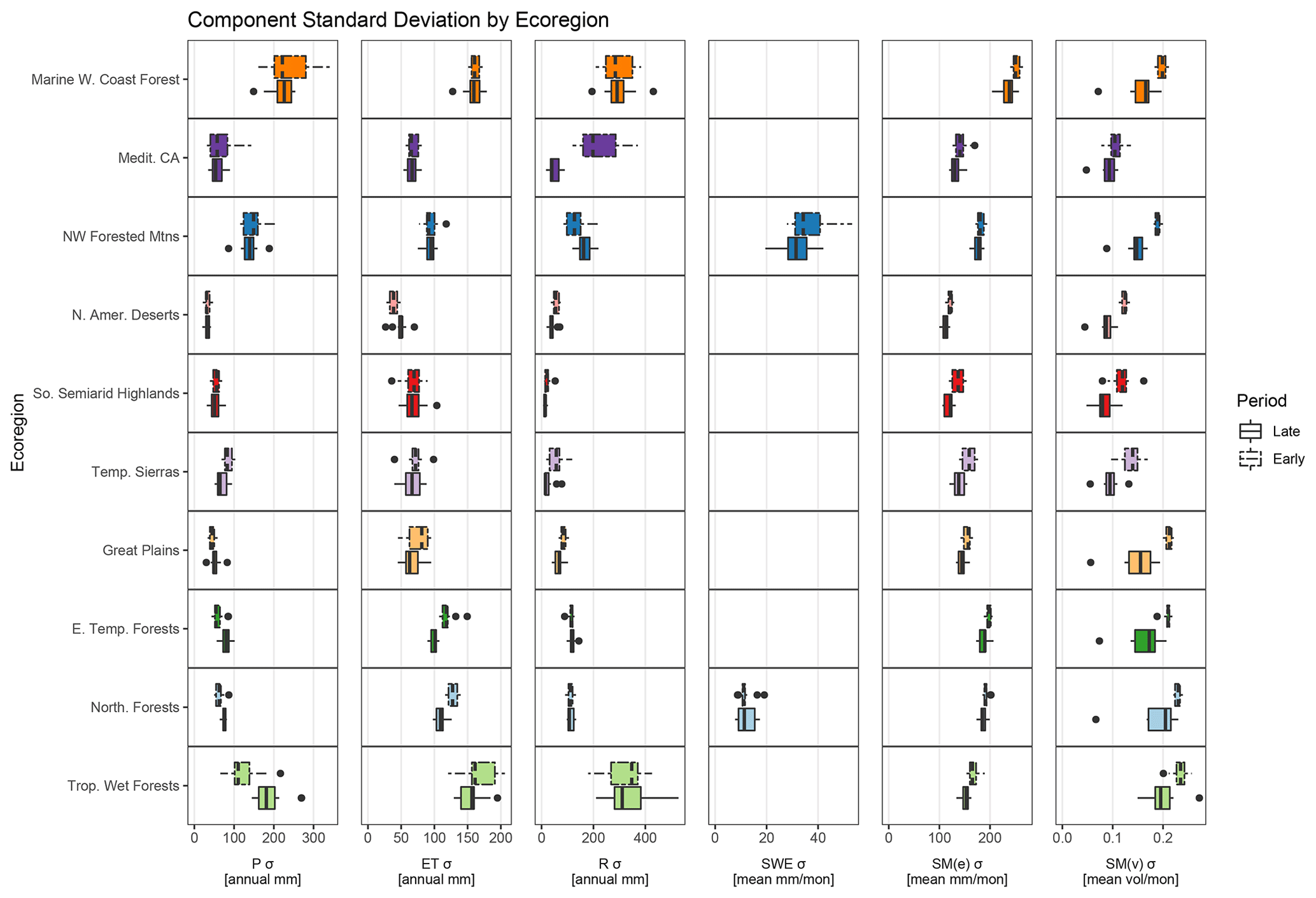
Figure B1 Box plots of annual standard deviation (σ) between component estimates at 10 ecoregions. σ distributions are subdivided into two periods, namely 1985–1999 and 2000–2014. Box lower limits, midlines, and upper limits represent the 25th, 50th (median), and 75th percentiles, respectively, of the associated data. Whiskers represent 1.5 times the interquartile range. Box colors denote ecoregions and correspond to map colors in Fig. 1. Components displayed are precipitation (P), evapotranspiration (ET), runoff (R), snow water equivalent (SWE), soil moisture in units of equivalent water depth (SM(e)), and soil moisture in units of volumetric water content (SM(v)).

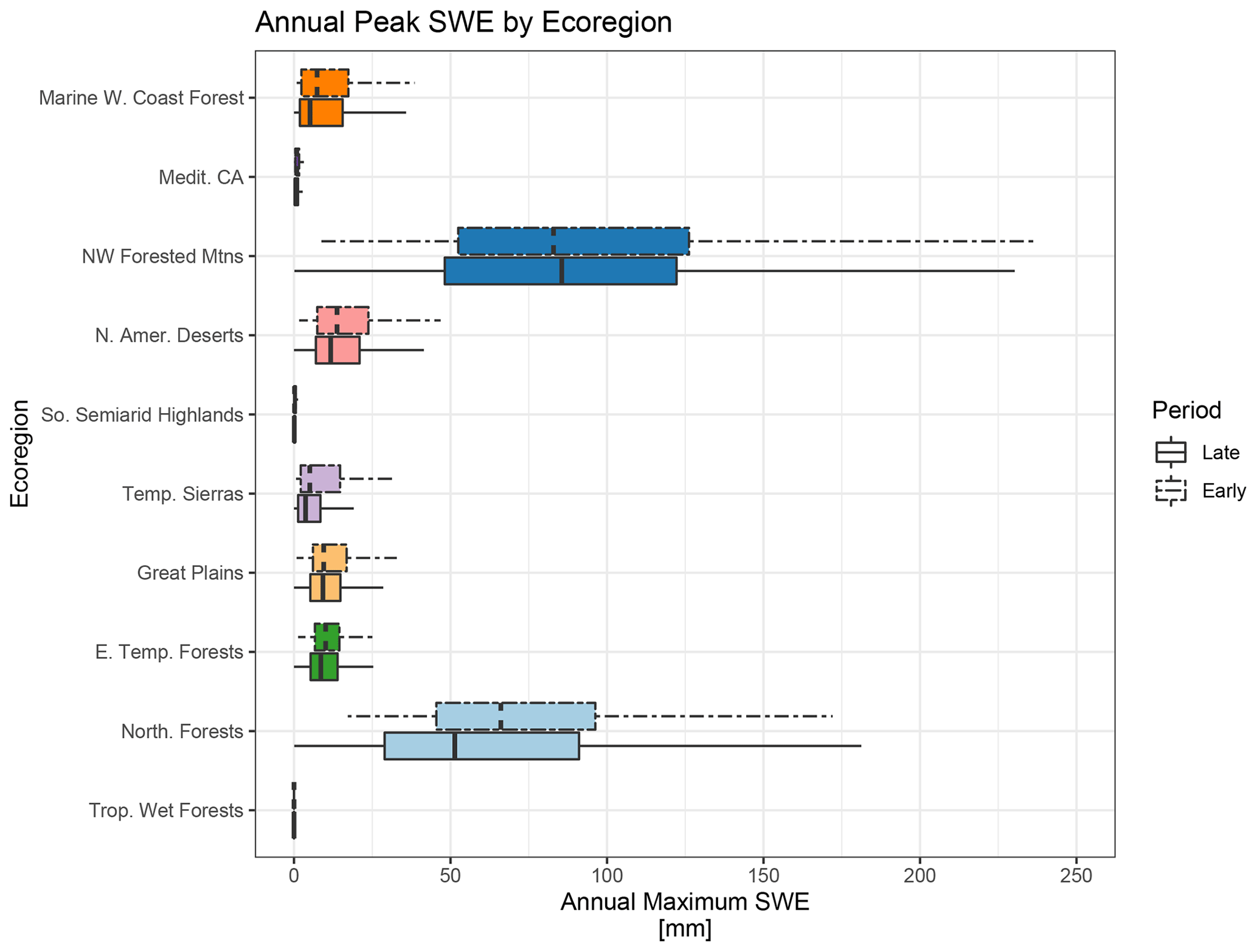
Figure B2 Box plot summarizing annual peak snow water equivalent (SWE) depths by ecoregion derived from the distribution of modeled estimates used in this paper. Box lower limits, midlines, and upper limits represent the 25th, 50th (median), and 75th percentiles, respectively, of the associated data. Whiskers represent 1.5 times the interquartile range.

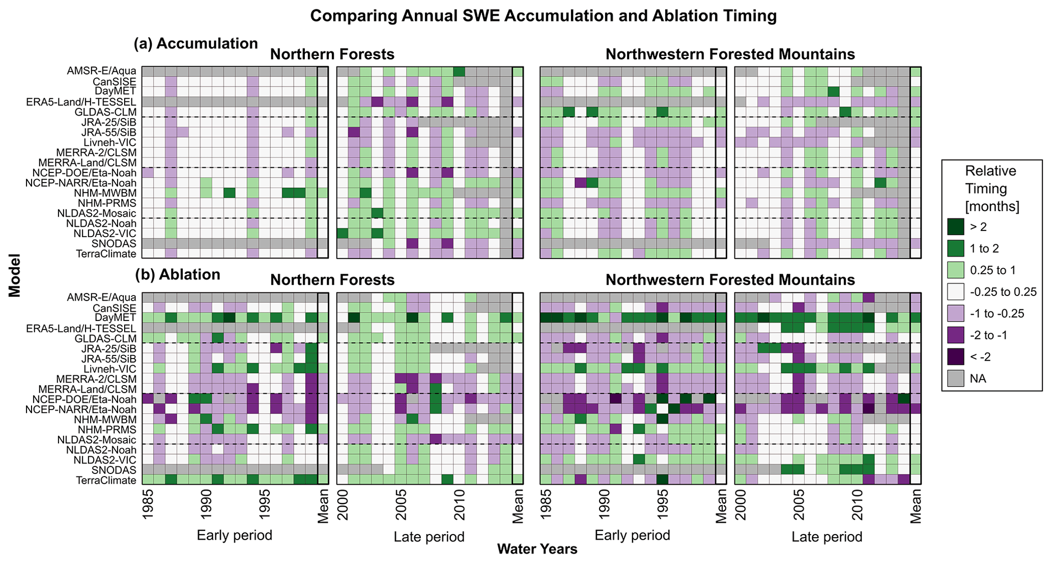
Figure B3 Heat maps showing the relative timing of the beginning of snow water equivalent (SWE) accumulation (a) and ablation (b) periods for two ecoregions from 1985 to 2014. Relative timing is the difference between the month of the beginning of a model's accumulation or ablation period and the mean of all other model's timing. The beginning of accumulation and ablation is defined as when the rate of change of SWE between months is greater than 1 mm per month or less than −1 mm per month, respectively.

Figure B4 Heat maps summarizing the annual relative timing values of SWE accumulation (accum.) and ablation from Fig. B3 for two ecoregions. Grid cells are colored by the percentage of years that have a positive relative timing (green) or by the percentage of years that have a negative relative timing (purple), whichever is greater.

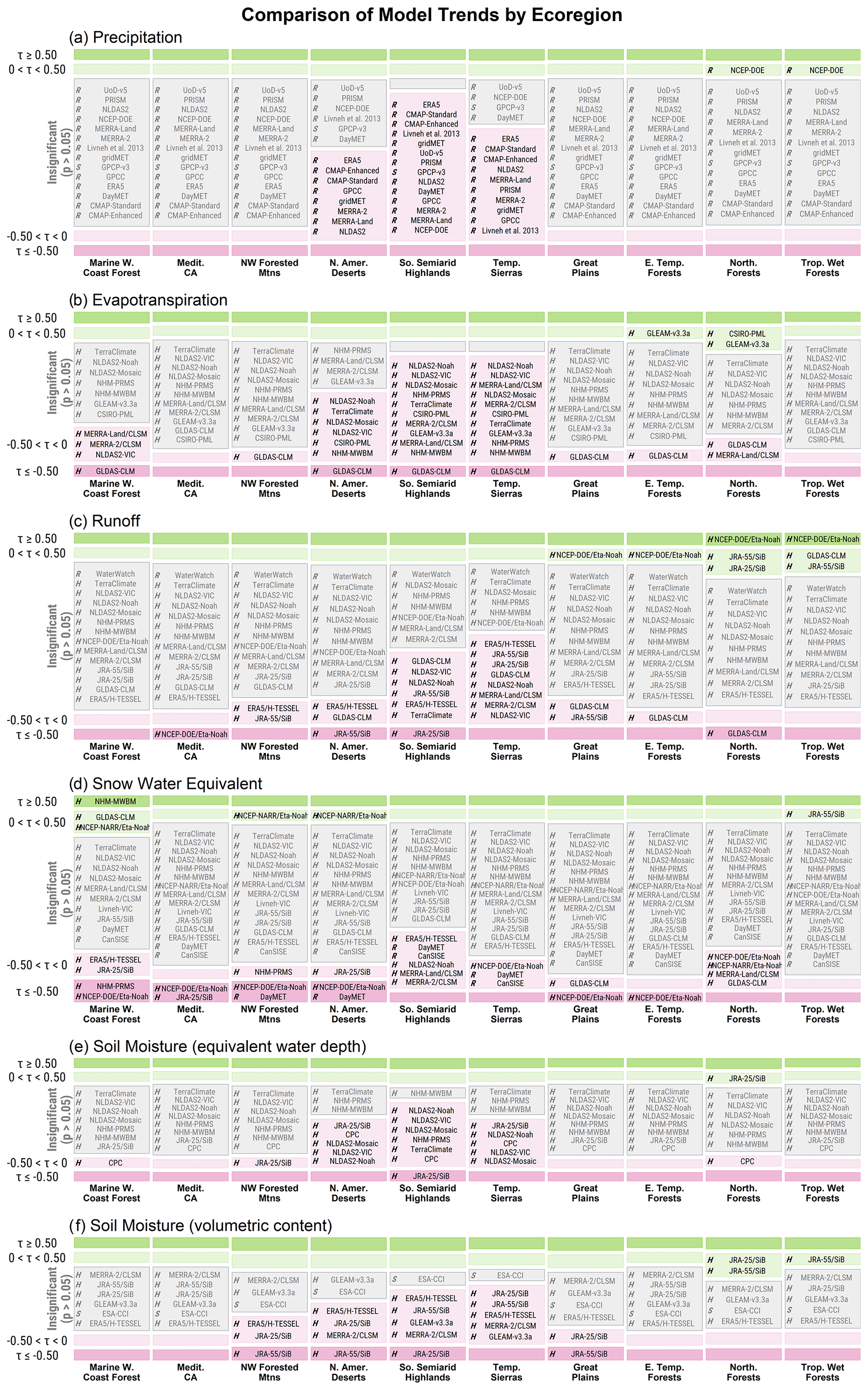
Figure B5 Binned distributions of interannual model trends from 1982 to 2010, measured with Mann–Kendall's tau (τ) for 10 ecoregions, for water balance components of precipitation, evapotranspiration, runoff, snow water equivalent, and soil moisture. Model names are binned into very positive (τ≥0.50; dark green), positive (0<τ<0.50; light green), negative (−0.50<τ<0; light purple), and very negative ($\mathit{\tau }\le -\mathrm{0.50}$; dark purple) significant trends, as well as an insignificant trend box (p>0.05; gray). Trend significance is assumed when the p value does not exceed 0.05 (p<0.05). Model categories are denoted with a single letter identifying either a hydrologic (H), reanalysis (R), or remote sensing (S) model.

Figure B6 Distribution of hydrologic model and reanalysis data set correlation against remote sensing products using Spearman's rho (ρ), provided by water budget component. Values of ρ are binned by >0.90, 0.50–0.90, <0.50, and statistically insignificant (p>0.05). Rectangles are color paired with their associated ecoregions (Fig. 1). Water budget components shown are precipitation (precip), evapotranspiration (ET), snow water equivalent (SWE), and soil moisture (SM).