the Creative Commons Attribution 4.0 License.
the Creative Commons Attribution 4.0 License.
 | 26 Mar 2021
Assessing the dynamics of soil salinity with time-lapse inversion of electromagnetic data guided by hydrological modelling
Mohammad Farzamian
Dario Autovino
Roberto De Mascellis
Giovanna Dragonetti
Fernando Monteiro Santos
Andrew Binley
Antonio Coppola
Irrigated agriculture is threatened by soil salinity in numerous arid and semi-arid areas of the world, chiefly caused by the use of highly salinity irrigation water, compounded by excessive evapotranspiration. Given this threat, efficient field assessment methods are needed to monitor the dynamics of soil salinity in salt-affected irrigated lands and evaluate the performance of management strategies. In this study, we report on the results of an irrigation experiment with the main objective of evaluating time-lapse inversion of electromagnetic induction (EMI) data and hydrological modelling in field assessment of soil salinity dynamics. Four experimental plots were established and irrigated 12 times during a 2-month period, with water at four different salinity levels (1, 4, 8 and 12 dS m−1) using a drip irrigation system. Time-lapse apparent electrical conductivity (σa) data were collected four times during the experiment period using the CMD Mini-Explorer. Prior to inversion of time-lapse σa data, a numerical experiment was performed by 2D simulations of the water and solute infiltration and redistribution process in synthetic transects, generated by using the statistical distribution of the hydraulic properties in the study area. These simulations gave known spatio-temporal distribution of water contents and solute concentrations and thus of bulk electrical conductivity (σb), which in turn were used to obtain known structures of apparent electrical conductivity, σa. These synthetic distributions were used for a preliminary understanding of how the physical context may influence the EMI-based σa readings carried out in the monitored transects as well as being used to optimize the smoothing parameter to be used in the inversion of σa readings. With this prior information at hand, we inverted the time-lapse field σa data and interpreted the results in terms of concentration distributions over time. The proposed approach, using preliminary hydrological simulations to understand the potential role of the variability of the physical system to be monitored by EMI, may actually allow for a better choice of the inversion parameters and interpretation of EMI readings, thus increasing the potentiality of using the electromagnetic induction technique for rapid and non-invasive investigation of spatio-temporal variability in soil salinity over large areas.
- Article
(9424 KB) - Full-text XML
- BibTeX
- EndNote


Soil salinization may be of a primary nature, when salt accumulation arises through pedogenetic processes, or of secondary origin, due either to abiotic factors such as excessive evaporation or seawater infiltration or resulting from human intervention, chiefly the use of saline water irrigation (Geeson et al., 2002). Approximately 20 % of irrigated land (45×106 ha) that produces one-third of the world's food is salt-affected (Shirvastava and Kumar, 2015), and it is estimated that soil salinity affects 1×10⁶ ha in the European Union, mainly in the Mediterranean countries (Maréchal, et al., 2008).
Effective agricultural management in many areas relies on a good understanding of the effects of irrigation on the spatial and temporal variability of soil salinity (Coppola et al., 2015). However, it is very difficult to assess soil salinity on a management scale using traditional methods. Soil salinity is traditionally assessed by measuring the electrical conductivity of a saturated soil paste (ECe) in the laboratory; however, this technique is labour-intensive, time-consuming and costly, given the large number of soil samples that need to be collected. Alternatively, time domain reflectometry (TDR), a non-destructive electromagnetic technique, can be used in the field for simultaneous measurements of water content, θ, and bulk electrical conductivity, σb (Coppola et al., 2011b). While the TDR method can provide accurate information from the local measurements, the measurement support volume of sensors is limited to a few centimetres; thus extension of the information to a large area can be problematic (Coppola et al., 2016; Gonçalves et al., 2017, Dragonetti et al., 2018).
The electromagnetic induction (EMI) technique is widely used as an alternative to traditional techniques for soil salinity assessment. It allows for rapid non-invasive, reliable and repeatable measurements at a smaller cost than traditional methods. This technique measures the soil electrical conductivity, which is primarily a function of soil salinity, soil texture, moisture content and cation exchange capacity; however, in a saline soil, the salinity is generally the dominant factor responsible for the spatio-temporal variability of soil electrical conductivity (Corwin and Lesch, 2005).
In the last few decades, EMI techniques have been used increasingly to estimate soil salinity from apparent electrical conductivity (σa) measurements (Lesch et al., 1995; Triantafilis et al., 2000; Corwin et al., 2006; Ganjegunte et al., 2014). σa is the weighted average of the soil electrical conductivity distribution in the soil volume. In order to obtain the depth distribution of σb from σa, a site-specific empirical calibration between σa and soil salinity measured at different depths can be applied by different approaches such as multiple regression (Triantafilis et al., 2000; Amezketa, 2006; Yao and Yang, 2010; Coppola et al., 2016), modelled coefficients (Slavich and Petterson, 1990), theoretical coefficients calculated with theoretical EMI depth response functions (Cook and Walker, 1992) or empirical-mathematical coefficients (Corwin and Rhoades, 1984).
Alternatively, to assess the distribution of σb with depth, σa data collected in the field can be modelled through an inversion process. Several inversion methods have been proposed to obtain the σb from the measured σa data, including the gradient-based inversion technique (Monteiro Santos, 2004; von Hebel et al., 2014; Schamper et al., 2012; Farzamian et al., 2015a) and probabilistic inversion (Jadoon et al., 2017; Moghadas, 2019; Shanahan et al., 2015). Recently, multi-coil EMI measurements and inversion algorithms have been widely used for mapping soil salinity and sodicity distribution in quasi 2D (e.g. Goff et al., 2014; Farzamian et al., 2019; Paz et al., 2019, 2020a, b) and 3D (e.g. Huang et al., 2017). However, the potential of this method in assessing temporal variability of soil salinity has not been fully explored. Several time-lapse inversion methods for direct-current resistivity methods have been developed. These include the ratio method (Daily et al., 1992), the difference inversion (LaBrecque and Yang, 2001) and, more recently, 4D space–time algorithms (Kim et al., 2009). A number of studies have also demonstrated how the use of time-lapse inversion algorithms can reduce the inversion artefacts (e.g. Hayley et al., 2011) and improve the quantitative investigations of geophysical monitoring (e.g. Farzamian et al., 2015b). However, the usefulness of the time-lapse inversion algorithms in modelling EMI data has not been attempted yet to assess soil salinity dynamics, and only few studies have been conducted to estimate soil water content changes (Huang et al., 2016; Whalley et al., 2017). In addition, a prerequisite for such an approach concerns the reliability of the inversion of the EMI result. In fact, inverting profile-integrated EMI data to obtain the vertical distribution of σb is an ill-posed problem, suffering from non-uniqueness (the problem has more than one solution) and instability (incomplete data and measurement errors can lead to large changes in the parameters; e.g. Tarantola, 1987). Ill-posedness is generally treated by regularizing the inverse solution. However, different regularization schemes and parameters can have a significant impact on the results (e.g. Dragonetti et al., 2018; Zare et al., 2020); thus, inversion results of EMI data are always affected by uncertainties, which can be minimized in case of prior information from the experiment.
In this direction, preliminary numerical simulations of the same hydrological processes to be monitored by an EMI sensor, by applying real boundary conditions measured during an EMI sensor monitoring campaign, may be especially helpful to figure out the response to be expected by the sensor and its variability in the space and time and may allow for a more rational choice of the EMI inversion parameterization. In other words, hydrological simulations may help provide a priori knowledge of “where the EMI inversion has to go”. In any case, this would require the actual distribution of the hydraulic properties along the transect or, more in general, in the field to be monitored by the EMI. One can immediately realize that this is quite utopian, especially when the area to be monitored is relatively large (as previously recalled in the case of EMI measurements). By contrast, it is more common that, for the study area, one has the statistical distribution of hydraulic properties available. Thus, the statistical distribution of the hydraulic properties may be used for generating synthetic (but realistic in a probabilistic view) equiprobable realizations of the physical conditions the EMI sensor will potentially experience during the monitoring, which may be used for addressing the inversion of EMI reading.
The main objective of this paper is to propose an approach to improve the parameters' optimization and the constraints in the time-lapse EMI inversion using soil water and solute modelling. In the paper we will show how the synthetic tests may be used to guide the optimization of inversion parameters and understanding of the impact of solute concentration and water content variations on EMI σa readings.
The key features of this study are (i) performing a controlled irrigation experiment, allowing for the simulation of the spatial and temporal variability of soil salinity during the irrigation experiment; (ii) monitoring of σa using the multi-coil CMD Mini-Explorer EMI sensor which takes σa measurements over six different depth sensitivity ranges; (iii) running numerical simulations using a physically based hydrological model to study how well the EMI survey and time-lapse inversion can resolve the σb distribution in space and time in our experimental set-up and to infer the best inversion parameters; (iv) inverting time-lapse field σa to map the spatio-temporal variability of σb and to interpret them in terms of concentration distributions over time.
2.1 Experimental set-up
The experiment was carried out at the Mediterranean Agronomic Institute of Bari in south-eastern Italy. The soil is classified as Colluvic Regosol, consisting of silty loam material of an average thickness of 0.7 m lying on fractured calcarenite bedrock. Figure 1 shows the experimental set-up, consisting of four experimental plots each of 30 m length and 3.6 m width, equipped with a drip irrigation system, with nine irrigation dripper lines placed 0.40 m apart, and characterized by an inter-dripper distance of 0.20 m. Pressure self-compensating drippers were used, and the emission uniformity was over 90 %. The soil was bare during the experiment period to avoid the effect of root uptake on the interpretation of the results. The four experimental plots were irrigated with water at four different salinity levels, experimental plot 1: water at 1 dS m−1 (hereafter referred to as P1); experimental plot 2: water at 4 dS m−1 (hereafter P2); experimental plot 3: water at 8 dS m−1 (hereafter P3); experimental plot 4: water at 12 dS m−1 (hereafter P4).
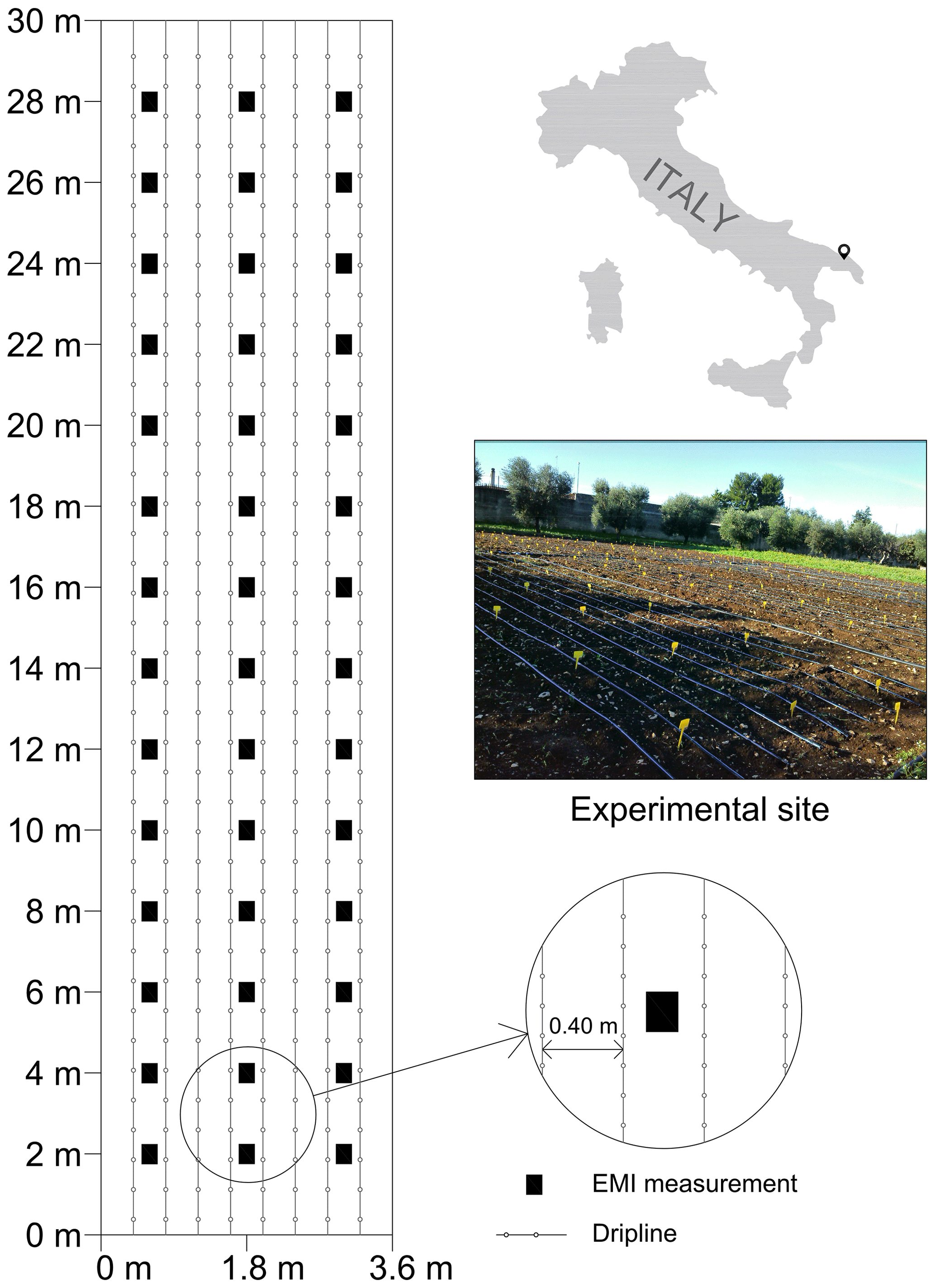
Figure 1A schematic display of the experimental set-up. Four experimental plots were designed equally and irrigated with the same amount of water at four different salinity levels.
The soil–bedrock depth was measured at 40 points by augering, and the resulting spatial distribution is shown in Fig. 2. An apparent variability in the depth to bedrock was revealed, which may have significant impacts on the spatio-temporal distribution of water and solute concentration.
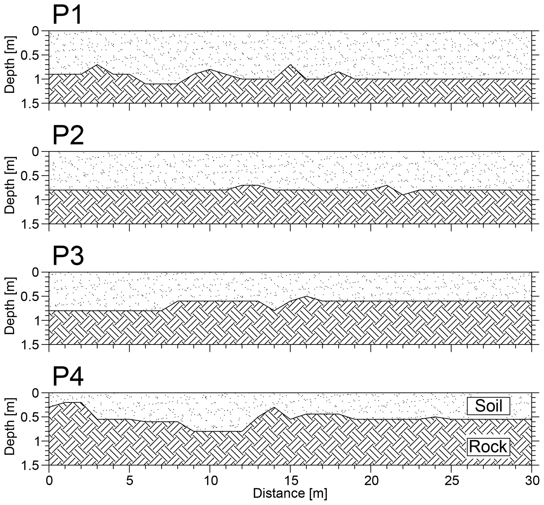
Figure 2Measured spatial distribution of the soil depth along four experimental plots, P1, P2, P3 and P4.
Irrigations were started on 30 September 2016, and all experimental plots were irrigated 12 times until 21 November 2016 with the same amount of water and delivering day. Water salinity was induced by adding calcium chloride (CaCl2) to well water with a salinity of about 1 dS m−1. Each saline application was of about 18 mm, with a Cl− concentration of about 0.1 mmol cm−3. The volumes of supplied water were calculated according to the differences between two consecutive level measurements in a Class A evaporimeter. The details of irrigation events and precipitation information are given in Fig. 3. EMI measurements were taken four times during the experiment period in each experimental plot along three transects, 1.2 m apart and at 2 m spacing, as shown in Fig. 1. All measurements were taken 1–3 d after the irrigations, allowing relatively time-stable water contents to be assumed at each site throughout the monitoring phases.
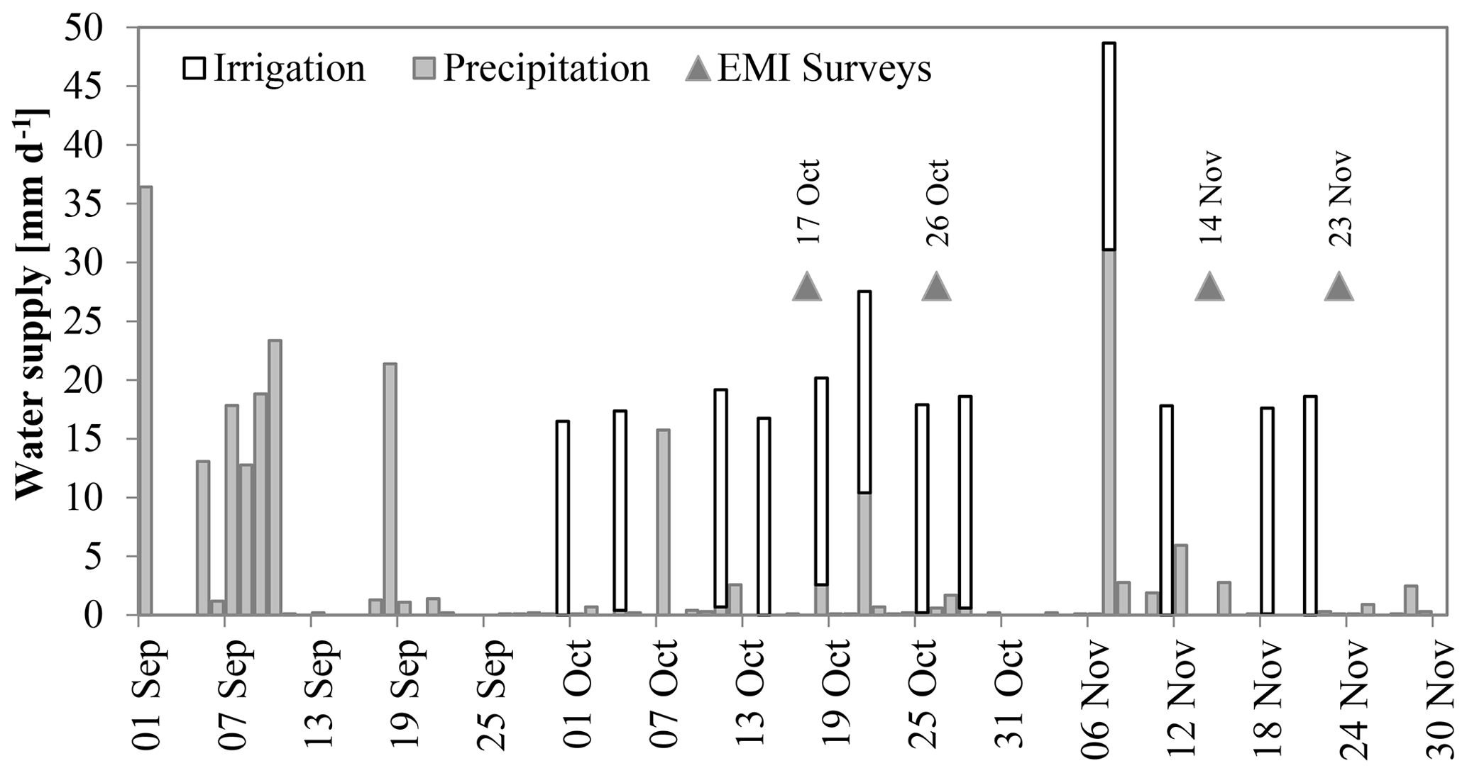
Figure 3The details of irrigation events and precipitation information during the experiment. The dates of EMI measurements are marked with triangles.
2.2 EMI analysis
2.2.1 Characteristics of the EMI sensor
σa data were collected using a CMD Mini-Explorer device (GF Instruments, Brno, Czech Republic). The characteristics of this device make it especially suitable for monitoring electrical conductivity at relatively shallow depths. The CMD Mini-Explorer was used to measure σa in VCP (vertical coplanar, i.e. horizontal magnetic dipole configuration) mode and then HCP (horizontal coplanar, i.e. vertical magnetic dipole configurations) mode by rotating the probe 90∘ axially to change the orientation from VCP to HCP mode. The probe has three receiver coils with 0.32 (ρ32), 0.71 (ρ71) and 1.18 (ρ118) m distances from the transmitter coil and operates at 30 kHz frequency. With the largest coil spacing, the instrument has an effective depth investigation of 1.8 m in the HCP mode and 0.9 m in the VCP mode.
2.2.2 Electromagnetic forward model
The electromagnetic forward modelling is solved by applying the full solution of the Maxwell equations to calculate the σa responses of a 1D model. The response of a layered media (secondary magnetic field) excited by a small horizontal transmitter loop above the ground surface can be expressed in terms of the Hankel transform (Zhang et al., 2000):
where M is the moment of the transmitter loop emitting at an angular frequency ω, and zs and zr are the heights of the transmitter and receiver loops, respectively. r is the transmitter–receiver distance, and Jo is the Bessel function of first kind and order zero.
The kernel function RTE is defined as
where Z0 is the intrinsic impedance of free space, and Z1 is the input impedance at the first layer calculated by a recursive procedure. Similar equations can be written for vertical coplanar loops. In such cases the secondary magnetic field is
where J1 is the first-order Bessel function.
σa (mS m−1) is usually calculated assuming the low induction number (LIN) approximation using the formula
where μ0 is permeability of free space, and Q denotes the out-of-phase component of the secondary to primary magnetic field coupling ratio.
2.2.3 Time-lapse inversion
With the time-lapse inversion, one seeks to calculate the temporal variation of the conductivity along a transect. The quasi-2D inversion algorithms based on Monteiro Santos (2004) with a modification of the algorithm proposed by Kim et al. (2009) were used in this study. The problem is resolved in both algorithms iteratively starting from a uniform model. Two different levels of constraints, S1 and S2, were applied. In the S1 option, the corrections to the model parameters at each iteration are calculated by solving the system of equations
In the S2 option, the corrections of the parameters at each iteration are calculated solving the equations
where δp is the vector comprising corrections of the parameters (logarithm of conductivities, pj) of an initial model; po refers to a reference model; b is the vector containing the differences between the logarithm of the observed and calculated apparent conductivities. J is the Jacobian matrix with elements given by . λ is a Lagrange multiplier and determines the amplitude of the parameter corrections in the space domain, and the regularization matrix C stores the coefficients of the spatial roughness of the model parameters at time t, which is defined as
where the elements of matrix C are 1 or −4 according to the position of the neighbours. α is a parameter that determines the amplitude of the parameter corrections in the time domain, and M is a square matrix that accounts for the temporal continuity of the model parameters.
The elements of matrix M are defined in terms of models at time t−dt and t+dt. The model misfit is calculated using the following equation:
where N is the number of apparent conductivity value, with and representing observed and calculated σa, respectively.
In this algorithm, two regularizations are imposed in both space and time domains. Consequently, the spatial and temporal Lagrangian multipliers have to be optimized. The spatial Lagrangian multiplier (λ) controls the relative importance of spatial model smooth and data-response misfit and decreases gradually during the inversion process to resolve more detailed model parameters. A larger λ tends to generally produce a model with a larger misfit error but smooth variation of conductivity values. A larger λ is usually acceptable if the soil conductivity changes in a smooth manner and allows a model to be produced that is reasonably more realistic. In contrast, a smaller λ is usually required when sharper soil conductivity changes are expected in order to resolve the sharp boundaries. A suitable λ value is usually determined empirically based on the expected distribution of σb and by performing inversions with different values. The second regularization, the temporal Lagrangian multiplier (α), is the temporal damping factor that gives the weight for minimizing the temporal changes in the conductivity along the time axis. α is a constant value and is defined by the similarity of the two consecutive reference times. The larger the α value, the more similar the reference models are that result from the inversion; a value of zero means no temporal constraints are applied (i.e. a traditional non-time-lapse inversion). The misfit function in this algorithm is the square root of the sum of the squares of the differences divided by the number of the measurements and is expressed in millisiemens per metre (mS m−1).
2.3 Synthetic experiment
2.3.1 Hydraulic properties' dataset
A large dataset of hydraulic properties was already available from the experimental site, which was obtained by previous laboratory and field hydraulic characterizations carried out during several measurement campaigns (e.g. Coppola et al., 2011a, b, 2013, 2015). A total of 70 soil samples were collected from the Ap and Bw horizon in the experimental farm. Saturated hydraulic conductivity, K0, and water retention experimental data were measured in the laboratory by the falling head permeameter (Reynolds and Elrick, 2003) and tension table method (Dane and Hopmans, 2003), respectively. The water retention data were fitted to the van Genuchten model (van Genuchten, 1980):
where Se (–) is the effective saturation, α (cm−1), n (–) and m (–) are shape parameters, and θ0 (–) and θr (–) are the saturated and residual water content, respectively.
The hydraulic conductivity was estimated by the van Genuchten–Mualem model (van Genuchten, 1980), with :
where K0 is the saturated hydraulic conductivity, Kr (–) is the relative hydraulic conductivity and τ (–) is a parameter which accounts for the dependence of the tortuosity and the correlation factors on the water content.
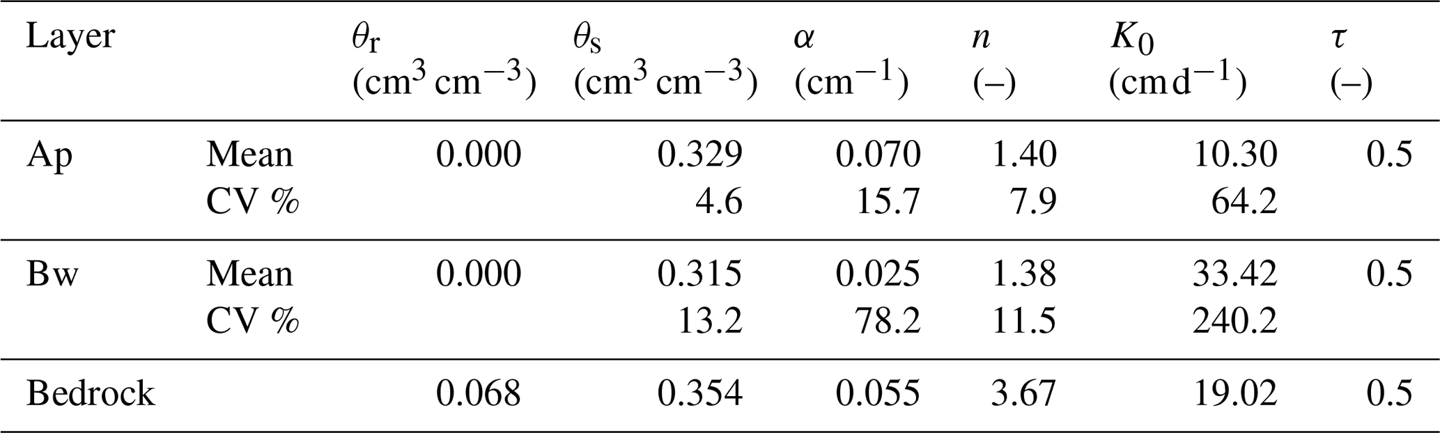
Due to the different hydrological behaviour between the laboratory and the field (Kutilek and Nielsen, 1994), the laboratory-derived curves were scaled to the field curves by applying the procedure described in Basile et al. (2003, 2006). Statistics of the parameters are reported in Table 1. The data in the table indicate a larger variability of the hydraulic properties of the Bw horizon, compared to the Ap horizon. This is probably due to the frequent roto-tillage of the Ap horizon, inducing significantly greater homogeneity of this soil layer. Actually, even the apparent larger variability of the K0 for the Ap horizon is much lower than the variability reported in the literature, which is generally characterized by a coefficient of variation (CVs) much larger than 100 % (Kutilek and Nielsen, 1994; Mallants et al., 1996; Coppola et al., 2011a) and may even reach values of 450 % (Carsel and Parrish, 1988). The hydraulic properties' parameters for the bedrock were those determined on the same type of bedrock by Caputo et al. (2010, 2015).
Table 1Statistics (mean and coefficient of variation, CV) of the hydraulic property parameters of the two soil layers and bedrock.
2.3.2 Synthetic hydrological simulations
2D numerical simulations of the infiltration and redistribution process were carried out using Hydrus 2D/3D software (Šimůnek et al., 2016), by introducing the actual boundary conditions imposed during the experiment to (i) gain an insight into the spatio-temporal distribution of water and solute concentration during the experiment period, prior to interpreting the field EMI data, and to (ii) optimize the EMI inversion parameters. The Richards equation and advection–dispersion equation were used to simulate water flow and solute transport, respectively. The distributions of the hydraulic parameters (see Table 1) were used to generate several synthetic transects, with variable hydraulic properties and depth to bedrock (electrically resistive layer), in order to simulate different distributions of water contents, solute concentrations and soil depths and to explore their role in the variability of the σa response. Each synthetic transect consisted of an assembly of 30 interacting soil columns, each with its own hydraulic properties and depth to bedrock. Each of the 30 soil profiles included three horizons: Ap (0–15 cm), Bw and bedrock. The Bw and bedrock thickness changed in each soil profile according to the depth of the soil–bedrock interface. For hydraulic properties, the transect variability was assumed to be characterized by the variability of the parameters θ0, α, n and K0. The hydraulic properties and depth to bedrock were assigned randomly to each soil column by using the statistical distribution of each parameter (see Table 1). Statistical tests showed that θ0 and n were normally distributed, K0 and α log-normally distributed and depth to bedrock uniformly distributed. The means and the covariance matrix for θ0, log K0, log α, and n were computed. Due to continuous ploughing and other tillage practices (see Sect. 2.1), the Ap horizon is rather homogeneous, and therefore only the hydraulic parameters of the horizon Bw were considered to vary stochastically. The hydraulic parameters of both Ap horizon and bedrock were fixed to their average values.
A total of 20 synthetic transects with 30 random vectors of the four parameters (θs, α, n and K0) were produced from the correlated multivariate distribution by generating a vector x of independent standard normal deviates and then applying a linear transformation of the form , where m is the desired vector of means, and L is the lower triangular matrix derived from the symmetric covariance matrix V=LLT decomposed by Cholesky factorization (Carsel and Parrish, 1988). θr was set to zero for all simulations. For solute transport, a longitudinal dispersivity of 2 cm was assumed according to a previous experiment carried out in the same field (Coppola et al., 2011b). Transverse dispersivity was assumed to be one-tenth of the longitudinal dispersivity (Mallants et al., 2011). The simulation time – according to the field experiment data – included a period of 91 d from 1 September to 30 November 2016 in which 12 irrigations were applied (a total of 210 mm), the water with an electronic conductivity (EC) of 12 dS m−1 (each one of about 18 mm with a Cl− concentration of about 0.1 mmol cm−3). The level of 12 dS m−1 was considered because spatial and temporal variabilities of σb were expected to be larger and more apparent due to greater salinity changes. Potential evapotranspiration was estimated by a local agrometeorological station; irrigation fluxes and Cl− concentration in the irrigation water were considered to be top boundary conditions. Free drainage was assumed at the lower boundary (). The initial soil water content value was set to 0.25 cm3 cm−3, based on the field measurements by a TDR probe, and the initial Cl− concentration was set equal to zero.
It is worth noting that the use of synthetic transects does not aim to address the overall spatial variability of soil properties potentially observable in the investigated field but to randomly select a reasonable number of different scenarios to better understand how solute concentration and water content changes during the experiment influence σb distribution. They also help to identify a proper regularization strategy to invert measured σa data in the field. In this sense, the number (20) of transects is a trade-off between the need of accounting for the possible heterogeneity of the field and the computational challenge of carrying out too many synthetic data inversions.
For each generated transect, numerical simulations produced distributions of water contents and Cl− concentrations.
2.4 Site-specific calibration
The water content and Cl− concentration distributions were converted to bulk electrical conductivity (σb) distributions by using the model proposed by Malicki and Walczak, 1999:
where εb (–) is the dielectric constant, which is related to the water content, and σw (dS m−1) is the electrical conductivity of the soil solution. The latter was obtained by using a linear relationship C–σw for solutions at different concentrations of calcium chloride.
The parameters for the Malicki and Walczak model were calibrated through a laboratory experiment. Specifically, εb and σb for different values of σw were simultaneously measured on reconstructed soil samples values using TDR probes. For this purpose, four PVC cylinders (8 cm in diameter and 15 cm height) were filled with air-dried soil, reaching a dry bulk density of about 1.1 g cm−3, imitating the field condition. Each soil sample was wetted by adding 10 mL of CaCl2 solution at a specified electrical conductivity: 1, 2, 4 and 6 dS m−1, respectively. The cylinders were covered by 0.05 mm plastic foil before the measurement in order to avoid evaporation and to equilibrate with the air temperature of 20 ∘C. The procedure was repeated 16 times for each soil sample to measure soil water content values ranging from air-dried to near saturation. For each wetting step, the measurements of θ and σb were carried out using TDR three-wire probes (10 cm long with a rod diameter of 0.3 cm and rods spaced 1.2 cm) vertically inserted in the soil columns. The following parameters of Eq. (10) were obtained: a=3.6 dS m−1; b=0.11.
2.5 Schematic view of the approach used in the paper
The logical sequence of the different steps used in the proposed approach is described in Fig. 4.
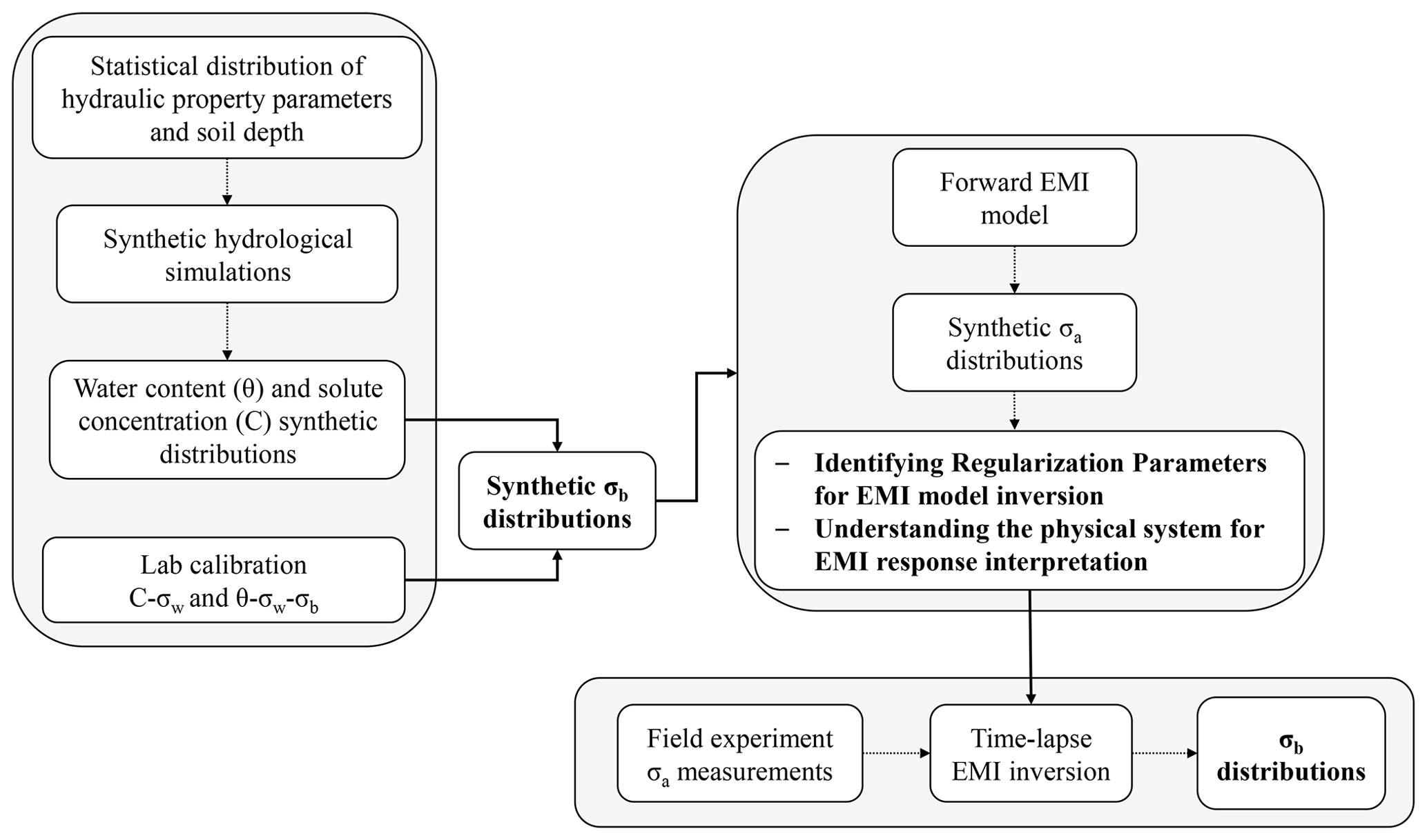
Figure 4Flow chart of the applied procedure, with the key steps in bold. The procedure is explained in detail in the text.
-
Starting from the statistical distribution of the hydraulic properties and the physical characteristics of the system under study (the latter limited to only depth to the bedrock, in this specific case), as described in Sect. 2.3.1, several synthetic transects are generated, each accounting for some of the variability in terms of hydraulic properties and physical characteristics that the EMI sensor potentially experiences during the monitoring.
-
Hydrological simulations for each of these synthetic transects are thus carried out, each producing synthetic distributions of both water contents and solute concentrations, as described in Sect. 2.3.2, which, in turn, are converted to as many synthetic distributions of σb by using a specifically developed calibration relationship, discussed in Sect. 2.4.
-
These σb distributions are used in a forward EMI modelling procedure (see Sect. 2.2.2.) to generate synthetic σa data for all the synthetic transects considered.
-
The σa, θ and σw (C) distributions are used to guide the inversion of EMI readings obtained during real monitoring campaigns carried out in the physical system under study in two different (but related) ways: (i) to have a priori knowledge of where a measured EMI reading may come from (e.g. at a given time, a measured σa distribution could come from the depth of the water or solute propagation front, from the depth to the bedrock or from water accumulation at the soil–bedrock interface); (ii) to identify the optimal regularization parameters, discussed in Sect. 2.2.3, to be used in the inversion model of the real EMI data, by looking for example to the parameter value, allowing for satisfactory results for most of the synthetic transects. For the latter purpose, we compare different inversion parameter combinations in terms of correlation (correlation coefficient, R), precision (mean square error, RMSE) and bias (mean error, ME) between the simulated and modelled σb.
-
Finally, with all this information at hand, one is ready to look at the real EMI datasets, by producing more realistic σb distributions which can now be seen with much more confidence compared to cases where EMI inversion has to be carried out without any prior information from the experiment and, thus, producing less interpretable and more uncertain σb distributions.
The Results and discussion section below will show the application of the approach to the system under study, with an analysis of the real EMI data carried out only in the final phase, when all the information needed are available to guide the inversion of the real EMI data and interpretation of the obtained models.
3.1 Synthetic spatio-temporal distributions of solute water content and solute concentration
This section shows how the synthetic simulations described in Sect. 2.3.2 can be used to analyse the sensitivity of the EMI response to both the hydrological behaviour and physical characteristics of the system under study.
As an example, Fig. 5 depicts the depth to the bedrock for one of the synthetic transects described in Sect. 2.3.2. For the same transect, Fig. 6 shows, for 4 selected days, the spatial distribution of water content obtained from the Hydrus 2D/3D simulations with irrigation water at 12 dS m−1. The soil shows very high values of water content on the selected days. This is because the water was supplied to the soil only 1–3 d before the selected days. On the other hand, lower values were obtained at larger depths within the bedrock. The water content distributions show a significant lateral heterogeneity, while the temporal variations are very small. The spatial variations of water content distribution can be partly explained by the variability of the hydraulic properties. However, soil depth proved to be the dominant factor in determining water content lateral variability. In fact, high inverse correspondence of soil depth with water content is revealed in the vertical profiles where bedrock is superficial (e.g. profiles 3, 4 and 5) or deep (i.e., profiles 19, 20 and 21). The correlation between soil depth and water content averaged along each profile is very high (r=0.88) for the four dates, thus confirming that the depth of the bedrock is the main factor governing the water distribution.
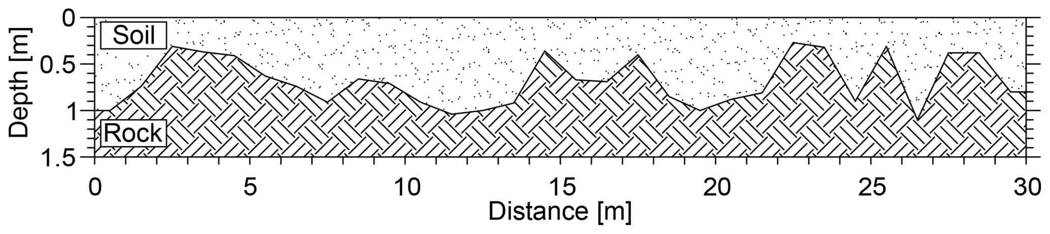

Figure 6Soil water content distribution simulations for the selected scenario: (a) 17 October, (b) 26 October, (c) 14 November and (d) 23 November 2016.
In terms of the temporal variations, the water content distribution did not change significantly, and the average soil water content of the whole soil profile was found to be similar on the selected dates, with an average in the range 0.20–0.22 cm3 cm−3 and a standard deviation of 0.02 cm3 cm−3. This was expected as the experimental field was irrigated regularly, and the four selected dates refer to approximately the same time after an irrigation application (1–3 d). However, small differences of water content may be observed near the soil surface, which may well be explained by the evaporation process taking place during the 1–3 d after irrigation and mostly involving the shallower soil layer. For example, the near surface shows higher water content (i.e. 0.25–0.30 cm3 cm−3) on 26 October because the irrigation took place 1 d before on 25 October. On the other hand, lower water content is evident in the near surface on 17 October due to a 3 d gap between the water irrigation on 14 October and the simulation date. Figure 7 shows the spatio-temporal distribution of Cl− concentration obtained for the same synthetic transect of Fig. 6. Compared to the water content, Cl− concentrations show a significantly greater evolution over time, with a slow and steady Cl− concentration increase along the soil profile due to the 12 injections of saline water. On average, the front of chloride deepens slowly at a fairly constant rate but with a lateral variability, which is related to the lateral variability of water contents and hydraulic properties. The lateral variability is quite low on the first days of solute applications and becomes evident only when the solute migrates deeper into the soil profile. The lateral variability of Cl− concentration is mainly related to the depth to bedrock, as can be immediately observed by comparing the solute distributions and the transect morphology shown in Fig. 5. The depth of the soil–bedrock interface as well as soil hydraulic properties condition the spatial distributions of water contents, which, in turn, influence the Cl− concentration distribution.
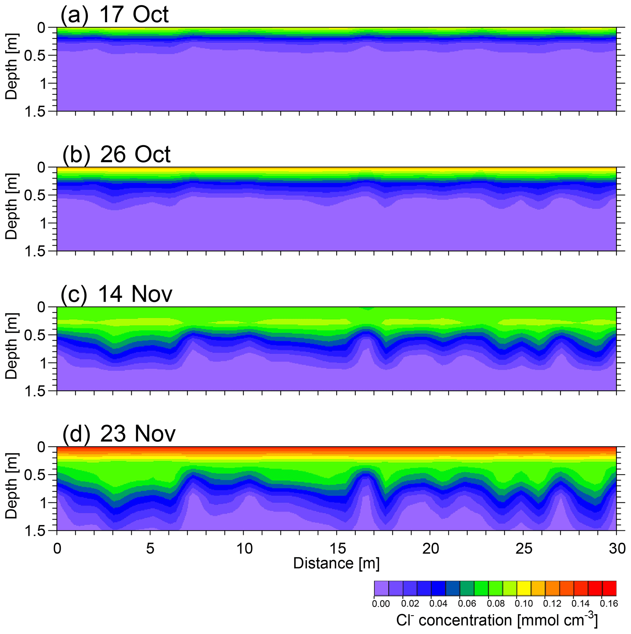
Figure 7Soil Cl− concentration distribution simulations for the selected scenario: (a) 17 October, (b) 26 October, (c) 14 November and (d) 23 November 2016.
3.2 Simulated spatio-temporal distribution of σb
Figure 8 shows the spatio-temporal distribution of σb for the same synthetic transect, obtained by converting water contents and solute concentrations by applying Eq. (10). Figure 8 shows a resistive zone beneath a conductive zone. The conductivity of the resistive zone varies slightly spatially and temporally; however the conductivity of this zone is generally within 25 mS m−1. The resistive zones in the maps correspond to the bedrock in the study area (see Fig. 5). The conductivity of the upper layers changes significantly both spatially and temporally from an average conductivity of 50 mS m−1 on 17 October to more than 100 mS m−1 on 23 November. The time evolution of the conductive zone is evident and, as the water content does not change significantly over time, is mostly related to the chloride propagation during the simulation. The lateral variation at any time, by contrast, is largely ascribable to bedrock topography.
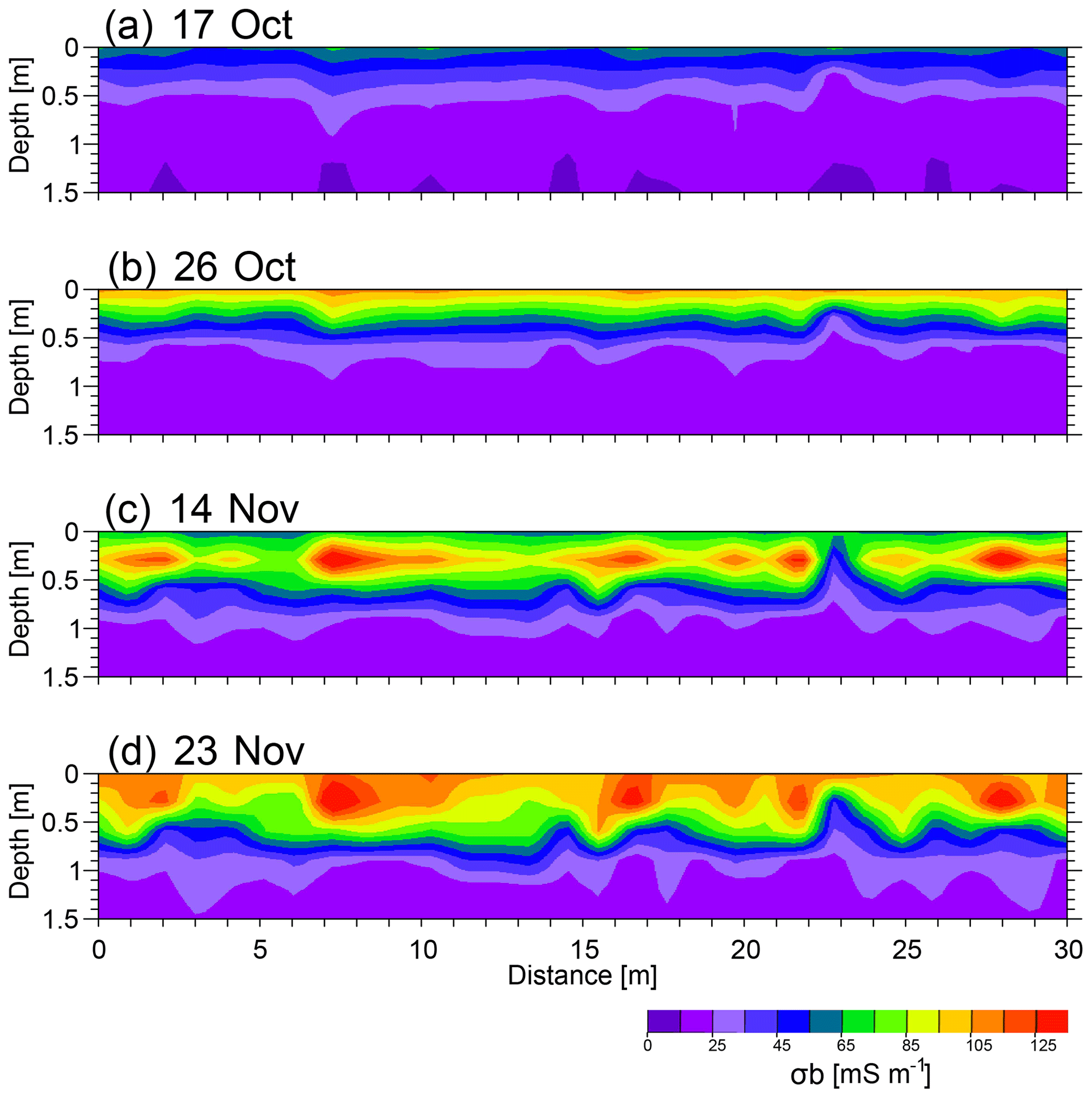
Figure 8σb distribution simulations for the selected scenario: (a) 17 October, (b) 26 October, (c) 14 November and (d) 23 November 2016.
3.3 Time-lapse synthetic σa data
The spatio-temporal distribution of σb shown in Fig. 8 was used to generate the time-lapse synthetic σa data. The generated σa data for the model obtained on 23 November (see plot d in Fig. 8) are shown in Fig. 9. Profile ρ32 shows the greatest σa values in each orientation, while the minimum σa was recorded on profile ρ118, indicating a conductive zone over a resistive zone, which is expected from the model shown in Fig. 8d. In addition, significant lateral σa change is evident along the transect, with strongest fluctuations in ρ32 in both orientations. This is because of the strong lateral σb variations at the near surface due to the saline water infiltration and heterogeneity of the subsurface. The general behaviour of the synthetic σa data suggests that the field data might have strong lateral σa changes along the transect, and a careful processing of data is required (e.g. filtering of σa data should be avoided).
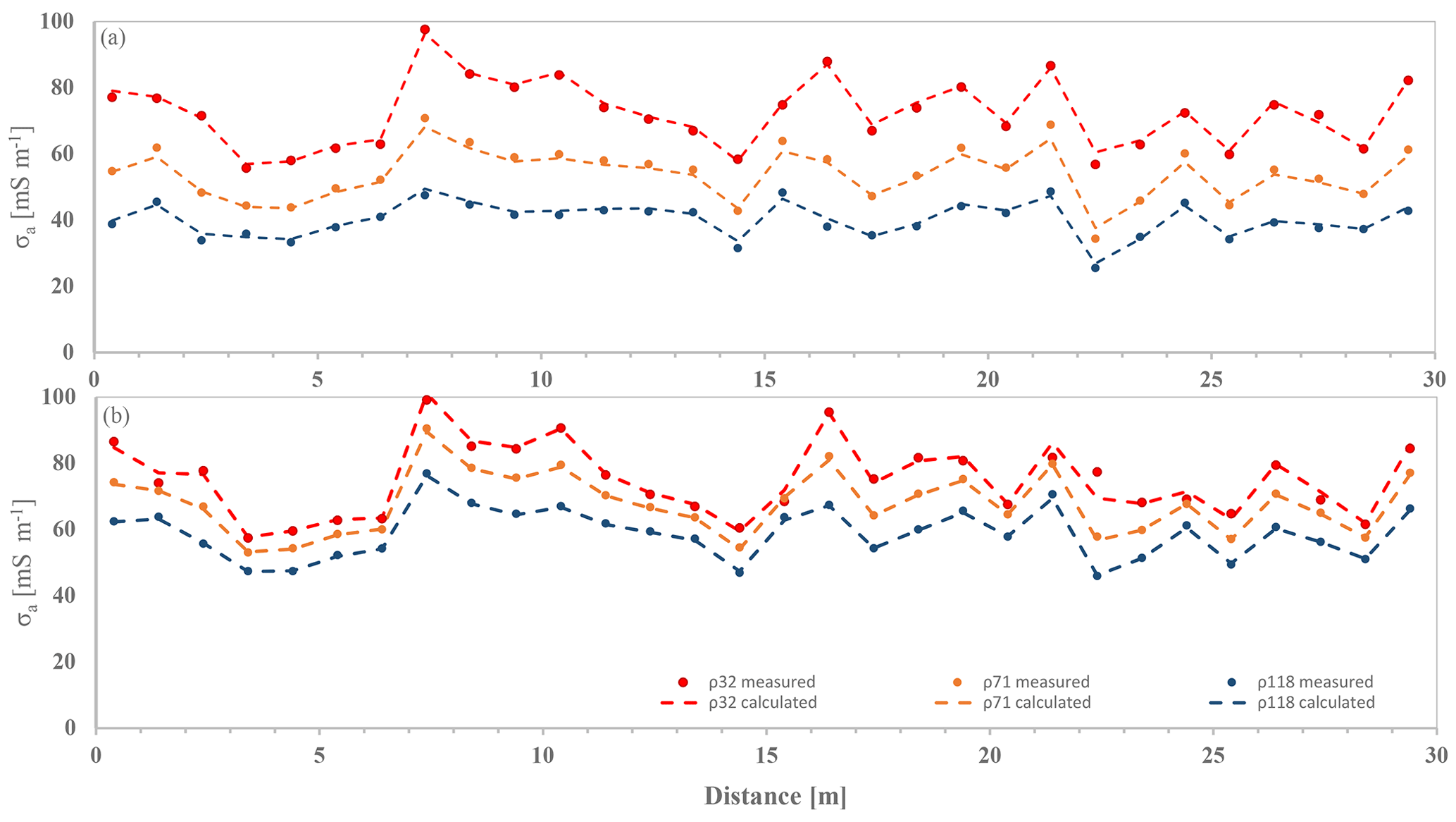
Figure 9σa data generated from the forward calculation of the σb distributions on 23 November, shown in Fig. 8d. (a) HCP-mode and (b) VCP-mode configurations are displayed.
3.4 Optimizations of the inversion parameters
In this section we show how well the developed inversion method can resolve the σb distribution from generated synthetic σa distribution. Firstly, we investigated the influence of the spatial smoothing parameter (λ) and the inversion algorithm S1 (Eq. 5) and S2 (Eq. 6) in the Supplement in resolving the σb distribution. In this regard, the generated σa data were inverted using both S1 and S2 and different values of λ in the 0.01 to 10 range. Figure 10 shows an example of the σb distribution models after inverting the synthetic σa data presented in Fig. 9 This example was selected due to the larger lateral and vertical contrast.
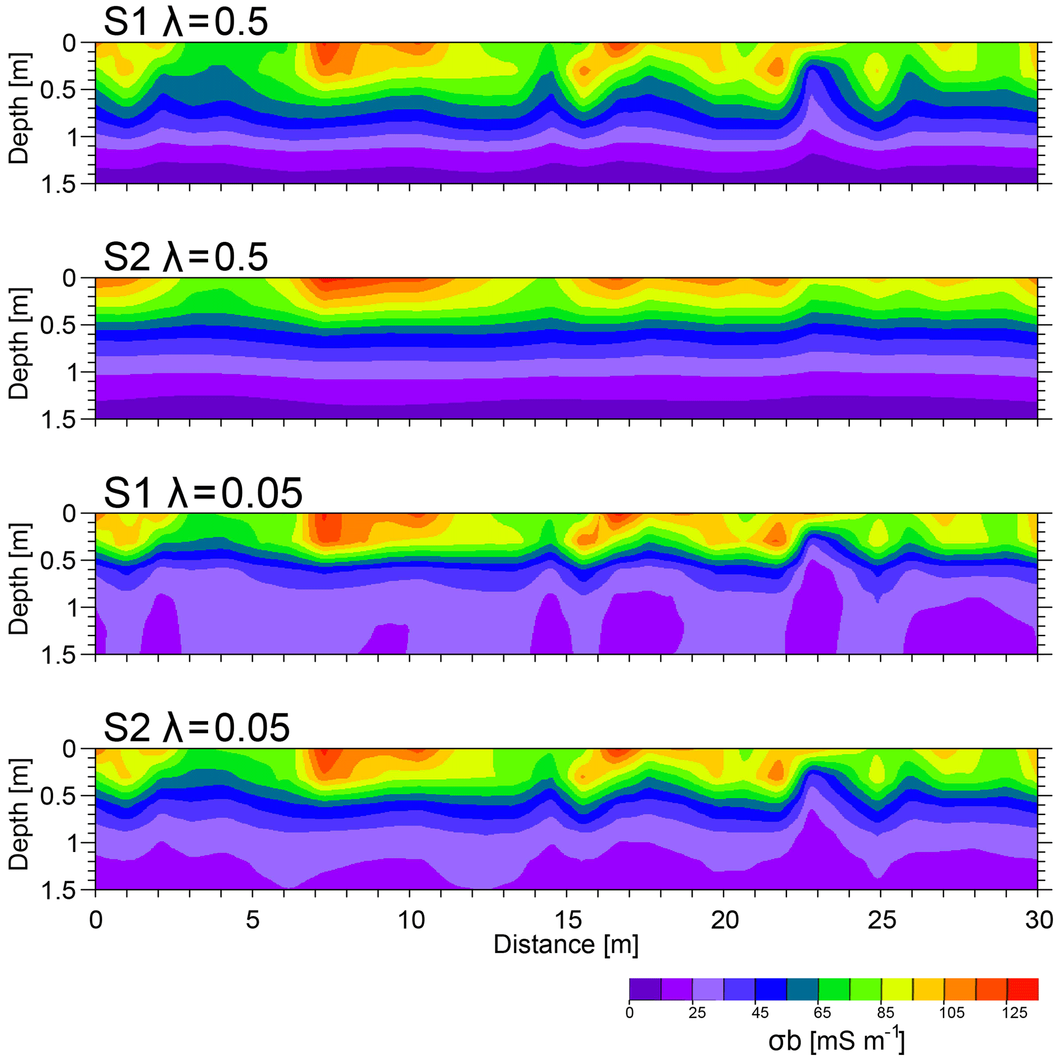
Figure 10σb distributions obtained from the inversion of the synthetic σa data (23 November), shown in Fig. 9, using four different combinations of two algorithms, S1 and S2, and λ parameters.
Ideally, the obtained σb distribution should be very similar to the one shown in Fig. 8d. However, looking closely at the obtained σb distribution, we observe that all of them are different, to some extent, to the one shown in Fig. 8d. First of all, we note that the model obtained using λ values greater than 1 (not shown here) and regardless of the choice of inversion algorithm (i.e. S1 and S2) shows a high misfit error and also significantly over-smoothed σb distribution. This is not surprising as the sharp vertical spatial variability of σb due to the saline water irrigation and soil heterogeneity as well as the shallow bedrock cannot be well resolved using high λ (over-smoothed parameters). Consequently, a high λ is not a wise choice when sharp vertical and lateral conductivity contrasts are expected in the field. The obtained model using S2 algorithm and moderate λ values (i.e. 0.5) also yields a very smooth model. In contrast, the obtained models using S1–λ=0.05, S1–λ=0.5 and S2–λ=0.05 do a better job in resolving near-surface anomalies. However, the conductivity distribution at depth is not well recovered using the S1 algorithm.
In Fig. 11, we plotted the synthetic σb distribution data against the obtained modelled σb distributions using different inversion parameters shown in Fig. 10, and we calculated the statistical scores R, RMSE and ME to further investigate the impact of the inversion algorithm and parameters in resolving the σb distributions. Firstly, we observed that both S1 and S2 algorithms underestimated the σb to some extent, judging from the ME values. The S2–λ=0.5 and S1–λ=0.05 show weaker statistical scores, with higher RMSE and ME and relatively lower R. The over-smoothed impact of S2–λ=0.5 and the resulting highest ME indicates that the S2 algorithm with moderate to high λ values is not a rational choice when large spatial and vertical variations of σb are expected. On the other hand, the lowest R and highest RMSE, obtained for S1–λ=0.05, suggest that the S1 algorithm with very small values of λ is not able to predict the spatial variation of σb well. The use of the S1 algorithm with very small values of λ usually applies an insignificant spatial constraint that may result in more inconsistency between synthetic σb and modelled σb distributions. The S2–λ=0.05 and S1–λ=0.5 show better statistical results, with higher R and lower RMSE and ME, which makes them a better choice for the inversion of field data. While both inversion parameters set present almost the same RMSE, the S2–λ=0.05 yields a higher R, suggesting that the S2–λ=0.05 can better resolve the spatial σb distributions. This is expected from a comparison of S2–λ=0.05 and S1–λ=0.5 results in Figs. 10 and 11, where a relatively lower correlation is evident between synthetic σb and modelled σb at lower ranges of σb (Fig. 11) located at depths of more than 70 cm (Figs. 10 and 11) when we used the S1– The difficulty of resolving a resistive zone at depth and beneath a conductive zone is indeed expected. In fact, the sensitivity of the EMI signals is very limited over the resistive zone, and therefore the resistive zone cannot be well resolved. The condition will be worse in our study as a resistive zone is located beneath a conductive zone: the EMI response of the subsurface will be dominated by the influence of the near-surface conductive zone. In addition, five of the six depths of investigation of the CMD Mini-Explorer are limited to the first 1 m, and, as a result, a lower resolution is expected at greater depths. The S2 algorithm did a better job in resolving the resistive zone at depth. This is because the S2 algorithm constrains the value of each cell to the reference model during the inversion process, which limits the large variations of each cell during the inversion process.
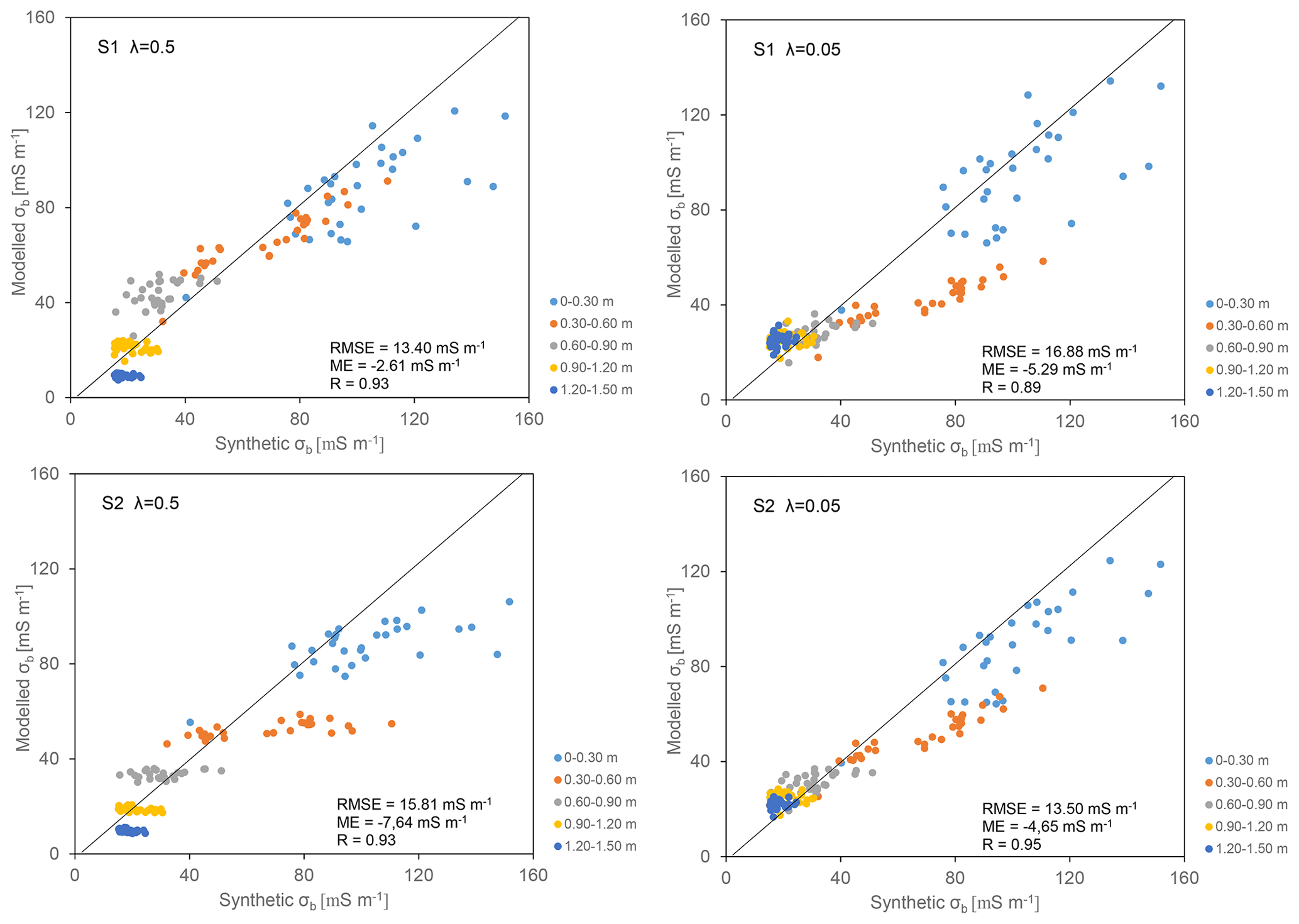
Figure 11Synthetic versus modelled σb distribution for four different combinations of S and λ inversion parameters. Different colours refer to different depths. Main statistics are also reported.
In terms of recovering the absolute values of soil electrical conductivity, it appears that all obtained models underestimate the conductivity of the anomalies near the surface. This can be explained by the over-parameterized inverse problem and the effects of smoothing from regularization applied in the inversion algorithm, as well as the impact of the resistive zone beneath the conductive zone. In addition, the six measurements per site with a site spacing of 1 m are not sufficient for recovering sharp σb variability along the transect. Measuring σa at different heights as well as smaller site spacing enables more σa data to better resolve changes which occur over short depth and length increments.
In terms of the influence of the temporal smoothing parameter (α), we explored different values (results not shown here). We noticed that the values larger than 0.1 over-smoothed the expected temporal variation, and thus the detailed variations cannot be resolved. We conclude that, for our study, a value of 0.05 is the best choice for α in resolving the temporal variation of σb.
We repeated the same analyses using 20 different synthetics transects, consisting of a random assembly of 30 interacting soil columns, each with its own hydraulic properties and depth to bedrock and different saline treatment (results not shown here). The results of our analysis show that the algorithm S2 is the best choice in the presence of a resistive zone at depth and small values of λ and α work best for dealing with the sharp lateral and temporal expected changes that occurred during the experiment. Based on the synthetic tests, the spatio-temporal algorithm S2 described in Eq. (6) with λ and α values of 0.05 and 0.05 respectively were selected to invert time lapse actual σa datasets measuring during the experiment period.
3.5 Inversion of the real time-lapse σa field data
Using the optimized inversion parameters obtained in Sect. 3.4., we inverted time-lapse σa data collected over the four experimental plots, P1, P2, P3 and P4. Figure 12 shows the σa data of the middle transect in each experimental plot (Fig. 1) for the last date of monitoring, i.e. 23 November. The σa data show a relatively similar pattern in both VCP and HCP modes, with greater σa values on ρ32 and ρ71 and the minimum σa values recorded on ρ118, indicating a conductive zone over a resistive zone. In addition, greater lateral σa changes in the VCP mode are evident along the four transects, with noticeable fluctuations in P4, suggesting greater lateral σb variations at the near surface. The σa data obtained from plot P1 and P2 show a lower range of conductivity, varying in the 20–40 mS m−1 and 20–50 mS m−1 ranges, respectively. P3 and P4 represent a higher range of conductivity, with the former in the 20–70 mS m−1 range and the latter in the 20–80 mS m−1 range.
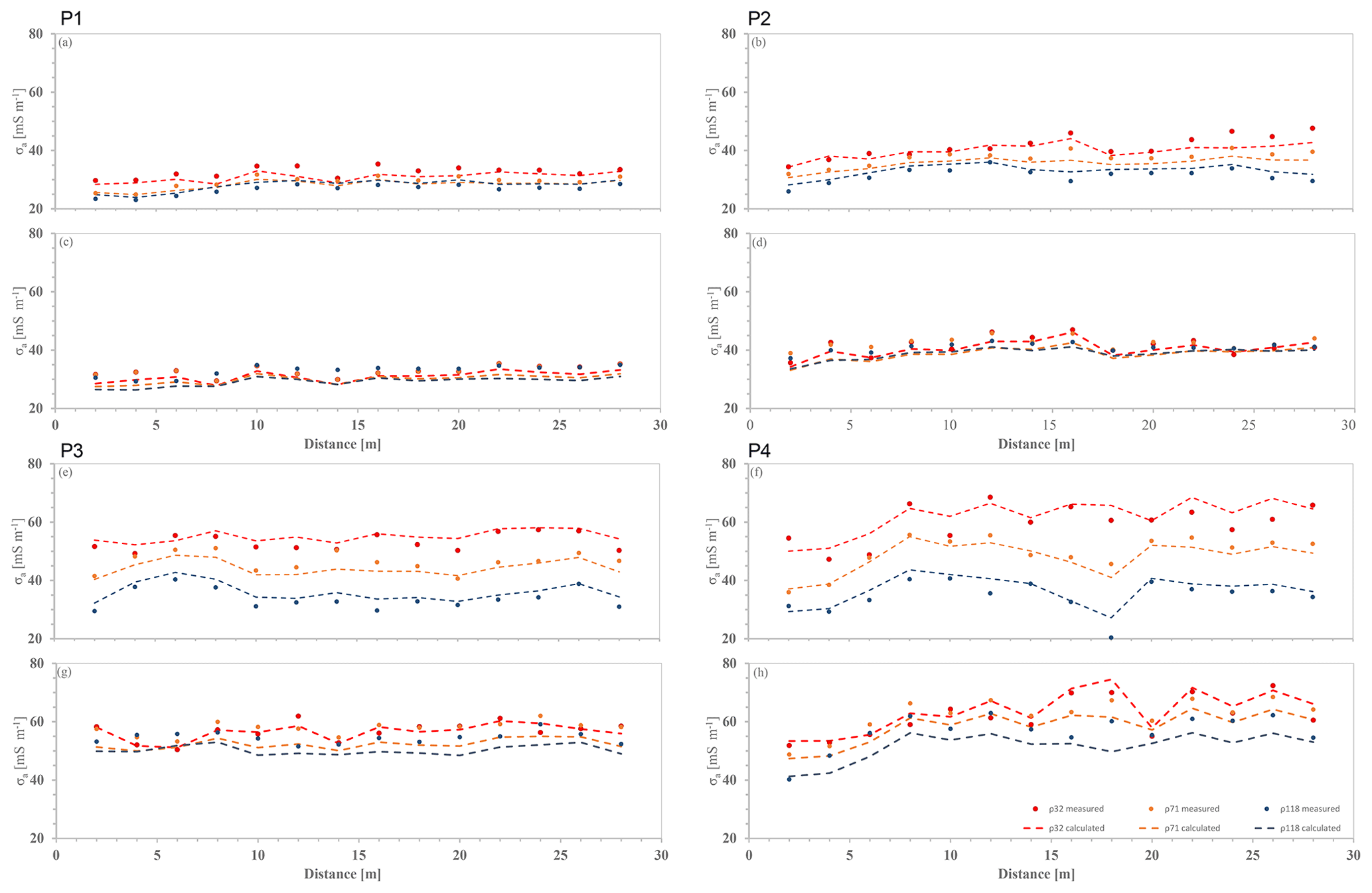
Figure 12σa distribution of the middle transect in four experimental plots, P1, P2, P3 and P4, for 23 November. Panels (a), (b), (e) and (f) show the VCP configuration, and panels (c), (d), (g) and (h) show the HCP configuration.
Figure 13 shows the time-lapse inversion results for the same transects for four dates: 17 and 26 October and 14 and 23 November 2016. The same colour scale was used for all models, allowing for a comparison of spatio-temporal variation of σb along all profiles at different times. The corresponding model responses for the last measurements on 23 November are shown in Fig. 12. The misfit errors for the P1, P2, P3 and P4 are 1.43, 1.21, 2.15 and 2.95 mS m−1, respectively, indicating a good fit between data and model responses. Slightly higher misfit errors for P3 and P4 are probably due to greater range of σa, as well as the larger lateral variations of σa. Looking at EMI models at different times and along all four experimental plots, we identify two distinct zones: a resistive zone at a depth of more than 50 cm beneath a conductive zone. The conductivity of the resistive zone varies laterally and temporally along all four transects; however, the conductivity of this zone rarely exceeds 25 mS m−1. The resistive zones in the maps shown correspond to the bedrock in the study area (Fig. 2). The conductivity of this zone is slightly lower in P3 and P4, which is probably due to the shallower bedrock in these plots. In contrast, the conductive zone at the near surface shows significant spatio-temporal conductivity changes depending on the conductivity of the injected water.
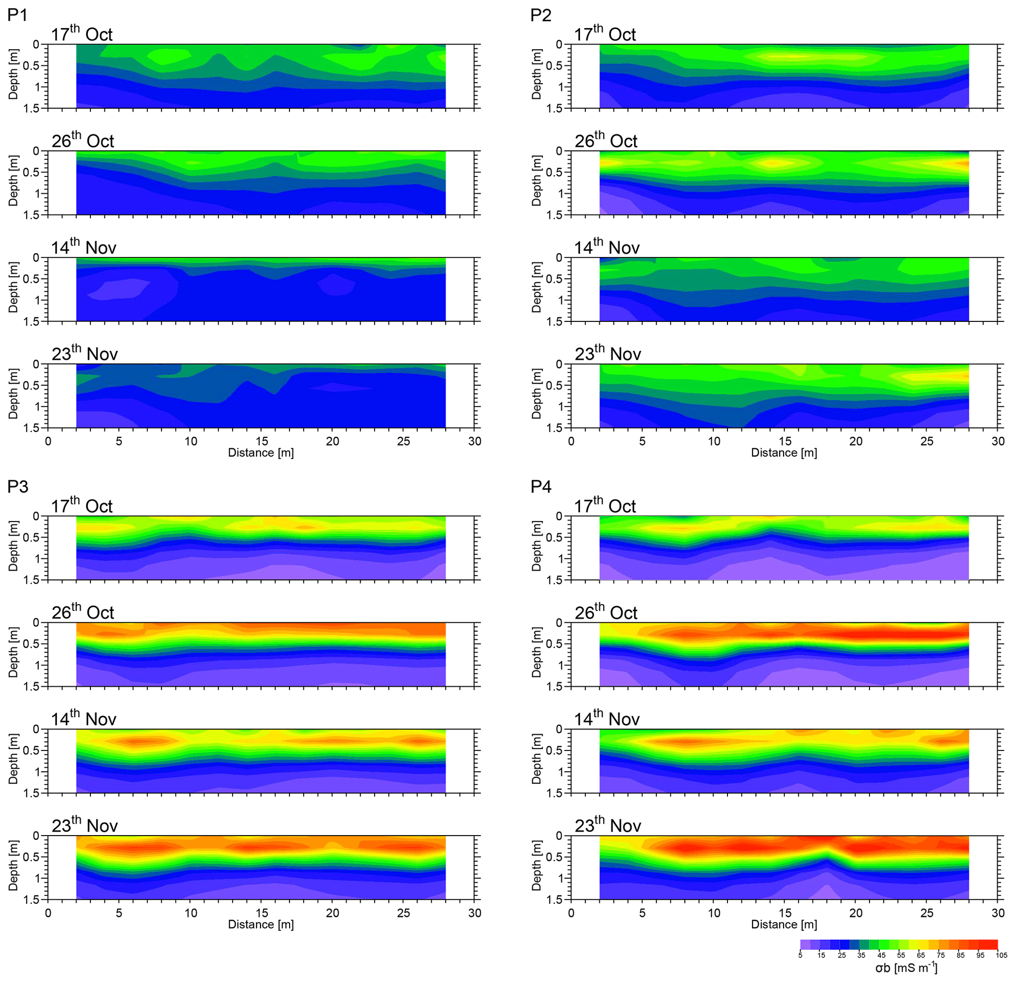
Figure 13Spatio-temporal distribution of σb along the middle transect in four experimental plots, P1, P2, P3 and P4, and for four selected dates: 17 October, 26 October, 14 November and 23 November 2016.
The time-lapse models obtained from plot P1 show the minimum spatio-temporal conductivity changes in this zone, with conductivity varying in the 30–60 mS m−1 range. The P2 plot shows larger spatial and temporal conductivity changes compared to P1, as expected, with conductivity varying between 30 and 80 mS m−1. The conductivity of this zone decreases slightly on 14 November. This is probably due to the impact of heavy rain (31 mm) on 7 November, inducing salt leaching and reducing the soil conductivity. The P3 and P4 plots show stronger conductivity changes both spatially and temporally, with conductivity varying between 50 and 100 mS m−1. The first models, obtained for 17 October, shows the minimum conductivity among the four selected dates. This is consistent with the simulated distributions shown in Fig. 8, and it is probably due to the saline front being still undispersed in the initial propagation phase (Fig. 7).
As the saline water is continuously added to the soil surface, the Cl− concentration increases in the soil and also deepens slowly in the soil profile, thus increasing soil electrical conductivity. Consequently, the higher soil conductivities seen on 23 October (Fig. 13, P3 and P4) are due to higher Cl− concentration and its propagation to deeper layers. The conductivity models obtained for 14 November show a decrease in soil conductivity in both P3 and P4, although there were six irrigations after 23 October. On the other hand, the conductive zone extends to deeper soil. This is not surprising as we already expected it from the simulations (see Fig. 8). This behaviour is probably due to the rainfall event on 7 November (as noted on P2) which diluted the Cl− concentration in the soil. This suggests that the EMI surveys and data modelling detected the expected change in Cl− concentration well.
Finally, the models obtained for the data collected on 23 November, depicted in Fig. 13, show the maximum soil conductivity and extension of the conductive zone among the selected dates in P3 and P4. A comparison of these models with our simulations results discussed in Sects. 4.1 and 4.2 shows that the increase of Cl− concentration in soil after 12 irrigation events, as well as the redistribution of Cl− during the experiment period, is the main reason for increase in soil conductivity. Judging from the water content distribution maps, obtained from numerical simulations and shown in Fig. 6, we expect very small temporal variations of water content in all experimental plots. Consequently, the temporal variations of Cl− concentration and distribution are expected to be the key factor in temporal variations of soil electrical conductivity.
From a management perspective, the discussion above suggests that using the described approach regularly after irrigation applications may allow for monitoring of salt propagation and redistribution. As water content values and patterns are expected to be quite similar at similar times after each irrigation event, changes in bulk electrical conductivities obtained by an EMI sensor will be closely related to changes in salt concentrations.
In this study, we carried out a time-lapse EMI survey over four experimental plots irrigated with water at four different salinity levels during 3 months. We examined how well the time-lapse EMI measurements and a time-lapse inversion algorithm can be used to monitor soil salinity variability in space and time through performing simulation experiments and inversion processes. Based on our detailed simulations and synthetic tests as well as the interpretation of the time-lapse models, the following main conclusions can be drawn:
-
The numerical simulations performed in this study allow for predictions of the spatial and temporal variability of soil salinity and water content during the irrigation experiment prior to the modelling of field σa data. This improves our understanding of how soil salinity and water content changes during the experiment influence σb distribution in time, which may be crucial for interpreting EMI models in terms of soil salinity and water content distribution. They also provided a synthetic time-lapse EMI dataset very similar to the field conditions, allowing for the optimization of data processing and allowing us to find the best inversion approach for the field experiment. From the synthetic analysis, we also established that the EMI measurements do not return enough subsurface information to resolve the expected sharp conductivity changes in this specific experiment.
-
A comprehensive investigation of our results and a joint interpretation of numerical simulations and time-lapse models reveal that the soil Cl− concentration change is the key factor responsible for σb changes when the EMI surveys are repeated after the irrigation at the same time. In fact, repetition of the EMI surveys after the irrigation has three main advantages: (i) the soil is wet and conductive, and, in such a condition, the signal-to-noise ratio is usually better and EMI data will be more reliable; (ii) the water content distribution will not change significantly, allowing the impact of soil salinity changes in time to be studied better; (iii) the sensitivity of σb to the Cl− concentration in wet soils is higher, and thus EMI inversion results may be used to interpret salt propagation with more confidence.
-
A previously developed least-squares 4D space–time domain inversion algorithm was implemented in this study to invert entire time-lapse EMI datasets simultaneously for monitoring soil salinity for the first time. The regularizations in this algorithm are introduced in both space and time domains to improve the stability of the inversion process and to reduce the inversion artefacts. Using a synthetic test, the applicability of the algorithm has been examined, and we showed that this approach can provide information about the conductivity variability in space and time. More synthetic tests are required to further investigate the efficiency of the inversion algorithm under different scenarios; however, we anticipate that the algorithm can be used for other EMI monitoring surveys.
-
Performing EMI surveys over four experimental plots irrigated with water at four different salinity levels, we evaluated the potential of EMI surveys for monitoring the dynamics of soil salinity due to irrigation. Comparing the EMI models obtained from four experimental sites, we showed that the σb variations are consistent with the expectations related to the amount of salt and water irrigated at each plot during the experiment. The water content did not change significantly during the EMI measurement campaigns; hence, the temporal variations of σb as well as their difference at each plot are mainly related to the soil salinity distributions. In other words, the results indicate that the applied experimental methodology is strongly capable of giving information on the spatial and temporal variability of soil salinity. Further investigations have to be conducted to use EMI sensors for monitoring salinity under significant water content changes over time. In this case, discriminating the role of water content changes and salinity changes in the σa response may be quite complicated if not impossible.
-
The EMI method provides enormous advantages over traditional methods of soil sampling because it allows for in-depth and non-invasive analysis, covering large areas in less time and at a lower cost. However, a proper interpretation of the EMI inversion models in terms of soil process is usually difficult, owing to the fact that the soil electrical conductivity is a complex function of soil properties, which may vary significantly over space and time. Thus, retrieving soil properties from EMI data requires appropriate understanding of site-specific soil processes. Our study shows that the independent interpretation of time-lapse EMI data without hydrologic insight and understanding of soil processes may be misleading. This fact highlights the necessity of collaboration of geophysicists, soil scientists and hydrologists to construct a hydrologic conceptual model which can explain the salinity and water process.
HYDRUS 1-D is public-domain software and can be downloaded from https://www.pc-progress.com/en/Default.aspx?hydrus-1d (last access: 23 March 2021) (PC-Progress, 2021). The inversion of EMI data was performed by the program developed by Fernando Montero Santos and is available on request from fasantos@fc.ul.pt.
Data of the time-lapse EMI survey over four experimental plots irrigated with water at four different salinity levels are available at https://doi.org/10.5281/zenodo.4627569 (Basile, 2021).
MF, ABa and AC conceptualized the study and developed the methodology. RDM, GD, ABa and AC set up the experiment and performed field and lab measurements. DA performed hydrological simulations. MF and FMS performed the inversion of geophysical data. MF wrote the original draft, and AC, ABa, ABi and DA contributed to the figure and table production and the reviewing and editing of the final version of the paper.
The authors declare that they have no conflict of interest.
Mohammad Farzamian was supported by a contract within project SOIL4EVER (FCT, grant no. PTDC/ASP SOL/28796/2017). We thank Maurizio Tosca (CNR) for the assistance provided during the field experiment.
This research has been supported by the project “SALTFREE – Salinization in irrigated areas: risk evaluation and prevention” under the call ARIMNet2 (Coordination of Agricultural Research in the Mediterranean; 2014–2017; https://cordis.europa.eu/project/id/618127, last access: 23 March 2021) that is an ERA-NET Action financed by the European Union under the Seventh Framework Programme for research, technological development and demonstration (grant no. 618127).
This paper was edited by Alberto Guadagnini and reviewed by two anonymous referees.
Amezketa, E.: An integrated methodology for assessing soil salinization, a pre-condition for land desertification, J. Arid Environ., 67, 594–606, https://doi.org/10.1016/j.jaridenv.2006.03.010, 2006.
Basile, A.: Dataset of EMI measurements referred to https://doi.org/10.5194/hess-25-1-2021 (Version 1.0) [Data set], Zenodo, https://doi.org/10.5281/zenodo.4627570, 2021.
Basile, A., Ciollaro, G., and Coppola, A.: Hysteresis in soil water characteristics as a key to interpreting comparisons of laboratory and field measured hydraulic properties, Water Resour. Res., 39, 1–12, https://doi.org/10.1029/2003WR002432, 2003.
Basile, A., Coppola, A., De Mascellis, R., and Randazzo, L.: Scaling Approach to Deduce Field Unsaturated Hydraulic Properties and Behavior from Laboratory Measurements on Small Cores, Vadose Zone J., 5, 1005–1016, https://doi.org/10.2136/vzj2005.0128, 2006.
Caputo, M.C., De Carlo, L., Masciopinto, C., and Nimmo, J.R.: Measurement of field-saturated hydraulic conductivity on fractured rock outcrops near Altamura (Southern Italy) with an adjustable large ring infiltrometer, Environ. Earth Sci., 60, 583–590, https://doi.org/10.1007/s12665-009-0198-y, 2010.
Caputo M.C., Maggi S., and Turturro A.C.: Calculation of Water Retention Curves of Rock Samples by Differential Evolution, in: Engineering Geology for Society and Territory, edited by Lollino G., Manconi A., Guzzetti F., Culshaw M., Bobrowsky P., Luino F. (eds), Volume 5, Springer, Cham, https://doi.org/10.1007/978-3-319-09048-1, 2015.
Carsel, R. F. and Parrish, R. S.: Developing joint probability distributions of soil water retention characteristics, Water Resour. Res., 24, 755–769, https://doi.org/10.1029/WR024i005p00755, 1988.
Cook, P. G. and Walker, G. R.: Depth Profiles of Electrical Conductivity from Linear Combinations of Electromagnetic Induction Measurements, Soil Sci. Soc. Am. J., 56, 1015–1022, https://doi.org/10.2136/sssaj1992.03615995005600040003x, 1992.
Coppola, A., Chaali, N., Dragonetti, G., Lamaddalena, N., and Comegna, A.: Root uptake under non-uniform root-zone salinity, Ecohydrology, 8, 1363–1379, https://doi.org/10.1002/eco.1594, 2015.
Coppola, A., Comegna, A., Dragonetti, G., Lamaddalena, N., Kader, A. M., and Comegna, V.: Average moisture saturation effects on temporal stability of soil water spatial distribution at field scale, Soil Till. Res., 114, 155–164, https://doi.org/10.1016/j.still.2011.04.009, 2011a.
Coppola, A., Comegna, A., Dragonetti, G., Dyck, M., Basile, A., Lamaddalena, N., Kassab, M., and Comegna, V.: Solute transport scales in an unsaturated stony soil, Adv. Water Resour., 34, 747–759, https://doi.org/10.1016/j.advwatres.2011.03.006, 2011b.
Coppola, A., Dragonetti, G., Comegna, A., Lamaddalena, N., Caushi, B., Haikal, M. A., and Basile, A.: Measuring and modeling water content in stony soils, Soil Till. Res., 128, 9–22, https://doi.org/10.1016/j.still.2012.10.006, 2013.
Coppola, A., Smettem, K., Ajeel, A., Saeed, A., Dragonetti, G., Comegna, A., Lamaddalena, N., and Vacca, A.: Calibration of an electromagnetic induction sensor with time-domain reflectometry data to monitor rootzone electrical conductivity under saline water irrigation, Eur. J. Soil Sci., 67, 737–748, https://doi.org/10.1111/ejss.12390, 2016.
Corwin, D. L. and Lesch, S. M.: Apparent soil electrical conductivity measurements in agriculture, Comput. Electron. Agr., 46, 11–43, https://doi.org/10.1016/j.compag.2004.10.005, 2005.
Corwin, D. L. and Rhoades, J. D.: Measurement of Inverted Electrical Conductivity Profiles Using Electromagnetic Induction, Soil Sci. Soc. Am. J., 48, 288–291, https://doi.org/10.2136/sssaj1984.03615995004800020011x, 1984.
Corwin, D. L., Lesch, S. M., Oster, J. D., and Kaffka, S. R.: Monitoring management-induced spatio–temporal changes in soil quality through soil sampling directed by apparent electrical conductivity, Geoderma, 131, 369–387, https://doi.org/10.1016/j.geoderma.2005.03.014, 2006.
Daily, W., Ramirez, A., LaBrecque, D., and Nitao, J.: Electrical resistivity tomography of vadose water movement, Water Resour. Res., 28, 1429–1442, https://doi.org/10.1029/91WR03087, 1992.
Dane, J. and Hopmans, J.: Water retention and storage, in: Methods of Soil Analysis, Part 4, Physical Methods, SSSA, Book Series 5, 671–720, Madison, Wisconsin, 2003.
Dragonetti, G., Comegna, A., Ajeel, A., Deidda, G. P., Lamaddalena, N., Rodriguez, G., Vignoli, G., and Coppola, A.: Calibrating electromagnetic induction conductivities with time-domain reflectometry measurements, Hydrol. Earth Syst. Sci., 22, 1509–1523, https://doi.org/10.5194/hess-22-1509-2018, 2018.
Farzamian, M., Monteiro Santos, F. A., and Khalil, M. A.: Application of EM38 and ERT methods in estimation of saturated hydraulic conductivity in unsaturated soil, J. Appl. Geophys., 112, 175–189, https://doi.org/10.1016/j.jappgeo.2014.11.016, 2015a.
Farzamian, M., Monteiro Santos, F. A., and Khalil, M. A.: Estimation of unsaturated hydraulic parameters in sandstone using electrical resistivity tomography under a water injection test, J. Appl. Geophys., 121, 71–83, https://doi.org/10.1016/j.jappgeo.2015.07.014, 2015b.
Farzamian, M., Paz, M. C., Paz, A. M., Castanheira, N. L., Gonçalves, M. C., Monteiro Santos, F. A., and Triantafilis, J.: Mapping soil salinity using electromagnetic conductivity imaging–A comparison of regional and location-specific calibrations, Land. Degrad. Dev., 30, 1393–1406, https://doi.org/10.1002/ldr.3317, 2019.
Ganjegunte, G. K., Sheng, Z., and Clark, J. A.: Soil salinity and sodicity appraisal by electromagnetic induction in soils irrigated to grow cotton, Land. Degrad. Dev., 25, 228–235, https://doi.org/10.1002/ldr.1162, 2014.
Geeson, N. A., Brandt, C. J., and Thornes, J. B.: Mediterranean desertification: a mosaic of processes and responses, Wiley Interscience, Cambridge, 2002.
Goff, A., Huang, J., Wong, V. N. L., Monteiro Santos, F. A., Wege, R., and Triantafilis, J.: Electromagnetic Conductivity Imaging of Soil Salinity in an Estuarine-Alluvial Landscape, Soil Sci. Soc. Am. J., 78, 1686–1693, https://doi.org/10.2136/sssaj2014.02.0078, 2014.
Gonçalves, R., Farzamian, M., Monteiro Santos, F. A., Represas, P., Mota Gomes, A., Lobo de Pina, A. F., and Almeida, E. P.: Application of Time-Domain Electromagnetic Method in Investigating Saltwater Intrusion of Santiago Island (Cape Verde), Pure Appl. Geophys., 174, 4171–4182, https://doi.org/10.1007/s00024-017-1656-1, 2017.
Hayley, K., Pidlisecky, A., and Bentley, L. R.: Simultaneous time-lapse electrical resistivity inversion, J. Appl. Geophys., 75, 401–411, https://doi.org/10.1016/j.jappgeo.2011.06.035, 2011.
Huang, J., Koganti, T., Santos, F. A. M., and Triantafilis, J.: Mapping soil salinity and a fresh-water intrusion in three-dimensions using a quasi-3d joint-inversion of DUALEM-421S and EM34 data, Sci. Total Environ., 577, 395–404, https://doi.org/10.1016/j.scitotenv.2016.10.224, 2017.
Huang, J., Monteiro Santos, F. A., and Triantafilis, J.: Mapping soil water dynamics and a moving wetting front by spatiotemporal inversion of electromagnetic induction data, Water Resour. Res., 52, 9131–9145, https://doi.org/10.1002/2016WR019330, 2016.
Jadoon, K. Z., Altaf, M. U., McCabe, M. F., Hoteit, I., Muhammad, N., Moghadas, D., and Weihermüller, L.: Inferring soil salinity in a drip irrigation system from multi-configuration EMI measurements using adaptive Markov chain Monte Carlo, Hydrol. Earth Syst. Sci., 21, 5375–5383, https://doi.org/10.5194/hess-21-5375-2017, 2017.
Kim, J. H., Yi, M. J., Park, S. G., and Kim, J. G.: 4D inversion of DC resistivity monitoring data acquired over a dynamically changing earth model, J. Appl. Geophys., 68, 522–532, https://doi.org/10.1016/j.jappgeo.2009.03.002, 2009.
Kutilek, M. and D. R. Nielsen, Soil Hydrology, Catena, Cremlingen-Destedt, Germany, 370 pp., ISBN 978-3-510-65387-4, 1994.
LaBrecque, D. J. and Yang, X.: Difference Inversion of ERT Data: a Fast Inversion Method for 3D In Situ Monitoring, J. Environ. Eng. Geoph., 6, 83–89, https://doi.org/10.4133/JEEG6.2.83, 2001.
Lesch, S. M., Strauss, D. J., and Rhoades, J. D.: Spatial Prediction of Soil Salinity Using Electromagnetic Induction Techniques: 1. Statistical Prediction Models: A Comparison of Multiple Linear Regression and Cokriging, Water Resour. Res., 31, 373–386, https://doi.org/10.1029/94WR02179, 1995.
Malicki, M. A. and Walczak, R. T.: Evaluating soil salinity status from bulk electrical conductivity and permittivity, Eur. J. Soil Sci., 50, 505–514, https://doi.org/10.1046/j.1365-2389.1999.00245.x, 1999.
Mallants, D., Jacques, D., Vanclooster, M., Diels, J., and Feyen, J.: A stochastic approach to simulate water flow in a macroporous soil, Geoderma, 70, 299–324, 1996.
Mallants, D., Van Genuchten, M. T., Šimůnek, J., Jacques, D., and Seetharam, S.: Leaching of Contaminants to Groundwater, in: Dealing with Contaminated Sites, edited by: Swartjes, F., Springer, Dordrecht, https://doi.org/10.1007/978-90-481-9757-6_18, 2011.
Maréchal, B., Prosperi, P., and Rusco, E.: Implications of soil threats on agricultural areas in Europe, in: Threats to Soil Quality in Europe, edited by: Toth, G., Montanarella, L., and Rusco, E., Office for Official Publications of the European Communities, Luxembourg, 129–138, https://doi.org/10.2788/8647, 2008.
Moghadas, D.: Probabilistic Inversion of Multiconfiguration Electromagnetic Induction Data Using Dimensionality Reduction Technique: A Numerical Study, Vadose Zone J., 18, 1–16, https://doi.org/10.2136/vzj2018.09.0183, 2019.
Monteiro Santos, F. A.: 1D laterally constrained inversion of EM34 profiling data, J. Appl. Geophys., 56, 123–134, https://doi.org/10.1016/j.jappgeo.2004.04.005, 2004.
Paz, A. M., Castanheira, N., Farzamian, M., Paz, M. C., Gonçalves, M. C., Monteiro Santos, F. A., and Triantafilis, J.: Prediction of soil salinity and sodicity using electromagnetic conductivity imaging, Geoderma, 361, 114086, https://doi.org/10.1016/j.geoderma.2019.114086, 2020a.
Paz, M. C., Farzamian, M., Paz, A. M., Castanheira, N. L., Gonçalves, M. C., and Monteiro Santos, F.: Assessing soil salinity using time-lapse electromagnetic conductivity imaging, SOIL, 6, 499–511, https://doi.org/10.5194/soil-6-499-2020, 2020b.
Paz, M. C., Farzamian, M., Santos, F. M., Gonçalves, M. C., Paz, A. M., Castanheira, N. L., and Triantafilis, J.: Potential to map soil salinity using inversion modelling of EM38 sensor data, First Break, 37, 35–39, https://doi.org/10.3997/1365-2397.2019019, 2019.
PC-Progress: Hydrus-1D for Windows, Version 4.xx, available at: https://www.pc-progress.com/en/Default.aspx?hydrus-1d, last access: 23 March 2021.
Reynolds, W. D. and Elrick, D.: Constant head soil core (tank) method, in: Methods of Soil Analysis, Part 4, Physical Methods, SSSA Book series 5, 5, 809–812, Madison, WI, USA, 2003.
Schamper, C., Rejiba, F., and Guérin, R.: 1D single-site and laterally constrained inversion of multifrequency and multicomponent ground-based electromagnetic induction data – Application to the investigation of a near-surface clayey overburden, Geophysics, 77, WB19–WB35, https://doi.org/10.1190/geo2011-0358.1, 2012.
Shanahan, P. W., Binley, A., Whalley, W. R., and Watts, C. W.: The Use of Electromagnetic Induction to Monitor Changes in Soil Moisture Profiles Beneath Different Wheat Genotypes, Soil Sci. Soc. Am. J., 79, 459–466, https://doi.org/10.2136/sssaj2014.09.0360, 2015.
Shrivastava, P. and Kumar, R.: Soil salinity: A serious environmental issue and plant growth promoting bacteria as one of the tools for its alleviation, Saudi J. Biol. Sci., 22, 123–131 https://doi.org/10.1016/j.sjbs.2014.12.001, 2015.
Šimůnek, J., van Genuchten, M. T., and Šejna, M.: Recent Developments and Applications of the HYDRUS Computer Software Packages, Vadose Zone J., 15, 1–15, https://doi.org/10.2136/vzj2016.04.0033, 2016.
Slavich, P. and Petterson, G.: Estimating average rootzone salinity from electromagnetic induction (EM-38) measurements, Soil Res., 28, 453, https://doi.org/10.1071/SR9900453, 1990.
Tarantola, A.: Inverse problem theory, 1st Edn., Elsevier, Amsterdam, ISBN 9780444599674, 1987.
Triantafilis, J., Laslett, G. M., and McBratney, A. B.: Calibrating an Electromagnetic Induction Instrument to Measure Salinity in Soil under Irrigated Cotton, Soil Sci. Soc. Am. J., 64, 1009–1017, https://doi.org/10.2136/sssaj2000.6431009x, 2000.
van Genuchten, M. T.: A closed-form equation for predicting the hydraulic conductivity of unsaturated soils, Soil Sci. Soc. Am. J., 44, 892–898, 1980.
von Hebel, C., Rudolph, S., Mester, A., Huisman, J. A., Kumbhar, P., Vereecken, H., and van der Kruk, J.: Three-dimensional imaging of subsurface structural patterns using quantitative large-scale multiconfiguration electromagnetic induction data, Water Resour. Res., 50, 2732–2748, https://doi.org/10.1002/2013WR014864, 2014.
Whalley, W. R., Binley, A. M., Watts, C. W., Shanahan, P., Dodd, I. C., Ober, E. S., Ashton, R. W., Webster, C. P., White, R. P., and Hawkesford, M. J.: Methods to estimate changes in soil water for phenotyping root activity in the field, Plant Soil, 415, 407–422. https://doi.org/10.1007/s11104-016-3161-1, 2017.
Yao, R. and Yang, J.: Quantitative evaluation of soil salinity and its spatial distribution using electromagnetic induction method, Agr. Water Manage., 97, 1961–1970, https://doi.org/10.1016/j.agwat.2010.02.001, 2010.
Zare, E., Li, N., Khongnawang, T., Farzamian, M., and Triantafilis, J.: Identifying Potential Leakage Zones in an Irrigation Supply Channel by Mapping Soil Properties Using Electromagnetic Induction, Inversion Modelling and a Support Vector Machine, Soil Syst., 4, 25, https://doi.org/10.3390/soilsystems4020025, 2020.
Zhang, Z., Routh, P. S., Oldenburg, D. W., Alumbaugh, D. L., and Newman, G. A.: Reconstruction of 1D conductivity from dual-loop EM data, Geophysics, 65, 492–501, https://doi.org/10.1190/1.1444743, 2000.